practical numerical methods in physics and astronomy ...patscott/teaching/numeric/lec 3.pdf · the...
TRANSCRIPT
The problemSolutions
Practical Numerical Methods in Physics andAstronomy
Lecture 3 – Root Finding
Pat Scott
Department of Physics, McGill University
January 23, 2013
Slides available fromhttp://www.physics.mcgill.ca/̃ patscott
PHYS 606 Practical Numerical Methods, Winter 2013 Lecture 3 – Root Finding
The problemSolutions
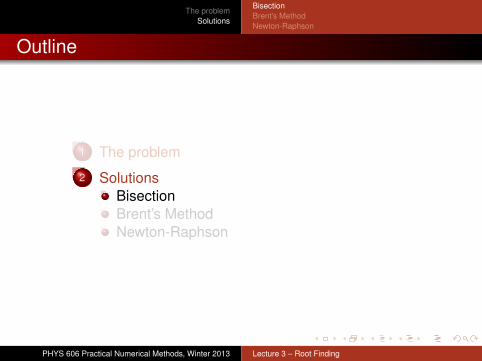
Outline
1 The problem
2 SolutionsBisectionBrent’s MethodNewton-Raphson
PHYS 606 Practical Numerical Methods, Winter 2013 Lecture 3 – Root Finding
The problemSolutions
Outline
1 The problem
2 SolutionsBisectionBrent’s MethodNewton-Raphson
PHYS 606 Practical Numerical Methods, Winter 2013 Lecture 3 – Root Finding
The problemSolutions
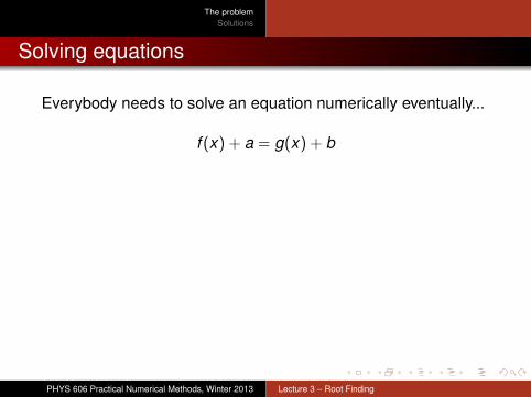
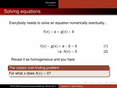
Solving equations
Everybody needs to solve an equation numerically eventually...
f (x) + a = g(x) + b
f (x)− g(x) + a− b = 0 (1)i.e. h(x) = 0 (2)
Recast it as homogeneous and you have
The classic root-finding problem
For what x does h(x) = 0?
PHYS 606 Practical Numerical Methods, Winter 2013 Lecture 3 – Root Finding
The problemSolutions
Solving equations
Everybody needs to solve an equation numerically eventually...
f (x) + a = g(x) + b
f (x)− g(x) + a− b = 0 (1)i.e. h(x) = 0 (2)
Recast it as homogeneous and you have
The classic root-finding problem
For what x does h(x) = 0?
PHYS 606 Practical Numerical Methods, Winter 2013 Lecture 3 – Root Finding

The problemSolutions
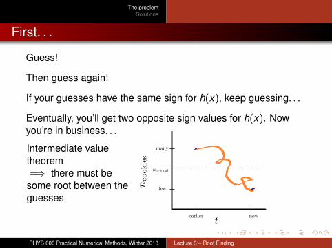
First. . .
Guess!
Then guess again!
If your guesses have the same sign for h(x), keep guessing. . .
Eventually, you’ll get two opposite sign values for h(x). Nowyou’re in business. . .
Intermediate valuetheorem=⇒ there must besome root between theguesses
PHYS 606 Practical Numerical Methods, Winter 2013 Lecture 3 – Root Finding

The problemSolutions
First. . .
Guess!
Then guess again!
If your guesses have the same sign for h(x), keep guessing. . .
Eventually, you’ll get two opposite sign values for h(x). Nowyou’re in business. . .
Intermediate valuetheorem=⇒ there must besome root between theguesses
PHYS 606 Practical Numerical Methods, Winter 2013 Lecture 3 – Root Finding
The problemSolutions
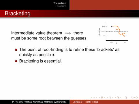
Bracketing
Intermediate value theorem =⇒ theremust be some root between the guesses
The point of root-finding is to refine these ‘brackets’ asquickly as possible.Bracketing is essential.
If all your guesses have the same sign for h(x), you’re a bitscrewed – find something better than guessing. Actually,work out how to guess smarter.Always eyeball your function before trying to find its roots,unless you know it very well.
PHYS 606 Practical Numerical Methods, Winter 2013 Lecture 3 – Root Finding
The problemSolutions
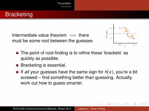
Bracketing
Intermediate value theorem =⇒ theremust be some root between the guesses
The point of root-finding is to refine these ‘brackets’ asquickly as possible.Bracketing is essential.If all your guesses have the same sign for h(x), you’re a bitscrewed – find something better than guessing. Actually,work out how to guess smarter.
Always eyeball your function before trying to find its roots,unless you know it very well.
PHYS 606 Practical Numerical Methods, Winter 2013 Lecture 3 – Root Finding
The problemSolutions
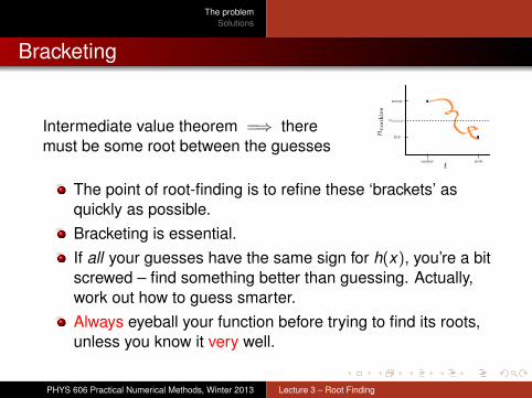
Bracketing
Intermediate value theorem =⇒ theremust be some root between the guesses
The point of root-finding is to refine these ‘brackets’ asquickly as possible.Bracketing is essential.If all your guesses have the same sign for h(x), you’re a bitscrewed – find something better than guessing. Actually,work out how to guess smarter.Always eyeball your function before trying to find its roots,unless you know it very well.
PHYS 606 Practical Numerical Methods, Winter 2013 Lecture 3 – Root Finding
The problemSolutions
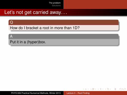
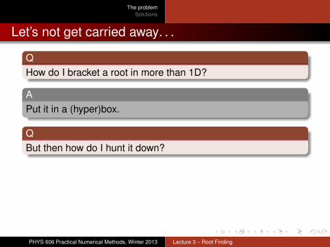
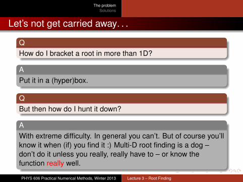
Let’s not get carried away. . .
QHow do I bracket a root in more than 1D?
APut it in a (hyper)box.
QBut then how do I hunt it down?
AWith extreme difficulty. In general you can’t. But of course you’llknow it when (if) you find it :) Multi-D root finding is a dog –don’t do it unless you really, really have to – or know thefunction really well.
PHYS 606 Practical Numerical Methods, Winter 2013 Lecture 3 – Root Finding
The problemSolutions
Let’s not get carried away. . .
QHow do I bracket a root in more than 1D?
APut it in a (hyper)box.
QBut then how do I hunt it down?
AWith extreme difficulty. In general you can’t. But of course you’llknow it when (if) you find it :) Multi-D root finding is a dog –don’t do it unless you really, really have to – or know thefunction really well.
PHYS 606 Practical Numerical Methods, Winter 2013 Lecture 3 – Root Finding

The problemSolutions
Let’s not get carried away. . .
QHow do I bracket a root in more than 1D?
APut it in a (hyper)box.
QBut then how do I hunt it down?
QWhy the hell does Pat only ask questions that have no realanswers?
PHYS 606 Practical Numerical Methods, Winter 2013 Lecture 3 – Root Finding
The problemSolutions
BisectionBrent’s MethodNewton-Raphson
Outline
1 The problem
2 SolutionsBisectionBrent’s MethodNewton-Raphson
PHYS 606 Practical Numerical Methods, Winter 2013 Lecture 3 – Root Finding
The problemSolutions
BisectionBrent’s MethodNewton-Raphson
Outline
1 The problem
2 SolutionsBisectionBrent’s MethodNewton-Raphson
PHYS 606 Practical Numerical Methods, Winter 2013 Lecture 3 – Root Finding

The problemSolutions
BisectionBrent’s MethodNewton-Raphson
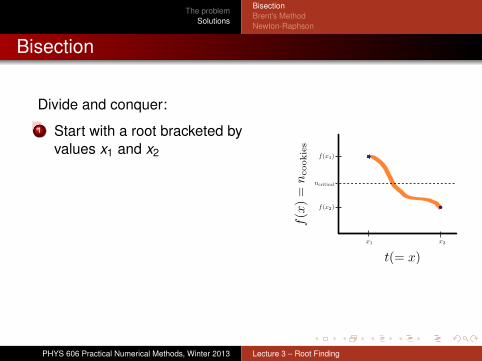
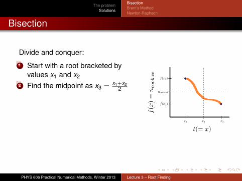
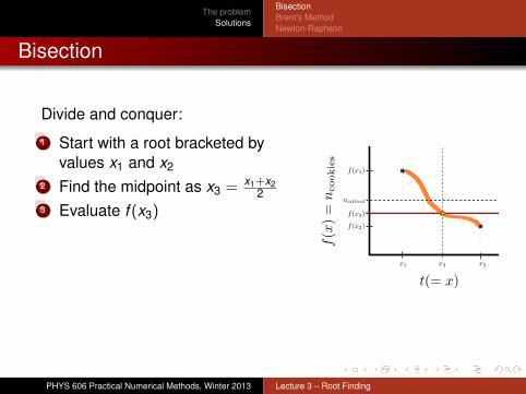
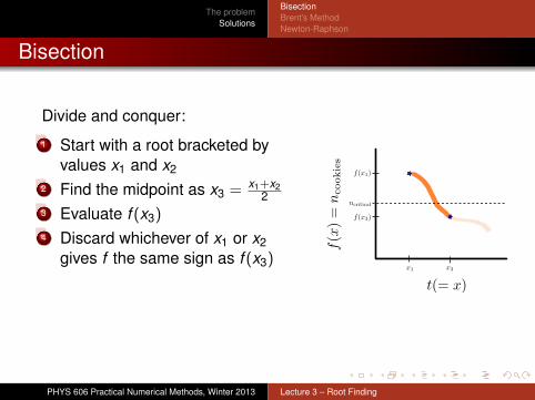
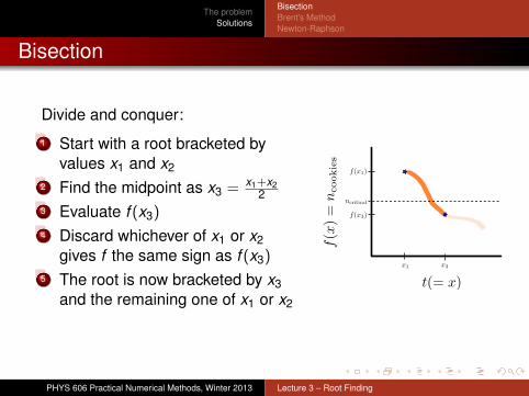
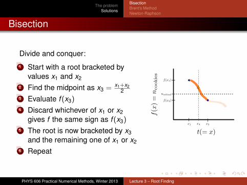
Bisection
Divide and conquer:
1 Start with a root bracketed byvalues x1 and x2
2 Find the midpoint as x3 = x1+x22
3 Evaluate f (x3)
4 Discard whichever of x1 or x2gives f the same sign as f (x3)
5 The root is now bracketed by x3and the remaining one of x1 or x2
6 Repeat
PHYS 606 Practical Numerical Methods, Winter 2013 Lecture 3 – Root Finding
The problemSolutions
BisectionBrent’s MethodNewton-Raphson
Bisection
Divide and conquer:
1 Start with a root bracketed byvalues x1 and x2
2 Find the midpoint as x3 = x1+x22
3 Evaluate f (x3)
4 Discard whichever of x1 or x2gives f the same sign as f (x3)
5 The root is now bracketed by x3and the remaining one of x1 or x2
6 Repeat
PHYS 606 Practical Numerical Methods, Winter 2013 Lecture 3 – Root Finding
The problemSolutions
BisectionBrent’s MethodNewton-Raphson
Improving on bisection
General idea for improving is to use some (convergent)approximation / guess function
Linear interpolation = secant, false position methodExponential functions = Ridder’s methodQuadratic interpolation (+bisection) = Müller’s methodInverse quadratic interpol (+bisection) = Brent’s methodTangent extrapolation = Newton-Raphson
PHYS 606 Practical Numerical Methods, Winter 2013 Lecture 3 – Root Finding
The problemSolutions
BisectionBrent’s MethodNewton-Raphson
Outline
1 The problem
2 SolutionsBisectionBrent’s MethodNewton-Raphson
PHYS 606 Practical Numerical Methods, Winter 2013 Lecture 3 – Root Finding
The problemSolutions
BisectionBrent’s MethodNewton-Raphson
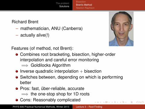
Richard Brent– mathematician, ANU (Canberra)– actually alive(!)
Features (of method, not Brent):Combines root bracketing, bisection, higher-orderinterpolation and careful error monitoring=⇒ Goldilocks AlgorithmInverse quadratic interpolation + bisectionSwitches between, depending on which is performingbetterPros: fast, über-reliable, accurate=⇒ the one-stop shop for 1D rootsCons: Reasonably complicated
PHYS 606 Practical Numerical Methods, Winter 2013 Lecture 3 – Root Finding
The problemSolutions
BisectionBrent’s MethodNewton-Raphson
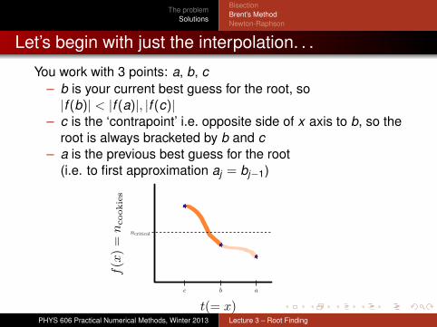
Let’s begin with just the interpolation. . .
You work with 3 points: a, b, c– b is your current best guess for the root, so|f (b)| < |f (a)|, |f (c)|
– c is the ‘contrapoint’ i.e. opposite side of x axis to b, so theroot is always bracketed by b and c
– a is the previous best guess for the root(i.e. to first approximation aj = bj−1)
PHYS 606 Practical Numerical Methods, Winter 2013 Lecture 3 – Root Finding
The problemSolutions
BisectionBrent’s MethodNewton-Raphson
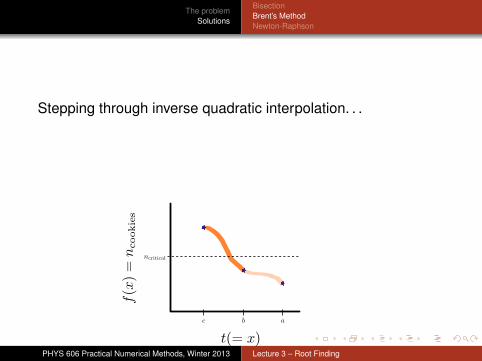
Stepping through inverse quadratic interpolation. . .
QHow do we proceed when we are down to only 2 points(e.g. here, and at the start of the search)?
AQuestion 2.a) in Assignment 2 deals with this.
PHYS 606 Practical Numerical Methods, Winter 2013 Lecture 3 – Root Finding
QHow do we proceed when we are down to only 2 points(e.g. here, and at the start of the search)?
AQuestion 2.a) in Assignment 2 deals with this.
The problemSolutions
BisectionBrent’s MethodNewton-Raphson
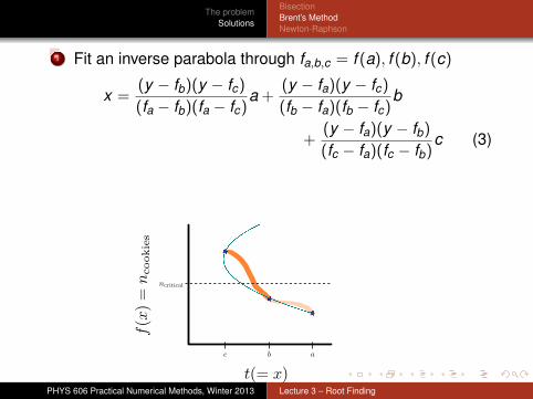
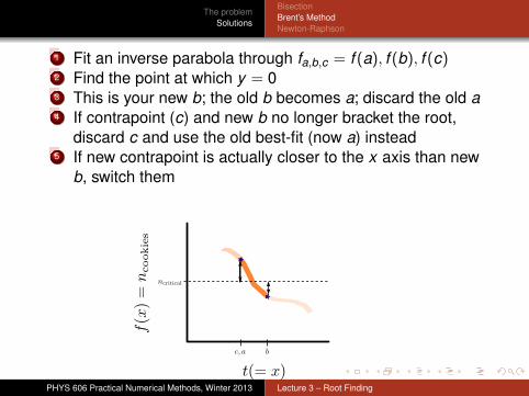
1 Fit an inverse parabola through fa,b,c = f (a), f (b), f (c)
x =(y − fb)(y − fc)(fa − fb)(fa − fc)
a +(y − fa)(y − fc)(fb − fa)(fb − fc)
b
+(y − fa)(y − fb)
(fc − fa)(fc − fb)c (3)
2 Find the point at which y = 03 This is your new b; the old b becomes a; discard the old a4 If contrapoint (c) and new b no longer bracket the root,
discard c and use the old best-fit (now a) instead5 If new contrapoint is actually closer to the x axis than new
b, switch them
QHow do we proceed when we are down to only 2 points(e.g. here, and at the start of the search)?
AQuestion 2.a) in Assignment 2 deals with this.
PHYS 606 Practical Numerical Methods, Winter 2013 Lecture 3 – Root Finding
QHow do we proceed when we are down to only 2 points(e.g. here, and at the start of the search)?
AQuestion 2.a) in Assignment 2 deals with this.
The problemSolutions
BisectionBrent’s MethodNewton-Raphson
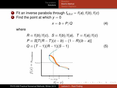
1 Fit an inverse parabola through fa,b,c = f (a), f (b), f (c)2 Find the point at which y = 0
x = b + P/Q (4)
where
R ≡ f (b)/f (c), S ≡ f (b)/f (a), T ≡ f (a)/f (c)
P ≡ S[T (R − T )(c − b)− (1− R)(b − a)]
Q ≡ (T − 1)(R − 1)(S − 1) (5)
3 This is your new b; the old b becomes a; discard the old a4 If contrapoint (c) and new b no longer bracket the root,
discard c and use the old best-fit (now a) instead5 If new contrapoint is actually closer to the x axis than new
b, switch them
QHow do we proceed when we are down to only 2 points(e.g. here, and at the start of the search)?
AQuestion 2.a) in Assignment 2 deals with this.
PHYS 606 Practical Numerical Methods, Winter 2013 Lecture 3 – Root Finding
QHow do we proceed when we are down to only 2 points(e.g. here, and at the start of the search)?
AQuestion 2.a) in Assignment 2 deals with this.
The problemSolutions
BisectionBrent’s MethodNewton-Raphson
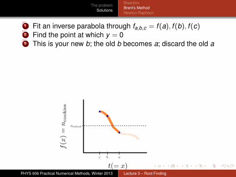
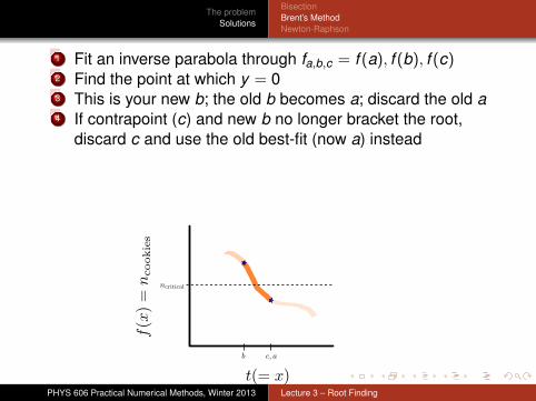
1 Fit an inverse parabola through fa,b,c = f (a), f (b), f (c)2 Find the point at which y = 03 This is your new b; the old b becomes a; discard the old a
4 If contrapoint (c) and new b no longer bracket the root,discard c and use the old best-fit (now a) instead
5 If new contrapoint is actually closer to the x axis than newb, switch them
QHow do we proceed when we are down to only 2 points(e.g. here, and at the start of the search)?
AQuestion 2.a) in Assignment 2 deals with this.
PHYS 606 Practical Numerical Methods, Winter 2013 Lecture 3 – Root Finding
QHow do we proceed when we are down to only 2 points(e.g. here, and at the start of the search)?
AQuestion 2.a) in Assignment 2 deals with this.
The problemSolutions
BisectionBrent’s MethodNewton-Raphson
1 Fit an inverse parabola through fa,b,c = f (a), f (b), f (c)2 Find the point at which y = 03 This is your new b; the old b becomes a; discard the old a4 If contrapoint (c) and new b no longer bracket the root,
discard c and use the old best-fit (now a) instead
5 If new contrapoint is actually closer to the x axis than newb, switch them
QHow do we proceed when we are down to only 2 points(e.g. here, and at the start of the search)?
AQuestion 2.a) in Assignment 2 deals with this.
PHYS 606 Practical Numerical Methods, Winter 2013 Lecture 3 – Root Finding
QHow do we proceed when we are down to only 2 points(e.g. here, and at the start of the search)?
AQuestion 2.a) in Assignment 2 deals with this.
The problemSolutions
BisectionBrent’s MethodNewton-Raphson
1 Fit an inverse parabola through fa,b,c = f (a), f (b), f (c)2 Find the point at which y = 03 This is your new b; the old b becomes a; discard the old a4 If contrapoint (c) and new b no longer bracket the root,
discard c and use the old best-fit (now a) instead5 If new contrapoint is actually closer to the x axis than new
b, switch them
QHow do we proceed when we are down to only 2 points(e.g. here, and at the start of the search)?
AQuestion 2.a) in Assignment 2 deals with this.
PHYS 606 Practical Numerical Methods, Winter 2013 Lecture 3 – Root Finding
QHow do we proceed when we are down to only 2 points(e.g. here, and at the start of the search)?
AQuestion 2.a) in Assignment 2 deals with this.
The problemSolutions
BisectionBrent’s MethodNewton-Raphson
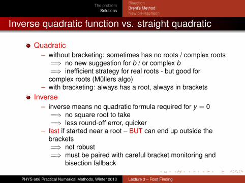
Inverse quadratic function vs. straight quadratic
Quadratic– without bracketing: sometimes has no roots / complex roots
=⇒ no new suggestion for b / or complex b=⇒ inefficient strategy for real roots - but good forcomplex roots (Müllers algo)
– with bracketing: always has a root, always in bracketsInverse
– inverse means no quadratic formula required for y = 0=⇒ no square root to take=⇒ less round-off error, quicker
– fast if started near a root – BUT can end up outside thebrackets=⇒ not robust=⇒ must be paired with careful bracket monitoring and
bisection fallback
PHYS 606 Practical Numerical Methods, Winter 2013 Lecture 3 – Root Finding
The problemSolutions
BisectionBrent’s MethodNewton-Raphson
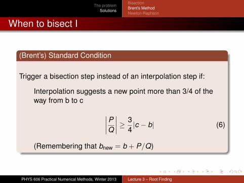
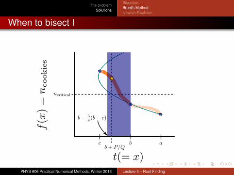
When to bisect I
(Brent’s) Standard Condition
Trigger a bisection step instead of an interpolation step if:
Interpolation suggests a new point more than 3/4 of theway from b to c ∣∣∣∣ P
Q
∣∣∣∣ ≥ 34|c − b| (6)
(Remembering that bnew = b + P/Q)
PHYS 606 Practical Numerical Methods, Winter 2013 Lecture 3 – Root Finding
The problemSolutions
BisectionBrent’s MethodNewton-Raphson
When to bisect I
PHYS 606 Practical Numerical Methods, Winter 2013 Lecture 3 – Root Finding
The problemSolutions
BisectionBrent’s MethodNewton-Raphson
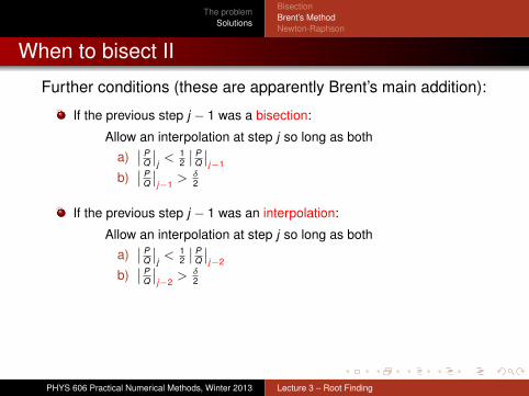
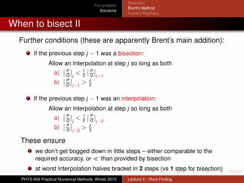
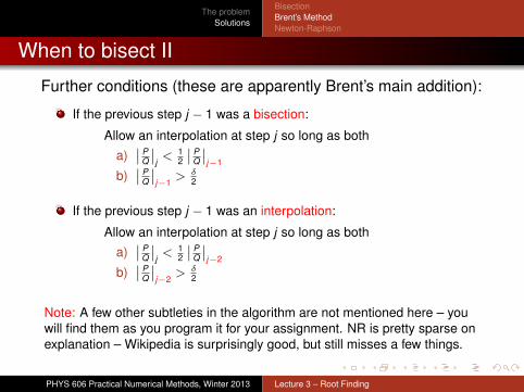
When to bisect II
Further conditions (these are apparently Brent’s main addition):
If the previous step j − 1 was a bisection:
Allow an interpolation at step j so long as botha)
∣∣ PQ
∣∣j< 1
2
∣∣ PQ
∣∣j−1
b)∣∣ P
Q
∣∣j−1
> δ2
If the previous step j − 1 was an interpolation:
Allow an interpolation at step j so long as botha)
∣∣ PQ
∣∣j< 1
2
∣∣ PQ
∣∣j−2
b)∣∣ P
Q
∣∣j−2
> δ2
PHYS 606 Practical Numerical Methods, Winter 2013 Lecture 3 – Root Finding
The problemSolutions
BisectionBrent’s MethodNewton-Raphson
When to bisect II
Further conditions (these are apparently Brent’s main addition):
If the previous step j − 1 was a bisection:
Allow an interpolation at step j so long as botha)
∣∣ PQ
∣∣j< 1
2
∣∣ PQ
∣∣j−1
b)∣∣ P
Q
∣∣j−1
> δ2
If the previous step j − 1 was an interpolation:
Allow an interpolation at step j so long as botha)
∣∣ PQ
∣∣j< 1
2
∣∣ PQ
∣∣j−2
b)∣∣ P
Q
∣∣j−2
> δ2
PHYS 606 Practical Numerical Methods, Winter 2013 Lecture 3 – Root Finding
These ensurewe don’t get bogged down in little steps – either comparable to therequired accuracy, or � than provided by bisection
at worst interpolation halves bracket in 2 steps (vs 1 step for bisection)
The problemSolutions
BisectionBrent’s MethodNewton-Raphson
When to bisect II
Further conditions (these are apparently Brent’s main addition):
If the previous step j − 1 was a bisection:
Allow an interpolation at step j so long as botha)
∣∣ PQ
∣∣j< 1
2
∣∣ PQ
∣∣j−1
b)∣∣ P
Q
∣∣j−1
> δ2
If the previous step j − 1 was an interpolation:
Allow an interpolation at step j so long as botha)
∣∣ PQ
∣∣j< 1
2
∣∣ PQ
∣∣j−2
b)∣∣ P
Q
∣∣j−2
> δ2
PHYS 606 Practical Numerical Methods, Winter 2013 Lecture 3 – Root Finding
Note: A few other subtleties in the algorithm are not mentioned here – youwill find them as you program it for your assignment. NR is pretty sparse onexplanation – Wikipedia is surprisingly good, but still misses a few things.
The problemSolutions
BisectionBrent’s MethodNewton-Raphson
Outline
1 The problem
2 SolutionsBisectionBrent’s MethodNewton-Raphson
PHYS 606 Practical Numerical Methods, Winter 2013 Lecture 3 – Root Finding
The problemSolutions
BisectionBrent’s MethodNewton-Raphson
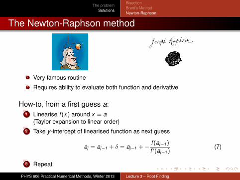
The Newton-Raphson method
Very famous routine
Requires ability to evaluate both function and derivative
How-to, from a first guess a:1 Linearise f (x) around x = a
(Taylor expansion to linear order)2 Take y -intercept of linearised function as next guess
aj = aj−1 + δ = aj−1 +− f (aj−1)
f ′(aj−1)(7)
3 Repeat
PHYS 606 Practical Numerical Methods, Winter 2013 Lecture 3 – Root Finding
The problemSolutions
BisectionBrent’s MethodNewton-Raphson
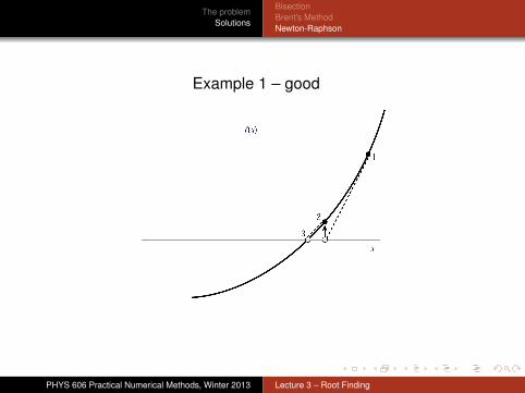
Example 1 – good
PHYS 606 Practical Numerical Methods, Winter 2013 Lecture 3 – Root Finding
The problemSolutions
BisectionBrent’s MethodNewton-Raphson
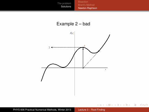
Example 2 – bad
PHYS 606 Practical Numerical Methods, Winter 2013 Lecture 3 – Root Finding
The problemSolutions
BisectionBrent’s MethodNewton-Raphson
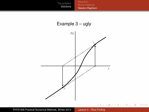
Example 3 – ugly
PHYS 606 Practical Numerical Methods, Winter 2013 Lecture 3 – Root Finding
The problemSolutions
BisectionBrent’s MethodNewton-Raphson
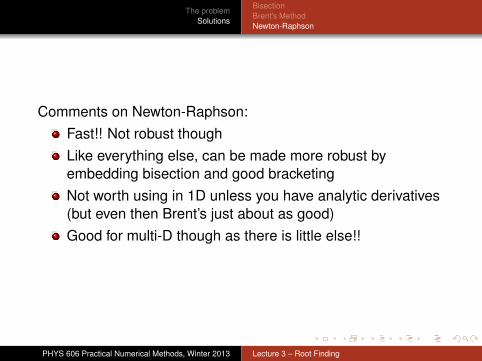
Comments on Newton-Raphson:Fast!! Not robust thoughLike everything else, can be made more robust byembedding bisection and good bracketingNot worth using in 1D unless you have analytic derivatives(but even then Brent’s just about as good)Good for multi-D though as there is little else!!
PHYS 606 Practical Numerical Methods, Winter 2013 Lecture 3 – Root Finding

The problemSolutions
BisectionBrent’s MethodNewton-Raphson
Housekeeping
Issues with Assignment 1?Next lecture: Random Numbers (Monday Jan 28)
PHYS 606 Practical Numerical Methods, Winter 2013 Lecture 3 – Root Finding