Elliptic partial differential equations. Poisson solvers.

LECTURE 9

1. Gravity force and the equations of hydrodynamics

Practical in Numerical Astronomy, SS 2012

11

1. Gravity force and the equations of hydrodynamics

2. Poisson equation versus Poisson integral

3. Numerical solution of the Poisson equation

4. Numerical integration of the Poisson integral

Lecturer

Eduard Vorobyov. Email: eduard.vorobiev@univie.ac.at

GRAVITY FORCE and THE EQUATIONS OF HYDRODYNAMICS

2

Although gravity is omnipresent in the Universe, its effect is often simplified or even neglected. However, there are situations when an accurate calculation of gravity is a necessity. In this context, two conceptually distinct descriptions of gravity are often used: external gravity and internal self-gravity.

1) External gravity is an additional external force acting onto the object under consideration. At the same time, the back reaction of the object onto the external perturber is neglected. The typical examples are the motion of gas and stars in the gravitational potential of the dark matter halo or the motion of a planet in the gravitational potential of a star.

2) Internal self-gravity or, simply, self-gravity acts as an intrinsic force, like that of the gas pressure, arising due to gravitational interaction of particles constituting the object under consideration. The

External gravity vs. self-gravity

arising due to gravitational interaction of particles constituting the object under consideration. The typical examples are the gravitational collapse of pre-stellar cores, formation of protostars and planets in protostellar disks or the growth of spiral structures in disk galaxies

-10 0 10

-10

0

10

Radia

l dis

tance (

kpc)

-10 0 10

1.1 Gyr

-10 0 10

1.3 Gyr1.2 Gyr

0

20

40

60

80

100

120

140

160

-10 0 10

1.4 Gyr

-10

0

10

Ra

dia

l d

ista

nce

(kp

c)

1.8 Gyr 2.2 Gyr 2.4 Gyr

0

20

40

60

80

100

120

140

160

2.6 Gyr

-10 0 10

-10

0

10

Rad

ial d

ista

nce (

kp

c)

3.0 Gyr

-10 0 10

3.3 Gyr

-10 0 10

3.7 Gyr

0

20

40

60

80

100

-10 0 10

4.1 Gyr

-500

0

500

Ra

dia

l d

ista

nce

(A

U)

-500

0

500

1000 0.1 Myr 0.3 Myr 0.5 Myr

-500 0 500

Radial distance (AU)-1000 -500 0 500

-1000

-500

0

500

0.9 Myr

0.91

-500 0 500 1000-500 0 500

-1-0.500.511.522.53

If gravity cannot be neglected, the equations of hydrodynamics need to be modified

to include the effect of gravitational acceleration g

gravity force

per unit volume

Equations of hydrodynamics in Cartesian coordinates (i,j = x,y,z)

viscous force

per unit volume

pressure force

per unit volume( )0i

i

u

t x

ρρ ∂∂+ =

∂ ∂

( ) 0ijP

u u u gπ

ρ ρ ρ∂∂ ∂ ∂

+ ⋅ + − − =

4

work per unit volume

per unit time due

to gravity force

( ) 0i i j i

j i j

u u u gt x x x

ρ ρ ρ+ ⋅ + − − =∂ ∂ ∂ ∂

( ) 0j i ji i i

j

E E P u u u gt x

π ρ∂ ∂

+ + − − = ∂ ∂

See Nigel’s lecture for more details

DERIVING THE POISSON EQUATION and POISSON INTEGRAL FROM NEWTON’S LAW OF GRAVITY

5

2

GMmF

r= -- scalar form of Newton’s law for two-body interaction

3| |

GMm= −F r

r

vector form of Newton’s law for two-body interaction, where r is

the position vector of a particle with mass m, and F is the gravity

force acting on that object from a particle with mass M. Note the

minus sign appearing due to the fact that r and F are pointed in

opposite directions.

m

M

r

F

Newton’s law of gravity for two-body interaction

6

3 3| | | |

GMm GMm= = − ⇒ = −F g r g r

r r

Applying 2nd Newton’s law, one gets the gravitational acceleration g

In the following slides, boldfaced values are vectors or tensors

31

( )( )

| |

Ni j

i

j i j

GM

=

= −∑r - r

g rr - r

total acceleration acting on

particle i from particles j=(1…N).i

ri

rj

j=1

j=2

j=N

gj=1

ri-rj

gj=2

gj=N

Newton’s law of gravity for many interacting bodies

7

3

3

( )( )( )

| |V

G dρ ′ ′

′= −′∫

r r - rg r r

r - r

acceleration acting at position vector r within

a continuous body with density ρ and volume V

r

′r3

3

3

d in Cartesian coordinates

d = in cylindrical coordinates

d sin in spherical coordinates

dx dy dz

dz dr r d

dr r d r d

ϕ

θ θ ϕ

′ ′ ′ ′=

′ ′ ′ ′ ′

′ ′ ′ ′ ′ ′ ′=

r

r

r

Gravitational potential

Gravity is the so-called central force whose magnitude only depends on the distance r between the

interacting objects and is directed along the line joining them.

Work done by the gravity force has a nice property such that it does not depend on the path but

only on the starting and finishing points. This allows us to define the gravitational potential Φas follows

[ ]2 2 2r r r

∂Φ= = = − = − Φ − Φ∫ ∫ ∫Fdr gdr dr The minus sign is due to

8

3

3where is the Nabla operator

( )( )( ) ( ) ,

| |V

G dρ ′ ′ ∂

′= −∇Φ = − ∇ =′ ∂∫

r r - rg r r r

r - r r

[ ]1 1 1

2 1( ) ( )r r r

A m m m r r∂Φ

= = = − = − Φ − Φ∂∫ ∫ ∫Fdr gdr drr

Gravitational potential is a scalar field in the sense that it takes scalar values but, at the same

time, is a function of the position vector. It has dimensions of energy per unit mass and is always

negative (due to attraction nature of the gravity force).

The minus sign is due to

the fact that Φ is negative

3

3

( )( )( )

| |V

G dρ ′ ′

′∇Φ =′∫

r r - rr r

r - r

3 3

1; 4 ( )

| | | | | |πδ

′−∇ = − ∇ =

′ ′− −

r r rr

r r r r r

proof can be done expanding these identities in Cartesian coordinates

applying the first identity … applying the second identity …

Deriving Poisson equation and Poisson integral

Let us use the following two vector identities

9

3

3

3 3

( )( )( )

| |

( ) ( )

| | | |

V

V V

G d

G d G d

ρ

ρ ρ

′ ′′∇Φ = =

′

′ ′′ ′= − ∇ = − ∇

′ ′− −

∫

∫ ∫

r r - rr r

r - r

r rr r

r r r r

3( )( )

| |V

G dρ ′

′Φ = −′−∫

rr r

r r

3

3

3

( )( )( ) ( )

| |

4 ( ) ( ) 4 ( )

V

G d

G d G

ρ

π ρ δ π ρ

′ ′′∇∇Φ = ∆Φ = ∇ =

′

′ ′ ′= =

∫

∫

r r - rr r r

r - r

r r - r r r

where is the Laplace operator

( ) 4 ( ),

Gπ ρ∆Φ =

∂ ∂∆ =

∂ ∂

r r

r r

… we arrive at the Poisson integral … we arrive at the Poisson equation

POISSON EQUATION - a prototype elliptic

partial differential equation

10

partial differential equation

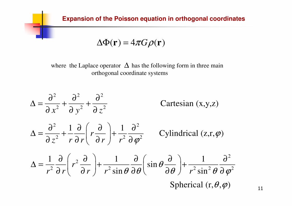
where the Laplace operator has the following form in three main

orthogonal coordinate systems

2 2 2

Cartesian (x,y,z)∂ ∂ ∂

∆ = + +

∆

( ) 4 ( )Gπ ρ∆Φ =r r

Expansion of the Poisson equation in orthogonal coordinates

11

2 2 2 Cartesian (x,y,z)

x y z∆ = + +

∂ ∂ ∂

2 2

2 2 2

1 1 Cylindrical (z,r, )r

z r r r rϕ

ϕ

∂ ∂ ∂ ∂∆ = + +

∂ ∂ ∂ ∂

22

2 2 2 2 2

1 1 1sin

sin sin

Spherical (r, , )

rr r r r r

θθ θ θ θ ϕ

θ ϕ

∂ ∂ ∂ ∂ ∂ ∆ = + +

∂ ∂ ∂ ∂ ∂

Classification of the Poisson equation

2 2 2

2 22 0, (1)

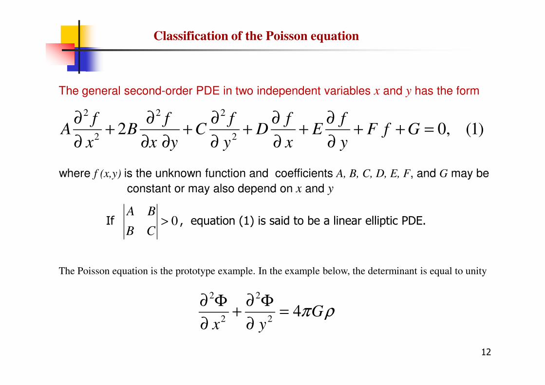
f f f f fA B C D E F f G

x x y y x y

∂ ∂ ∂ ∂ ∂+ + + + + + =

∂ ∂ ∂ ∂ ∂ ∂

where f (x,y) is the unknown function and coefficients A, B, C, D, E, F, and G may be

constant or may also depend on x and y

The general second-order PDE in two independent variables x and y has the form

If , equation (1) is said to be a linear elliptic PDE.

constant or may also depend on x and y

The Poisson equation is the prototype example. In the example below, the determinant is equal to unity

2 2

2 24 G

x yπ ρ

∂ Φ ∂ Φ+ =

∂ ∂

0A B

B C>

12

Elliptical PDEs are different from parabolic PDEs (e.g., diffusion equation) or

hyperbolic PDEs (wave equation, transport equation) in the sense that the latter are

the initial value problems while the former is the boundary value problem.

2 2

2 2

f f f

t x y

∂ ∂ ∂= +

∂ ∂ ∂

2 2 2

2 2 24 G

x y zπ ρ

∂ Φ ∂ Φ ∂ Φ+ + =

∂ ∂ ∂

x

y

t=t0

t=t1

Solving for the diffusion equation means advancing

the solution in time starting from the initial layer of

known values of f at t=t0. That is why this sort of

problems is called the initial value problem. Boundary

values also need to be known but only one layer at a time.

Solving for the Poisson equation means finding all the values

of the potential Φ inside the cube “at once” using pre-

calculated boundary values. Usually, one cannot march from

the outer boundary towards the center in the same sense as

the initial value problem can be integrated forward in time.

xy

z

Φ is known

at the cube

faces but is

unknown inside

the cube

Φ is known

NUMERICAL SOLUTION of the POISSON EQUATION

14

j=3

j=2

Discretization of the Poisson equation

dx

dy

1,2Φ

2 2

2 24 G

x yπ ρ

∂ Φ ∂ ΦΦ = + =

∂ ∂∆∆∆∆

1, ,

1/ 2

i j i j

ix dx

+

+

Φ − Φ∂Φ =

∂

Discretizing the first derivative

Suppose we need to find the gravitational potential on a mesh with 3 x 3 grid zones of equal size in each direction. The grid zone size is dx and dy in the x- and y-directions. The first step

would be to discretize the 2D Poisson equation.

15

1, , 1, , 1 , , 1

,2 2

2 24

i j i j i j i j i j i j

i jGdx dy

π ρ+ − + −Φ − Φ + Φ Φ − Φ + ΦΦ = + =∆∆∆∆

For a simple case of 2D Cartesian equidistant mesh we obtain a five-zone molecule

i=0 i=1 i=2 i=3

j=1

boundary

layer

21/ 2, 1/ 2,

2

i j i jx x

x dx

+ −

∂Φ ∂Φ −

∂ ∂∂ Φ =

∂

1 1/ 2,2x +

∂Φ

∂

boundary

value, Φ0,2

Discretizing the second derivative

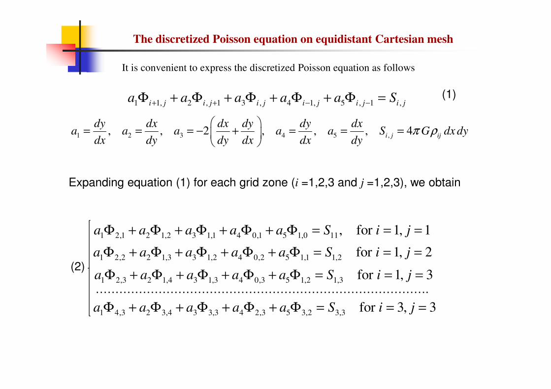
1 2 3 4 5 ,, , 2 , , , 4i j ij

dy dx dx dy dy dxa a a a a S G dx dy

dx dy dy dx dx dyπ ρ

= = = − + = = =

1 1, 2 , 1 3 , 4 1, 5 , 1 ,i j i j i j i j i j i ja a a a a S+ + − −Φ + Φ + Φ + Φ + Φ =

The discretized Poisson equation on equidistant Cartesian mesh

It is convenient to express the discretized Poisson equation as follows

Expanding equation (1) for each grid zone (i =1,2,3 and j =1,2,3), we obtain

(1)

1 2,1 2 1,2 3 1,1 4 0,1 5 1,0 11, for 1, 1a a a a a S i jΦ + Φ + Φ + Φ + Φ = = =

………………………………………………………………………….

1 4,3 2 3,4 3 3,3 4 2,3 5 3,2 3,3 for 3, 3a a a a a S i jΦ + Φ + Φ + Φ + Φ = = =

(2)1 2,2 2 1,3 3 1,2 4 0,2 5 1,1 1,2 for 1, 2a a a a a S i jΦ + Φ + Φ + Φ + Φ = = =

1 2,3 2 1,4 3 1,3 4 0,3 5 1,2 1,3 for 1, 3a a a a a S i jΦ + Φ + Φ + Φ + Φ = = =

Rearranging system (2) , we obtain nine equations for nine unknown Φi,j

3 1,1 2 1,2 1,3 1 2,1 2,2 2,3 3,1 3,2 3,3 11 4 0,1 5 1,00 0 0 0 0 0a a a S a aΦ + Φ + Φ + Φ + Φ + Φ + Φ + Φ + Φ = − Φ − Φ

………………………………………………………………………….

1,1 1,2 1,3 2,1 2,2 4 2,3 3,1 5 3,2 3 3,3 3,3 1 4,3 2 3,40 0 0 0 0 0a a a S a aΦ + Φ + Φ + Φ + Φ + Φ + Φ + Φ + Φ = − Φ − Φ

5 1,1 3 1,2 2 1,3 2,1 1 2,2 2,3 3,1 3,2 3,3 1,2 4 0,20 0 0 0 0a a a a S aΦ + Φ + Φ + Φ + Φ + Φ + Φ + Φ + Φ = − Φ

1,1 5 1,2 3 1,3 2,1 2,2 1 2,3 3,1 3,2 3,3 1,3 2 1,4 4 0,30 0 0 0 0 0a a a S a aΦ + Φ + Φ + Φ + Φ + Φ + Φ + Φ + Φ = − Φ − Φ

Discretized Poisson equation turns into a system of equations which can be expressed in the matrix form

A ΦΦΦΦ S

(3)

17

a3,b a2 0 a1 0 0 0b 0 0

a5 a3,b a2 0 a1 0 0 0b 0

0 a5 a3,b 0 0 a1 0 0 0b

a4 0 0 a3,b a2 0 a1 0 0

0 a4 0 a5 a3 a2 0 a1 0

0 0 a4 0 a5 a3,b 0 0 a1

0b 0 0 a4 0 0 a3,b a2 0

0 0b 0 0 a4 0 a5 a3,b a2

0 0 0b 0 0 a4 0 a5 a3,b

ΦΦΦΦ11111111

ΦΦΦΦ12121212

ΦΦΦΦ13131313

ΦΦΦΦ21212121

ΦΦΦΦ22222222

ΦΦΦΦ23232323

ΦΦΦΦ31313131

ΦΦΦΦ32323232

ΦΦΦΦ33333333

S11,b

S12,b

S13,b

S21,b

S22,b

S23,b

S31,b

S32,b

S33,b

A ΦΦΦΦ S

Boundary conditions

a3,b a2 0 a1 0 0 0b 0 0

a5 a3,b a2 0 a1 0 0 0b 0

0 a5 a3,b 0 0 a1 0 0 0b

a4 0 0 a3,b a2 0 a1 0 0

0 a4 0 a5 a3 a2 0 a1 0

ΦΦΦΦ11111111

ΦΦΦΦ12121212

ΦΦΦΦ13131313

ΦΦΦΦ21212121

ΦΦΦΦ22222222

S11,b

S12,b

S13,b

S21,b

S22,b

The subscript b indicates that these values can be affected by the boundary conditions

0 0 a4 0 a5 a3,b 0 0 a1

0b 0 0 a4 0 0 a3,b a2 0

0 0b 0 0 a4 0 a5 a3,b a2

0 0 0b 0 0 a4 0 a5 a3,b

ΦΦΦΦ22222222

ΦΦΦΦ23232323

ΦΦΦΦ31313131

ΦΦΦΦ32323232

ΦΦΦΦ33333333

S22,b

S23,b

S31,b

S32,b

S33,b

5 1,1 3 1,2 2 1,3 2,1 1 2,2 2,3 3,1 3,2 3,3 1,2 4 0,20 0 0 0 0a a a a S aΦ + Φ + Φ + Φ + Φ + Φ + Φ + Φ + Φ = − Φ

The value Φ0,2 needs to be specified a priori because we have 9 equation for 9 unknowns and

Φ0,2 is already the 10th unknown value.

Consider the second equation of system (3)

j=3

j=2

j=1

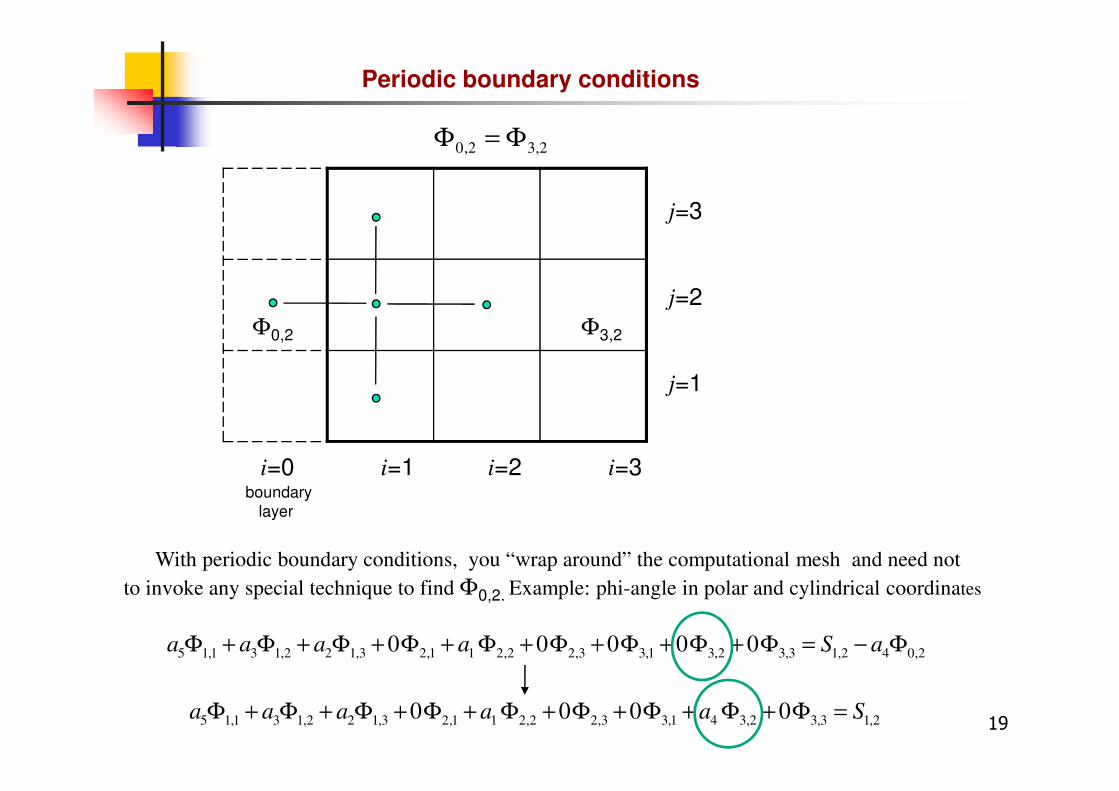
Periodic boundary conditions

Φ0,2 Φ3,2

0,2 3,2Φ = Φ

19

i=0 i=1 i=2 i=3

j=1

boundary

layer

With periodic boundary conditions, you “wrap around” the computational mesh and need not

to invoke any special technique to find Φ0,2. Example: phi-angle in polar and cylindrical coordinates

5 1,1 3 1,2 2 1,3 2,1 1 2,2 2,3 3,1 4 3,2 3,3 1,20 0 0 0a a a a a SΦ + Φ + Φ + Φ + Φ + Φ + Φ + Φ + Φ =

5 1,1 3 1,2 2 1,3 2,1 1 2,2 2,3 3,1 3,2 3,3 1,2 4 0,20 0 0 0 0a a a a S aΦ + Φ + Φ + Φ + Φ + Φ + Φ + Φ + Φ = − Φ

j=3

j=2

j=1

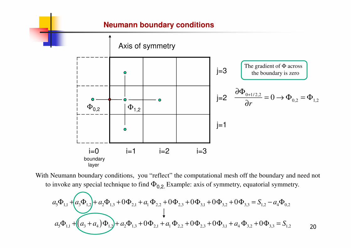
Axis of symmetry

0 1/ 2,2

0,2 1,20r

+∂Φ= → Φ = Φ

∂

Neumann boundary conditions

Φ0,2 Φ1,2

The gradient of Φ across

the boundary is zero

20

i=0 i=1 i=2 i=3

j=1

boundary

layer

With Neumann boundary conditions, you “reflect” the computational mesh off the boundary and need not

to invoke any special technique to find Φ0,2. Example: axis of symmetry, equatorial symmetry.

( )5 1,1 3 4 1,2 2 1,3 2,1 1 2,2 2,3 3,1 4 3,2 3,3 1,20 0 0 0a a a a a a SΦ + + Φ + Φ + Φ + Φ + Φ + Φ + Φ + Φ =

5 1,1 3 1,2 2 1,3 2,1 1 2,2 2,3 3,1 3,2 3,3 1,2 4 0,20 0 0 0 0a a a a S aΦ + Φ + Φ + Φ + Φ + Φ + Φ + Φ + Φ = − Φ

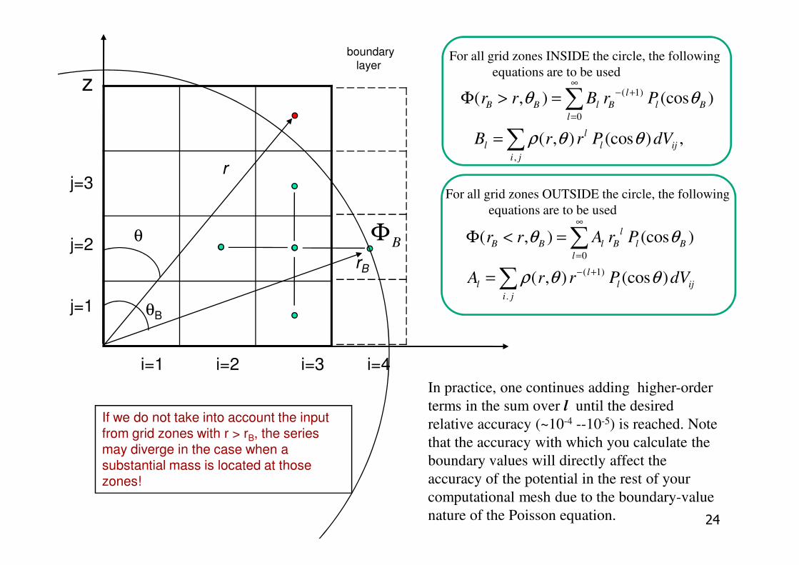
Dirichlet boundary conditions

j=3

j=2

boundary

layer

4,2BΦ ≡ Φ

21

i=1 i=2 i=3 i=4

j=1 rB

In the case that the boundary is neither periodic or reflective, multipole expansion is often used to

find the potential at the boundary. Example: outer boundaries of the computational domain (away

from reflection surfaces or axes of symmetry).

θΒ

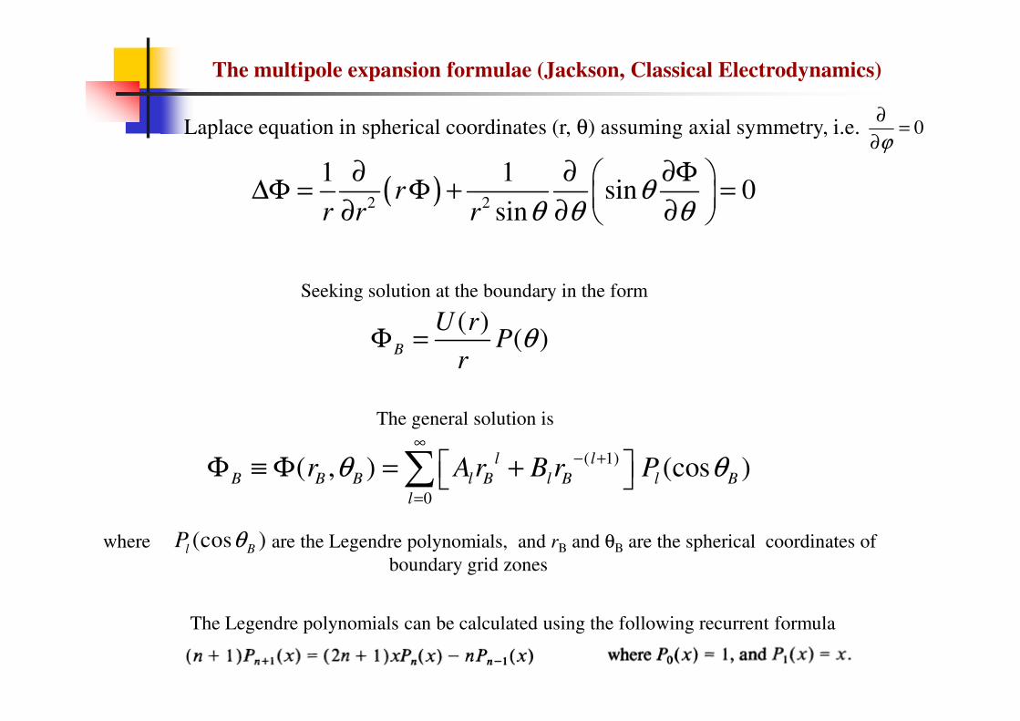
The multipole expansion formulae (Jackson, Classical Electrodynamics)

( )( )B

U rP

rθΦ =

( )2 2

1 1sin 0

sinr

r r rθ

θ θ θ

∂ ∂ ∂Φ ∆Φ = Φ + =

∂ ∂ ∂

Laplace equation in spherical coordinates (r, θ) assuming axial symmetry, i.e. 0ϕ

∂=

∂

Seeking solution at the boundary in the form

r

( 1)

0

( , ) (cos )l l

B B B l B l B l B

l

r A r B r Pθ θ∞

− +

=

Φ ≡ Φ = + ∑

where are the Legendre polynomials, and rB and θB are the spherical coordinates of

boundary grid zones

(cos )l B

P θ

The general solution is

The Legendre polynomials can be calculated using the following recurrent formula

( 1)

0 0

( , ) (cos ), ( , ) (cos )l l

B B l B l B B B l B l B

l l

r r B r P r r A r Pθ θ θ θ∞ ∞

− +

= =

Φ > = Φ < =∑ ∑

where B and A are the so-called interior and exterior multipole moments

( 1)

0

( , ) (cos )l l

B B B l B l B l B

l

r A r B r Pθ θ∞

− +

=

Φ ≡ Φ = + ∑

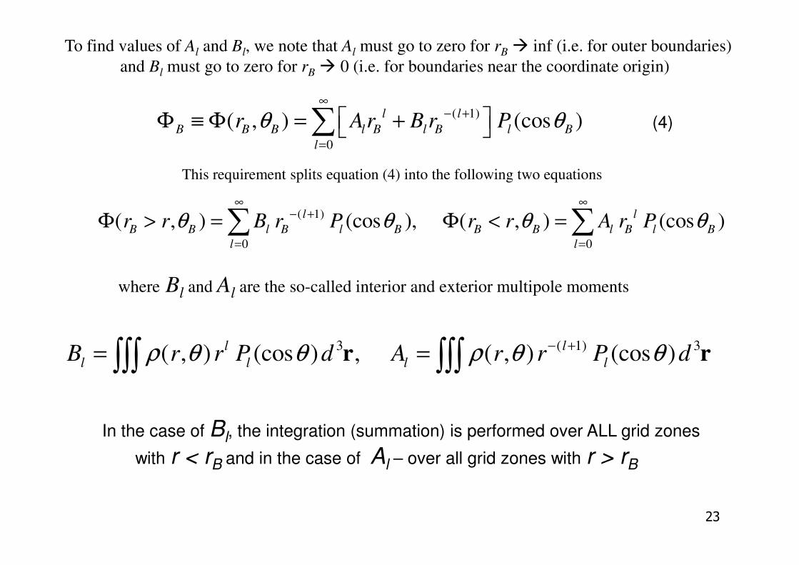
To find values of Al and Bl, we note that Al must go to zero for rB � inf (i.e. for outer boundaries)

and Bl must go to zero for rB � 0 (i.e. for boundaries near the coordinate origin)

This requirement splits equation (4) into the following two equations

(4)

23

where Bl and Al are the so-called interior and exterior multipole moments

3 ( 1) 3( , ) (cos ) , ( , ) (cos )l l

l l l lB r r P d A r r P dρ θ θ ρ θ θ− += =∫∫∫ ∫∫∫r r

In the case of Bl, the integration (summation) is performed over ALL grid zones

with r < rB and in the case of Al – over all grid zones with r > rB

j=3

j=2

boundary

layer

z

rB

BΦ

( 1)

0

,

( , ) (cos )

( , ) (cos ) ,

l

B B l B l B

l

l

l l ij

i j

r r B r P

B r r P dV

θ θ

ρ θ θ

∞− +

=

Φ > =

=

∑

∑r

θ0

( 1)

( , ) (cos )

( , ) (cos )

l

B B l B l B

l

l

l l ij

r r A r P

A r r P dV

θ θ

ρ θ θ

∞

=

− +

Φ < =

=

∑

∑

For all grid zones INSIDE the circle, the following

equations are to be used

For all grid zones OUTSIDE the circle, the following

equations are to be used

24

i=1 i=2 i=3 i=4

j=1

If we do not take into account the input from grid zones with r > rB, the series may diverge in the case when a substantial mass is located at those zones!

θB

In practice, one continues adding higher-order

terms in the sum over l until the desired

relative accuracy (~10-4 --10-5) is reached. Note

that the accuracy with which you calculate the

boundary values will directly affect the

accuracy of the potential in the rest of your

computational mesh due to the boundary-value

nature of the Poisson equation.

.

( , ) (cos )l l ij

i j

A r r P dVρ θ θ=∑

General strategy for solving the Poisson equation

Discretization and boundary conditions

Once the Poisson equation is properly discretized, the boundary conditions are specified, and

the boundary values of the potential are found, one needs to choose the fastest method for

solving the following matrix equation (i.e., a large system of linear equations)

×A Φ = S

Equidistant grid with periodic Non-equidistant grid with

25

Fast Fourier Transform • Alternative direction implicit method (best in 2D with

axial symmetry)

• Successive overrelaxation (best in 2D, slow in full 3D)

• Multigrid methods (fast only on Cartesian

geometry, slow on cylindrical and spherical

geometries)

Equidistant grid with periodic

boundary conditions

Non-equidistant grid with

any boundary conditions

For details on each method see:

1. Press, Teukolsky, Vitterling, Flannery: “Numerical Recipes in Fortran”.

2. Bodenheimer, Laughlin, Rozyczka, Yorke: “Numerical Methods in Astrophysics”.

The Poisson Integral

26

The Poisson Integral

3( )( )

V

G dρ ′

′Φ = −′∫

rr r

r - r

1 1

2 20 0

( , )( , )

( ) ( )

N N

l ml m

l ml l m m

M x yx y G

x x y y

− −′ ′

′ ′= = ′ ′

Φ = −− + −

∑∑

Let us consider a 2D Cartesian grid. Substituting the integral with a double sum , we obtain

Finding the gravitational potential using the Poisson integral

27x

y

l=0 l=1 l=2 l=N-1

m=N-1

m=2

m=1

m=0

Note that no boundary values of Φ are involved in

the summation. This is the fundamental advantage

of the Poisson Integral over the Poisson equation.

You need not to find the boundary values!

Where is the mass contained

in a grid zone

( , )l mM x y′ ′

( , )l m′ ′

1 1 1 1

, ,2 2 2 20 0 0 0( ) ( )

N N N N

l ml m l l m m l m

l m l m

MG G M

x l l y m m

− − − −′ ′

′ ′ ′ ′− −′ ′ ′ ′= = = =

Φ = − =′ ′∆ − + ∆ −

∑∑ ∑∑

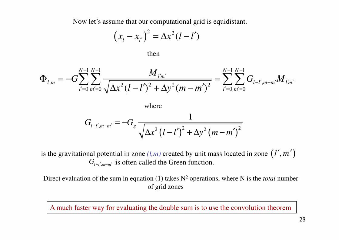
Now let’s assume that our computational grid is equidistant.

1G G= −

( )2 2 ( )

l lx x x l l′ ′− = ∆ −

then

where

28

( ) ( ), 2 22 2

1l l m m g

G Gx l l y m m

′ ′− − = −′ ′∆ − + ∆ −

( ),l m′ ′

A much faster way for evaluating the double sum is to use the convolution theorem

Direct evaluation of the sum in equation (1) takes N2 operations, where N is the total number

of grid zones

is the gravitational potential in zone (l,m) created by unit mass located in zone

is often called the Green function.,l l m mG ′ ′− −

1 1

, , ,

'

A B CN N

l m l m l l m m

l N m N

− −

′ ′ ′ ′− −′=− =−

= ∑ ∑

2 2ikl imnπ π− −)

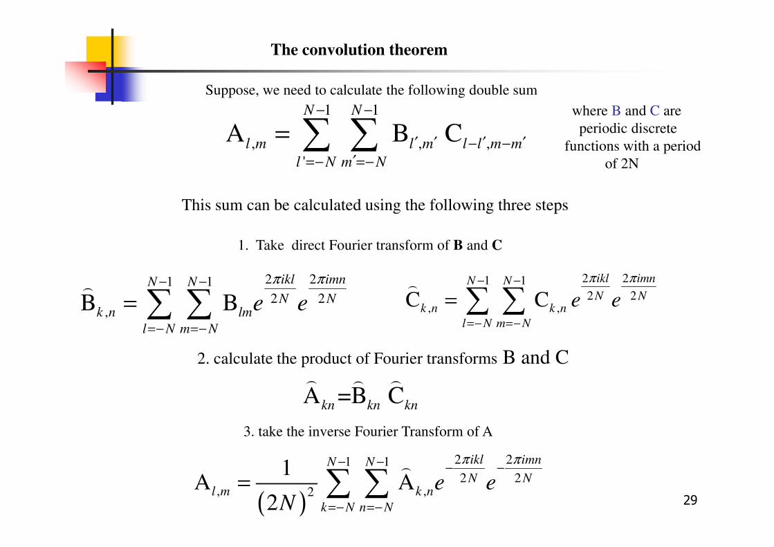
1. Take direct Fourier transform of B and C

This sum can be calculated using the following three steps

where B and C are

periodic discrete

functions with a period

of 2N

The convolution theorem

Suppose, we need to calculate the following double sum

2 21 1 ikl imnN N π π− −)

29

A =B Ckn kn kn

) ))

2 21 1

2 2,B B

ikl imnN N

N Nk n lm

l N m N

e e

π π− −

=− =−

= ∑ ∑)

2. calculate the product of Fourier transforms B and C

( )

2 21 1

2 2, ,2

1A A

2

ikl imnN N

N Nl m k n

k N n N

e eN

π π− − − −

=− =−

= ∑ ∑)

3. take the inverse Fourier Transform of A

2 21 1

2 2, ,C C

ikl imnN N

N Nk n k n

l N m N

e e

π π− −

=− =−

= ∑ ∑)

1 1

, , ,

'

A B CN N

l m l m l l m m

l N m N

− −

′ ′ ′ ′− −′=− =−

= ∑ ∑1 1

, ,

0 0

MN N

l m l m l l m m

l m

G− −

′ ′ ′ ′− −′ ′= =

Φ =∑∑

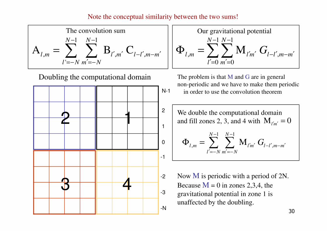
Doubling the computational domain

The convolution sum Our gravitational potential

The problem is that M and G are in general

non-periodic and we have to make them periodic

in order to use the convolution theorem

We double the computational domain

=

N-1

2

12

Note the conceptual similarity between the two sums!

30

1 1

, ,MN N

l m l m l l m m

l N m N

G− −

′ ′ ′ ′− −′ ′=− =−

Φ = ∑ ∑

Now M is periodic with a period of 2N.

Because M = 0 in zones 2,3,4, the

gravitational potential in zone 1 is

unaffected by the doubling.

We double the computational domain

and fill zones 2, 3, and 4 with M 0l m′ ′ =

1

0

-1

-2

-3

-N

12

3 4

Re-arranging the computational domain to make periodic

12

l=-N l=-3 l=-2 l=1 l=0 l=1 l=2 l=N-1

m=N-1

m=2

,l l m mG ′ ′− −

31

( ) ( ), 2 22 2

1l l m m g

G Gx l l y m m

′ ′− − = −′ ′∆ − +∆ −

12

3 4

40 50 60 70 80 90 100 90

m=1

m=0

m=-1

m=-2

m=-3

m=-N

We cannot simply set G to zero in zones

2,3,4 because it is the inverse distance.

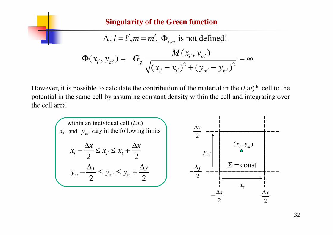
,At , , is not defined!l ml l m m′ ′= = Φ

However, it is possible to calculate the contribution of the material in the (l,m)th cell to the

potential in the same cell by assuming constant density within the cell and integrating over

the cell area

2 2

( , )( , )

( ) ( )

l ml m g

l l m m

M x yx y G

x x y y

′ ′′ ′

′ ′ ′ ′

Φ = − = ∞− + −

Singularity of the Green function

32

2

x∆

2

y∆

2 2

2 2

l l l

m m m

x xx x x

y yy y y

′

′

∆ ∆− ≤ ≤ +

∆ ∆− ≤ ≤ +

within an individual cell (l,m)

vary in the following limits

2

x∆−

2

y∆−

lx ′

my ′

( , )l mx y

and l mx y′ ′

constΣ =

2 2

y x

dx dy

∆ ∆

′ ′

and l l m m

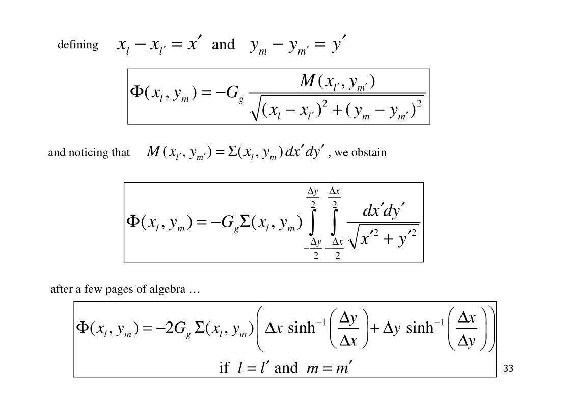
x x x y y y′ ′′ ′− = − =defining

( , ) ( , )l m l m

M x y x y dx dy′ ′ ′ ′= Σand noticing that , we obstain

2 2

( , )( , )

( ) ( )

l ml m g

l l m m

M x yx y G

x x y y

′ ′

′ ′

Φ = −− + −

33

after a few pages of algebra …

1 1( , ) 2 ( , ) sinh sinh

if and

l m g l m

y xx y G x y x y

x y

l l m m

− − ∆ ∆ Φ = − Σ ∆ + ∆ ∆ ∆

′ ′= =

2 2

2 2

2 2

( , ) ( , )l m g l m

y x

dx dyx y G x y

x y∆ ∆− −

′ ′Φ = − Σ

′ ′+∫ ∫

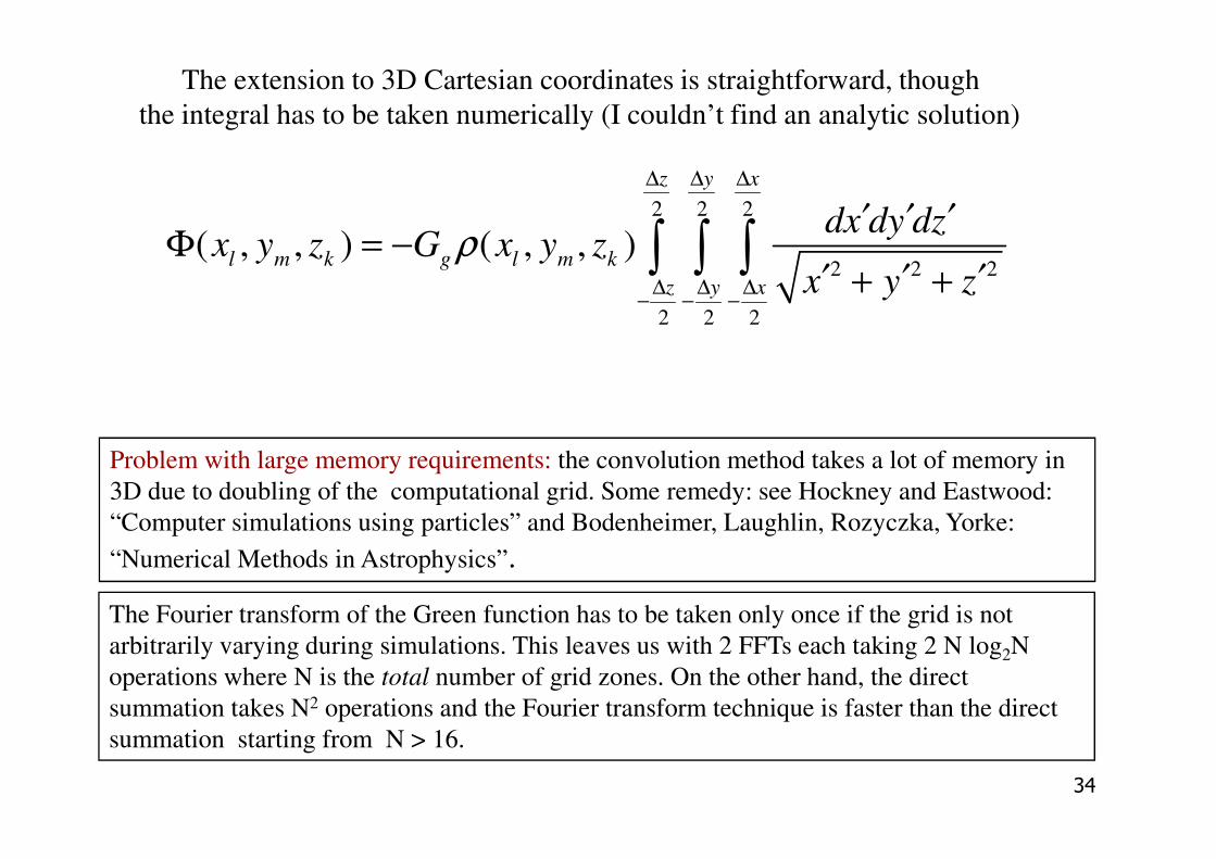
The extension to 3D Cartesian coordinates is straightforward, though

the integral has to be taken numerically (I couldn’t find an analytic solution)

2 2 2

2 2 2

2 2 2

( , , ) ( , , )

z y x

l m k g l m k

z y x

dx dy dzx y z G x y z

x y zρ

∆ ∆ ∆

∆ ∆ ∆− − −

′ ′ ′Φ = −

′ ′ ′+ +∫ ∫ ∫

34

Problem with large memory requirements: the convolution method takes a lot of memory in

3D due to doubling of the computational grid. Some remedy: see Hockney and Eastwood:

“Computer simulations using particles” and Bodenheimer, Laughlin, Rozyczka, Yorke:

“Numerical Methods in Astrophysics”.

The Fourier transform of the Green function has to be taken only once if the grid is not

arbitrarily varying during simulations. This leaves us with 2 FFTs each taking 2 N log2N

operations where N is the total number of grid zones. On the other hand, the direct

summation takes N2 operations and the Fourier transform technique is faster than the direct

summation starting from N > 16.

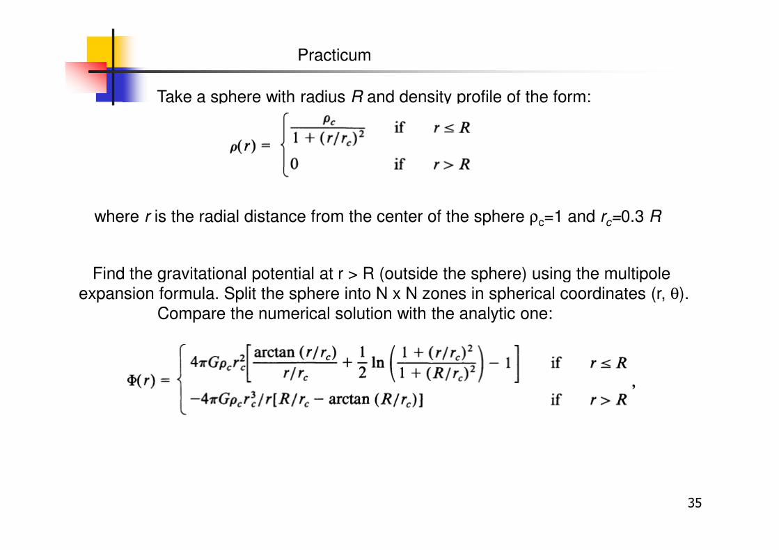
Practicum

Take a sphere with radius R and density profile of the form:

where r is the radial distance from the center of the sphere ρc=1 and rc=0.3 R

Find the gravitational potential at r > R (outside the sphere) using the multipole

35

Find the gravitational potential at r > R (outside the sphere) using the multipole

expansion formula. Split the sphere into N x N zones in spherical coordinates (r, θ).

Compare the numerical solution with the analytic one: