practical gamma-ray spectrometry
TRANSCRIPT
Practical Gamma-raySpectrometry
2nd Edition
Gordon R. GilmoreNuclear Training Services Ltd
Warrington, UK

Practical Gamma-raySpectrometry


Practical Gamma-raySpectrometry
2nd Edition
Gordon R. GilmoreNuclear Training Services Ltd
Warrington, UK
Copyright © 2008 John Wiley & Sons Ltd, The Atrium, Southern Gate, Chichester,West Sussex PO19 8SQ, England
Telephone �+44� 1243 779777
Email (for orders and customer service enquiries): [email protected] our Home Page on www.wiley.com
All Rights Reserved. No part of this publication may be reproduced, stored in a retrieval system or transmitted in any form or by any means,electronic, mechanical, photocopying, recording, scanning or otherwise, except under the terms of the Copyright, Designs and Patents Act 1988or under the terms of a licence issued by the Copyright Licensing Agency Ltd, 90 Tottenham Court Road, London W1T 4LP, UK, without thepermission in writing of the Publisher. Requests to the Publisher should be addressed to the Permissions Department, John Wiley & Sons Ltd,The Atrium, Southern Gate, Chichester, West Sussex PO19 8SQ, England, or emailed to [email protected], or faxed to (+44) 1243 770620.
Designations used by companies to distinguish their products are often claimed as trademarks. All brand names and product names used in thisbook are trade names, service marks, trademarks or registered trademarks of their respective owners. The Publisher is not associated with anyproduct or vendor mentioned in this book.
This publication is designed to provide accurate and authoritative information in regard to the subject matter covered. It is sold on theunderstanding that the Publisher is not engaged in rendering professional services. If professional advice or other expert assistance is required,the services of a competent professional should be sought.
The Publisher, and the Author make no representations or warranties with respect to the accuracy or completeness of the contents of this workand specifically disclaim all warranties, including without limitation any implied warranties of fitness for a particular purpose. The advice andstrategies contained herein may not be suitable for every situation. In view of ongoing research, equipment modifications, changes ingovernmental regulations, and the constant flow of information relating to the use of experimental reagents, equipment, and devices, the readeris urged to review and evaluate the information provided in the package insert or instructions for each chemical, piece of equipment, reagent, ordevice for, among other things, any changes in the instructions or indication of usage and for added warnings and precautions. The fact that anorganization or Website is referred to in this work as a citation and/or a potential source of further information does not mean that the author orthe publisher endorses the information the organization or Website may provide or recommendations it may make. Further, readers should beaware that Internet Websites listed in this work may have changed or disappeared between when this work was written and when it is read. Nowarranty may be created or extended by any promotional statements for this work. Neither the Publisher nor the Author shall be liable for anydamages arising herefrom.
Other Wiley Editorial Offices
John Wiley & Sons Inc., 111 River Street, Hoboken, NJ 07030, USA
Jossey-Bass, 989 Market Street, San Francisco, CA 94103-1741, USA
Wiley-VCH Verlag GmbH, Boschstr. 12, D-69469 Weinheim, Germany
John Wiley & Sons Australia Ltd, 42 McDougall Street, Milton, Queensland 4064, Australia
John Wiley & Sons (Asia) Pte Ltd, 2 Clementi Loop #02-01, Jin Xing Distripark, Singapore 129809
John Wiley & Sons Ltd, 6045 Freemont Blvd, Mississauga, Ontaria, L5R 4J3, Canada
Wiley also publishes its books in a variety of electronic formats. Some content that appears in print may not be available in electronic books.
Library of Congress Cataloging in Publication Data
Gilmore, Gordon.Practical gamma-ray spectrometry. — 2nd ed. / Gordon Gilmore.
p. cm.Includes bibliographical references and index.ISBN 978-0-470-86196-7 (cloth : alk. paper)1. Gamma ray spectrometry—Handbooks, manuals, etc. I. Title.QC793.5.G327G55 2008537.5′352—dc22
2007046837
British Library Cataloguing in Publication Data
A catalogue record for this book is available from the British Library
ISBN 978-0-470-86196-7
Typeset in 9/11pt Times by Integra Software Services Pvt. Ltd, Pondicherry, IndiaPrinted and bound in Great Britain by Antony Rowe Ltd, Chippenham, Wiltshire

Dedication
To my friends and family who, I suspect, never really believed I would get this finished,and to the publishers who patiently tolerated many delays before I did so


Contents
Preface to the Second Edition xv
Preface to the First Edition xvii
Internet Resources within the Book xix
1 Radioactive Decay and the Origin ofGamma and X-Radiation 11.1 Introduction 11.2 Beta Decay 2
1.2.1 �− or negatron decay 31.2.2 �+ or positron decay 51.2.3 Electron capture (EC) 61.2.4 Multiple stable isotopes 7
1.3 Alpha Decay 71.4 Spontaneous Fission (SF) 81.5 Minor Decay Modes 81.6 Gamma Emission 8
1.6.1 The electromagnetic spectrum 91.6.2 Some properties of nuclear
transitions 91.6.3 Lifetimes of nuclear energy
levels 101.6.4 Width of nuclear energy levels 101.6.5 Internal conversion 111.6.6 Abundance, yield and
emission probability 111.6.7 Ambiguity in assignment of
nuclide identity 111.7 Other Sources of Photons 12
1.7.1 Annihilation radiation 121.7.2 Bremsstrahlung 131.7.3 Prompt gammas 131.7.4 X-rays 13
1.8 The Mathematics of Decay andGrowth of Radioactivity 151.8.1 The decay equation 151.8.2 Growth of activity in reactors 161.8.3 Growth of activity from decay
of a parent 171.9 The Chart of the Nuclides 19
1.9.1 A source of nuclear data 19
1.9.2 A source of genericinformation 20
Practical Points 22Further Reading 23
2 Interactions of Gamma Radiation withMatter 252.1 Introduction 252.2 Mechanisms of Interaction 25
2.2.1 Photoelectric absorption 272.2.2 Compton scattering 282.2.3 Pair production 29
2.3 Total Attenuation Coefficients 292.4 Interactions within the Detector 30
2.4.1 The very large detector 302.4.2 The very small detector 312.4.3 The ‘real’ detector 322.4.4 Summary 32
2.5 Interactions within the Shielding 332.5.1 Photoelectric interactions 332.5.2 Compton scattering 342.5.3 Pair production 35
2.6 Bremsstrahlung 352.7 Attenuation of Gamma Radiation 362.8 The Design of Detector Shielding 36Practical Points 38Further Reading 38
3 Semiconductor Detectors for Gamma-RaySpectrometry 393.1 Introduction 393.2 Semiconductors and Gamma-Ray
Detection 403.2.1 The band structure of solids 403.2.2 Mobility of holes 403.2.3 Creation of charge carriers by
gamma radiation 413.2.4 Suitable semiconductors for
gamma-ray detectors 413.2.5 Newer semiconductor materials 42
3.3 The Nature of Semiconductors 43
viii Contents
3.4 The Manufacture of GermaniumDetectors 453.4.1 Introduction 453.4.2 The manufacturing process 453.4.3 Lithium-drifted detectors 473.4.4 The detector configurations
available 473.4.5 Absorption in detector caps
and dead layers 473.4.6 Detectors for low-energy
measurements 493.4.7 Well detectors 49
3.5 Detector Capacitance 493.5.1 Microphonic noise 50
3.6 Charge Collection in Detectors 503.6.1 Charge collection time 503.6.2 Shape of the detector pulse 513.6.3 Timing signals from
germanium detectors 523.6.4 Electric field variations across
the detector 523.6.5 Removing weak field regions
from detectors 533.6.6 Trapping of charge carriers 533.6.7 Radiation damage 54
3.7 Packaging of Detectors 553.7.1 Construction of the detector
mounting 553.7.2 Exotic detectors 573.7.3 Loss of coolant 583.7.4 Demountable detectors 583.7.5 Customer repairable detectors 583.7.6 Electrical cooling of detectors 59
Practical Points 59Further Reading 59
4 Electronics for Gamma-Ray Spectrometry 614.1 The General Electronic System 61
4.1.1 Introduction 614.1.2 Electronic noise and its
implications for spectrumresolution 62
4.1.3 Pulse shapes ingamma spectrometry systems 63
4.1.4 Impedance – inputs and outputs 644.1.5 The impedance of cabling 644.1.6 Impedance matching 65
4.2 Detector Bias Supplies 664.3 Preamplifiers 66
4.3.1 Resistive feedbackpreamplifiers 67
4.3.2 Reset preamplifiers 69
4.3.3 The noise contribution ofpreamplifiers 69
4.3.4 The rise time ofpreamplifiers 70
4.4 Amplifiers and Pulse Processors 704.4.1 The functions of the
amplifier 704.4.2 Pulse shaping 714.4.3 The optimum pulse shape 724.4.4 The optimum pulse shaping
time constant 734.4.5 The gated integrator
amplifier 744.4.6 Pole-zero cancellation 754.4.7 Baseline shift 764.4.8 Pile-up rejection 774.4.9 Amplifier gain and overview 78
4.5 Resolution Enhancement 804.5.1 New semiconductor
materials 804.6 Multichannel Analysers and their
Analogue-to-Digital Converters 814.6.1 Introduction 814.6.2 Pulse range selection 824.6.3 The ADC input gate 834.6.4 The ADC 844.6.5 MCA conversion time and
dead time 864.6.6 Choosing an ADC 874.6.7 Linearity in MCAs 884.6.8 Optimum spectrum size 894.6.9 MCA terms and definitions 894.6.10 Arrangement of the MCA
function 914.6.11 Simple MCA analysis
functions 914.7 Live Time Correction and Loss-Free
Counting 924.7.1 Live time clock correction 924.7.2 The Gedcke–Hale method 924.7.3 Use of a pulser 924.7.4 Loss-free counting (LFC) 934.7.5 MCA throughput 94
4.8 Spectrum Stabilization 944.8.1 Analogue stabilization 954.8.2 Digital stabilization 95
4.9 Coincidence and AnticoincidenceGating 96
4.10 Multiplexing and Multiscaling 964.11 Digital Pulse Processing Systems 97Practical Points 98Further Reading 99
Contents ix
5 Statistics of Counting 1015.1 Introduction 101
5.1.1 Statistical statements 1015.2 Counting Distributions 102
5.2.1 The binomial distribution 1025.2.2 The Poisson and Gaussian
distributions 1045.3 Sampling Statistics 104
5.3.1 Confidence limits 1055.3.2 Combining the results from
different measurements 1075.3.3 Propagation of uncertainty 108
5.4 Peak Area Measurement 1085.4.1 Simple peak integration 1095.4.2 Peaked-background
correction 1115.5 Optimizing Counting Conditions 111
5.5.1 Optimum background width 1115.5.2 Optimum spectrum size 1125.5.3 Optimum counting time 113
5.6 Counting Decision Limits 1145.6.1 Critical limit �LC� 1145.6.2 Upper limit �LU� 1165.6.3 Confidence limits 1175.6.4 Detection limit �LD� 1175.6.5 Determination limit �LQ� 1185.6.6 Other calculation options 1185.6.7 Minimum detectable activity
(MDA) 1195.6.8 Uncertainty of the �LU� and
MDA 1205.6.9 An example by way of
summary 1205.7 Special Counting Situations 121
5.7.1 Non-Poisson counting 1215.7.2 Low numbers of counts 1215.7.3 Non-Poisson statistics due to
pile-up rejection and loss-freecounting 122
5.8 Uncertainty Budgets 1235.8.1 Introduction 1235.8.2 Accuracy and precision 1245.8.3 Types of uncertainty 1245.8.4 Types of distribution 1245.8.5 Uncertainty on sample
preparation 1245.8.6 Counting uncertainties 1255.8.7 Calibration uncertainties 1265.8.8 An example of an uncertainty
budget 126Practical Points 128Further Reading 128
6 Resolution: Origins and Control 1316.1 Introduction 1316.2 Charge Production – �P 133
6.2.1 Germanium versus silicon 1336.2.2 Germanium versus sodium
iodide 1346.2.3 Temperature dependence of
resolution 1346.3 Charge Collection – �C 134
6.3.1 Mathematical form of �C 1356.4 Electronic Noise – �E 136
6.4.1 Parallel noise 1366.4.2 Series noise 1376.4.3 Flicker noise 1376.4.4 Total electronic noise and
shaping time 1376.5 Resolving the Peak Width Calibration 138Practical Points 141Further Reading 141References 141
7 Spectrometer Calibration 1437.1 Introduction 1437.2 Reference Data for Calibration 1437.3 Sources for Calibration 1447.4 Energy Calibration 144
7.4.1 Errors in peak energydetermination 146
7.5 Peak Width Calibration 1477.5.1 Factors affecting peak width 1477.5.2 Algorithms for peak width
estimation 1477.5.3 Estimation of the peak height 1497.5.4 Anomalous peak widths 149
7.6 Efficiency Calibration 1507.6.1 Which efficiency? 1507.6.2 Full-energy peak efficiency 1517.6.3 Are efficiency calibration
curves necessary? 1527.6.4 The effect of
source-to-detector distance 1527.6.5 Calibration errors due to
difference in sample geometry 1537.6.6 An empirical correction for
sample height 1547.6.7 Effect of source density on
efficiency 1557.6.8 Efficiency loss due to
random summing (pile-up) 1587.6.9 True coincidence summing 1597.6.10 Corrections for radioactive
decay 159

x Contents
7.6.11 Electronic timing problems 1607.7 Mathematical Efficiency Calibration 160
7.7.1 ISOCS 1617.7.2 LabSOCS 1627.7.3 Other programs 162
Practical Points 162Further Reading 163
8 True Coincidence Summing 1658.1 Introduction 1658.2 The Origin of Summing 1668.3 Summing and Solid Angle 1668.4 Spectral Evidence of Summing 1678.5 Validity of Close Geometry
Calibrations 1688.5.1 Efficiency calibration using
QCYK mixed nuclidesources 168
8.6 Summary 1718.7 Summing in Environmental
Measurements 1718.8 Achieving Valid
Close Geometry EfficiencyCalibrations 172
8.9 TCS, Geometry and Composition 1748.10 Achieving ‘Summing-free’
measurements 1758.10.1 Using the ‘interpolative fit’
to correct for TCS 1758.10.2 Comparative activity
measurements 1758.10.3 Using correction
factors derived fromefficiency calibration curves 176
8.10.4 Correction of results using‘bodged’ nuclear data 176
8.11 Mathematical Summing Corrections 1768.12 Software for Correction of TCS 178
8.12.1 GESPECOR 1798.12.2 Calibrations using
summing nuclides 1798.12.3 TCS correction in spectrum
analysis programs 179Practical Points 180Further Reading 180
9 Computer Analysis of Gamma-RaySpectra 1839.1 Introduction 1839.2 Methods of Locating Peaks
in the Spectrum 1859.2.1 Using regions-of-interest 185
9.2.2 Locating peaks usingchannel differences 185
9.2.3 Derivative peak searches 1859.2.4 Peak searches using
correlation methods 1869.2.5 Checking the acceptability
of peaks 1879.3 Library Directed Peak Searches 1879.4 Energy Calibration 1889.5 Estimation of the Peak Centroid 1899.6 Peak Width Calibration 1899.7 Determination of the Peak Limits 191
9.7.1 Using the width calibration 1929.7.2 Individual peak width
estimation 1929.7.3 Limits determined by a
moving average minimum 1929.8 Measurements of Peak Area 1929.9 Full Energy Peak Efficiency
Calibration 1939.10 Multiplet Peak Resolution
by Deconvolution 1959.11 Peak Stripping as a Means
of Avoiding Deconvolution 1969.12 The Analysis of the Sample Spectrum 197
9.12.1 Peak location andmeasurement 198
9.12.2 Corrections to the peakarea for peakedbackground 198
9.12.3 Upper limits andminimum detectableactivity 198
9.12.4 Comparative activityestimations 199
9.12.5 Activity estimations usingefficiency curves 199
9.12.6 Corrections independentof the spectrometer 199
9.13 Nuclide Identification 2009.13.1 Simple use of look-up
tables 2009.13.2 Taking into account other
peaks 2009.14 The Final Report 2009.15 Setting Up Nuclide and Gamma-Ray
Libraries 2019.16 Buying Spectrum Analysis Software 2029.17 The Spectrum Analysis Programs
Referred to in the Text 202Practical Points 202Further Reading 203

Contents xi
10 Scintillation Spectrometry 20510.1 Introduction 20510.2 The Scintillation Process 20510.3 Scintillation Activators 20610.4 Life time of Excited States 20610.5 Temperature Variation of the
Scintillator Response 20710.6 Scintillator Detector Materials 207
10.6.1 Sodium iodide – NaI(Tl) 20710.6.2 Bismuth germanate –
BGO 20810.6.3 Caesium iodide –
CsI(Tl) and CsI(Na) 20910.6.4 Undoped caesium
iodide – CsI 20910.6.5 Barium fluoride – BaF2 20910.6.6 Caesium fluoride – CsF 21010.6.7 Lanthanum halides –
LaCl3(Ce) and LaBr3(Ce) 21010.6.8 Other new scintillators 210
10.7 Photomultiplier Tubes 21110.8 The Photocathode 21110.9 The Dynode Electron Multiplier
Chain 21210.10 Photodiode Scintillation
Detectors 21210.11 Construction of the Complete
Detector 21310.11.1 Detector shapes 21310.11.2 Optical coupling of the
scintillator to thephotomultiplier 213
10.12 The Resolution of ScintillationSystems 21410.12.1 Statistical uncertainties
in the detection process 21510.12.2 Factors associated with
the scintillator crystal 21510.12.3 The variation of
resolution withgamma-ray energy 216
10.13 Electronics for ScintillationSystems 21610.13.1 High-voltage supply 21610.13.2 Preamplifiers 21710.13.3 Amplifiers 21710.13.4 Multi-channel analysers
and spectrum analysis 21710.14 Comparison of Sodium Iodide and
Germanium Detectors 218Practical Points 219Further Reading 219
11 Choosing and Setting up a Detector, andChecking its Specifications 22111.1 Introduction 22111.2 Setting up a Germanium Detector
System 22211.2.1 Installation – the detector
environment 22211.2.2 Liquid nitrogen supply 22311.2.3 Shielding 22411.2.4 Cabling 22411.2.5 Installing the detector 22511.2.6 Preparation for
powering-up 22511.2.7 Powering-up and initial
checks 22611.2.8 Switching off the system 228
11.3 Optimizing the ElectronicSystem 22811.3.1 General considerations 22811.3.2 DC level adjustment and
baseline noise 22811.3.3 Setting the conversion
gain and energy range 22811.3.4 Pole-zero (PZ) cancellation 23011.3.5 Incorporating a pulse
generator 23111.3.6 Baseline restoration
(BLR) 23111.3.7 Optimum time constant 231
11.4 Checking the Manufacturer’sSpecification 23211.4.1 The Manufacturer’s
Specification Sheet 23211.4.2 Detector resolution and
peak shape 23311.4.3 Detector efficiency 23511.4.4 Peak-to-Compton (P/C)
ratio 23711.4.5 Window thickness index 23811.4.6 Physical parameters 238
Practical Points 238Further Reading 238
12 Troubleshooting 23912.1 Fault-Finding 239
12.1.1 Equipment required 23912.1.2 Fault-finding guide 240
12.2 Preamplifier Test Point andLeakage Current 24312.2.1 Resistive feedback (RF)
preamplifiers 243
xii Contents
12.2.2 Transistor reset andpulsed optical resetpreamplifiers 244
12.3 Thermal Cycling of the Detector 24412.3.1 The origin of the
problem 24412.3.2 The thermal cycling
procedure 24512.3.3 Frosted detector
enclosure 24612.4 Ground Loops, Pick-up and
Microphonics 24612.4.1 Ground loops 24612.4.2 Electromagnetic pick-up 24712.4.3 Microphonics 249
Practical Points 250Further Reading 250
13 Low Count Rate Systems 25113.1 Introduction 25113.2 Counting with High Efficiency 253
13.2.1 MDA: efficiency andresolution 253
13.2.2 MDA: efficiency,background and countingperiod 253
13.3 The Effect of Detector Shape 25713.3.1 Low energy measurements 25713.3.2 Well detectors 25813.3.3 Sample quantity and
geometry 25913.4 Low Background Systems 262
13.4.1 The background spectrum 26313.4.2 Low background
detectors 26313.4.3 Detector shielding 26513.4.4 The graded shield 26513.4.5 Airborne activity 26613.4.6 The effect of cosmic
radiation 26613.4.7 Underground measurements 269
13.5 Active Background Reduction 27013.5.1 Compton suppression
systems 27013.5.2 Veto guard detectors 273
13.6 Ultra-Low-Level Systems 273Practical Points 276Further Reading 276
14 High Count Rate Systems 27914.1 Introduction 27914.2 Detector Throughput 280
14.3 Preamplifiers for HighCount Rate 28114.3.1 Energy rate saturation 28114.3.2 Energy resolution 28314.3.3 Dead time 283
14.4 Amplifiers 28314.4.1 Time constants and pile-up 28414.4.2 The gated integrator 28414.4.3 Pole zero correction 28514.4.4 Amplifier stability – peak
shift 28514.4.5 Amplifier stability –
resolution 28514.4.6 Overload recovery 286
14.5 Digital Pulse Processing 28614.6 The ADC and MCA 28814.7 Dead Times and Throughput 288
14.7.1 Extendable andnon-extendable dead time 289
14.7.2 Gated integrators 29014.7.3 DSP systems 29114.7.4 Theory versus practice 291
14.8 System Checks 292Practical Points 293Further Reading 293
15 Ensuring Quality in Gamma-RaySpectrometry 29515.1 Introduction 29515.2 Nuclear Data 29615.3 Radionuclide Standards 29615.4 Maintaining Confidence in the
Equipment 29715.4.1 Setting up and
maintenance procedures 29715.4.2 Control charts 29815.4.3 Setting up a control chart 299
15.5 Gaining Confidence in the SpectrumAnalysis 30115.5.1 Test spectra 30115.5.2 Computer-generated test
spectra 30215.5.3 Test spectra created by
counting 30615.5.4 Assessing
spectrum analysisperformance 307
15.5.5 Intercomparison exercises 31015.5.6 Assessment of
intercomparison exercises 31115.6 Maintaining Records 31115.7 Accreditation 312

Contents xiii
Practical Points 313Further Reading 313Internet Sources of Information 314
16 Gamma Spectrometry of NaturallyOccurring Radioactive Materials(NORM) 31516.1 Introduction 31516.2 The NORM Decay Series 315
16.2.1 The uranium series – 238U 31616.2.2 The actinium series – 235U 31616.2.3 The thorium series – 232Th 31716.2.4 Radon loss 31716.2.5 Natural disturbance of the
decay series 31816.3 Gamma Spectrometry of the NORM
Nuclides 31816.3.1 Measurement of 7Be 31816.3.2 Measurement of 40K 31816.3.3 Gamma spectrometry of
the uranium/thorium seriesnuclides 318
16.3.4 Allowance for naturalbackground 319
16.3.5 Resolution of the 186 keVpeak 319
16.3.6 Other spectralinterferences and summing 322
16.4 Nuclear Data of the NORM Nuclides 32416.5 Measurement of Chemically
Modified NORM 32416.5.1 Measurement of separated
uranium 32516.5.2 Measurement of separated
thorium 32516.5.3 ‘Non-natural’ thorium 32616.5.4 Measurement of gypsum –
a cautionary tale 32716.5.5 General observations 328
Further Reading 328
17 Applications 32917.1 Gamma Spectrometry and the CTBT 329
17.1.1 Background 32917.1.2 The global verification
regime 32917.1.3 Nuclides released in a
nuclear explosion 33017.1.4 Measuring the
radionuclides 33117.1.5 Current status 332
17.2 Gamma Spectrometry of NuclearIndustry Wastes 33317.2.1 Measurement of
isotopically modifieduranium 333
17.2.2 Measurement oftransuranic nuclides 333
17.2.3 Waste drum scanning 33417.3 Safeguards 335
17.3.1 Enrichment meters 33617.3.2 Plutonium spectra 33617.3.3 Fresh and aged samples 33817.3.4 Absorption of gamma-rays 33817.3.5 Hand-held monitors 338
17.4 PINS – Portable Isotopic NeutronSpectrometry 340
Further Reading 340
Appendix A: Sources of Information 343A.1 Introduction 343A.2 Nuclear Data 343
A.2.1 Recent developments inthe distribution of nucleardata 344
A.2.2 On line internet sources ofgamma-ray emission data 345
A.2.3 Off-line sources ofgamma-ray emission data 346
A.2.4 Nuclear data in print 346A.3 Internet Sources of Other Nuclear
Data 347A.4 Chemical Information 347A.5 Miscellaneous Information 348A.6 Other Publications in print 348
Appendix B: Gamma- and X-Ray Standardsfor Detector Calibration 351
Appendix C: X-Rays Routinely Found inGamma Spectra 359
Appendix D: Gamma-Ray Energies in theDetector Background and theEnvironment 361
Appendix E: Chemical Names, Symbols andRelative Atomic Masses of theElements 365
Glossary 369
Index 381


Preface to the Second Edition
During 2005, while this second edition was beingprepared, I was totally unprepared to receive a tele-phone call that my co-author on the first edition, JohnHemingway, was seriously ill after suffering a brain-haemorrhage. Only a few days later, on 5th September,he passed away. My original, and obvious, intent wasto update the sections allocated to John and myself andpublish this second edition as ‘Gilmore and Hemingway’.That intent was frustrated by contractual difficulties withJohn’s estate. It became necessary for me to rewrite thosesections completely and remove John’s name from thesecond edition. I deeply regret that that was necessary. Ithas deprived us all of John’s often elegant prose and hasmeant that some topics that John had particular interest inintroducing to the new edition have had to be omitted.
Earlier in that year, another reminder of the inexorablepassage of time came with the death of someone whosename had been familiar to me throughout my career ingamma spectrometry. On 16th January, Richard Helmerpassed away at the age of 70 years. His co-authoredwork, the justly famous Gamma and X-Ray Spectrom-etry with Semiconductor Detectors, was one of the booksthat introduced John and myself to the complexitiesof gamma spectrometry and one which we consistentlyrecommended to others. His influence as an author and inmany other roles, such as an evaluator of nuclear data, hasleft all of us in his debt, whether we all realize it or not.
On a lighter note, during the year 2005 the very titleof this book was called into question. The radiochem-ical mailing list, RADCH-L, agonized, in general terms,over which is the correct term – ‘spectrometry’ or ‘spec-troscopy’. Of course, the suffix ‘-metry’ means to measureand ‘-scopy’ means to visualize – and so the discus-sion went on, to and fro. Eventually, the 1997 IUPAC‘Golden Book’, Compendium of Chemical Terminology,was quoted: ‘SPECTROMETRY is the measurement ofsuch [electromagnetic] radiations as a means of obtaininginformation about the system and their components’.
That seemed to be the ‘clincher’. The prime objective ofour activities is to measure gamma radiation, not just tocreate a spectrum, and so spectrometry’ it is, performedby ‘gamma spectrometrists’!
Before a second edition is approved, the publisherscanvass the opinion of people in the field as to whether anew edition is justified and ask them for suggestions forinclusion. I have taken all of the suggestions offered seri-ously but, in the event, have had to disappoint some ofthe reviewers. For example, X-ray spectrometry is such awide field with a different emphasis to gamma spectrom-etry and the space available within this new edition solimited, that merely exposing a little more of the ‘iceberg’seemed pointless. In other cases, my ignorance of certainspecific matters was sufficient to preclude inclusion. I canonly offer my apologies to those who may feel let down.
Since the first edition (1995), there have been a numberof significant advances in gamma spectrometry. Indeed,some of those advances were taking place while I waswriting, meaning re-writes even to the update! In partic-ular, I have included digital pulse processing and I haveexplained the changes in the way that nuclear data arebeing kept up to date. On statistics, I have introducedthe matter of uncertainty budgets as being of increasingimportance now that more laboratories seek accredita-tion. I have had to re-assess the ideas I espoused in thefirst edition on peak width and now have a much morecomfortable mathematical justification for fitting peak-width calibrations.
Throughout, I have tried to keep to the principles Johnand I declared in the Preface to the first edition – anemphasis on the practical application of gamma spectrom-etry at the expense of, if possible, the mathematics. Thatbeing the case, I have reproduced most of the Preface tothe first edition below. The first edition was very wellreceived. I can only hope that I have done enough toensure that popular opinion is as supportive of this secondedition.
Gordon R. Gilmore

Preface to the First Edition
This book was conceived during one of the GammaSpectrometry courses then being run at the Universities’Research Reactor at Risley. At that time, we had been‘peddling’ our home-spun wisdom for seven or eightyears, and transforming the lecture notes into somethingmore substantial for the benefit of course participantsseemed an obvious development.
Our intention is to provide more of a workshop manualthan an academic treatise. In this spirit, each chapter endswith a ‘Practical Points’ section. This is not a summaryas such but a reminder of the more important practicalfeatures discussed within the chapter. We have attempted,not always successfully, it must be admitted, to keep themathematics to a minimum. In most cases, equations arepresented as faites accomplis and are not derived.
One practical process that can have a major influence onthe reliability of the results obtained by users of gamma-spectrometric equipment is that of sampling. It was aftermuch discussion and with some regret that we decidedto omit this topic. This is because it is peripheral to ourmain concern of describing the best use of instrumen-tation, because we suspect that another book would benecessary to do justice to the subject, and because wedo not know much about it. What is clear is that ananalyst must be aware that uncertainties introduced bytaking disparate samples from an inhomogeneous masscan far outweigh uncertainties in the individual measure-ments themselves. This is a particular problem whensampling such a diverse and complex mass as the naturalenvironment.
No previous knowledge of nuclear matters or instru-mentation is assumed, and we hope the text can be usedby complete beginners. There is even a list of names andsymbols of the elements; while chemists may smile atthis, in our experience not every otherwise scientificallyliterate person can name Sb and Sn, or distinguish Tband Yb.
In a practical book, we think it useful to mention partic-ular items of commercial equipment to illustrate particularpoints. We must make the usual disclaimer that these arenot necessarily the best, nor the worst, and in most cases
are certainly not the only items available. In general, themanufacturers do a fine job, and choosing one productrather than another is often an invidious task. We canonly recommend that the user (1) decides at an early stagewhat capabilities are required, (2) reads and comparesspecifications (this text should explain these), (3) is notseduced by the latest ‘whizz-bang device’, yet (4) bearsin mind that more recent products are better than olderones, not just in ‘bald’ specification but also in manufac-turing technology, and should consequently show greaterreliability.
Readers may notice the absence of certain terms incommon use. The exclusion of some such terms is adeliberate choice. For example, instead of ‘photopeak’ weprefer ‘full-energy peak’; we have avoided the statisti-cians’ use of ‘error’ to mean uncertainty and reserve thatword to indicate bias or error in the sense of ‘mistake’.‘Branching ratio’ we avoid altogether. This is often usedambiguously and without definition. In other texts, it maymean the relative proportions of different decay modes,or the proportions of different beta-particle transitions, orthe ratio of ‘de-excitation’ routes from a nuclear-energylevel. Furthermore, it sometimes appears as a synonym for‘gamma-ray emission probability’, where it is not alwaysclear whether or not internal conversion has been takeninto account.
We hope sensitive readers are not upset by our useof the word ‘program’. This ‘Americanized’ version iswell on its way to being accepted as meaning specifically‘computer program’, and enables a nice distinction to bemade with the more general (and more elegant-looking)‘programme’.
We have raided unashamedly the manufacturers’ liter-ature for information, and our thanks are due particularlyto Canberra and Ortec (in alphabetical order) for their co-operation and support in this. The book is not a surveyof the latest research nor a historical study, and thereare very few specific references in the text. Such thatdo exist are put at the end of each chapter, where therewill also be found a more general short-list of ‘FurtherReading’.

xviii Preface to the first edition
We also acknowledge our continuing debt to two books:Radiation Detection and Measurement, by G.F. Knoll,John Wiley & Sons, Ltd (1979, 1989) and Gamma-and X-ray Spectrometry with Semiconductor Detectors,by K. Debertin and R.G. Helmer, North-Holland (1988).These can be thoroughly recommended.
So why write another book? Fine as these works are,we felt that there was a place for a ‘plain-man’s’ guide togamma spectrometry, a book that would concentrate onday-to-day operations. In short, the sort of book that wewish had been available when we began work with thissplendid technique.
Gordon R. Gilmore and John D. Hemingway

Internet Resources within the Book
Throughout this book, I list sources of information ofvalue to gamma spectrometrists. The reality of life in2007 is that, for very many people, the Internet is thefirst ‘port-of-call’ for information. Because of this, I haveleaned heavily on Internet sources and quoted links tothem as standard URLs – Uniform Resource Locators,i.e. Internet addresses, to suitable websites. URLs areusually not ‘case-sensitive’. However, that depends on thetype of server used to host the website. It is better totype the URL as given here, i.e. preserving upper/lower-case characters.
A word of caution is necessary. The Internet can be asource of the most up-to-date information and can be farmore convenient than waiting for books and articles to bedelivered, or a trip to a distant library. However, I feel dutybound to remind readers that, as well as holding the up-to-date information, the Internet is also a vast repositoryof ancient, irrelevant, inaccurate and out-of date informa-tion. It is up to the user to check the pedigree, and date,of all downloaded material. I believe the links that I havequoted to be reliable. Because the Internet is essentially anephemeral entity, reorganization of a website can result inURLs becoming inactive. Usually, however, the informa-tion will still be available on the ‘parent site’ somewhere,but will need looking for.
As a convenience for readers of this book, I havecreated a website, http://www.gammaspectrometry.co.uk,hosted by Nuclear Training Services Ltd, which holdslinks to all of the URLs referred to throughout the book,organized by chapter. The site also carries a number ofother resources that readers might find useful:
• All the links quoted in Appendix A – Sources of infor-mation.
• The data reproduced in Appendices B–E.• Some of the test spectra referred to in Chapter 15 and
a test-spectrum generator.• Spreadsheet tools to illustrate certain points in the text,
including some used to generate figures within the text.• A number of useful spectra to illustrate points in the
text.• Links to relevant organizations and manufacturers.• A set of ‘taster’ modules from the Online Gamma Spec-
trometry course.
This website will also be used to ‘post-up’ corrections tothe text, should any be needed, before they are able toappear in future reprints, which I hope will be useful. Indue course, I also intend to create a ‘blog’ to allow readerfeedback and discussion of issues raised.

1
Radioactive Decay and the Origin ofGamma and X-Radiation
1.1 INTRODUCTION
In this chapter I intend to show how a basic understandingof simple decay schemes, and of the role gamma radiationplays in these, can help in identifying radioactive nuclidesand in correctly measuring quantities of such nuclides. Indoing so, I need to introduce some elementary conceptsof nuclear stability and radioactive decay. X-radiation canbe detected by using the same or similar equipment and Iwill also discuss the origin of X-rays in decay processesand the light that this knowledge sheds on characterizationprocedures.
I will show how the Karlsruhe Chart of the Nuclidescan be of help in predicting or confirming the identity ofradionuclides, being useful both for the modest amountof nuclear data it contains and for the ease with whichgeneric information as to the type of nuclide expected canbe seen.
First, I will briefly look at the nucleus and nuclearstability. I will consider a nucleus simply as an assemblyof uncharged neutrons and positively charged protons;both of these are called nucleons.
Number of neutrons = N
Number of protons = Z
Z is the atomic number, and defines the element. In theneutral atom, Z will also be the number of extranuclearelectrons in their atomic orbitals. An element has a fixedZ, but in general will be a mixture of atoms with differentmasses, depending on how many neutrons are present ineach nucleus. The total number of nucleons is called themass number.
Mass number = N +Z = A
Practical Gamma-ray Spectrometry – 2nd Edition Gordon R. Gilmore© 2008 John Wiley & Sons, Ltd
A, N and Z are all integers by definition. In practice, aneutron has a very similar mass to a proton and so there isa real physical justification for this usage. In general, anassembly of nucleons, with its associated electrons, shouldbe referred to as a nuclide. Conventionally, a nuclide ofatomic number Z, and mass number A is specified as A
ZSy,where Sy is the chemical symbol of the element. (Thisformat could be said to allow the physics to be definedbefore the symbol and leave room for chemical informa-tion to follow; for example, Co2+.) Thus, 58
27Co is a nuclidewith 27 protons and 31 neutrons. Because the chemicalsymbol uniquely identifies the element, unless there is aparticular reason for including it, the atomic number assubscript is usually omitted – as in 58Co. As it happens,this particular nuclide is radioactive and could, in orderto impart that extra item of knowledge, be referred to asa radionuclide. Unfortunately, in the world outside ofphysics and radiochemistry, the word isotope has becomesynonymous with radionuclide – something dangerousand unpleasant. In fact, isotopes are simply atoms of thesame element (i.e. same Z, different N ) – radioactive ornot. Thus 58
27Co, 5927Co and 60
27Co are isotopes of cobalt.Here 27 is the atomic number, and 58, 59 and 60 aremass numbers, equal to the total number of nucleons.59Co is stable; it is, in fact, the only stable isotope ofcobalt.
Returning to nomenclature, 58Co and 60Co are radioiso-topes, as they are unstable and undergo radioactive decay.It would be incorrect to say ‘the radioisotopes 60Co and239Pu � � � ’ as two different elements are being discussed;the correct expression would be ‘the radionuclides 60Coand 239Pu� � � ’.
If all stable nuclides are plotted as a function of Z (y-axis) and N (x-axis), then Figure 1.1 will result. This is aSegrè chart.

2 Practical gamma-ray spectrometry
120 160
120
100
80
80
60
40
4020
Ato
mic
num
ber,
Z
Neutron number, N
Figure 1.1 A Segrè chart. The symbols mark all known stablenuclides as a function of Z and N . At high Z, the long half-life Th and U nuclides are shown. The outer envelope enclosesknown radioactive species. The star marks the position of thelargest nuclide known to date, 277112, although its existence isstill waiting official acceptance
The Karlsruhe Chart of the Nuclides has this samebasic structure but with the addition of all known radioac-tive nuclides. The heaviest stable element is bismuth(Z = 83, N = 126). The figure also shows the location ofsome high Z unstable nuclides – the major thorium (Z =90) and uranium (Z = 92) nuclides. Theory has predictedthat there could be stable nuclides, as yet unknown, calledsuperheavy nuclides on an island of stability at aboutZ = 114, N = 184, well above the current known range.
Radioactive decay is a spontaneous change within thenucleus of an atom which results in the emission of parti-cles or electromagnetic radiation. The modes of radioac-tive decay are principally alpha and beta decay, withspontaneous fission as one of a small number of rarerprocesses. Radioactive decay is driven by mass change –the mass of the product or products is smaller than themass of the original nuclide. Decay is always exoergic;the small mass change appearing as energy in an amountdetermined by the equation introduced by Einstein:
�E = �m× c2
where the energy difference is in joules, the mass in kilo-grams and the speed of light in m s−1. On the websiterelating to this book, there is a spreadsheet to allow thereader to calculate the mass/energy differences availablefor different modes of decay.
The units of energy we use in gamma spectrometry areelectron-volts (eV), where 1 eV = 1�602 177 × 10−19 J.1
Hence, 1 eV ≡ 1�782 663×10−36 kg or 1�073 533×10−9 u(‘u’ is the unit of atomic mass, defined as 1/12th of themass of 12C). Energies in the gamma radiation range areconveniently in keV.
Gamma-ray emission is not, strictly speaking a decayprocess; it is a de-excitation of the nucleus. I will nowexplain each of these decay modes and will show, inparticular, how gamma emission frequently appears as aby-product of alpha or beta decay, being one way in whichresidual excitation energy is dissipated
1.2 BETA DECAY
Figure 1.2 shows a three-dimensional version of the low-mass end of the Segrè chart with energy/mass plotted onthe third axis, shown vertically here. We can think ofthe stable nuclides as occupying the bottom of a nuclear-stability valley that runs from hydrogen to bismuth. Thestability can be explained in terms of particular rela-tionships between Z and N . Nuclides outside this valleybottom are unstable and can be imagined as sitting onthe sides of the valley at heights that reflect their relativenuclear masses or energies.
The dominant form of radioactive decay is movementdown the hillside directly to the valley bottom. This is
0
5
1015
2025
3035
5
2015
10
Ene
rgy
(rel
ativ
e sc
ale)
Proton numberNeutro
n number
60
40
–40
–20
20
0
Figure 1.2 The beta stability valley at low Z. Adapted froma figure published by New Scientist, and reproduced withpermission
1 Values given are rounded from those recommended by the UKNational Physical Laboratory in Fundamental Physical Constantsand Energy Conversion Factors (1991).

Radioactive decay/origin of gamma and X-radiation 3
beta decay. It corresponds to transitions along an isobaror line of constant A. What is happening is that neutronsare changing to protons (�−decay), or, on the opposite sideof the valley, protons are changing to neutrons (�+ decayor electron capture). Figure 1.3 is part of the (Karlsruhe)Nuclide Chart.
N
Z
61Zn 62Zn 63Zn 64Zn 65Zn
61Cu 62Cu 63Cu 64Cu60Cu
61Ni 62Ni 63Ni60Ni59Ni
61Co 62Co60Co59Co58Co
61Fe60Fe59Fe58Fe57Fe
Figure 1.3 Part of the Chart of the Nuclides. Heavy boxesindicate the stable nuclides
26
0
2
4
6
8
27 28 29 30
A = 61
EC
Fe
β– β+
Co Ni Cu ZnZ
Mas
s di
ffere
nce
(MeV
)
Figure 1.4 The energy parabola for the isobar A = 61. 61Niis stable, while other nuclides are beta-active (EC, electroncapture)
If we consider the isobar A = 61, 61Ni is stable, and betadecay can take place along a diagonal (in this format) fromeither side. 61Ni has the smallest mass in this sequence andthe driving force is the mass difference; this appears asenergy released. These energies are shown in Figure 1.4.There are theoretical grounds, based on the liquid dropmodel of the nucleus, for thinking that these points fallon a parabola.
1.2.1 �− or negatron decay
The decay of 60Co is an example of �− or negatrondecay (negatron = negatively charged beta particle). Allnuclides unstable to �− decay are on the neutron rich sideof stability. (On the Karlsruhe chart, these are colouredblue.) The decay process addresses that instability. Anexample of �− decay is:
60Co −→ 60Ni+�− + �̄
A beta particle, �−, is an electron; in all respectsit is identical to any other electron. Following on fromSection 1.1, the sum of the masses of the 60Ni plus themass of the �−, and �̄, the anti-neutrino, are less than themass of 60Co. That mass difference drives the decay andappears as energy of the decay products. What happensduring the decay process is that a neutron is convertedto a proton within the nucleus. In that way the atomicnumber increases by one and the nuclide drops down theside of the valley to a more stable condition. A fact notoften realized is that the neutron itself is radioactive whenit is not bound within a nucleus. A free neutron has ahalf-life of only 10.2 min and decays by beta emission:
n −→ p+ +�− + �̄
That process is essentially the conversion processhappening within the nucleus.
The decay energy is shared between the particlesin inverse ratio to their masses in order to conservemomentum. The mass of 60Ni is very large comparedto the mass of the beta particle and neutrino and, froma gamma spectrometry perspective, takes a very small,insignificant portion of the decay energy. The beta particleand the anti-neutrino share almost the whole of thedecay energy in variable proportions; each takes fromzero to 100 % in a statistically determined fashion. Forthat reason, beta particles are not mono-energetic, asone might expect from the decay scheme, and theirenergy is usually specified as E� max. The term ‘betaparticle’ is reserved for an electron that has been emittedduring a nuclear decay process. This distinguishes it from

4 Practical gamma-ray spectrometry
electrons emitted as a result of other processes, whichwill usually have defined energies. The anti-neutrinoneed not concern us as it is detectable only in elabo-rate experiments. Anti-neutrinos (and neutrinos from �+
decay) are theoretically crucial in maintaining the univer-sality of the conservation laws of energy and angularmomentum.
The lowest energy state of each nuclide is called theground state, and it would be unusual for a transi-tion to be made directly from one ground state to thenext – unusual, but unfortunately far from unknown.There are a number of technologically important purebeta emitters, which are either widely used as radioac-tive tracers (3H, 14C, 35S) or have significant yields infission (90Sr/90Y, 99Tc, 147Pm). Table 1.1 lists the mostcommon.
Table 1.1 Some pure beta emittersa
Nuclide Half-lifebc Maximum betaenergy (keV)
3H 12.312 (25) year 1914C 5700 (30) year 15632P 14.284 (36) d 171135S 87.32 (16) d 16736Cl 3.01 �2�×105 year 114245Ca 162.6 1(9) db 25763Ni 98.7 (24) year 6690Sr 28.80 (7) year 54690Y 2.6684 (13) d 228299Tc 2.111 �12�×105 yearb 294147Pm 2.6234 (2) yearb 225204Tl 3.788 (15) year 763
a Data taken from DDEP (1986), with the exception ofb-latter taken from Table of Isotopes (1978, 1998).c Figures in parentheses represent the 1 uncertainties on thelast digit or digits.
The decay scheme of these will be of the form shown inFigure 1.5.
The difficulty for gamma spectrometrists is that nogamma radiation is emitted by these radionuclides andthus they cannot be measured by the techniques describedin this text. To determine pure beta emitters in a mixture ofradionuclides, a degree of chemical separation is required,followed by measurement of the beta radiation, perhapsby liquid scintillation or by using a gas-filled detector.
However, many beta transitions do not go to the groundstate of the daughter nucleus, but to an excited state.This behaviour can be seen superimposed on the isobaricenergy parabola in Figure 1.6. Excited states are shown
32S
β–
32P (14.28 d)
Figure 1.5 The decay scheme of a pure beta emitter, 32P
for both radioactive (Ag, Cd, In, Sb, Te) and stable(Sn) isobaric nuclides, and it should be noted that thesestates are approached through the preceding or parentnuclide.
47
0
Mas
s di
ffere
nce
(MeV
)
2
4
6
8
48 49 50 51
A = 117
Ag Cd In Sn Sb52Te
Z
Figure 1.6 The isobar A = 117 with individual decay schemessuperimposed. 117Sn is stable
The decay scheme for a single beta-emitting radionu-clide is part of this energy parabola with just the twocomponents of parent and daughter. Figure 1.7 shows thesimple case of 137Cs. Here, some beta decays (6.5 % ofthe total) go directly to the ground state of 137Ba; most(93.5 %) go to an excited nuclear state of 137Ba.
The gamma radiation is released as that excited statede-excites and drops to the ground state. Note that theenergy released, 661.7 keV, is actually a property of 137Ba,but is accessed from 137Cs. It is conventionally regardedas ‘the 137Cs gamma’, and is listed in data tables as such.

Radioactive decay/origin of gamma and X-radiation 5
137Ba
661.7
(93.5 %)
(6.5 %)
0
β1
β2
γ
137Cs (30.17 year)
Figure 1.7 The decay scheme of 137Cs
However, when looking for data about energy levels inthe nucleus, as opposed to gamma-ray energies, it wouldbe necessary to look under the daughter, 137Ba.
In this particular case, 661.7 keV is the only gamma inthe decay process. More commonly, many gamma tran-sitions are involved. This is seen in Figure 1.6 and alsoin Figure 1.8, where the great majority of beta decays(those labelled �1) go to the 2505.7 keV level which fallsto the ground state in two steps. Thus, two gamma-raysappear with their energies being the difference betweenthe energies of the upper and lower levels:
1 = �2505�7−1332�5� = 1173�2 keV
2 = �1332�5−0� = 1332�5 keV
60Ni
1332.5
2505.7(0.12 %)
0
β1 (99.88 %)
β2
γ2
γ1
60Co (5.272 year)
Figure 1.8 The decay scheme of 60Co
The two gammas are said to be in cascade, and if theyappear at essentially the same time, that is, if the interme-diate level (in 60Ni at 1332.5 keV) does not delay emissionof the second gamma, then they are also said to be coin-cident. This phenomenon of two gamma-rays appearing
from the same atom at the same instant can have a signifi-cant influence on counting efficiency, as will be discussedin Chapter 8.
1.2.2 �+ or positron decay
Just as �−active nuclides are neutron rich, nuclidesunstable to �+ decay are neutron deficient. (The rednuclides on the Karlsruhe chart.) The purpose of positrondecay, again driven by mass difference, is to convert aproton into a neutron. Again, the effect is to slide down theenergy parabola in Figure 1.4, this time on the neutron-deficient side, towards stability, resulting in an atom of alower atomic number than the parent. An example is:
6429Cu −→ 64
28Ni+�+ +� �neutrino�
During this decay a positron, a positively charged elec-tron (anti-electron), is emitted, and conservation issuesare met by the appearance of a neutrino. This process isanalogous to the reverse of beta decay of the neutron.However, such a reaction would require the presence of anelectron to combine with an excess proton. Electrons arenot found within the nucleus and one must be created bythe process known as pair production, in which some ofthe decay energy is used to create an electron / positronpair – imagine decay energy condensing into two parti-cles. The electron combines with the proton and thepositron is emitted from the nucleus. Positron emission isonly possible if there is a sufficiently large energy differ-ence, that is, mass difference, between the consecutiveisobaric nuclides. The critical value is 1022 keV, whichis the combined rest mass of an electron plus positron.As with negatrons, there is a continuous energy spec-trum ranging up to a maximum value, and emission ofcomplementary neutrinos.
The positron has a short life; it is rapidly slowed inmatter until it reaches a very low, close to zero, kineticenergy. Positrons are anti-particles to electrons, and theslowed positron will inevitably find itself near an elec-tron. The couple may exist for a short time as positro-nium – then the process of annihilation occurs. Boththe positron and electron disappear and two photons areproduced, each with energy equal to the electron mass,511.00 keV (Figure 1.9). These photons are called anni-hilation radiation and the annihilation peak is a commonfeature in gamma spectra, which is much enhanced when�+ nuclides are present. To conserve momentum, thetwo 511 keV photons will be emitted in exactly oppo-site directions. I will mention here, and treat the impli-cations more fully later, that the annihilation peak inthe spectrum will be considerably broader than a peak

6 Practical gamma-ray spectrometry
(b)(a)
+e+ e–
Photons
(511+ δ) keV
(511– δ) keV
Atomic electron
Positron
Figure 1.9 The annihilation process, showing how the resul-tant 511 keV photons could have a small energy shift: (a) possiblemomenta before interaction giving (b) differing photon energiesafter interaction
produced by a direct nuclear-generated gamma-ray of thesame energy. This can help in distinguishing between thetwo. The reason for such broadening is due to a Dopplereffect. At the point where the positron–electron interac-tion takes place, neither positron nor electron is likelyto be at complete rest; the positron may have a smallfraction of its initial kinetic energy, the electron – if weregard it as a particle circling the nucleus – because of itsorbital momentum. Thus, there may well be a resultantnet momentum of the particles at the moment of interac-tion, so that the conservation laws mean that one 511 keVphoton will be slightly larger in energy and the otherslightly smaller. This increases the statistical uncertaintyand widens the peak. Note that the sum of the two will stillbe (in a centre of mass system) precisely 1022.00 keV.
1.2.3 Electron capture (EC)
As described above, �+ can only occur if more than1022 keV of decay energy is available. For neutrondeficient nuclides close to stability where that energy isnot available, an alternative means of decay is available. Inthis, the electron needed to convert the proton is capturedby the nucleus from one of the extranuclear electronshells. The process is known as electron capture decay.As the K shell is closest to the nucleus (the wave functionsof the nucleus and K shell have a greater degree of overlapthan with more distant shells), then the capture of a Kelectron is most likely and indeed sometimes the processis called K-capture. The probability of capture from theless strongly bound higher shells (L, M, etc.) increases asthe decay energy decreases.
Loss of an electron from the K shell leaves a vacancythere (Figure 1.10). This is filled by an electron droppingin from a higher, less tightly bound, shell. The energyreleased in this process often appears as an X-ray, in whatis referred to as fluorescence. One X-ray may well befollowed by others (of lower energy) as electrons cascadedown from shell to shell towards greater stability.
(a)
M ML LK K
Nucleus Z Nucleus Z – 1
e–
e–
(b) + Kα X-ray
Figure 1.10 (a) Electron capture from the K shell, followed by(b) electron movement (X-ray emission) from L to K, and thenM to L, resulting in X-radiations
Sometimes, the energy released in rearranging the elec-tron structure does not appear as an X-ray. Instead, it isused to free an electron from the atom as a whole. Thisis the Auger effect, emitting Auger electrons. The prob-ability of this alternative varies with Z: at higher Z therewill be more X-rays and fewer Auger electrons; it is saidthat the fluorescence yield is greater. Auger electronsare mono-energetic, and are usually of low energy, beingemitted from an atomic orbital (L or M) where the electronbinding energies are smaller. There is a small probabilityof both Auger electrons and X-rays being emitted togetherin one decay; this is the radiative Auger effect. Note thatwhenever X-rays are emitted, they will be characteristicof the daughter, rather than the parent, as the rearrange-ment of the electron shells is occurring after the electroncapture.
For neutron deficient nuclides with a potential decayenergy somewhat above the 1022 keV threshold, bothpositron decay and electron capture decay will occur, in aproportion statistically determined by the different decayenergies of the two processes. Figure 1.11 shows the majorcomponents of the decay scheme of 22Na, where both
22Ne
1274.5
EC(9.7 %)
0
β+ (90.2 %)
22Na (2.603 year)
Figure 1.11 The decay scheme of 22Na. Note the representa-tion of positron emission, where 1022 keV is lost before emissionof the �+

Radioactive decay/origin of gamma and X-radiation 7
positron decay and electron capture are involved. We candeduce from this that the spectrum will show a gamma-rayat 1274.5 keV, an annihilation peak at 511.0 keV (from the�+), and probably X-rays due to electron rearrangementafter the EC.
1.2.4 Multiple stable isotopes
In Figures 1.4 and 1.6, I suggested that the ground statesof the nuclides of isobaric chains lay on a parabola, andthe decay involved moving down the sides of the parabolato the stable point at the bottom. The implication must bethat there is only one stable nuclide per isobaric chain.Examination of the Karlsruhe chart shows quite clearlythat this is not true – there are many instances of two, oreven three, stable nuclides on some isobars. More carefulexamination reveals that what is true is that every odd-isobar only has one stable nuclide. It is the even numberedisobars that are the problem. If a parabola can only haveone bottom, the implication is that for even-isobars theremust be more than one stability parabola. Indeed that isso. In fact, there are two parabolas; one correspondingto even-Z/even-N (even–even) and the other to odd-Z/odd-N (odd–odd). Figure 1.12 shows this. The differencearises because pairing of nucleons give a small increasein stability – a lowering of energy. In even–even nuclidesthere are more paired nucleons than in odd–odd nuclidesand so the even–even parabola is lower in energy. Asshown in Figure 1.12 for the A = 128 isobaric chain,successive decays make the nucleus jump from odd–oddto even–even and back. There will be occasions, as here,
50
0
Mas
s di
ffere
nce
(MeV
)
2
4
6
8
10
51 53 54 55
A = 128
Sn Sb52Te I Xe Cs
56Ba
57La
Z
Figure 1.12 The two energy parabolas for the isobar A = 128.128Te and 128Xe are stable
where a nucleus finds itself above the ultimate lowestpoint of the even–even parabola, but below the neigh-bouring odd–odd points. It will, therefore be stable. (Itis the theoretical possibility that a nuclide such as 128Tecould decay to 128Xe, which fuels the search for doublebeta decay, which I will refer to from time to time.) Inall, depending upon the particular energy levels of neigh-bouring isobaric nuclides, there could be up to three stablenuclides per even-A isobaric chain.
In the case of A = 128, there are two stable nuclides,128Te and 128Xe. 128I has a choice of destination, and93.1 % decays by �− to 128Xe and 6.98 % decays by ECto 128Te. The dominance of the 128Xe transition reflectsthe greater energy release, as indicated in Figure 1.12.This behaviour is quite common for even mass parabolasand this choice of decay mode is available for such well-known nuclides as 40K and 152Eu. Occasionally, if thedecay energy for �+ is sufficient, a nuclide will decaysometimes by �− and sometimes by EC and �+.
1.3 ALPHA DECAY
An alpha particle is an He-4 nucleus, 42He+, and the emis-
sion of this particle is commonly the preferred mode ofdecay at high atomic numbers, Z > 83. In losing an alphaparticle, the nucleus loses four units of mass and two unitsof charge:
Z −→ Z −2
A −→ A−4
Typical is the decay of the most common isotope ofradium:
22688 Ra −→ 222
86 Rn + 42He +Q
The product in this case is the most common isotope ofradon, 222Rn (usually just called ‘radon’ and which inci-dentally is responsible for the largest radiation dose from asingle nuclide to the general population). A fixed quantityof energy, Q, equal to the difference in mass between theinitial nuclide and final products, is released. This energymust be shared between the Rn and the He in a definiteratio because of the conservation of momentum. Thus,the alpha-particle is mono-energetic and alpha spectrom-etry becomes possible. In contrast to beta decay, thereare no neutrinos to take away a variable fraction of theenergy.
In many cases, especially in the lower Z range of �decay, the emission of an alpha particle takes the nucleusdirectly to the ground state of the daughter, analogousto the ‘pure-�’ emission described above. However, with
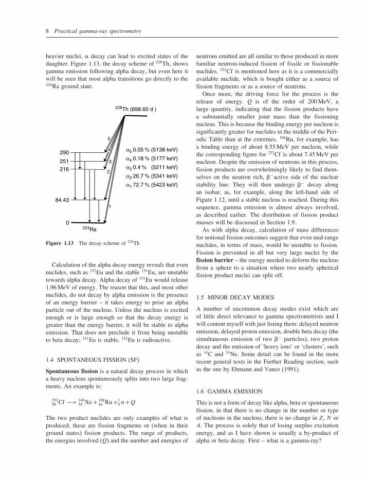
8 Practical gamma-ray spectrometry
heavier nuclei, � decay can lead to excited states of thedaughter. Figure 1.13, the decay scheme of 228Th, showsgamma emission following alpha decay, but even here itwill be seen that most alpha transitions go directly to the224Ra ground state.
0
84.43
290
251
216
228Th (698.60 d )
224Ra
1
2
3
4
5
α5 0.05 % (5138 keV)
α4 0.18 % (5177 keV)
α3 0.4 % (5211 keV)
α2 26.7 % (5341 keV)
α1 72.7 % (5423 keV)
Figure 1.13 The decay scheme of 228Th
Calculation of the alpha decay energy reveals that evennuclides, such as 152Eu and the stable 151Eu, are unstabletowards alpha decay. Alpha decay of 151Eu would release1.96 MeV of energy. The reason that this, and most othernuclides, do not decay by alpha emission is the presenceof an energy barrier – it takes energy to prise an alphaparticle out of the nucleus. Unless the nucleus is excitedenough or is large enough so that the decay energy isgreater than the energy barrier, it will be stable to alphaemission. That does not preclude it from being unstableto beta decay; 151Eu is stable, 152Eu is radioactive.
1.4 SPONTANEOUS FISSION (SF)
Spontaneous fission is a natural decay process in whicha heavy nucleus spontaneously splits into two large frag-ments. An example is:
25298 Cf −→ 140
54 Xe + 10844 Ru +1
0 n +Q
The two product nuclides are only examples of what isproduced; these are fission fragments or (when in theirground states) fission products. The range of products,the energies involved (Q) and the number and energies of
neutrons emitted are all similar to those produced in morefamiliar neutron-induced fission of fissile or fissionablenuclides. 252Cf is mentioned here as it is a commerciallyavailable nuclide, which is bought either as a source offission fragments or as a source of neutrons.
Once more, the driving force for the process is therelease of energy. Q is of the order of 200 MeV, alarge quantity, indicating that the fission products havea substantially smaller joint mass than the fissioningnucleus. This is because the binding energy per nucleon issignificantly greater for nuclides in the middle of the Peri-odic Table than at the extremes. 108Ru, for example, hasa binding energy of about 8.55 MeV per nucleon, whilethe corresponding figure for 252Cf is about 7.45 MeV pernucleon. Despite the emission of neutrons in this process,fission products are overwhelmingly likely to find them-selves on the neutron rich, �−active side of the nuclearstability line. They will then undergo �− decay alongan isobar, as, for example, along the left-hand side ofFigure 1.12, until a stable nucleus is reached. During thissequence, gamma emission is almost always involved,as described earlier. The distribution of fission productmasses will be discussed in Section 1.9.
As with alpha decay, calculation of mass differencesfor notional fission outcomes suggest that even mid-rangenuclides, in terms of mass, would be unstable to fission.Fission is prevented in all but very large nuclei by thefission barrier – the energy needed to deform the nucleusfrom a sphere to a situation where two nearly sphericalfission product nuclei can split off.
1.5 MINOR DECAY MODES
A number of uncommon decay modes exist which areof little direct relevance to gamma spectrometrists and Iwill content myself with just listing them: delayed neutronemission, delayed proton emission, double beta decay (thesimultaneous emission of two �− particles), two protondecay and the emission of ‘heavy ions’ or ‘clusters’, suchas 14C and 24Ne. Some detail can be found in the morerecent general texts in the Further Reading section, suchas the one by Ehmann and Vance (1991).
1.6 GAMMA EMISSION
This is not a form of decay like alpha, beta or spontaneousfission, in that there is no change in the number or typeof nucleons in the nucleus; there is no change in Z, N orA. The process is solely that of losing surplus excitationenergy, and as I have shown is usually a by-product ofalpha or beta decay. First – what is a gamma-ray?