practical aspects of strapdown inertial gravimetry...a few practical ideas… gravity in initial and...
TRANSCRIPT

Practical Aspects of Strapdown Inertial Gravimetry
David Becker, TU Darmstadt, Germany [email protected]

Overview
• Why Strapdown? • Kalman-Filter design • A few practical ideas… • System analysis
– Observability – Error propagation simulations
• Thermal calibration – Motivation – A simple approach – Parametric approaches (BSC, BSSC) – Sample-based approach
• Test data sets • Results
Aconcagua
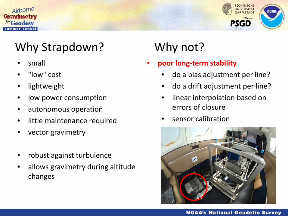
Why Strapdown? • small • "low" cost • lightweight • low power consumption • autonomous operation • little maintenance required • vector gravimetry
• robust against turbulence • allows gravimetry during altitude
changes
• poor long-term stability • do a bias adjustment per line? • do a drift adjustment per line? • linear interpolation based on
errors of closure • sensor calibration
Why not?

Overview
• Why Strapdown? • Kalman-Filter design • A few practical ideas… • System analysis
– Observability – Error propagation simulations
• Thermal calibration – Motivation – A simple approach – Parametric approaches (BSC, BSSC) – Sample-based approach
• Test data sets • Results
Aconcagua

Kalman-Filter design ("P-approach")
• 3D position • 3D velocity • 3D attitude • 3D accelerometer bias • 3D gyro bias • 3D gravity disturbance • 3D leverarm (opt.)
Observation model:
State transition model:
RC+RW RC
RC+RW 1st order GM
3rd order GM
System State:
Kalman Smoother
?
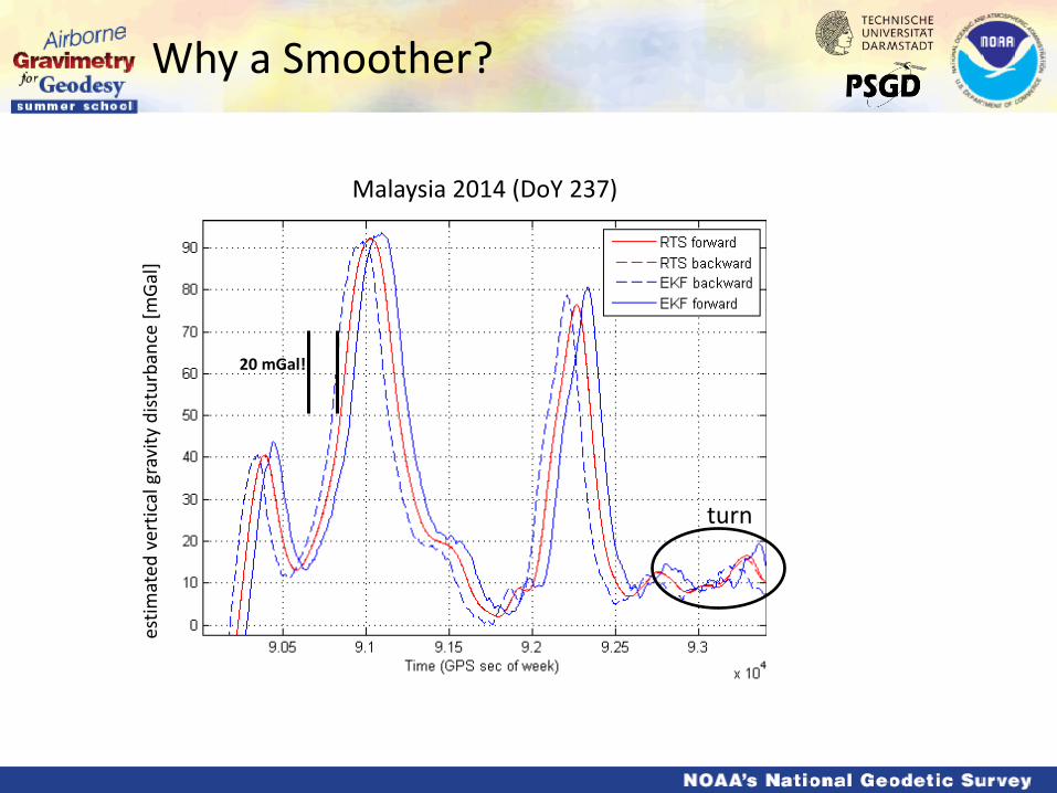
Why a Smoother?
Malaysia 2014 (DoY 237) es
timat
ed v
ertic
al g
ravi
ty d
istur
banc
e [m
Gal
]
turn
20 mGal!

A few practical ideas… gravity in initial and final aircraft position is usually known – it may be introduced as an observation here!
rate of gravity change is related to position change, not time…
ZUPT? Aircraft is shaking in parking positions, so v≠0!
GNSS antenna position is not really "static" in parking position!
If lever arm is not perfectly known, do not introduce it as such!
to enable the removal of a linear drift, the IMU must be running from start to end
Thermal drifts of accelerometers and FOG avoid temperature changes during the flight!
Let the device warm for > 5 hours before the flight, if possible.
Internal IMU clocks are drifting! Precise time stamps are crucial (few msec). Clock drifts can also be temperature dependent!

Overview
• Why Strapdown? • Kalman-Filter design • A few practical ideas… • System analysis
– Observability – Error propagation simulations
• Thermal calibration – Motivation – A simple approach – Parametric approaches (BSC, BSSC) – Sample-based approach
• Test data sets • Results
Aconcagua
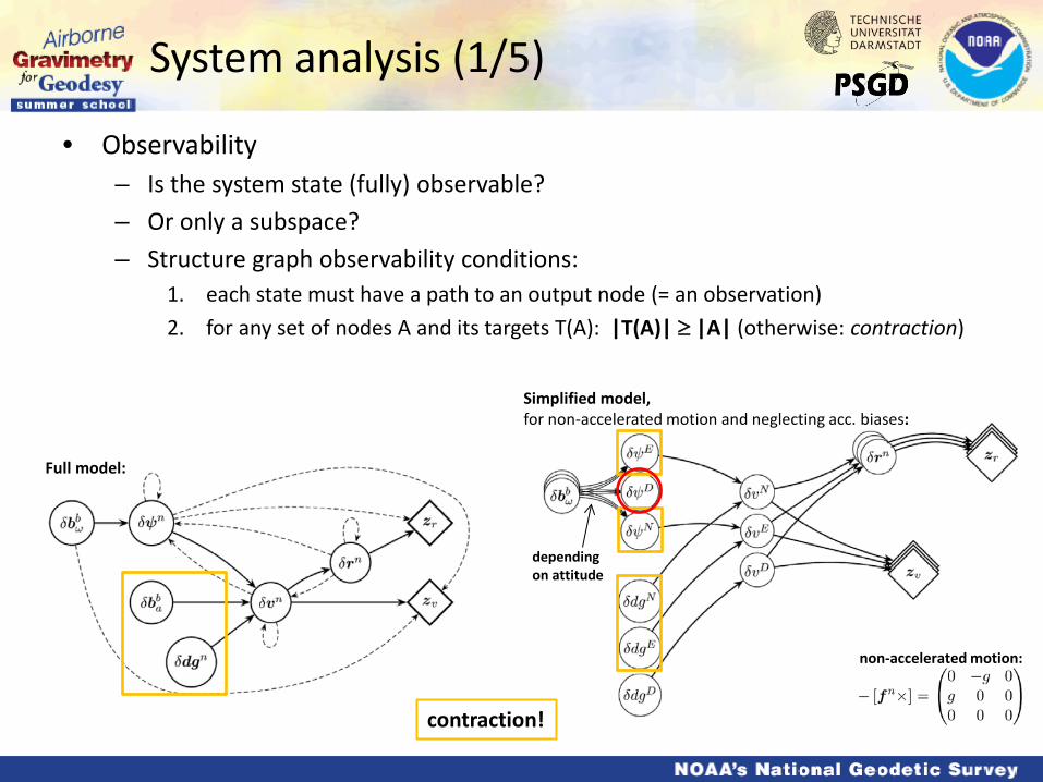
System analysis (1/5)
• Observability – Is the system state (fully) observable? – Or only a subspace? – Structure graph observability conditions:
1. each state must have a path to an output node (= an observation) 2. for any set of nodes A and its targets T(A): |T(A)| ≥ |A| (otherwise: contraction)
Full model:
Simplified model, for non-accelerated motion and neglecting acc. biases:
depending on attitude
contraction!
non-accelerated motion:

• Observability (2): algebraic definition
• coordinate and velocity observations • evaluated for different sets of active states • 4 basic scenarios for an aerogravity flight:
System analysis (2/5)
scenario w/ attitude changes
w/ horizontal accelerations
S1 S2 S3 S4

• 12 flights • 13,000 km (9,600 km on lines) • 41 h airborne (31 h on lines) • average speed: 87 m/s • used as basis for ground-truth simulation
– spline-"imitation" of attitude and velocity – spline-"imitation" of EGM gravity disturbance – exact determination of sensor measurements realistic flight characteristics
System analysis (3/5)
Simulation-based error propagation analysis
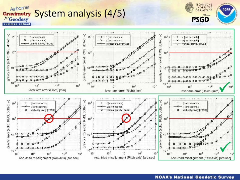
System analysis (4/5)

System analysis (5/5)
• Accelerometer bias changes on the lines are (almost) undetectable – more precisely: Gravity changes and accelerometer bias changes are almost inseparable
• A reduction of in-flight accelerometer bias changes is desirable • Calibrations may help to reduce such changes
Vertical lever arm oscillation:
Constant Z-accelerometer bias: Correlated Z-accelerometer Gaussian noise:
()

Overview
• Why Strapdown? • Kalman-Filter design • A few practical ideas… • System analysis
– Observability – Error propagation simulations
• Thermal calibration – Motivation – A simple approach – Parametric approaches (BSC, BSSC) – Sample-based approach
• Test data sets • Results
Aconcagua
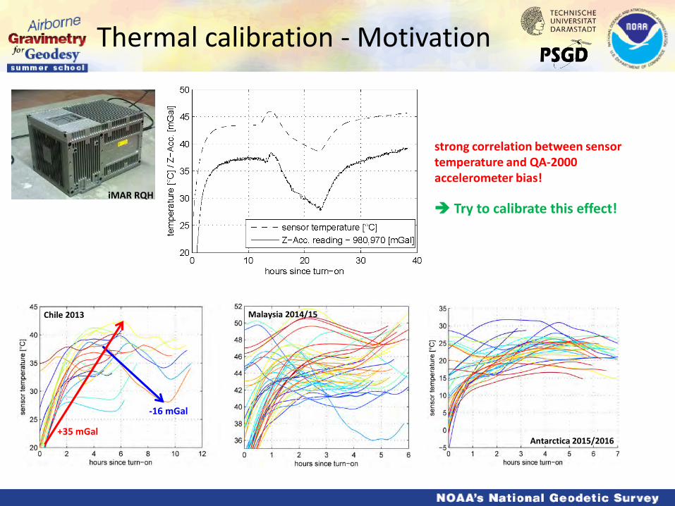
Thermal calibration - Motivation
iMAR RQH
strong correlation between sensor temperature and QA-2000 accelerometer bias! Try to calibrate this effect!
Antarctica 2015/2016
Chile 2013
-16 mGal
+35 mGal
Malaysia 2014/15

Thermal Calibration: A Simple Approach
1 2
3 4
shift to an arbitrary zero-level
compute a smoothing spline or a regresion polynomial (here: degree 4)…
… and use it as a correction for aerogravity data (with negative sign)
low-pass filtering of sensor readings

BSC-calibration
• Calibration of bias, scale factor and cross-coupling 1)
– least squares estimate with 3x3 parameters – based only on scalar observations of gravity
• requires…
– IMU at rest in different poses (e.g. face/edge/corner down 26 poses) – ground-truth scalar gravity
• Advantage: the exact orientation is not required! Can be done in the field!
1) Shin, Eun-Hwan, and Naser El-Sheimy. "A new calibration method for strapdown inertial navigation systems." Zeitschrift für Vermessungswesen.–2002.–Zfv 127.1 (2002): 41-50.
QA-2000 (in field)
bias X / Y / Z [mGal]
scale fact. X / Y / Z [ppm]
cross coupling θYZ / θZX / θZY [arcsec]
run #1 -1.6 / -2.4 / -6.5 22.5 / 19.5 / 18.8 0.1 / -3.4 / -0.4
run #2 -2.3 / 0.0 / -6.9 20.3 / 19.3 / 22.9 0.9 / -3.5 / -0.1
mean (σ) -2.0 / -1.2 / -6.7 (1.0) 21.4 / 19.4 / 20.8 (1.9) 0.5 / -3.4 / -0.3 (0.37)

Thermal BSC-calibration (1/2)
• Repeat this calibration at different sensor temperatures…
26 poses
4 oven temperatures: 10°C, 20°C, 30°C, 40°C
3 repetitions for each temperature (to check the repeatability)
1 minute per pose
sensor temperature has to be constant for each set add 3 hours waiting time after temperature change
total: ~ 19 hours (incl. table motion times)
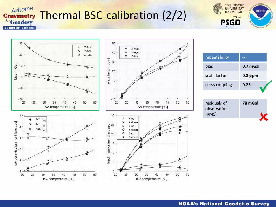
Thermal BSC-calibration (2/2)
repeatability σ
bias 0.7 mGal
scale factor 0.8 ppm
cross coupling 0.25" residuals of observations (RMS)
78 mGal

Thermal BSSC-calibration (1/2) BS
C BS
SC
Idea: Extend the error model by an additional scale factor (for negative sensor readings)
BSSC
BSC

Thermal BSSC-calibration (2/2)
Discussion • bias + scale factor or bias + 2 x scale factor are both
unsatisfactory error models! – cross-coupling might change among different poses – the good repeatability suggests that we can do better…
• so? add even more parameters to the model?
repeatability σ
bias 1.4 mGal
pos. scale factor 2.4 ppm
neg. scale factor 2.2 ppm
cross coupling 0.25" residuals of observations (RMS)
35 mGal (BSC: 78 mGal)
Comparison BSC/BSSC

Sample-based calibration (1/5)
• Idea: build a look-up table of sensor errors
1. select a sample space 2. define a set of samples to be included in the table 3. for each sample: measure the error (measured quantity – true quantity)
• masks all influences in a single value (per sensor) • error is 3-D for a sensor triad
4. if required, smooth the sample data 5. use interpolation to get correction (=neg. error) for any coordinate in
sample space

Sample-based calibration (2/5)
1. select a sample space • reasonable dimensions are
– temperature (T) (strong dependencies for accelerometers, should always be included!) – sensor reading (S) – roll angle (R) – pitch angle (P)
T (1-D) used for "simple approach"
TRPS (4-D) difficult/impossible to calibrate
TRP (3-D) vehicle accelerations unmodelled
TS (2-D) …still no (explicit) attitude modeling…
TPS (3-D) …if error is independent of roll angle
TRS (3-D) …if error is independent of pitch angle

2. define a set of samples • choose a set of relevant samples (reduce calibration time) • fixed-wing airborne gravimetry:
– ambient temperatures: -15°C…40°C (equiv. sensor temperature: -1°C…52°C) – roll: max. -45°...45° (on the lines: -5°…5°) – pitch: max: -15°…15° (on the lines: 0°…5°)
15 temperatures, 114 poses
TRP (3-D)
Malaysia 2014 (on lines)
Malaysia 2014
Sample-based calibration (3/5)

3. measure the errors • overall calibration duration: 64 hours • with a 2-DOF table, heading changes can not be
avoided to set up roll/pitch angles • deflections of the vertical may distort the calibration • estimate deflections
– additional horizontal poses – adjustment with deflections and biases as parameters
Sample-based calibration (4/5)
TRP (3-D)

4. / 5. smooth / interpolate • interpolate to regular grid in TRP-space • apply e.g. a 3-D Gaussian low-pass filter
– sensor noise may depend on temperature! – horizontally aligned accelerometers are sensitive
to small random bends (1" 4 mGal)
Sample-based calibration (5/5)
TRP (3-D)
Example: Z-accelerometer errors [mGal] (no smoothing):
0°C 30°C 50°C
mGal

iMAR RQH: Allan standard deviation
68 µGal @2500 s
0.7 mGal @100 s
Overview
• Why Strapdown? • Kalman-Filter design • A few practical ideas… • System analysis
– Observability – Error propagation simulations
• Thermal calibration – Motivation – A simple approach – Parametric approaches (BSC, BSSC) – Sample-based approach
• Test data sets • Results
Aconcagua

Test data sets (1/4): Chile 2013
• 24 flights • 88 flightlines • 30,000 km / 80 h • ~200 kts • 3,300 – 16,000 ft • 20 km line spacing

Test data sets (2/4): Malaysia 2014/2015
• 46 flights • 181 flightlines • 34,800 km, 110 h • 170 kts • 3,000-8,000 ft (mostly 6,000 ft) • 5 / 10 km line spacing
105° E 110° E 115° E 120° E 125° 0°
5° N
10° N
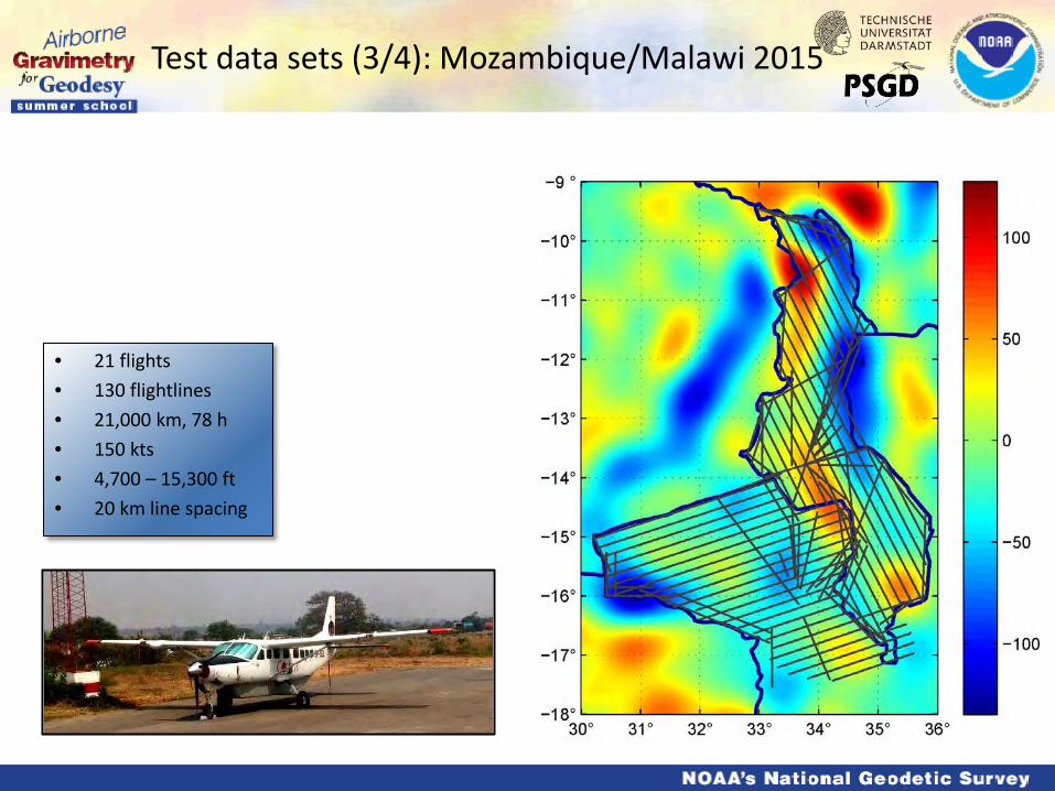
Test data sets (3/4): Mozambique/Malawi 2015
• 21 flights • 130 flightlines • 21,000 km, 78 h • 150 kts • 4,700 – 15,300 ft • 20 km line spacing

Test data sets (4/4): Antarctica Polar Gap
• 32 flights • 121 flightlines • 32,400 km, 78 h • 130 kts • 1.5 – 4.3 km

X-over RMS (σ) [mGal] Δh < 100 m
without calibration
simple Z-acc. calibration
BSC BSSC TRP
Chile 2013 (*) 6.8 (4.8) 1.75 (1.24) 1.79 (1.27) 1.89 (1.34) 1.81 (1.28)
Malaysia 2014 3.7 (2.6) 1.44 (1.02) 1.98 (1.40) 1.91 (1.35) 1.18 (0.83)
Malaysia 2015 (33 out of 34 flights)
3.5 (2.5) 1.68 (1.19) 1.82 (1.29) 1.74 (1.23) 1.71 (1.21)
Mozambique/Malawi 2015 (*) (18 out of 21 flights)
4.1 (2.9) 1.63 (1.16) 1.65 (1.17) 1.57 (1.11) 1.37 (0.97)
Antarctica PolarGap 2015/2016
4.5 (3.2) 3.2 (2.3) - - 2.9 (2.1)
Results: Thermal Calibrations (1/2)
(*) 15" topographic reductions applied in the EKF (30' RTM)
Malaysia 2014

Results: Thermal Calibrations (2/2)
Chile 2013 Errors of Closure with/without STC of Z-accelerometer

Results: Resolution RQH vs. LCR
Chile 2013 (DoY 288) LCR, IMU
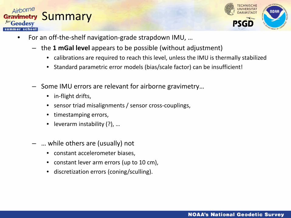
Summary • For an off-the-shelf navigation-grade strapdown IMU, …
– the 1 mGal level appears to be possible (without adjustment) • calibrations are required to reach this level, unless the IMU is thermally stabilized • Standard parametric error models (bias/scale factor) can be insufficient!
– Some IMU errors are relevant for airborne gravimetry… • in-flight drifts, • sensor triad misalignments / sensor cross-couplings, • timestamping errors, • leverarm instability (?), …
– … while others are (usually) not • constant accelerometer biases, • constant lever arm errors (up to 10 cm), • discretization errors (coning/sculling).

Outlook
A good prospect for strapdown gravimetry!
Strapdown gravimetry on miniature drones? (new RQH housing: 7.5 kg)
Getting 1 mGal from a combination of tactical-grade strapdown IMU (2-3 kg) and GGM?
Thermal stabilisation for fixed-wing aerogravity. Higher power/space/price.
Enabling a reliable 1 mGal-accuracy
iMAR RQH

Questions?
Acknowledgements
The Chile aerogravity campaign was carried out in cooperation with the Instituto Geográfico Militar, Chile, and the US National Geospatial-Intelligence Agency (NGA).
The Malaysia aerogravity campaigns were financed by the Department of Survey and Mapping Malaysia (JUPEM).
The Mozambique/Malawi aerogravity campaign was financed by NGA.