powerful goodness-of-fit and multi-sample tests by · powerful'goodness-of-fit and...
TRANSCRIPT

Powerful Goodness-of-Fit and Multi-Sample Tests
BY
Jin Zhang
A thesis submitted to the Faculty of Graduate Studies in
partial fulfillment of the requirements
for the degree of
Doctor of Philosophy
Graduate Programme in Statistics
York University
Toronto, Ontario
July 2001

National Library 1*1 ofCanada Bibliothèque nationale du Canada
Acquisitions and Acquisitions et Bibliographie Services services bibliographiques 395 WeUimgîon Street 395. rue WeUington OttawaON KlAON4 OrtawaON K i A û N 4 Canada Canada
The author has granted a non- exclusive licence allowing the National Library of Canada to reproduce, loan, distribute or seil copies of this thesis in microform, paper or electronic formats.
The author retains ownership of the copyright in this thesis. Neither the thesis nor substantial extracts fiom it may be pniited or otherwise reproduced without the author's permission.
L'auteur a accordé une licence non exclusive permettant à la Bibliothèque nationale du Canada de reproduire, prêter, distribuer ou vendre des copies de cette thèse sous la forme de microfiche/film, de reproduction sur papier ou sur format électronique.
L'auteur conserve la propriété du droit d'auteur qui protège cette thèse. Ni la thèse ni des extraits substantiels de celle-ci ne doivent être imprimés ou autrement reproduits sans son autorisation.

Powerful'Goodness-of-Fit and Multi-Sample Tests
by Jin Zhang
a dissertation submitted to the Faculty of Graduate Studies of York University in partial fuLfillment of the requrements for the degree of
DOCTOR OF PHILOSOPHY
Permission has been granted to the LIBRARY OF YORK UNIVERSIW to lend or seil copies of this dissertation, to the NATIONAL LIBRARY OF CANADA to microfilm ths dissertation and to lend or seU copies of the film, and to UNlVERSrrY MICROFILMS to publish an abstract of this dissemition. The author reserves other publication rights. and neither the dissertation nor e-xtensive extracts from it may be printed or otherwise reproduced without the author's wxitten permission.

Abstract
There are a large numkr of goodness-of-fit tests in the literature. The
most cornmon used tests are Pearson's chi-squared tests and EDF
(empirical distribution function) tests. such as Kolmogorov-Srnirnov,
Cramer-von Mises and Anderson-Darling tests. The chi-squared tests are
easy to use, but they are generally less powerful than EDF tests.
A parameterization approach is proposed to construct a generai goodness-
of-fit test for a specified distribution Fo. It includes traditionai EDF tests,
as well as new likelihood-ratio tests, which are the analogues of the old
tests in representation but are generally much more powerful.
If Fo has some unknown parameters. we need to estimate the parameters
first and then apply the tests. Thus, we can test the goodness of fit for a
family of distributions. To test normality, for example, suppose Fo is a
normal distribution with unknown mean and variance, we can estimate
them by the sample mean and variance. Then the new tests can be applied
to test the goodness of fit for normality. In such a case, they outperform
the best tests of normaIity in the Iiteranire according to Our simulation.

The rnethodolcigy developed for goodness-of-fit tests is applied to the
general two-sarnpIe problems. Similarly, we can not only generate
classical two-sarnple tests, but also produce new powerfil tests, which are
sensitive to the difference in location, scde and shape between the
distributions of the two-sampled populations. Conventional tests, however,
are location-sensitive only.
Besides, the new two-sample tests are generdized to multi-sample tests,
and parailel results have been obtained.
Since the exact sampling distributions of the EDF test statistics are
intractable, a simple distribution family is introduced to approximate their
sampling distributions in the end,
Acknowledgments
1 take this opportunity to express my sincerest gratitude to Professor
Yuehua Wu, my supervisor for PhD. thesis- I have benefited greatly from
her for academic guidance, financial support and ail kinds of helps, which
led to my successful Ph.D. study at York University. From the bottom of
my heart, 1 thank her for her kindness and friendship. 1 also thank
Professors Georges Monette and Jianhong Wu, two other members of the
Supervisory Committee, for their precious suggestions and helps.
1 am grateful to my teachers for their kindly help and encouragement,
especiall y to Professors Stephen Chamberlin, Peter Song and Masoud
Asgharian, whom 1 had good fortune to learn from. My thanks are
extended to the facuIty and staff at the Department of Mathematics and
Statistics, York University.
I would like to thank the Department of Mathematics & Statistics and the
Faculty of Graduate Studies of York University, for the financial support
of George and Frances Denzel Award for Excellence in Statistics and the
Dean's Academic Excellence Scholarships,
Finally, 1 am indebted tremendously to my wife Jikun Yi and our daughter
Yili Zhang, who sacrificed much and supported me to complete my P h D .
study.
Table of Contents
Abstract
Acknowledgments
List of Tables
List of Illustrations
1. Introduction
2. Traditional Goodness-of-Fit Tests Based on EDF
3. New Powerful EDF Tests
4. Power Comparison by Simulation
5. The Distributions of ZA, and ZK
6. Tests of Norrnality
7. Comparison of Power for Testing Nonnality
8. General Two-Sample Problem
9. New PowerfuI Two-Sample Tests
10. Power Cornparison for Two-SampIe Tests
1 1. The Distributions of Two-Sarnple ZA, & and ZK
12. General k-Sample Problem
13. New k-Sarnple Tests
14. Power Comparison for k-Sample Tests
15. The Distributions of k-Sarnple ZAY and ZK
16. Beta Approximation to the Distribution of Ks
17. A Simple Distribution Family
18. Approximate distribction for Crarnér-von Mises Statistic
19. Approximate Results for Waston's Statistic
20. Concluding Remarks
References
vi i

List of Tables
Table 5.1. Percentage points for 1 OZA-32
Table 5.2. Percentage points for Zc
Table 5.3. Percentage points for ZK
Table 6.1. Percentage points for ZA when testing normality
Table 6.2. Percentage points for Zc when testing normality
Table 6.3. Percentage points for ZK when testing normaiity
Table1 1.1. Times to Breakdown of an Insulating Fluid
Table 16.1 .The moments of Ks and aBPq+b
Table 16.2.The moments of Ks and corresponding a, b, p, q
Table 16.3. Percentage points for Ks
Table 18.1. Some values of a, b, p, q
Table 18.2. Some percentage points for w2
Table 19.1. Some values of a, b, p, q
Table 19.2. Some percentage points for U*
viii

List of IiIustrations
One-Sarnple Tests
Fig. 4.1. Powers for testing U(0, 1) vs Beta(p, q)
Fig. 4.2. Powers for testing N(p, a2) vs t(k) or Gamma(r, 1)
Fig. 4.3. Powers for testing N(0, 1) vs N(p, 02)
Fig. 7.1. Powers for testing Normal vs Beta(p, q)
Fig. 7.2. Powers for testing Normal vs t(k) or Garnma(r, 1)
Fig. 7.3. Powers for testing Normal vs Weibull or Lognormal
Two-Sarnple Tests
Fig. 10.1. Powers for testing U(0, 1) vs Beta(p, q)
Fig. 10.2. Powers for testing N(0, 1) vs N(p, 02)
Fig. 10.3. Powers for testing N(p7 c2) vs Gamma@, 1)
k-SampIe Tests
Fig. 14.1. Powers for testing U(0, 1) vs Betafpi, qi) (i=2,3)
Fig. 14.2. Powers for testing N(0, 1) vs N(& , ai2) (i=2,3)
Fig. 14.3. Powers for testing N(p, 2) vs Gamma(ai, bi) (i=2,3)
Fig. 14.4. Powers for testing N(0.5,O. 1) vs Beta(pi, qi) (i=2,3)

To rny mother Zhenying Zhu,
my wife Jikun Yi,
and Our daughter Yili Zhang
In the memory of my father Junmo Zhang

1. Introduction
There are many kinds of goodnessof-fit tests in the literature. Some of them
are special purpose tests, so that they are suitable and perform well only for sorne
special situations. Others are omnibus tests that are applicable to general cases.
The most common used omnibus tests are Pearson's chi-squared tests and the
tests based on EDF (empirical distribution function), such as traditional Kolmogorov-
Smirnov, Cramer-von Mises and Anderson-Darling tests. Chi-square tests are easy
to use, but they are generally less powerful than EDF tests (DIAgostino and Stephens,
1986).
We now introduce a new method based on parameterkation, which c m not only
generate traditional EDF tests, but also produce new powerful omnibus tests.
Let X be a continuous random variable with distribution function F ( x ) , and XI,
-Y2, ...? .Y, be a random sample from X with order statistics X(l), X p ) , --., X(*)-
We wish to test the nui1 hypothesis
H : F ( x ) = &(x),
against the general alternative
ti- : F ( x ) # Fo(x),
for al1 x E (-00, oo)
for some x E (-CO, m)
where Fo(x) is a hypothesized distribution function to be tested. Here we discuss
only the basic situation where Fo(z) is completely known. For other cases, see

Section 6 . Note that
with Ht : F ( t ) = Fo(t) and Ht : F ( t ) # Fo(t). Then testing H vs. H is equival ent
to testing Ht vs. Rt for every t E (-XI, m).
To test Ht vs. with t fixed, we have a binary random sample based on the
indicator function: ,Y,t = I ( X ï 5 t ) (i = 1,2, ..., n) satisfying P(X*t = 1) = F( t )
and P ( S i t = 0) = 1 - F(t) .
Note that F ( x ) is an unknonm distribution function arbitrary, while F ( t ) with
t fked is nothing but a unknown parameter. Through introducing the new binary
sample, the nonparametric test for H vs. H is simplified to a family of parametric
tests for Ht vs. H ~ , t E (-ca, oo). The simplification is a process of parame-
terization, through which parametric approaches can be applied to nonparametric
tests.
For each fixed t E (-cm, w) and the corresponding random sample Xit, X2t, .-., Xnt,
let Zt be a statistic for testing Ht vs. H~ such that its large values reject Ht. Then
two types of statistics for testing H vs. H can be defined by
00
= /__ zt and Z,, = SUP [ Ztw(t) ] , t€(-w, oc)
(1-1)
where w( t ) is sorne weight function and large values of Z or Z,, reject the nul1
hypothesis W.
The power of Z or Z,, depends on Zt and w(t) . Two natural candidates for Zt
are Pearson's chi-squared test statistic and the Iikelihood-ratio test statistic, which

are respectively (after simplification)
n[Fn(t) - FWI2 X' = Fo (t) [i - FO (t)]
and
where F'(t) is the empirical distribution function of the original sample XI, X2, ...,
A large family of Zt which embeds X: and G: can be obtained by using the
Cressie and Read (1984) family of divergence statistics 2nIA for testing the good-
ness of fit of a multinomial distribution. In fact, for the above binary sample
X l t , ..., Xnt with t fixed, the Cressie-Read farnily of divergence statistics
for testing Ht vs. H t is
which includes Xf ( X = l ) and G: (X=O), as well as other important statistics (Cressie
and Read 1984; Read and Cressie 1988).
We focus on X: and G: because X: is associated with classical tests while G: is
the best choice of Zt in (1.1) among the family (1.4) according to our simulation.
By choosing different weight functions, we \vil1 show in Sections 2-4 by simulation
that (a) using X: as Zt generates traditional EDF test statistics; (b) using G: as Zt
produces new EDF tests; (c) the new EDF tests are generally more powerful than
traditional goodness-of-fi t tests.
The sampling distributions of the new test statistics are intractable. Their em-

pirical percentage points are given in Section 5. In Sections 6-7, we will consider
the case when Fo has some parameters unknown. As a typical example, we discuss
the goodness-of-fit test for normality, which is a fundamental issue in statistics and
has always been a hot topic in the literature. Our simulation indicates that the new
EDF tests outperform the best tests of normality in the literature.
In Sections 9-11, the idea of parameterization for one-sample tests is developed
and applied to the general two-sample problem. Similarly, we can not only generate
traditional two-sample tests, but also produce new powerful distribution-free tests.
Furthermore, the results for two-sample tests are generalized to k-sample tests (see
Sections 12-15). Monte Carlo simulation shows that conventional multi-sample tests
are sensitive to location difference among distributions, but are du11 to detect the
variation in shape. However, the new tests are both location- and shape-sensitive.
-4 simple distribution family is introduced in Section 16-19 to approximate the
distribution functions of goodnessof-fit test statistics, but the approach is applicable
to general continuous random variables. Some traditional EDF test statistics are
used as illustrative examples. Finally, concluding remarks are given in Section 20.
2. Traditional Goodness-of-Fit Tests Based on EDF
Using X: in (1.2) as Zt in (1.1) but choosing different weight functions, we can
derive traditional goodness-of-fit tests based on EDF. Below are three examples.

Replacing Zr of statistic Z,, in (1.1) with X: in (1.2) generates
where Ks is the Kolmogorov-Smirnov statistic, the most well-known statistic for
goodness-of-fit tests (Kolmogorov, 1933; Smirnov, 1939; Massey, 1951; Stephens,
1970, 1974; Conover, 1980; Pratt and Gibbons, 1981; D'Agostino and Stephens,
1986; Gibbons, 1992; Cabana, 1996).
Replacing Zt of statistic Z in (1.1) with X: in (1.2) generates the Anderson-
Darling statistic
2 " = - - [(i - 0 . 5 ) 1 0 g F ~ ( X ( ~ ) ) + (n - i + 0-5)log[l - ~o(x(i,)]] - n , i = l
one of the most powerful and important goodness-of-fit tests in the literature (An-
derson and Darling, 1952, 1954; Stephens, 1970, 1974; D'Agostino and Stephens,
1986; Sinclair and Spurr, 1988). The last equality here (as well as that below) can
be obtained by evaiuating the associated integral.
Replacing Zt of statistic Z in (1.1) with X: in (1.2) generates the famous Cramér-
von Mises statistic (Crarnér, 1928; von Mises, 1931; Smirnov, 1936, 1937; Stephens,
1970, 1974; Knott, 1974; Conover, 1980; D'Agostino and Stephens, 1986; Csorg6

and Faraway: 1996; Spinelli and Stephens, 1997)
3. New Powerful EDF Tests
As a goodness-of-fit test for a multinomial distribution, the Pearson's chi-squared
statistic is asymptotically equivalent to the li kelihood-ratio statistic. Therefore,
under the nul1 hypothesis Ht in Section 1, the chi-squared statistic Xf in (1.2) and
the likelihood- ratio statistic G: in (1.3) are equivalent in large sample situations,
but they are different under the alternative H ~ . We have seen in Section 2 that
traditional tests can be generated by using X: as Zt in (1.1). In this section we
shall use G: to produce new powerful tests by choosing proper weight functions.
For any continuous hypothetical distribution function Fo, let U, = Fo(Xi) (2-1,
2, ..., n) so that U(,) = Fo(X(i))- Note that XI, X2, .--, Xn are i.i.d. from Fo if and
only if Ui, U;, ..., Un are i.i.d. from U(0, l), the standard uniform distribution. To
test H vs. H, consider a statistic with form T = T(U1, Li2, . Un) , where T(- . -) is
a given function independent of Fo. Since U, and 1 - Ui are identically distributed
under Hl a reasonable T should satisfy
In such a case, we say that T is distribution-symrnetric about the median.
It is obvious that the traditional statistics Ks, IV2 and A2 in Section 2 are

functions of Ul, U2, ..-, Un, and they are distribution-symmetric. In order to gen-
erate new distribution-symmetric tests, we have to choose proper weight functions.
Moreover, we sometimes need to make modifications to Fn(t) at its discontinuous
points X(i) (i = 1 , 2, ..., n) by defining Fn(X(i)) = (i - c ) / ( n + l - 2c), where c
is a constant between O and 1. The natural and intuitive choice of c is 0-5 so that
Fn(X(q) = (i - 0.5)ln or [Fn(X(i) - 0) + Fn(X(il + 0 ) ] / 2 , which is a common way
(something like continuity correction) to modifi the empirical distribution function.
In fact, we can imagine that at point x = X(i), there are i - 0.5 or n - i + 0.5
observations among XI, X2, ..., X, which are less or greater than the x. Indeed,
our simulation shows that c = 0.5 seems to be the best choice in terms of power.
Finally, the traditional test statistics in Section 2 also suggest that Fn(X(i)) should
be (i - 0.5)/n instead of i/n.
When necessary, we always define F, ( X ( i ) ) = (i - 0-5)ln. Then new distri bu tion-
symmetrïc tests can be generated by choosing proper weight functions as follows.
Let X(o) = -00 and X(n+l) = m. Replacing Zt of statistic Z,, in (1.1) with
G: in (1 -3) produces
sup G: = max { sup G: } = m+x G ~ X ( ~ , , t€ ( -00 , w) O.liSn X ( i ) ~ t < X ( i + l ) l<rsn
which is equivalent to

Replacing Zt of statistic Z in (1.1) with G: in (1.3) produces
which is equivalent to
Replacing Zt of statistic Z in (1.1) with G: in (1.3) produces
where C, is a constant and bi = i l o g ( i / n ) + (n - i ) l o g ( l - i /n).
Since bi-l - bi = l o g [ ( n - 0 .5 ) / ( i - 0.75) - 11, the above test statistic is approx-
imately equivalent to
The new statistics ZK, Za and Zc are distribution-symmetric. They look like
traditional Ks, A* and CV2 respectively, but they are generally much more powerful.
According to Our simuiation, they are sensitive not only to the location or scale, but
also to the shape of the alternative distribution.
4. Power Cornparison by Simulation
In this section we will use the Monte Car10 approach to simulate the powers
of the new statistics ZA, Zc, ZK and the traditional I~olrnogorov-Smirnov statistic

Ks, Cramér-von Mises statistic W 2 , Anderson-Darling statistic A2 and Pearson's
chi-squared statistic X2. For the chi-squared test, the sample observations need be
grouped. Here we use the associated functioa in Splus with default values (See,
e.g., S-PIUS 2000 Guide to Statistics, Volume 1, Data Analysis Products Division,
MathSoft, Seattle, WA, p. 100).
The simulation size is 10,000, and the significance 1weI or the probability of type
1 error for testing goodness of fit is a = 0.05. For various situations about the null
hypothesis H and the alternative H, dl simulated powers for the seven statistics
are illustrated with graphs, where the powers are plotted against the sample size n
for selected values of n=10, 20, 30, 50, 70, 100, 150, 200 and 300.
E x a m p l e 4.1:
lid H : X , . X U(0 , 1) us. H : X I , ..., X,, Beta(p , q)
Without loss of generality, ive can assume that the underlying distribution F
is the standard uniform U(0, 1) under the null hypothesis H. Then the natural
candidate for F under the alternative A is the beta distribution Beta(p, q) with
parameters p and q , which includes the uniform U(0, 1) or Beta(1, 1). So, this
esarnple is actually a parametric test for H : , q) = (1, 1) us. H : (p, q) # (1, 1).
For (p, q) = (0.6, O.8), (0.6, 0.6), (0.8, 0.8), (1.3, 1.3), (1.6, 1.6), (1.3, 1.6), the
powers of Zs4, Zc, ZK, Ks, IV2, A2, X2 under A are plotted in Fig. 4.1 respectively.
WC see that ZA or Zc fias the highest power in the cases where pl q > 1 or pl q < 1 ,
and they dorninate al1 others. Although ZK is not as powerful as ZA and Zc, it is
still overwhelmingly pomerful compared to its analogue Ks.

We also consider the power of the entropy-based test of uniformity proposed by
Dudewicz and van der Meulen (1981). Their method involves choosing the best
integer m which depends on the sarnple size n, but their power results in Table 3 are
obtained from choosing the best m not only for different n but also for different alter-
native distributions. Of course, different tests fit different models. However, when
performing a nonparametric test, we have no idea about the alternative distribution.
Therefore, if a fked m is used for the same n but different alternative distributions,
the power of such a test is generally lower than that of Anderson-Darling test A*.
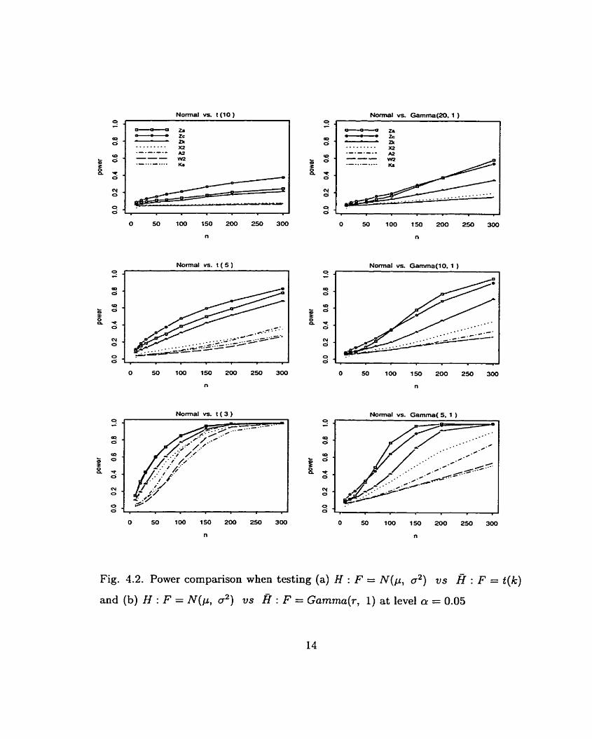
iid H : Xi, ..., X, hl N ( p , cr2) US- H : Xi, -.., X,, %! t ( k )
Because of the importance of the normal distribution, F is âssumed to be a
normal distribution N ( p , 02) under the nul1 hypothesis H. It is interesting to
consider that (a) F also has a symmetric distribution under the alternative H , say
t ( k ) , the t distribution with k degrees of freedom; (b) both distributions have the
same mean and variance, i.e. p = O and o2 = k/(k - 2).
Since N(0 , 1) = t(oo), testing H : F = N ( p , a*) us. H : F = t ( k ) is
equivalent to testing H : k = co us. H : k # W. Fig. 4.2 compares the powers
of the seven statistics &, ZC, ZK, Ks, IV2, A2, X2 for k=3, 5, 10. Obviously Zc
is the best and ZA? Zc, ZK dominate the others (sometimes they are rnuch more
powerful) .
The Cauchy and logistic distributions are also typical examples of symmetnc
distributions, which can be considered as the underlying distribution under H. The

pourer cornparison for logistic distribution is just like that for t ( 9 ) , while the Cauchy
distribution is t (1 ) .
In this example F is also assumed to be N ( p , 02) under H, but it has an
asymmetric distribution under H , such as Gamma(r, l ) , the gamma distribution
with shape parameter r and scale parameter 1, which includes exponential and chi-
squared distributions. We also assume that both distributions have the same mean
and variance, i.e. p = r and o2 = T .
Similarly, since the asymptotic distribution of Gamma(r, 1) is normal when
r + oo, testing H : F = N ( p , 02) US. H : F = Gamma(r, 1) is equivalent to
testing H : r = w us. H : r # W.
Simulated powers of the seven statistics for r=5, 10 and 20 are also plotted in
Fig. 4.2, which shows that (a) ZA, Zc, ZK dominate the others; (b) the powers of ZA
and Zc are sometimes substantially higher than those of the traditional statistics.
Other asymmetric distributions, such as the log-normal, Weibull, F and Beta
were also considered as alternative distributions against the normal. These situations
are similar t o that of gamma.
Example 4.4:

In the last example, F is assumed to be normal under both H and ff. Without
loss of generality, we need to consider only the test for H : F = N ( 0 , 1) us. H : F = N ( p , a2), or equivalently, H : (pl 02) = (0, 1) us. H : (p , 02) # (0, 1).
Six cases are considered with alternatives (1) N(0.1, l), (2) N(0.4 , l ) , (3)
N ( 0 , 1.5), (4) N(0 , 2), (5) N(0.1, 2) and (6 ) N(0.4, 1.5). Note that in cases
1 and 2, the two distributions have the same variance but different means, and in
cases 3 and 4, they have the same mean but different variances. In cases 5 and 6 ,
means and variances are both different.
For normal models, the distributions differ in mean and variance only. There
is no shape difference in terms of skewness and kurtosis. For each case Fig. 4.3
compares the powers of the seven tests, as well as the optimal parametric t- test and
the X2-test for normal mean and variance.
It is clear that for cases 1, 2, 6 where the major difference between the two dis-
tributions arises from means rather than variances, there is no signifiant difference
in poaer between the new tests and their analogues A2, CV2 and Ks. Conversely, for
the other three cases, the advantage of the new tests is obvious. When the diflerence
in distribution arises from means only, such as cases 1 and 2, the six tests are almost
as powerful as the optimal t-test. In cases 3 and 4 where the only difference cornes
from variances, the power lost by using the new tests over the x2-test is much less
than that by using their analogues. Among A', Mi2 and Ks, A2 is almost the best
in al1 cases, which is also true for other examples.

Uniform vs. Beta(O.8.0.8) Uniform vs. Beta(1 .S. 1.3)
Uniform vs. Beta(O.6.0.6)
Uniform vs. Betac0.6.0-8)
x i : I
n
Uniform vs. Beta(l.6. 1.6)
Uniforrn vs. Betafl.3. 1.61
Fig. 4.1. Power cornparison when testing H : F = U(0 , 1) us : F = Beta(p, q)
at level a! = 0.05
Normal vs. t (10 ) Normal vs. Gammat20.1 1
Normal vs. t ( 5 ) 0 1
Normal vs. 1 ( 3 )
Normal vs. Gamma(l0. 1 ) 1
n
Normal vs. Gamma( 5. 1 1
Fig. 4.2. Power cornparison when testing (a) H : F = a2) vs H : F = t ( k )
and (b) H : F = N ( p , 02) US H : F = Gamma(r, 1) at level a = 0.05

N(0. 1) vs. NCO. 1-51
N(0. 1 ) vs. N(0.4. 1.5)
O 50 100 150 200 250 300
n
Fig. 4.3. Power comparison when testing H : F = N(0 , 1) us H : F = N ( p , 02)
at level û, = 0.05

5. The Distributions of ZA, ZC and ZK
Like the Anderson-Darling A2, Cramér-von Mises W2 and Kolmogorov- Smirnov
Ks, the new statistics ZA, ZC and ZK are distribution- free. Our simulation on skew-
ness and kurtosis shows that the sampling distributions of ZA, ZC and ZK converge
very sIowly. Therefore, it is of limited practical value to study their asymptotic
distributions. Just as for A2, W2 and Ks, it is difficult to find their exact nul1
distributions for finite sample cases except for small sample sizes.
Again Monte Car10 simulation is used to approximate the percentage points of
ZA, Zc and ZK for some selected sample sizes. Tables 5.1-5.3 respectively give their
approximate percentage points, which are based on a simulation of size one million.
The pquantiles or percentage points of these tables are provided for use a t p =
0.001, 0.01, 0.05, 0.10, 0.20, 0.30, 0.40, 0.50, 0.60, 0.70, 0.80, 0.90, 0.95, 0.99, 0.999.
The simulation error in Tables 5.1-5.3 can be estimated in terms of confidence
intervals for the true percentage levels rather percentage points. For each simulated
percentage point a t level p, the 99.73% confidence interval for the true percentage
level is p f 3\ lp( l - p ) / N , where N=1,000,000 is the replicates of simulation. Thus,
the 99.73% confidence intervals for the true percentage levels in Tables 5.1-5.3 are
respectively 0.001 & 0.0001, 0.01 & 0.0003, 0.05 & 0.0007, 0.10 4z 0.0009, 0.20 &
0.0012, 0.30~0.0014, 0.4f0.0015, 0.50~0.0015, 0.60k0.0015, 0.70+0.0014, 0.80+
0.0012, 0.90 z t 0.0009, 0.95 & 0.0007, 0.99 5 0.0003, 0.999 z t 0.0001.


TABLE 5.1. (b) Percentage points for 10ZA - 32 (Upper Tail)
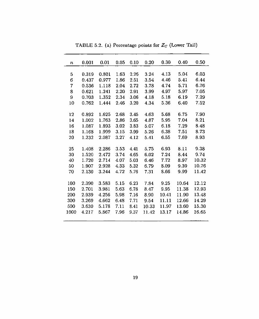
TABLE 5.2. (a) Percentage points for Zc (Lower Tail)

TABLE 5.2. (b) Percentage points for Zc (Upper Tail)

TABLE 5.3. (a) Percentage points for ZK (Lower Tail)

TABLE 5.3. (b) Percentage points for ZK (Upper Tail)

6. Tests of Normality
We discuss the goodness-of-fit tests for a specified distribution in Sections 1-
5 where the underlying distribution function Fo(x) is assumed to be completely
known. To discuss the goodness-of-fit tests for a family of distributions, Suppose
now that Fo(x) has some unknown parameters. In such a case, we need to estimate
the parameters first and then apply the test statistics ZK, ZC and Za in (3.1)-(3.3).
However, the statistics are no Ionger distribution-free because we are testing the
goodness of fit for a family of distributions instead of a specific one. For different
farnilies, the sampling distributions of the statistics are different.
Since normal distributions are the rnost important distributions in statistics, we
now consider the normal distribution farnily N ( p , 02) with mean p and variance 02.
To test if X has a normal distribution N ( p , 02) with p and 02 given, ZK, ZC and
Ze4 can be used as goodness-of-fit test statistics with Fo(x) = @(y), where 0 ( x )
denotes the distribution functiori of N(0, l), the standard normal distribution.
UsualIy, p and a > O are unknown parameters. Then tests based on ZK, Zc
and are not applicable because Fo(x) is unknown. In such a case, we estimate
p and o by the sarnple mean X = $ ZF, Xi and the sample standard deviation
s = ,/A Cy==, (,Yi - X)* respectively and then apply the goodness-of-fit tests. It is
recommended to always estimate the parameters no matter whether they are known
or not. Estirnating the parameters from the data can improve the power of the tests
when they are actually known (see the end of Section 7).
Cornparison of the powers for testing normality will be given in the next sec-

tion, where ZKr ZC and ZA are compared with the best existing test statistics,
including the Shapiro-Wilk statistic W (Shapiro and Wilk, 1965, 1968), Anderson-
Darling statistic A2 (Anderson and Darling, 1952, 1954) and D'Agostino7s statictic
D (D7Agostino, 1971, 1973).
The sarnpling distributions of ZA, ZC and ZK are intractable. Table 6.1, 6.2,
and 6.3 respectively give their approximate percentage points for testing normality,
which are based on Monte Cario simulation of size 1,000,000. The p-quantiles or
percentage points in these tables are provided for use at p = 0.001, 0.01, 0.05, 0.10,
0.20, 0.30, 0.40, 0.50, 0.60, 0.70, 0.80, 0.90, 0.95, 0.99, 0.999.
The simulation error in Tables 6.1-6.3 can be estimated in terms of confidence
intervals for the true percentage levels rather percentage points. For each simulated
percentage point a t level p, the 99.73% confidence interval for the true percentage
level is p f 3Jp( 1 - p ) / N , where N=1,000,000 is the replicates of simulation. Thus,
the 99.73% confidence intervals for the true percentage levels in Tables 5.1-5.3 are
respectively 0.001 & 0.13001, 0.01 & 0.0003, 0.05 31 0.0007, 0.10 I 0.0009, 0.20 &

TABLE 6.1. (a) Percentage points for ZA when testing normality (Lower Tail)

TABLE 6.1. (b) Percentage points for ZA when testing normality (Upper Tail)

TABLE 6.2. (a) Percentage points for Zc when testing normality (Lower Tail)

TABLE 6.2. (b) Percentage points for Zc when testing normality (Upper Tail)

TABLE 6.3. (a) Percentage points for ZK when testing normality (Lower Tail)

TABLE 6.3. (b) Percentage points for ZK when testing normality (Upper Tail)

7. Cornparison of Power for Testing Normality
There are a large number of tests for normality in the literature (e-g., D7Agostino
and Stephens, 1986) since normal distributions are the most important ones in
statistics. Sorne of these tests are only sensitive to certain kinds of departures from
norrnality, such as directional tests based on skewness and kurtosis. Thus they are
suitable and perform well only for some special situations. Others are omnibus tests,
which are applicable to general cases.
It is well known that the rnost powerful omnibus test of normality in the litera-
ture is the Shapiro-Wilk statistic W (Shapiro and Wilk, 1965, 1968; Shapiro, Wilk
and Chen, 1968), which is essentially the squared ratio of the best linear unbiased
estimator for scale to the standard deviation. Unfortunately, W is applicable to
small sarnple sizes only. In fact, FY is computable exactly up to n=SO, and valid a p
proximations exist up to n=50. Therefore, various kinds of modifications to the W
have been made, including the Shapiro and Francia's (1972) W' and the well-known
D7Agostino's (1971, 1973) statistic D which we will discuss soon, but more or less
they loose some powers (e.g., D'Agostino and Stephens, 1986).
Another important omnibus test of normality is the Anderson-Darling statistic
A2 (Anderson and Darling, 1952, 1954; Stephens, 1974; Sinclair and Spurr, 1988),
which is slightly less powerful than W but is the best existing EDF test (D'Agostino
and Stephens, 1986, p. 404).
As general goodness-of-fit tests, the new EDF statistics Zfi ZC and ZA in Section
3 are much more powerfui than traditional ones. When used as omnibus tests of

normality, they are expected to perform well. In the following, we will compare the
powers of the s k statistics ZK, ZC ZA, W , A2 and D for various kinds of situations
about alternative distributions for testing normality. Monte Carlo approach is used
with simulation size 10,000, and the significance level of the test is a = 0.05. For
each situation, the simulated powers of the six statistics for n=10, 20, 30, 40, and
50 are plotted for cornparison (the FV test requires n 5 50).
Example 7.1: Normal vs Beta(p, q)
In the first example of testing normality, the alternative distribution is the beta
distribution Beta(p, q) with parameters p and q, which is symmetnc when p = q and
includes the standard uniform distribution U(0, l)=Beta(l, 1) and an asymptoticly
normal distribution, i.e, Beta(oo, m).
The powers of ZK, ZC ZAl W, A* and D are plotted in Fig. 7.1 for (p, q)=(2,
2), (2, l ) , (1, 1.5), (1, l ) , (0.5, 1) and (0.5, 0.5), which correspond to different beta
distributions with various departures from normality.
We can see that the performance of the DIAgotino's statistic D is extremely poor
with its power almost equaling the significance level a = 0.05 for some cases. The
differences in power among Zc, ZA and W are not so obvious for al1 cases. None
of these three statistics is aIways the best, but overall, they are the best among the
six statistics. It seems that A2 generally performs a little bit better than ZK (refer
to other examples).
Example 7.2: Normal vs t ( k )

In the second example, the alternative distribution is t ( k ) , the t distribution with
k degrees of freedom, which is symmetric and includes Cauchy distribution, Le., t(1)
and the standard normal distribution N(0 , 1) = t(oo). For different values of k, the
powers of the six statistics are plotted in Fig. 7.2. In al1 cases, there is no major
difference of powers among them with D being the best and W the worst.
Example 7.3: Normal vs Gamma(a, b)
In the third exarnple, the alternative distribution is Gamma(a, b), the gamma
distribution with shape parameter a and scale parameter b, which includes exp-
nential and chi-squared distributions.
Since al1 six statistics ZK, ZC ZA, W, A* and D are invariant under any affine
transformation Y = (X - c ) / d with d > O, we need just consider Gamma(a, 1)
without loss of generality, which is a non-symmetric distribution but is asyrnptoticly
normal as a goes into infinity.
The powers of these statistics for different values of a, Say 1, 3 and 7, are also
e-xhibited in Fig. 7.2. It can be seen that ZA is the best and dominates the others.
There is almost no difference in power between Zc and W, which are slightly less
powerful than Z4. Also, there are no major differences between ZK and A*. Finally,
D behaves poorIy and is dominated by the others.
Example 7.4: Normal vs Weibull(a, b)
In the fourth example, the alternative distribution is Weibull(a, b ) , the Weibull
distribution with shape parameter a and scale parameter b.

-4s in Example 7.3, we just need t o consider Weibull(a, 1) without loss of gen-
erality. Fig. 7.3 compares the powers of the six statistics for different values of a.
The results are much similar to those in Example 7.3, but the advantage of ZA is
more obvious.
Example 7.5: Normal vs Lognormal(p, a)
In the last example, the alternative distribution is Lognormal(p, O) , the lognor-
mal distribution with pararneters p and o. We just consider the case of Lognormal(0, o)
since it has the same skewness and kurtosis as Lognormal(p, O ) .
Powers of the six tests a t different 0 are given in Fig. 7.3, which exhibits a clear
pattern of domination with the following ranks:
We can also consider other alternative distributions, such as logistic and F dis-
tributions, but the situations are similar. It can be seen from al1 the examples that
as omnibus tests of normality,
(a) the new EDF test statistics Za, Zc and ZK are very powerful and robust for
various kinds of departures from normality;
(b) ZA and Zc are generally outperform IV and dominate A2 and ZK;
(c) ZK is almost as powerful as A2, while its analogue, the Kolomorov-Smirnov
statistic, is well known to be very poor for testing norrnality (e-g., D'Agostino
and Stephens, 1986);

(d) D is not a very good omnibus test statistic, but i t performs very well in some
situations.
(e) (7.1) is also the overall ranks of the six statistics in terms of power performance.
Finally, it is important that when applying EDF tests of nonnality, we had better
estimate the parameters in Fo(x) = O(?) no matter whether they are known or
not. Estimating the perameters from the data can significantly improve the power
of the test when they are actually known. This phenomenon has been observed by
Stephens (1974) and Dyer (1974), and it can also be demonstrated by the examples
here together with those in Section 4.

Normal vs. Beta( 2 . 2 ) Normal vs. Beta( 1 , 1 )
22
Normal vs. Beta( 1 . 1.5)
9 2
Normal vs. Beta(O.5. 1 )
Normal vs. Beta(O.5.0.5)
Fig. 7.1. Power cornparison when testing Normal vs Beta(p, q ) at level cr = 0.05

Normal vs. 1 ( 5 ) Normal vs. Gamma( 7. 1 )
Normal vs. t ( 3 )
Normal vs. t ( 1 )
n
Normal vs. Gamma( 3. 1 )
Normal vs. Gamma( 1. 1 )
_ . ._ . . . . fi- . /
7'
Fig. 7.2. Power cornparison when testing Normal vs t ( k ) and Normal vs Gamma(a, b)
at level cr = 0.05

Nonnal vs. Weibull( 2 . 1 ) Normal vs. Lognormal( O .0.2 )
n
Nonnal vs. Weibufl(l.5. 1 )
Normal vs. Weibull( 1 . 1 )
Normal vs. Lognormal( O . 0.3 )
n
Normal vs. Lognormal( O . 0.5 )
Fig. 7.3. Power comparison when testing Normal vs Weihll(a, 6 ) and Normal vs
Lognormal(p, O*) at level a = 0.05

8. General Two-Sample Problem
In this and next section, we will use the method of parameterization introduced
in Section 1 to study the two-sample tests.
Let Xi l , ,Yi2, ..., Xi,; be a random sarnple from a continuous population with
distribution funct.ion F*(x) ( i= l , 2), and let X I , X2, ..-, Xn (n = ni + nz) be the
pooled sarnple with order statistics X ( l ) , X(2) , ..., X(*)- Denote R, the rank of
the j-th ordered observation Xib) in the pooled sample. We wish to test the nul1
hypothesis
H : F , ( x ) = F2(x) , for ail x E (-00, oo)
against the alternative
A : F,(x) # F2(x), f o r some x E (-CO, cm).
Since
where
testing
To
Ht : F1 (t) = F2(t) and Rt : FI ( t ) # F2(t)
H vs. H is equivalent to testing Ht vs. H~ for every t E (-00, w) .
test Ht vs. H~ with t fixed, we define new samples based on index function:
Xi,, = I ( X q 5 t ) (i = 1,2; j = 1 , 2, ..., ni) satisfying l'(Xijt = 1 ) = Fi(t) and
P ( X j j t = 0) = 1 - Fï(t).
For each fixed t E (-00, cm) and the corresponding random samples Xill, Xt2t,
..., Xi,,, ( i = l , 2 ) , let Zt be a statistic for testing Hl vs. H~ such that large values

reject Ht . Then two types of statistics for testing H vs. A can be defined by
where w(t) is some weight function and the large value of Z or Z,, rejects the nul1
hypothesis H .
(8.1) is the same as (1.1) in the one-sample case, but the Pearson's chi- squared
test statistic in (1.2) and the likelihood-ratio test statistic in (1.3) non, become (after
simplification)
and
where p ( t ) and R(t) are respectively the empincal distribution functions of the
pooled sample and sub-sample Xi1, Xi2, ..., Xin, (i=l, 2)-
9. New Powerful Two-Sample Tests
Using (8.2) as Zt in (8.1) with proper weight function, we can derive traditional
nonpararnetric two-sample tests. For example, with w(t) = I '(t)[l - ~ ( t ) ] , dw(t) =
~ ( t ) [ i - F(t)]dF(t) and w ( t ) = F ( t ) respectively, the first or second statistic in
(8.1 ) generates the two-sample Kolmogorov-Smirnov statistic Ks , Crarnér-von Mises
statistic W2 and Anderson-Darling statistic A2 (Smirnov 1939; Massey 1951, 1952;
Gnedenko 1954; Darling 1957; Hodges 1958; Anderson 1962; Burr 1963,1964; Pittitt
1976; Cononver 1980; Epps and Singleton 1986; Scholz and Stephens 1987; Gibbons
1992; Baumgartner et al. 1998; Ferger 2000).

Using (8.3) as Zt, on the other hand, we can produce new types of omnibus
two-sample tests as follows. Just as the one-sample case, modifications are made
to empiricai distribution functions when necessary,. For instance, modifications
to F( t ) are made a t its discontinuous points X(k) (k = 1, 2, ..., n) by defining
F ( X , ~ , ) = (k - 0.5) /n.
Let X((]) = -m and X(,+,) = W. Replacing Zt of the second statistic in (8.1)
with G: in (8.3) produces
which is equivalent to
max 'K = i<k<n
where Fk = F(x(I)) and = R(xck)) so that Fk = (k - 0 . 5 ) l n and Kk =
( j - 0.5) /ni if k = fi, for some j , or Fik = j/ni if R, < k < Rijci ( =
1, R i n i + 1 = n + l ).
The large value of ZK rejects the nul1 hypothesis H .
Replacing Zt of the first statistic in (8.1) with G: in (8.3) produces
which is a decreasing function of

Hence, the small value of ZA rejects the nul1 hypothesis H.
Here F ( t ) is the common underlying distribution under the nul1 hypothesis H.
Replacing Zt of the first statistic in (8.1) with G: in (8.3) produces
where bk = k l o g ( k / n ) + (n - k)log(l - k/n) and bij = j log(j /ni) + (ni - j ) l o g ( l -
Since F ( X ( k ) ) x F(,Y(~)) = (k - 0.5)/n, F(XiO.)) = F ( x ~ ~ ) ) = (% - 0.5)/n
and bi,-' - bij z l o g [ n i / ( j - 0.5) - 11, the above statistic is (approximately) a
decreasing function of
the small value of which rejects the nul1 hypothesis H .
The new statistics ZK, ZC and ZA in (9.1)-(9.3) are analogues of the traditional
two-sample Kolmogorov-Smirnov statistic Ks, Cramér-von Mises Statistic W2 and
.4nderson-Darling statistic .A2. The sampling distributions of Z K , ZC and Za will
be discussed in Section 11, and power cornparisons between the new and old tests
are given in Section 10.
10. Power Cornparison for Two-Sample Tests

In this section we NiIl compare the powers of new two-sample statistics ZK, ZC
and Ztl with the traditional two-sample Kolmogorov-Smirnov statistic Ks, Cramér-
von Mises Statistic LV2 and Anderson-Darling statistic -A2, as well as the parametric
t- and F-tests which are optimal for detecting the differences of normal means and
variances.
Since the new tests are generated by the likelihood-ratio statistic G: in (9.2), they
should generally be powerful. Unfortunately, it is difficult to give a theoretical proof
of some optimality for nonparametric tests with completely unknown distributions
of the two samples. The general theory of (globally or locally) optimal tests assumes
that we know the densities or at least the types of the densities about the underling
distributions (e-g., H5jek and Sidiik 1967, p.259 or Prat t and Gibbons, 1981).
Again Monte Car10 simulation is used to approximate the powers of associated
tests. The approximations will approach the true values if the replicates of simula-
tion can be sufficiently large. In the following examples, the replicates or simulation
size is 10,000, and the significance level for rejecting H is a = 0.05. For various
situations about the distributions for nul1 hypothesis H and the alternative A, the
simulated powers are exhibited with graphs, where the powers are plotted against
the pooled sample size n = nl + 722 for selected \values of (ni, nz): (10, IO)? (10, 201,
(20, 20), (20, 50), (50, 50), (50, lOO), (100, lOO), (100, 200), (200, 200).
Example 10.1: U(0, l ) vs. Beta(p, q)
Without loss of generality, we assume that the underlying distribution Fi(x)
of the first sample is a standard uniform U(0, 1). Then the natural candidate for

F2 (x), the underlying distribution of the second sarnple, is Beta(p, q) which includes
U(0, 1). So, the two-sarnple test for H : FI = F2 vs. H : FI # F2 is actually a
parametric test for H : (p , q) = (1, 1) vs. : ( p , q) # (1, 1).
For @, q)=(0.5, 0.5), (0.5, 0.7), (0.7, 0.7), (1.5, 1.5), (1.5, 2) and (2, 2), the
powers of statistics Za, Zc, ZK, A2, W2, Ks, t and F under alternative H are
plotted in Fig. 10.1 respectively. We can see that ZA and Zc have the highest
powers and dominate al1 others. Although ZK is not as powerful as ZA and Zc, its
power is still much higher than its analogue Ks. A* is the best among the three
conventional nonparametric tests (this is a1so true for the next two examples). As
anticipated, t-test can not detect the distribution difference in variances in the cases
of ( p , q)=(0.5, O.5), (0.7, O.7), (1 -5, 1.5) and (2, 2). In fact, its power approximately
equals the significance level a! = 0.05.
Since the difference in distribution (in terms of mean, variance, skewness and
kurtosis, for example) between U(0, 1) and Beta(0.7, 0.7) or between U(0, 1) and
Beta(l.5, 1.5) is less than it is for the other four cases, the overall power of al1
nonparametric statistics at @, q) =(0.5, 0.5) and (1.5, 1.5) is much lower compared
to the other cases. Generally speaking, the larger the difference, the higher the
p ower .
Example 10.2: N(0, 1) vs. N ( p , 02)
Because of the importance of normal distribution, Fi(x) is assumed to be the
standard normal distribution N(0 , 1) and Fz(x) has a general normal distribution
N p , a2). The twesample test in this case is equivaient to testing H : (p , a*) =

(O, 1) vs- H : (p , cT2) # (O, 1).
Under normal assumptions, the distributions differ in mean and variance only.
There is no shape difference in terms of skewness and kurtosis. That is why t- and
F-tests are optimal for mean and variance shift models. However, they can not
detect other forms of differences between distributions.
Fig. 10.2 compares the powers of the eight statistics a t (p, oz) = (0.3, l), (0.6,
1), (0, 2), (0, 3), (0.3, 3), (0.6, 2). It is obvious that when the main difference
between FI and F2 arises from their means rather than variances, Say (p, (r2) =
(0.3, 1 , (0.6, 1) or (0.6, 2), there is little difference in power between the new
nonparametric tests and the old ones. Conversely, for the other three cases, the
advantage of the new tests over the old ones is obvious. In fact, the traditional tests
are sensitive only to the difference in location or mean, but are du11 to detect the
variation in scale or shape (see also Examples 10.1 and 10.3). When the difference
in distribution arises from locations only, such as the cases of (p, 02) = (0.3, 1) and
(0.6, l ) , al1 the nonparametric tests are almost as powerful as the optimal t-test.
In the cases of (p, O*) = (0, 2) and (0, 3) when the only difference in distribution
comes from scales, the power lost by using the new tests over the optimal F-test is
mirch less than that by using the old ones.
For cases N(0, 1) vs. N(0 , 2) and N(0, 1) vs. N(0, 3), the difference between
FI and F2 arises from their variances only. Since the former case has l e s difference,
it has lower power and lower speed of convergence for the al1 statistics except t.
This is also true for cases N(0, 1) vs. N(0.3, 1) and N(0, 1) vs. N(0.6, 1) where
the difference between Fi and F2 cornes from their means only. For the other two

cases, the difference between Fr and F2 arises from both their means and variances,
so the power of the tests is higher and it converges faster.
We can also consider a more generaI case where F2 has a symmetric distribution,
such as Cauchy, Iogistic and t distributions, but the results are similar.
Example 10.3: N ( p , (r2) vs. Gamma(r, 1)
In this example Fi (x) is also assumed to be the normal distribution N ( p , 02), but
F2(x) has an asymmetric distribution, Say Gamrna(r, l), the gamma distribution
with shape parameter r and scale parameter 1. Six cases are considered: (1) N(3, 2)
vs. Gamma(3, 1); (2) N(2 , 3) vs. Gamrna(3, 1); (3) N(3 , 3) vs. Gamrna(3, 1);
(4) N(7, 5) vs. Ganma(7, 1); (5) N(5, 7) vs. Gamma(7, 1); ( 6 ) N(5, 5) vs.
Gamrna(7, 1). Plots of the power using for the eight statistics are shown in Fig.
10.3. Note that in cases 1 and 4, FI and F2 have the sarne mean but different
variances, and in cases 2 and 5 , they have different means but the same variance.
On the other hand, means and variances are the same in case 3 but both different
in case 6 .
Again, when the major difference between FI and F2 anses from their means,
such as cases 5 and 6 , the difference in power between the new and old nonparametric
tests is not so significant. Otherwise, the power irnprovernent of the new tests on the
old ones is tremendous, especially for case 3, where the difference between FI and
F2 cornes purely from the their shapes so that the improvement can be significant.
Just as other examples, the t-test (F-test) fails to detect the difference in variances
(means). Moreover, both t- and F-tests are failed in case 3.

Note that case 1 has higher power for the al1 tests (excluding t-test) than case
4 because it has larger difference in shape between FI and F2 in terms of variance,
skewness and kurtosis.
O ther asymmetric distributions, such as log-normal, Weibull, F and Beta, are
also considered as the distribution of F.- The situations are rnuch similar to that of
gamma.
It can be seen from Examples 10.1-10.3 that the traditional two-sarnple tests
are only sensitive to the digerence in locations or means between the underlying
distributions of the two samples, but are du11 to detect the variation in their shapes.
This fact is well known for conventional rank tests, such as the Wilcoxon test or
Mann-Whitney test (see Conover, 1980; Pratt and Gibbons, 1981; Gibbons, 1992),
but there is no a major breakthrough yet in finding an omnibus test which is very
sensitive to both location and shape differences. For exampie, a new test given by
Baumgartner et al. (1998) is actually the Anderson-Darling test .4*, which is the best
existing test but is still poor compared with ZA and Zc. Ferger (2000) introduced
some new tow-sample tests based on the so-called change-point model. The tests are
applicable to multivariate data, but the simiilation results reported (Ferger 2000,
p.28-30) show that compared with the Kolmogorov-Smirnov test Ks, which is the
least powerful among al1 tests we discussed, Ferger7s tests are less powerful when
detccting Iocation difference even though they are more sensitive to scale variation.
In this aspect, the new tests ZA, Zc and ZK make great contributions. In fact,
if the two samples have the same shape but different locations or means, the new
tests are as powerful as the old ones. Otherwise, they are much better in terms of

power.
ZK is not so powerful as Za and Zc, but it is much better than its analogue Ks.
Finally, ZA and Zc are almost equivalent, but Zc is most recommended because it
has a simple and elegant representation in (9.3).

U(0, 1) vs. Oeta( 2 , 2 )
~ ( 0 . 1) vs. Beta( 2 . 1.5)
Fig. 10.1. Power comparison for testing U(O,1) vs Beta(p , q) at level cr = 0.05

N(0, 1) vs. N( 0 . 3 )
n
N(0. 1) vs. N(0.6.2 )
Fig. 10.2. Power cornparison for testing N(0, 1) vs N ( p , O*) at level a = 0.05

N(2.3) vs. Gamma(3, 1)
n
N(5.5) vs. Gamma(7,l) N(3.3) vs. Gamma(3. 1)
Fig. 10.3. Power cornparison for testing N ( p , 02) vs Gamma(r, 1) at level a = 0.05
0. . 7
2 - =? - O
3 . O
= Y . O
9 . O . .

11. The Distributions of Two-Sample ZA, ZC and ZK
Like traditional two-sample test statistics A*, W2 and Ks, the statistics ZAY
Zc and ZK are distribution-free. Their nul1 distributions are discrete and uniform.
Therefore, they can be obtained by enurneration of al1 possible values of the statistics
by considering the n!/(nl!np!) combinations of the ranks for the first sample. In
fact, ZA, ZC and ZK are only the functions of R l l , R12, .-., Rh,. Under the nul1
hypothesis H, every combination of nl integers from 1, 2, ..., n is equally iikely to
be the ranks of the first sample.
Since the number of values that each of the statistics can take on increases very
rapidly with nl and na, it is not feasible to give the full distribution unless both nl
and 722 are small. Moreover, extensive tables have to be used for tabulating their
percentage points with different nt and n2. Thus, the exact quantiles of W2 and
A2 are available only for small sample sizes (see Anderson 1962; Burr 1963, 1964;
Pettitt 1976).
Instead of tabulating limited percentage points for the new statistics, we can
use Monte Carlo approach to get their approximate p-values for the two- sample
test. In fact, whenever we do a significance test, we do not need the exact p-value
of the test (Actually, it is impossible to find the exact pvalue for a real test unless
al1 assumptions about the mode1 are 100 percent true and there is no rounding
error). An approximate but reasonably accurate pvalue is often sufficient for the
purpose of statistical inference. With today's computing facilities and software, it is
easy to approximate the p-value using Monte Carlo simulation with 5,000 or 10,000

replicates.
Cornputer programs in SpIus code (Programs 1-3) are given below to calculate
each new statistic and its simulated pvalue for the two-sample test. In Program 1-3,
N is simulation size, while XI and X2 are vectors of data for the first and second
samples, Le., X1 = (xll, xi*, . .-, xi,, ) and X2 = ( x ~ ~ , 222, . .., xlnz).
Program 1. Calculating Zc and its pvalue (two-sample case)
f <- function(Xl,X2,N) {
ni <- length(X1)
n2 <- length(X2)
R <- rank(c(X1, X2))
n <- nl+n2
S <- O
g <- function(rn,r,M) sum(log(m/(1:m-.5)-1~*log(M/(r-.5)-l))
Zc <- (g(n1, sort (R Cl : n l l ) , n) +g(n2, sort (RC (nl+1) : nl ) , n) ) /n
for (j in 1:N) (
R <- sample(n)
zc <- (g(n1, sort(R[l:nl]), n)+g(nS, sort(RC(nl+l):n]), n))/n
S <- S + (zc < zc) 1
p. value <- S/N
return(Zc , p. value) >

Program 2. Cdculating ZA and its pvalue (two-sample case)
f <- function(Xl,X2,N) (
nl <- length(X1)
n2 C- length(X2)
R <- ceiling(rank(c(X1 ,X2) 1)
a C- nl+n2
w <- (1:n-.5)*(n:l--5)
g <- function(m,r,M) (
d C- s o r t ( r )
D <- c(l,d,M+l)
p C- rep(O:m, D C 2 : (m+2)]-DC1: (m+l)])
pcd] <- pCd--5
p <- p/m
m*(p*log(p+.00000000Ol)+(l-p)*log(l-p+.OOOOOOOOOl)) 1
Za C- -sum((g(nl, R[l:ni3, n)+g(n2, R[(nl+l):n], n))/w)
S c- O
for (j in 1:N) (
R <- sample(n)
za C- -sum((g(nl, RC1:nlI. n)+g(n2, R[(nl+l) :n] , n))/w)
S <- S + (za < Za) )
p.value C- S/N

Program 3. Calculating ZK and its pvalue (two-sample case)
R <- ceiling(rank(c(X1 ,X2)))
n <- nl+n2
P <- (1:n-.5)/n
w <- n* (P*log(P)+(l-P) *log(l-P) )
g <- function(m,r,M) (
d <- sort (r)
D <- c(l,d,M+l)
p <- rep(O:my DC2:(m+Z)]-D[l:(m+l)])
pCdl <- pCd1-.5 ; p <- p/m
m*(p*log(p+.0000000001)+(1-p)*log(1-p+.0000000001)) )
Zk <- max( g(n1, RCl:nl], n) + g(n2, R[(nl+l):n], n) - w )
S <- O
for (j in 1:N) C
R <- sample(n)
zk <- max( ghl, RCl:nl], n) + g(n2, R[(nl+l):nl, n) - w

S <- S + (zk > Zk) 1
p.value <- S/N
returnc Zk, p.value) 3
These programs are easy to run even on PC. Program 1 requires only two minutes
to run on PC (Pentium II-MMX CPU at 300MHz) for a 10,000-sized simulation of
test Zc with nI=200 and n2=300.
An Illustration
Consider an example from an accelerated life test experirnent. The data from
Table 11.1 (Nair 1984, p.824) are times to breakdown of an insulating fluid under
two elevated voltage stresses of 32 Kv and 36 Kv. Hall and Padmanabhan (1997)
use the data as an illustrative example for the two-sample problern. We wish to test
H: the two sampled populations have the same probability distribution.
Using Prograrns 1-3, we apply the new two-sample tests of ZA, ZC and ZK to
the da ta respectively. We find that ZA=2.9048, Zc=2.6245 and ZK=4.4349 with
corresponding p-values (simulated with 10,000 replicates): 0.0318, 0.0305, 0.0227.
On the other hand, if we use the classical Kolmogorov-Smirnov two-sample test
K'; (the associated function in Splus is ks-gof), we have Ks = 0.4667 with pvalue =
0.0155. Obviously, the new tests give smaller p-values t o reject the nul1 hypothesis
H.
Table 11.1. Times (in Minutes) to Breakdown of an Insulating Fluid
56

12. General k-Sample Problem
We now generalize the powerful twwsample tests ZK, ZA and Zc in (9.1)-(9.3)
into rnulti-sample cases.
Let Xil, Xi*, .--, Xïni be a random sample from a continuous population with
distribution function Fï(x), i=l, 2, ..., k (k 2 2), and let X I , X2, ..., Xn (n =
nl + - . . + nk) be the pooled sample with order statistics X(l), X(2) , ..., X(n) Denote
R, the rank of the j-th ordered observation Xibl in the pooled sarnple. We wish to
test the nul1 hypothesis
H : F , ( x ) = F 2 ( x ) = - - - - - ( x ) , for al1 X E (-00, oo)
without specifying the common distribution function F (2). Since
testing H is equivalent to testing Ht for every t E (-m, m).
To test HL with t fixed, we define new samples based on index function: XVt =
X i t ) ( = 1 2, ..., k; j = 1 , 2 , ..., ni ) satisfying P(XQt = 1 ) = F,( t ) and
P ( X i j t = O ) = 1 - Fï(t)-

For each fixed t E (-00, oo) and the corresponding randorn sarnples Xilt,
..., Xi,,, ( i= l , 2, ..., k), let Z, be a statistic for testing Ht such that its large values
reject Ht. Similarly, two types of statistics for testing H can be defined (8.1), but
the Pearson's chi-squared test statistic in (8.2) and the likelihood-ratio test statistic
in (8.3) are generalized as
and
where F ( t ) and &(t) are respectively the empirical distribution functions of the
pooled sample and sub-sample Xii7 Xi,, ..., Xi*; (i=l, 2, ..., k).
Using the X: as Z, in (8.1) but choosing different weight functions, we can derive
the following traditional k-sampie tests.
Replacing Zt of the second statistic in (8.1) with X: generates
which is a k-sample version of the traditional Kolmogorov-Smirnov statistic (Kiefer
1959). For other k-sample versions of Kolmogorov-Smirnov tests, see Conover (1965,
1980) and Wolf and Naus (1973).
Replacing Zt of the first statistic in (8.1) with X: generates the k-sample Anderson-
58

Darling statistic (Scholz and Stephens 1987)
Replacing Zt of the first statistic in (8.1) with X: generates the k-sample Cramér-
von Mises Statistic (Kiefer, 1959)
Next we will derive the new k-sample tests by using above G: as Zt in (8.1).
13. New k-Sample Tests
The new turo-sample tests in (9.1)-(9.3) can be generalized as follows.
1. w(t) = 1
Replacing Zt of the second statistic in (8.1) with G: in Section 12 produces
sup G: = m a G$(_> , -oo<t<oo 15rnln
which is equivalent to
f
where Fm = F(X[,>) and F,, = R(x(,)) so that Fm = (rn - 0 .5) ln and F., =
( j - 0.5)/ni if m = R, for some j, or Fim = j / n i if &.j < m < %+i ( =
1, = n + 1 ).
The large value of ZK rejects the null hypothesis H.
Replacing Zt of the fint statistic in (8.1) with G: in Section 12 produces
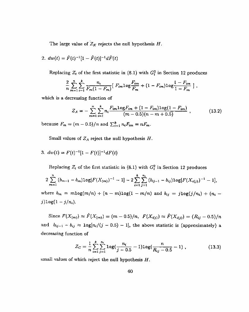
which is a decreasing function of
because Fm = (m - 0.5)/n and CL, niFi, = nFm.
Small values of ZA reject the null hypothesis H.
Replacing Zt of the first statistic in (8.1) with G: in Section 12 produces
where bm = m ï o g ( m / n ) + (n - m ) ï o g ( l - m/n) and b, = j i o g ( j / n * ) + (ni -
j ) l o g ( l - j /n i ) -
Since F(X[,)) zs F(X[,)) = (rn - 0.5)/n, F(XiD-)) ̂: F(xib1) = (R, - 0.5)/n
and bij-l - bij z l og[n i / ( j - 0.5) - 11, the above statistic is (approximately) a
decreasing function of
small values of which reject the nul1 hypothesis H .

14. Power Cornparison for k-Sample Tests
For twceample tests (k=2), our simulation show that the powers of ZK, ZA and
Zc in (9.1)-(9.3) are generally rnuch higher than those of the traditional tests, which
are location-sensitive only.
In this section we will give some examples of three-sarnple tests (k=3) , which,
together with the examples of two-sarnple tests in Section 10, are illustrations for
general k-sample tests. The powers of ZK, ZC and ZA in (13.1)-(13.3) are compared
with the conventional k-sample tests Ks, A2 and W2 in (12.1)-(12.3), as well as the
Kruskal-Wallis test KLv (Kruskal and Wallis, 1952), which is a common used non-
parametric k- sarnple test. The asymptotic relative efficiency of Krv to the one-way
F test is 3 /~=0 .955 under the condition of normality, but it is usually greater than
one in the case of non-normality, Say 1.5 for exponential distributions (see Conover,
1980; Gibbons, 1992).
For the following situations about the underlying distributions under the nul1 and
alternative hypotheses, the powers of the seven statistics are approximated by Monte
Carlo simulation, where the number of replicates is 10,000, and the significance level
for testing H is CI = 0.05.
The simulated powers are plotted against the total sarnple size n = nl + n* + n3
for selected values of (nl, 722, n3): (10, 10, IO), (10, 10, 20), (10, 20, 20), (20, 20,
ZO), (20, 20, 50), (20, 50, 50), (50, 50, 50), (50, 50, lOO), (50, 100, 100), (100, 100,
100).

Example 14.1: Fl = U(0 , 1) and Fi = Beta(pi, qi) (i=2, 3)
Without loss of generality, we assume that the underlying distribution FI of the
first sample is the standard uniform U(0 , 1). Then the natural candidates for FÎ
and f i , the underlying distributions of the second and third samples, belong to
the family of beta distribution Beta@, q), which include the uniform one because
of Beta(1, 1 ) = U(0, 1). Assuming F, = Beta(pi, pi ) (2=2, 3), we can see that
the three-sample test for H : Fl = F2 = F3 is actually a parametric test for
H : ( p i ) = 1 1) (i=2, 3).
For the following cases about the alternative hypothesis:
( 1 ) FI = U(0 , l ) , F2 = Beta(O.7, 0.7) and F3 = Beta(0.5, 0.5)
( 2 ) FI = U(0 , l ) , F2 = Beta( 1 , 0.7) and F3 = Beta(0.7, 0.5)
(3) FI = U(0, l ) , F2 = Beta( 1 , 0.7) and F3 = Beta(0.7, 1 )
(4) FI = U(0 , l ) , F2 = Beta( 1 , 1.5) and F3 = Beta(l .5, 1 )
( 5 ) FI = U(0 , l ) , F2 = Beta( 1 , 1.5) and f i = Beta(l.5, 2 )
( 6 ) Fl = U(0 , 1 ) , F2 = Beta(l.5, 1.5) and F3 = Beta( 2 , 2 )
the powers of ZA, ZC, ZK, A?, W 2 , KS and Kw are plotted in Fig. 14.1 respectively.
We can see that ZA and Zc have the highest powers and dominate the others. Al-
though not as powerful as Z A and Zc, ZK i~ overwhelming compared to its analogue
K s Besides, arnong 4 2 , W2 and Ks, A2 is the best and Ks is the worst (this is

also t m e for other examples). Finally, in cases 1 or 6 where Fi (i=l, 2, 3) have
the same location (mean) but different shapes, the new statistics are much powerful
than the old ones. In such a case, the conventional Kruskal-Wallis test Kw totally
fails because its power is almost equal to a = 0.05, the significance level of the test.
Example 14.2: FI = N(0, 1) and = N(pi, a:) (i=2, 3)
Because of the importance of normal distribution, Fi (i=l, 2, 3 ) are assumed to
be normal distributions N ( p i , 0:). We can assume that Fl = N(0, 1) without loss
of generality. Then testing H : FI = F2 = F3 is equivalent to testing H : (b, O:) =
(O, 1) (i=2, 3).
Fig. 14.2 compares the powers of the seven statistics for the following situations
about the alternative hypothesis:
(1) FI = N(0, l), F2 = N ( O , 2 ) and F3 = N ( O , 4 )
(2) FI = N(0, l ) , F2 = N ( O , 2 ) and F3 = N ( O , 0.5)
(3) FI = N(0, l ) , F2 = N(0.3, 1 ) and F3 = N(0.6, 1 )
(4) Fl = N(0, l), F2 = N(0.6, 1 ) and F3 = N ( 1 , 1 )
(5) FI = N(0, l), F2 = N(0.3, 0.5) and F3 = N(0.6, 2 )
(6) FI = N(0, l) , F2 = N(0.6, 0.5) and F3 = N(0.3, 2 ).
I t is obvious that in cases 3-4 where Fi ( i=l , 2, 3) have different locations (means)

but the same dispersion (variance), there is little difference of powers between the
new statistics and the old ones. Conversely, in cases 1-2 where Fi have the same
location but different dispersions, the power improvements of the new statistics on
the old ones are tremendous. In such cases, the Kruskal-Wallis test Kw has almost
'no power' (see also other examples). Finally, in cases 5-6 where Fi have different
locations and dispersions, the advantage of the new statistics is still significant.
We can also consider a more general case where Fl = N(0, 1) and ' ( i=2 , 3)
have symmetric distributions, such as Cauchy, logistic and t distributions, but the
results are similar according to our simulation.
Example 14.3: FI = N ( p , (r2) and Fi = Gamma(ai, bi) ( i=2 , 3)
In this example FI (x) is also assumed to be a normal distribution N ( p , a2), but
Fi(x) (i=2, 3) have non-symmetric distributions, Say Gamma(ai, bï), the gamma
distributions with shape parameter ai and scale parameter bi-
Six cases about the alternative hypothesis are considered as follows:
(1) FI = N ( 3 , l ) , F2 = Gamma(3, 1) and 27' = Gamma( 6, 2 )
(2) FI = N(5, 1), F2 = Gamna(5, 1) and F3 = Gamma(i0, 2 )
(3) 4 = N(2, 3), F 2 = Gamna(3, 1) and F3 = Gamma( 5, 1.3)
(4) Fl = N(6, 5), F2 = Gamma(5, 1) and F3 = Gamma(l0, 1.4)
(5) FI = N ( 2 , 2), F2 = Gamma(3, 1) and F3 = Gamma( 5, 2 )

( 6 ) FI = N(3, 3), F2 = Gamma(5, 1) and F3 = Gamma( 8 , 2 ).
Note that Fi (2=2, 2, 3) have the sarne mean but different variances in cases 1-2,
different means but approximately the same variance in cases 3-4, different means
and variances in cases 5-6. Power comparisons are given in Fig. 14.3, the results are
almost the same as those in Example 14.2.
Similar results can be obtained if we consider such cases where Fi = N ( 0 , 1 ) and
Fi ( i=2, 3 ) have other non-symmetrïc distributions, such as log- normal, Weibull
and F distributions.
Example 14.4: FI = N(0.5, C.?) and Fi = Beta(pi, qi) (i=2, 3)
In the last example, FI = N(0.5, 0.1) but Fi = Beta(pi, qi) (i=2, 3), where F2 is
symmetric (p2 = 92) while F3 is non-syrnmetric (p3 # q3). The following situations
are considered:
( 1 ) F1 = N(0.5, 0 - l ) , f i = Beta( 2 , 2 ) and F3 = Beta( 2 , 2.5)
(2) FI = N(0.5, 0.1), F2 = Beta( 2 , 2 ) and F3 = Beta( 2 , 1.5)
(3) Fl = N(G-5, 0. l), F2 = Beta(l.5, 1.5) and F3 = Beta(l .5, 2 )
( 4 ) FI = N(0.5, 0 . l), F2 = Beta(l.5, 1.5) and F3 = Beta(l .5, 1 )
(5) FI = N(0.5, 0 - l ) , F2 = Beta( 1 , 1 ) and F3 = Beta( 1 , 1.5)
( 6 ) f i = N(0.5, 0-l), F2 = Beta( 1 , 1 ) and F3 = Beta( 1 , 0.5).

The powers of the seven statistics are exhibited in Fig. 14.4, which shows that the
new statistics are much more powerful than the old ones.
We can see from these examples that the traditional k-sample tests are sensitive
to location differences among Fi ( i= l , 2, ..., k), but are du11 to detect the variations
of their shapes. As a result, it seems that
(a) when the differences among Fi arrive from their locations or means only, the
new statistics are as powerful as the traditional ones with ZA, ZC, A2 and Kiv
being better;
(b) when the differences among Fi come not only from their locations or means
but also from their shapes (including dispersions), the new statistics are much
more powerful than the old ones; In such a case, ZA and ZC dominate the
others, ZK or A2 is the second best, and Kiv or Ks is the worst;
(c) Zh' is ovenvhelmingIy powerful compared to its analogue Ks;
(d) Among A2, W2 and Ks, the traditional k-sample tests based on EDF (empirical
distribution function), A2 and Ks are respectively the best and worst in al1
situations;
(e) the Kruskal-Wallis test Kw fails to detect the difference in shapes among Fi.
(f) ZA and Zc are almost equivalent, but Zc is the best because of its simple
representation in (13.3).

Fig. 14.1. Power cornparison for testing FI = U(0, 1) and Fi = Beta(pi, qi) (2=2,
3) at level cr = 0.05
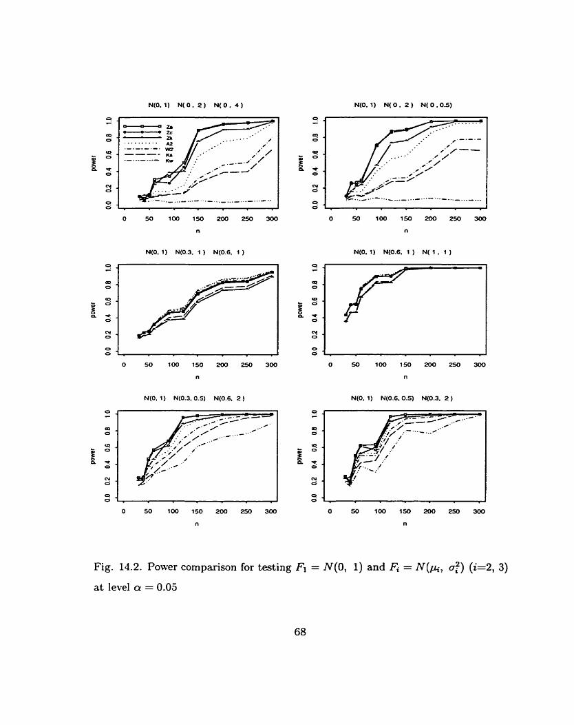
Fig. 14.2. Power cornparison for testing Fi = N(0, 1) and F, = N ( b , O:) ( i=2, 3)
at level a = 0.05

Fig. 14.3. Power cornparison for testing FI = N ( p , O*) and Fi = Garnna(ai, bi)
( i=2 , 3) at level CY = 0.05

Fig. 14.4. Power cornparison for testing FI = N(0.5, 0.1) and Fi = Beta(pi, qi)
( i=2 , 3) at level a = 0.05

15. The Distributions of k-Sarnple Za4, Zc and ZK
As the two-sample case, the k-sample statistics ZA, ZC and ZK in (13.1)-(13.3)
are distribution-free. Theîr nul1 distributions are uniformly discrete, and thus can
be obtained by enurneration of al1 possible values of the statistics by considering
n!/(nl!n2! - - nk!) combinations of the ranks R, (i = 1, 2, ..., k; j = 1, 2, ..., ni).
Note that ZA, ZC and ZK are functions of 4. Under the nul1 hypothesis H , every
combination of 1, 2, ..., n into k groups of sizes 721, na ..., nk is equally likely to be
the ranks of the k sarnples.
Since the number of values that each of the statistics can take on increases very
rapidly with ni and k, it is not feasible to give the full distribution unless and k
are small. Moreover, extensive tables have to be used for tabulating their percentage
points with different ni and k (even if they are small).
Fortunately, with today's computing facilities and software, it is easy to get
the approximate p-value of such a k-sample test by Monte Carlo simulation. The
accuracy is good enough in practice if the number of replicates (N) is sufficiently
large. In fact, the standard error of simulated pvalue is dP(l - p ) / N .
Computer programs in Splus code (Program 1-3) are given below to calculate
each new statistic and its simulated pvalue for the k-sample test. These programs
are e s y to run even on PC. For example, for a three-sample test with sizes nl=lOO
and n2=n3=ZOO: Program 1 rzquires about three minutes to run on PC (Pentium
II-MMX CPU at 300 MHz) for a 10,000-sized simulation.

In Program 1-3, M is simulation size, n = (nl, n,, ..., nk) and X is the vector
of data for the k samples, Le.,
Program 1. Cdculating Zc and its pvalue (k-sample case)
f <- function(n, X, M) {
N <- sum(n)
r <- ceiling(rank(X1)
P <- (1:N-.5)/N
W <- N* (P*log(P) + (1-P) *log(l-P))
g <- function(n,r,N,W) (
u <- O
k <- lengthh)
m <- 0:k
for (i in 1:k) (
mCi+i] <- s m ( n Ci : il )
d <- (rnci] +1) :m[i+l]
u <- u+sum(log(n[i]/(l:n[i]-.5)-l)*log(~/(sort(r[dI 1--5)-1)) 3
return(u/N) 3
Zc <- g(n,r,N,W)
z <- O
for (m in 1:M) z <- z + (g(n,rank(sample(N)),N,W) < Zc)

p.value <- z/M
returnczc , p. value) 1
f( ~ (10, 20, 201, ninif(50), 100 )
Program 2. Calculating ZA and its pvalue (k-sample case)
f <- function(n, X , M) (
N <- sum(n)
r <- ceiling(rank(X))
P <- (1:N-.5)/N
W <- N* (P*log(P) +(1-P) *log(l-P) )
g <- function(n,r,N,W) (
u <- rep(0,N)
k <- length(n)
m <- 0:k
f o r (i in 1:k) ( m[i+l] C- sum(n[l:i])
d <- (m[il+i) : m [ i + l ]
d <- sort (r [dl )
D <- ~ ( 1 , d, N+I)
p <- rep(O:n[i], DC2:(nCi]+2)]-D[i:(nCiJ+1)1)
pCdl <- pcdl--5
p <- p/nCil

u <- u-n [il * (p*log(p+. 000000001) +(1-pl *log(l-p+ . 000000001) ) 3
return( sum(u/(l:~-.s)/(N:I-.5)) ) 3
Za <- g(n,r,N,W)
z <- O
for (m in l:M) z <- z + (g(n,rank(sample(N)),N,W) < Za)
p . value <- z/M
return(Za, p. value) 1
f( c(10, 20, 201, runif(50), 100 )
Program 3. Calculating ZK and its pvalue (k-sample case)
f <-function(n, X , M) {
N <- sum(n)
r <- ceiling(rank(X))
P <- (1:N-.5)/N
W <- N* (P*log(P) +(1-P) *log(l-P) )
g <- function(n,r,N,W) C
u <- rep(0 ,NI
k <- length(n1
m <- 0:k
for (i in 1:k) ( rn[i+l] c- sum(n[l:i])
d C- ( r n [ i ] + i ) : m [ i + l ]

d <- sort (r [dl
D <- c(1, d, N+1)
p <- rep(O:nCi], D[2:(n[i1+2)1-DCl:(n~il+l)~)
pCdl <- p k W . 5
p <- phCi1
u <- u+n[i]*(p*log(p+.000000001)+(1-p)*log(l-p+.000000001)) > returd max(u-W) )
Zk <- g(n,r,N,W)
z <- O
for (m in L M ) z <- z + (g(n,rank(sample(N)),N,W) > Zk)
p .value <- z/M
return(Zk, p.value) )
f( c(10, 20, 20), ninif(50), 100 )
16. Beta Approximation to the Distribution of Ks
Although the sampling distributions of EDF tests are intractable, sometimes
they can be approximated by a simple distribution family. As a simple example, we
now consider the Kolmogorov-Smirnov statistic Ks in Section 2.
The asymptotic distribution of Ks under nu11 hypothesis was derived by Kol-
mogorov (1933), and Smirnov (1939) gave a simpler proof. However, the exact null
distribution for finite-sample case is complicated to express. Kolmogorov (1933)
and Massey (1950) established recursive formulas for calculating the null probabil-
ity P ( K s < k / n ) for integer values of k. Then Bimbaum (1952) tabulated these

values for n=l , 2, ..., 100 and k=l, 2, ..., 15.
Since the exact nul1 distribution of Ks is only available a t kln for limited integer
values of k, approximate methods have been explored. For example, some critical
values of Ks based on interpolation were given by Massey (1951) and Birnbaum
(1952), and the most common-used approxirnate critical values in statistical tables
and literature were from Miller (1956). However, the approximation is only valid
for the upper tail of the distribution, since the cnticd values (with level a) are
approxirnated by the exact ones (with level 4 2 ) for one-sided test. See Conover
(1980) and Gibbons (1992).
Research on the Kolmogorov-Smirnov statistics and their sampling distribu-
tions remains very active. See, for instance, Cabaiia (1996), Cabaiia and CabaÏia
(1994,1997), Friedrich and Schellhaas (1998), Justel, Peiïa and Zamar (1997), Kim
(1999), Kulinskaya (EM) , Paramasamy (1992) and Rama(1993) among others.
In the following we will show that the distribution of the Ks can be globally
approximated by a general beta distribution. The approximation is very simple and
reliable. Therefore, we may use a beta distribution to find the practical p-value of
the Ks test.
On the other hand, tradi tional methods of appro-ximating the p-value are more
complicated and Iess accurate. For example, the current approximation method
used in S-Plus is based on interpolation for small sample (n 550) or the limiting
distribution for n > 50, which is not be accurate enough.
Let Bp, , denote a random variable having standard beta distribution Beta@, q)

with density
and distribution function
where B@, q) is beta function with p, q > 0.
Our simulation study shows that the distribution of Kolmogrov-Smirnov statistic
Ks approximately equals that of a general beta variable aBpl , + b, where constants
a, b, p, q are chosen such that Ks and aBpl , + b have the same first four moments,
or equivalently have the same mean p, standard deviation o, skewness ri = &/a3
and kurtosis r2 = ,iiq/o4, where denotes the k-th central moment.
Let p,, a,, ml and rn:! be, respectively, the mean, standard deviation, skewness
and kurtosis of Ks. It is easy to prove that Ks and aBpl , + b ( a > O) have the same
mean, standard deviation, skewness and kurtosis (or equivalent Iy have the same first
four moments) if and only if
Note that
p + q = P(rnl, rn2) with P = P(z , y) = 6 ( ~ - xZ - 1)/(3x2 - 2~ + 6),
p q = Q(rni, rn2) with Q(z, 9) = 4P2/[16 + x Z ( p + 2)'/(P + 1)]-

Hence, a, b, p, q (a > 0) are uniquely decided by
Shen Ks and aB,, , + b have the exactly same first four moments, as well as
the approximately same moments of higher order based on our simulation (see be-
low). Therefore, they have approximately the same moment generating function or
characteristic function, and thus they have approximately the same distribution.
As a result, FKs(x) and fKs(x), the distribution and density functions of Ks,
can be simply approximated by those of a%, , + b , i.e.
where a, b, p, q are given by (16.1) and will be approximated by (16.3).
Usually, having the same first four moments is not enough to guarantee a very
good approximation, but (16.2) is a special case where the two distributions also
have sufficiently close moments of higher orders and thus have approximately the
sarne moment generating or characteristic function. For n=10, 100 and 1000, for
example, the first ten standard moments of the two variables are listed in Table
16.1, where the upper numbers in double entries are the moments of I(s based on
simulation with size of one million, and the lower nurnbers correspond to aBp, + b.
The specific values of a, I , p, q are given in Table 16.2 below.
It can be seen from Table 16.1 that they do have the same first four moments
and similar moments of higher orders. Unfortunately, the exact first four moments
of Ks are not avaiIable to detemine a, 6, p, q, so we use Monte Carlo approach.
For some selected values of n, Table 16.2 Iists the first four standard moments of f i
obtained by a one-million-size simulation together with the corresponding values of
a, 6 , p, q calculated from (16.1).

TABLE 16.1. The first ten standard moments of Ks and aBP, , + b
TABLE 16.2. The first four standard moments of Ks and corresponding a, b, p, q
Since Ks is distribution-free, its moments depend only on n, so do a, 6 , p, q
in (16.1). For simplicity, linear functions of n-' and nd (d is hed) are used to

approximate them. Of course, better approximations may be made by using more
complicated functions at the price of the simplicity.
Directly fitting the data of a, b, p, q in Table 16.2 does not work weI1 and
could destroy their structure in (16.1) which enable the approximate distribution to
have correct first moments. Instead we fit the moments first. A linear regression
model y = + ,üin-l + &nd is used to fit (by least squares approach) the data of
p,,, on, rnll in2 (against n) in Table 16.2 respectively. For different values of d , we
have different models to fit the data. We choose a d which roughly corresponds to
the best fit by the following approach. One can choose any initial value of d, and
then fit the model to the data. If the fit is satisfactory, stop. Othenvise, increase or
decrease the value of d and fit the model again. Then choose the d which corresponds
to a better fit. Repeat this pocess until a satisfactory fit is obtained. In this way,
the best d can be roughly reached within a few steps by our experience. The results
are as follows:
Then, using them u the mean, standard deviation, skewness and kurtosis of Ks,
we can get a new set of data for a, b, p, q (against n) via (16.1). The new data is
well fitted by

I â = 0.003326 - 6.012/n + 5.52/n0-53
b = -0.0004245 - 0.003397/n + 0 . 3 2 0 4 / n ~ - ~ ~
p = 3.258 - 3.727/n + 4.607/nl-~
d = 25 - 161.2/n + 162.2/n'-~,
which thus well keeps the original structure of (16.1).
With a, b, p and q approximated by (16.3) the distribution of Kolmogorov-
Smirnov statistic Ks can be simply approximated by a completely known beta
distribution in (16.2).
We now discuss the accuracy of the approximation. For n=10, 50, 100, 200 and
500, Table 16.3 lists three sets of percentage points of Ks for comparison. The first
line in multiple entries is obtained from (16.2) with a, b, p and q given in (16.3); the
second line is based on a Monte Car10 simulation of size 100,000; the third line lists
the most cornmon-used approximate values given by Miller (1956), which are only
available for upper tail (asymptotic values are used if n > 100). See also Conover
(1980) and Gibbons (1992).

TABLE 16.3. Percentage points for Ks
It can be seen from Table 16.3 that (a) compared with the simulation results, Our
approximate values are very accurate in the whole region (lower, central and upper
parts) of the distribution, and the higher the percentage level, the more accurate the
approximation; (b) at the upper tail they are consistent with Miller's approximate
results for n a100 but are better than asymptotic values, which are always a little
bit larger than real ones, especially when n 5200.
The exact sampling distribution of Ks is complicated. Kolmogorov (1933) and
Massey (1950) established recursive formulas for calculating the nul1 probability

P(Ks < k / n ) for integer values of k. Note that the recursive formulas only apply to
integer k. Birnbaum (1952) tabulated these values for n=l, 2, ..., 100 and k=l, 2,
..., 15. We can use Birnbaum's tables to check the accuracy of Our approximation.
Below are such exact values for n=40 compared with the values obtained by the
beta approximation given by (16.2):
It can be seen that the values corresponding to the same k are almost equal, espe-
cially for large k. The situation is similar for other sample sizes.
exact
appr.
We conclude from above that (16.2) gIobally gives very simple and accurate
approximations to the distribution and density functions of KSI especially a t the
upper tail (the most important part). Hence, we can easily use a beta distribution
to find the practical pvalue of the Kolmogorov-Smirnov test, which is simpler and
more accurate than existing rnethods in the literature. For example, the current
approximation method used in S-Plus is based on interpolation on limited values of
exact distribution for small sample (n 550), or the limiting distribution for n > 50,
which has been shown in Table 16.3 that it may not give a good approximation to
the true value if n < 200.
-0345 -2182 .4808 .7016 -8471 -9295 ,9708 -9891 ,9964 .9989
-0344 -2224 4 1 2 .7021 -8488 -9311 -9716 -9894 .9964 .9989
17. A Simple Distribution Family

In order to generalize the approach in the previous section, we now consider a
family of distributions V(u, b, p, q, c, d) generated by the random variable
where 1. Y - Beta(p, g ) , a beta distribution with parameters p and q and pY =
E(Y) ;
2. a > O and b are constants;
3. Z has the density defined by a simple step function
with G, d > O as constants, i = 1,2,. . . ,1, satisfying ~ f = , y = I ;
4. Y and Z are independent.
For any function h(y), denote h(b) - h(a) by [ h ( y ) ] ~ t . After some routine
calculation, we can find the distribution function of V as follows .
where t = (x - b)/a, ti = pY + tdi and B,, ,(y) is the distribution function of
B W P , d-
Suppose that a random variable X has complicated distribution but finite mo-
ments pf = E ( X k ) , k=l , 2, 3, 4. Let the skewness and kurtosis of X denoted by
= p f / ( ~ f ) ~ / ~ and r$ = pf/(&x)2 respectively, where jif is the k-th central
moment (about the mean). We wish to approximate the distribution function of X
by a member of the family L'(a, b, p, q, c, d). We do this in two steps.

We choose the constants a, b, p, and q such that X has the same first four
moments as those of V in (17.1).
First, we let them have the same skewness and kurtosis, i.e.
I/z 3/2 I / z 2 1/z r r = r l = ~ f ( ~ ) and r2 =r2 =r$(cl, ) /p4 ,
where
Since Y has beta distribution, we have the following:
Substituting r r and 7; in (17.6) with rl and r 2 in (17.4), we can solve for p and q.
Hence,
with q > p (q 5 p) if rl > O (rl 50).
Second, we let X and V have the same mean and variance, which can be easily
achieved by choosing
where ji; = pq/(p + q ) 2 / ( p + q + 1)- l

Now we have already fked a, b, pl and q so that X and V in (17.1) have the
same first four moments. We use (17.3) to approximate the distribution function of
X.
Generally speaking, having the same first four moments is still not sufficient to
guarantee a very good approximation. Therefore, we use ci, i = 1 , 2 , . . . ,1, and d of
the step function (17.2) as tuning parameters for further improvement.
The construction of (17.1) is based on the following: (1) beta distributions have
different (but not arbit.rary) kinds of shapes so that Y plays a key role in controlling
the basic shape (skewness and kurtosis) of the approximate distribution; (2) step
functions can approach any density function so that Z works weil as an adjustment;
(3) a and b are scale and lacation parameters. Besides, beta distributions have the
excellent property (1 7.6), while using step functions as densities makes (1 7.3) and
(17.5) simpIe.
It is obvious that the iarger the nurnber of steps (1) we use, the more accurate
the approximation can be made, but, on the other hand, the more difficult to tune
the parameters. Also, small I makes both (17.3) and (17.5) simple.
If higher order moments of X are known, we can choose the tuning parameters
in (17.2) to match the higher order moments of X with V ( a , 6 , p, g, cl d ) . If
higher order moments are cot known, but some quantiles of X are available through
simulation or other methods, we can determine the tuning parameters to match the
quantiles. Examples are presented in Sections 18 and 19, where we fit a member

of the family V ( a , b, p, q, c, d) to Cramér-von Mises and Waston's statistics for
goodness of fit.
18. Approximate distribution for Crarnér-von Mises Statistic
The exact nul1 distribution of the classical Cramér-von Mises statistic W 2 in
Section 2 is not known except for n = oo and n=1-7 (see, e-g., Anderson and Darling
(1952)' Marshall (1958), and Knott (1974)). So, some approximate methods have
been explored.
Using the first four moments (about the mean) of W2,
Pearson and Stephens (1962) obtained some approximate percentage points for n=5,
10 and oo by fitting Johnson's SB curve, which can only give approximately the same
first four moments but requires extensive computation.
Tiku (1965) used a+ bx; to get a simple approximation by choosing a, b, and p to
give the same first three moments as above. The method is easy to apply and gives
good results a t the upper tail of the distribution, but it fails at the lower tail. This
is not surprising because the first three (or even four) moments are not sufficient to
detennine a distribution.

Stephens (1970) gave an empirical way to approximate the upper (lower) 100a%
percentage point of W2 by Ua/(l + 1/n) + O.4/n - 0.6/n2 (L,/(l+ 0.5/n) + 0.03/n),
where LI, (L,) is the corresponding point of W . . This method works very well
a t both upper and lower tails. However, it is not suitable for the central part of
the distribution. For instance, since U0.25=0.20939, the corresponding approximate
value for W: is 0.22812, but the true value is 0.21087.
The best known approximate results are given by Csorg6 and Faraway (1996).
Using one-term linking approximation to the limiting distribution and combining
many published results from literature, t hey found a sophisticated approximation
with high accuracy for al1 (upper, lower and central) parts of the distribution. The
only concern is the cornplesity of their formula. Moreover, it includes some special
functions, such as Bessel functions. Therefore i t is difficult to find the practical
p-value of a goodness-of- fit ks t .
In contrast, the method described in Section 16 is simple and can give a very ac-
curate approximation to whichever part (upper, lower or central) of the distribution.
We now discuss i t in detail as below.
Let W 2 be the random variable X in Section 17. Using its known first four
moments in (18.1), we can easily find a, b, p, and q via (17.7) and (17.8) with
, 1 2, . 1, and d fixed. Then W2 and V in (17.1) have the same first four
moments, and thus (17.3) can be used to approximate the distribution of W2.
In order to have a better approximation, we need the second step Le. the tuning
procedure for ci, i = 1,2,. . . , I , and d. How to choose the best tuning parameters

is anther topic of undergoing research. Generally speaking, the objective of tuning
parameters is to make the V and W2 have similar moments of higher orders. Unfor-
tunately, here we do not have other moments except the first four in (18.1). Another
way of tuning parameters is to let the twa variables have approximately the same
percentage points. Of course, the theoretical percentage points of W2 are unknown,
so we use Monte Carlo approach to simulate their values which are almost the same
as the approximations given by Csorgo and Faraway(l996). With simulated per-
centage points of W2, we can perform the tuning process in the following.
Since W2 has limiting distribution, we start with large sample size, Say n=1000.
First, we use one-step function (I=1) to try. With q = 1 , i t is easy to tune a single
parameter d [just several times) so that V and W2 have close percentage points as
possible. If the accuracy is not satisfactory, then use twestep function to try, but
this time we only need to tune cl and d since c2 = 1 - cl. For this example, we
finally use a four-step function with (cl, c2, CQ, c4) oc (29, 3, 1, 6 ) and d=0.84. This
configuration of parameters also works well for n=500, 200, 100, 50 and 30. For
n=20, 10, and 5, we keep using the same ci's but choose d=0.83, 0.80, and 0.72. For
simplicity, we use the following parameters for general n.
U'e spent about two hours to get this result which can be used forever. The turning
process is just like tuning a machine or equipment to fit different conditions. For
different statistics we need different parameters. In fact, it is because of the turning
parameters that make (17.1) suitable for general case.
Since a, b, p, and q have been decided by (17.7) and (17.8), by (18.2), we obtain

a complete known formula (17.3) t o approximate the distribution function of W2.
Table 18.1 lists some of these values for n=10, 50, 200, 2000, and Table 18.2 gives
the corresponding approximate percentage points (the upper numbers in double
entries) obtained from (17.3) together with those (the lower numbers) obtained by
Csorgo and Faraway (1996) for cornparison.
We can see from Table 18.2 that the two sets of numerical results are very close.
Therefore, the two approximate distributions are almost the same although they are
obtained by using different methods, and thus have totally different mathematical
expressions.
Compared with Csorg6 and Faraway's approach, our method is much simpler
without using any special function. Therefore it can be easily used to obtain practical
pvalues of goodness-of-fit tests, instead of tabulating limited percentage points.
Moreover, the approximate function in (17.3) is a real distribution function. Finally,
our method is of generality and can be applied to approximate the distribution for
a general continuous random variable with known finite first four moments.
Remark: (18.2) is just a simple solution. It is not difficult to find a better config-
uration of q and d if we let y Vary with n (like d ) . Besides, increasing 1, the number
of steps in (17.2), can absolutely raise the degree of accuracy of approximations, but
our formulas will be more complicated.

TABLE 18.1. Some values of a, 6, p, q
TABLE 18.2. Some percentage points for W 2
19. Approximate Results for Waston's Statistic

The Waston's statistic
is a modification to the Cramér-von Mises statistic IV2 so that it can test the good-
ness of fit on a circle.
Like Cramér-von Mises statistic, LJ2 is distribution-free. The exact distribution of
U2 was given by Watson (1961) for n = m and by Stephens (1963, 1964) for n=l, 2,
3, and 4. Approximate approaches based on moments or empirical estimation have
been studied by Pearson and Stephens (1962), Tiku (1965) and Stephens (1970).
The results are similar to those for W2 (see Section 17). Again, the best known
approximate results were given by Csorgo and Faraway (1996).
Nom, using the first four moments (about the mean) given by Stephens (1963):
pi = 1/12
P2 = (1 - l/n)/360 (19.1)
p. = (2 - 5/n + 3/n2)/7560
jï4 = (19 - 70/n + 8ï/n2 - 36/n3)/302400 , we apply the method in Section 16 to u*, which has lower skewness and kurtosis
than those of W 2 : but this time ive just need a three-step function (17.2) (1=3).
Results parallel to those of W2 in Section 18 are given below. We can see again
from Table 19.2 that Our numerical results are very close to those given by Csorgo
and Faraway (1996).

TABLE 19.1. Some values of a, 6 , p, q
TABLE 19.2. Some percentage points for U2
20. Concluding Rernarks
Through the parameterization introduced in Section 1, a nonparametric goodness-
94

of-fit test is simplified to a family of parametric tests. As a result, more general
types of EDF tests for goodness of fit can be defined, which include traditional EDF
tests, as well as new EDF tests Sased on the likelihood ratio. This rnethodology for
goodness-of-fit tests in Sections 1-5 is sumrnarized in Zhang (2001a).
Besides, instead of testing for a specific distribution, the new statistics can be
applied t o test the goodness of fit for a family of distributions, such as the families
of normal, exponential, gamma, and Weibull distributions. For instance, the new
tests outperform the best tests of normality in literature by simulation (see Sections
5-6). Another interesting topic is to test multivariate normality.
The methodology of goodness-of-fit tests has been developed and applied to gen-
eral two-sample and rnulti-sample problems, and parallel results have been obtained.
The simulations in Sections 8-15 show that the new tests are sensitive to the dif-
ference in location, scale and shape among distributions, while traditional tests are
du11 to detect the variation in shape or scale. The major results of the two-sample
tests in Sections 8-10 are given in Zhang (2001b).
Since the exact sarnpling distributions of the EDF test statistics are intractable,
we have to investigate some approximate approaches. In Sections 16-19, a sim-
ple distri but ion family is introduced to approximate the distribution function for a
general continuous randorn variable. When applied to some EDF test statistics, it
gives similar numerical results as the best known, but it is much sirnpler and can
be directly used to o5tain prxtical p-values of goodness-of-fit tests (Zhang and Wu,
2001a, 2001b). The key issue in using simple distribution family is choosing the
tuning parameters involved. This is still an area of on-going research.

References .
Anderson, T. W. and Darling, D. -4. (1952) Asymptotic theory of certain "goodness
of fit" criteria based on stochastic processes. Ann. Math. Statist., 23, 193-212.
Anderson, T. W. and Darling, D. A. (1954) A test of goodness of fit. J. Amer.
Statist. Assoc. 49, 765-769.
Anderson, T. W. (1962) On the distribution of the two-sample Cramér- von Mises
criterion. Ann. Math. Statist., 33, 1148-1 159.
Baumgartner, W., Weip, P. and Schindler, H. (1998) A nonparametric test for the
general two-sample problem. BiometBcs, 54, 1129- 1 135.
Birnbaum, Z. W. (1952) Numerical tabulation of the distribution of Kolmogorov's
statistic for finite sample size. J. Amer. Statist. Assoc. 47, 425-441.
Birnbaum, Z. \IV. and Tingey, F. H. (1951) One-sided confidence contours for prob-
ability distribution functions. Ann. Math. Statist., 22, 595-596.
Burr, E. J. (2963) Distribution of the two-sample Crarnér-von Mises criterion for
small equal samples. Ann. Math. Statist., 34, 95- 101.
Burr, E. J. (1964) Small-sample distributions of the two-sample Cramér-von Mises
W 2 and Watson's U2. Ann. Math. Statist., 35, 1092-1098.
Cabana, A. (1996) Transformations of the empirical rneasure and Kolmogorov-
Smirnov tests. Ann. Statist., 24, 2020-2035.

Cabana, A. and Cabana, E. M. (1994) Goodness-of-fit and cornparison tests of
the Kolmogorov-Smirnov type for bivariate populations. Ann. Statist., 22,
1447-1459.
Cabafia, A. and Cabafia, E. M. (1997) Ransformed empirical processes and mod-
ified Kolmogorov-Smirnov tests for multivariate distributions. Ann. Statist.,
25, 2388-2409.
Conover, W. J. (1965) Several k-sample Kolmogorov-Smirnov tests. Ann. Math.
Statist., 36, 1019-1026.
Conover, W. J. (1980) Pructical Nonparamethc Statistics, 2nd ed. New York: John
Wiley.
Cramér, H. (1928) On the composition of elementary errors: II, Statistical appli-
cations. Skand. Alct. 11, 14:-180.
Cressie, N. and Reed, T. R. C. (1984) Multinomial goodness-of-fit tests. J. R.
Statist. Soc. B, 46, 440-464.
Csorgo, S. and Faraway, J. J. (1996) The exact and asymptotic distributions of
Cramér-von Mises statistics. J- R. Statist. Soc. B , 58, 221-234.
D'Agostino, R. B. (1971) An omnibus test of normality for moderate and large
sample size. Biometrika 58, 341-348.
D7Agostino, R. B. (1973) Monte Car10 power cornpanson of the W' and D tests of
normality. Comm. Statist. 1, 545-551.
D7Agostino, R. B. and Stephens, M. A. (1986) Goodness-of-Fit Techniques. New
York: Marcel Dekker.

Darling, D. A. (1957) The Kolmogorov-Smirnov, Cramér-von Mises tests. Ann.
Math. Statist., 28, 823-838.
Dudewicz, E. J. and van der Meulen, E. C. (1981) Entropy-based tests of unifor-
mity. J. Amer- Statist. Assoc- 76, 967-974.
Dyer, A. R. (1974) Cornparisons of tests for norrnality with a cautionary note.
Biometrika 61, 185-189.
Epps, T. W. and Singleton, K. J. (1986) An omnibus test for the two- sample
problem using empirical characteristic function. J. Statist. Comput. SimuL,
26 177-203.
Ferger, D. (2000) Optimal tests for the general two-sample problem. J. Multivariate
Anal., 74, 1-35.
Friedrich, T. and Schellhaas, H. (1998) Computation of the percentage points and
the power for the twssided Kolmogorov-Smirnov one sample test. Statist.
Papers, 39, 361-375.
Gibbons, J. D. (1992) Nonpararnetric Statistical Inference, 3nd ed. New York:
Dekker.
Gnedenko, B. V. (1954) Tests of homogeneity of probability distribution in two
independent samples (in Eussian). Doklody Akademii Nuuk SSSR, 80, 525-
528.
Hcijek, J. and Sidak, Z. (1967) Theory of Rank Tests, Academic Press, New York.
Hall, P. and Padmanabhan, A. R. (1997) Adaptive inference for the two- sample
scale problem. Technometrics, 39, 412-422.

Hodges, J. L. Jr. (1958) The significance probability of Smirnov two- sarnple test.
Arkivfoer Matematik, Astronomi och Fysik, 3, 469- 486.
Justel, A., Peiia, D. and Zamar, R. (1997) A multivariate Kolmogorov- Smirnov
test of goodness of fit. Statist, Probab. Lett., 35, 251- 259.
Kiefer, J. (1959) K-sample Analogues of the Kolmogorov-Smirnov, Cramér-von
Mises tests. Ann. Math. Statist., 30, 420-447.
Kim, T. Y. (1999) On tail probabilities of Kolmogorov-Smirnov statistics based on
uniform mixng processes. Statist. Probab. Lett., 43, 217-223.
Knott, M. (1974) The distribution of the Cramér-von Mises statistic for small
sample sizes. J. R. Statist. Soc. B, 36, 430-438.
Kolmogorov, A. (1933) Sulla determinazione empirica di una legge di distribuzione.
Giom. Inst. Ital. Attuari. 4, 83-91.
Kruskal, W . H. and Wallis, W. A. (1952) Use of ranks in one-criterion analysis of
variance. J. Amer. Statist. Assoc., 47, 583-62 1; errata, ibid., 48, 907-91 1.
Kulinskaya, E. (1995) Coefficients of the asymptotic distribution of the Kolmogorov-
Smirnov statistic when parameters are estimated. J. Nonpararnetr. Statist.,
5 , 43-60.
Marshall, A. W. (1958) The small sample distribution of nw$ Ann. Math. Statist.,
29, 307-309.
Massey, F. J. (1951) The Kolmogorov-Smirnov test for goodness of fit. J. Amer-
Statist. Assoc., 46, 68-77.

Massey, F. J. (1952) Distribution table for the deviation between two sarnple cu-
mulatives. Ann. Math. Statist., 23, 435-441.
Miller, L. H. (1956) Table of percentage points of Kolmogorov statistics. J. Amer.
Statist. Assoc. 51, 111-121.
von Mises, R. (1931) Wahrscheinlichkeitsrechnung und Ihre Anwendung in de
Statistik und Theoretischen Physik. Leipzig: Deuticke.
Nair, V. N. (1984) On the behavior of some estimators frorn probability plots. J.
Amer. Statist. Assoc., 79 , 823-830.
Pearson, E. S. and Stephens, M. A. (1962) The goodnessof-fit tests based on W$
and U;. Biometrika, 49, 397-402.
Pettitt, A. N. (1976) A two-sample Anderson-Darling rank statistic. Biometrika,
63, 161-168.
Paramasamy, S. (1992) On the rnultivariate Kolmogorov-Smirnov distribution.
Statist. Probab. Lett., 15, 149-155.
Pratt, J. W. and Gibbons, 3. D. (1981) Concepts of Nonparametric Theory, Springer-
Verlag, New York.
Rama K. Y. S. (1993) On tail probabilities of Kolmogorov-Smimov statistic based
on strong mking processes. Statist. Probab. Lett., 16, 369-377.
Reed, T. R. C. and Cressie, N. (1988) Goodness-of-Fit Statistics for Discrete Mul-
tivariate Data. Nork York: Springer-Verlad.

Scholz, F. W. and Stephens, M. A. (1987) K-sample Anderson-Darling tests. J.
Amer. Statist. Assoc., 82, 91û-924.
Shapiro, S. S. and Francia, R. S. (1972) Approxïmate analysis of variance test for
normality. J. Amer. Statist. Assoc. 67, 215- 216.
Shapiro, S. S. and Wilk, M. B. (1965) Analysis of variance test for normality
(complete samples). Biometrika 52, 591-61 1.
Shapiro, S. S. and Wilk, M. B. (1968) Approximation for the nul1 distribution of
the t V statistic. Technometrics IO? 861-866.
Shapiro, S. S., Wilk, M. B. and Chen H. J. (1968) -4 comparative study of vanous
tests for normality. J. Amer. Statist. Assoc. 63, 1343-1372.
Sinclair, C. D. and Spurr, B. D. (1988) Approximations to the distribution function
of Anderson-Darling test statistic. J. Amer. Statist. Assoc. 83, 1190-1 191.
Smirnor, N. V. (1936) Sur la distribution de w2 (critérium de M. R. v. Mises). C.
R. Acad. Sci. Paris, 202, 449-453.
Smirnov, N. V. (19371 On the distribution of Mises' u2- criterion (in Russian).
Mat. Sb. (Nov. Ser.), 2, 973-993.
Srnirnov, N. V. (1939) Estimate of derivation between empirical distribution func-
tions in turo independent samples (in Russian). Bulletin of Moskow University,
2, 3-16.
Spinelli, J. J . and Stephens, M. A. (1997) Cramér-von Mises tests of fit for the
Poisson distribution. Canad. J. Statist. 25, 257-268.

Stephens, M. -4. (1963) The distribution of the goodness-of-fit statistic U;. 1.
Biometrika, 50, 303-313.
Stephens, M. A. (1964) The distribution of the goodness-of-fit statistic, G. II. Biometrika: 51, 393-397.
Stephens, M. A. (1970) Use of the Kolmogorov-Smirnov, Cramér-von Mises and
related statistics without extensive tables. J. R. Statist. Soc. B, 32, 115-122.
Stephens, M. A. (1974) EDF statistics for goodnessof-fit and some comparisons.
J . Amer. Statist. Assoc. 69, 730-737.
Stephens, hl. A. and Maag, U. R. (1968) Further percentage points for IV$.
Biometrika, 55, 428-430.
Tiku. M. L. (1965) Chi-square approximations for the distributions of goodness-of-
fit statistics U s and L V ~ . Biometrika, 52, 630-633.
Watson G. S. (1961) Gocdness-of-fit tests on a circle. Biometrika, 48: 109-1 14.
Wolf, E. H. and Naus, J. 1. (1973) Tables of critical values for a Ir- sample KoIrnogorov-
Smirnov test statistic. J. Amer. StatZst. Assoc., 68, 994997.
Zhang, J. (2001a) Powerful goodness-of-fit tests Sased on likelihood ratio. J. R.
Statist. Soc. B, in revision.
Zhang, J . (200 1 b) Powerful general two-sample tests. Technornetrics, in revision.
Zhang, J . and Wu, Y. (2001a) Beta approximation to the distribution of Kolmogorov-
Smirnov statistic. Ann. Inst. Stattis Math., in revision.

Zhang, J. and Wu, Y. (2001b) A family of simple distribution functions to approx-
imate complicated distributions. J. Statist. Corn. S h . , to appear.