6goodness of fit tests

CHAPTER 5

GOODNESS OF FIT TESTS

"...it is important that the particular goodness of fit test used be se-lected without consideration of the sample at hand, at least if the calculatedsignificance level is to be meaningful. This is because a measure of dis-crepancy chosen in the light of an observed sample anomaly will tend to beinordinately large."

H.T. David, 1978

Prior to the interest in tests specific to identifying non-normality, initiatedat least in part by the test of Shapiro and Wilk (1965), distributionalassumptions were verified most often by more general goodness of fit testswhich could be used for any simple null hypothesis FQ(X). These tests areunique from the tests for normality described in the preceding chaptersin that, under a simple hypothesis, their distribution is independent ofthe null distribution and therefore tables of critical values are identicalregardless of the hypothesized null distribution. However, prior knowledgeof distributional parameters is relatively rare in actual practice.

In general, the goodness of fit tests described here rely on the relationof the empirical distribution function of the observations to the hypothe-sized distribution function in some manner: e.g., by direct comparison, asin the Kolmogorov-Smirnov test; by comparing the number of actual withthe expected number of observations occurring within bins defined by the

Copyright © 2002 by Marcel Dekker, Inc. All Rights Reserved.

null distribution, as in the x2 test; or by comparing spacings within thenull distribution function.

It was not until relatively recently that null distributions or criticalvalues of many of these tests were obtained for use with a composite nullhypothesis. If FQ(X) is completely specified, then pi = -Fo(zj) are uniformrandom variables; however, if one or more parameters are unknown, thenthe pi obtained using estimated parameters are no longer uniform. If FQ(X)depends only on a location and scale parameter, then the distribution ofFo(x\0) under the null hypothesis depends on the functional form of FQ(X),but not the parameters (David and Johnson, 1948; Stephens, 1986a).

In this chapter we will focus on general goodness of fit tests and theirapplication to testing for normality when parameters are unknown. Whilewe attempt to mention as broad a range of tests as possible, we will beconcerned mainly with those tests that have been shown to have decentpower at detecting normality; less powerful tests will be described in lessdetail, except for those with historical interest.

5.1 Tests Based on the Empirical Distribution Function

Empirical distribution function (EDF) tests are those goodness of fit testsbased on a comparison of the empirical and hypothetical distribution func-tions. There are two general types of EDF test: those based on themaximum distance of empirical to null distribution function (Kolmogorov-Smirnov test and Kuiper's V), and quadratic tests (Anderson-Darling andCramer-von Mises tests). As originally derived, these tests require a sim-ple rather than compound hypothesis. More recently (Lilliefors, 1967;Stephens, 1974) they were expanded to include those circumstances wherethe mean and variance were not specified, and these have been shown tohave power which was comparable to the Wilk-Shapiro test for some alter-natives to normality.

The EDF of a sample, designated Fn(x], is a step function defined as

{ 0 x < x(l)

i/n x(i} <x < x(i+l} i = 1, . . . , n - 1I x(n} < x.

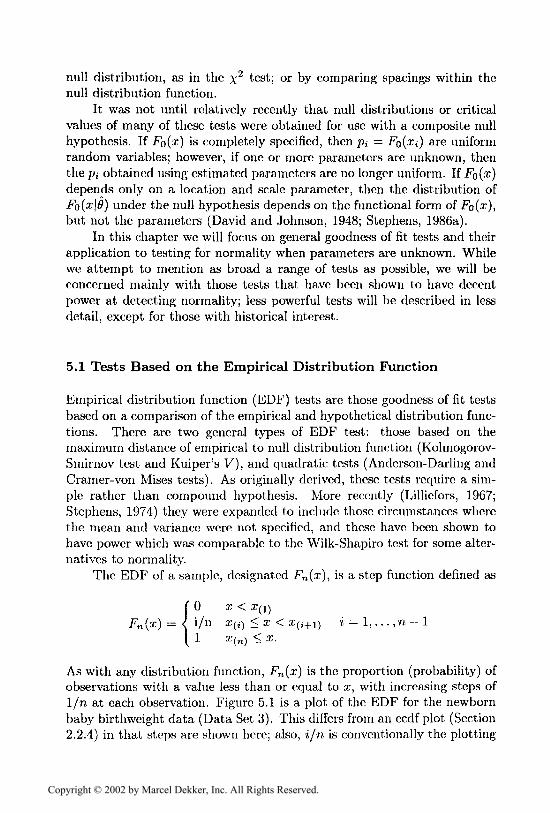
As with any distribution function, Fn(x) is the proportion (probability) ofobservations with a value less than or equal to x, with increasing steps of1/n at each observation. Figure 5.1 is a plot of the EDF for the newbornbaby birthweight data (Data Set 3). This differs from an ecdf plot (Section2.2.4) in that steps are shown here; also, i/n is conventionally the plotting


70 80 90 100 110 120 130 140 150

Birthweights

Figure 5.1 EDF plot of newborn birthweights (n = 82).

position used in EDF plots. EDF tests are based on the differences betweenthe EDF and the distribution function based on the null hypothesis, in thenormal case p^ = ^([x^) — fi\/ff}. EDF tests reject the null hypothesis(normality) when the discrepancies between the EDF and the hypothesizedcumulative distribution function are too large; hence, these tests are allupper-tailed tests. There has been some concern that test values that aretoo small might indicate a lack of randomness in the data, and thereforelower-tailed or two-tailed tests should be used (Stephens, 1986a); however,this problem of superuniformity will not be considered here.

Although these tests can be used for p^ — FQ(X^} for any distributionFO, critical values for these tests are dependent upon the null distribution.Modifications to the EDF tests in this section have been derived (Stephens,1974) so that the critical values for each test are independent of the samplesize.

5.1.1 The Kolmogorov-Smirnov Test

The Kolmogorov-Smirnov statistics are based on the maximum differencesbetween the EDF and the p^. These are given by

D+ = max [i/n — p^)}

D~ = max [p(j) — (i — l)/n]i=l,...,n

D = max[D+, D~\.


Lilliefors (1967) was the first to address the issue of using EDF tests forcomposite hypotheses, when he investigated the null distribution of D un-der a normal composite null hypothesis and compared it to the %2 test interms of power. Lilliefors gave a table of critical values for D based onsimulation. However, for simplification, the modification

- 0.01 +

(Stephens, 1974) can be compared to the critical value of 0.895 for an 0.05level test for all sample sizes; critical values of the null distribution of D*for other levels of significance are given in Table B15.

Example 5.1. For the birthweight data (Data Set 3), the valueof D+ is found at the sixth observation and D~ is found at thefourteenth observation. These values are 0.1006 and 0.1431, re-spectively. Therefore, D = 0.1431 and

£>* = (5.66 - 0.01 -f 0.15),D = 0.830.

This value does not exceed the 0.05 level critical value of 0.895.

5.1.2 Kuiper's V

The V test (Kuiper, 1960) is also based on a combination of D+ and Z)but is obtained using the sum rather than the maximum,

V = D+ +D~

withV* = ,n + 0.05 +

having fixed distribution under the null hypothesis for all sample sizes(Stephens, 1974). V can also be used for testing goodness of fit for distri-butions on a circle. Critical values for selected levels of significance for V*are given in Table B15.

Example 5.2. From the values of D and D+ in Example 5.1, forthe birthweight data we calculate

V = 0.1431 + 0.1006 = 0.2437


0 20 40 60 80 100 120 140 160 180 200Latency Period (Days)

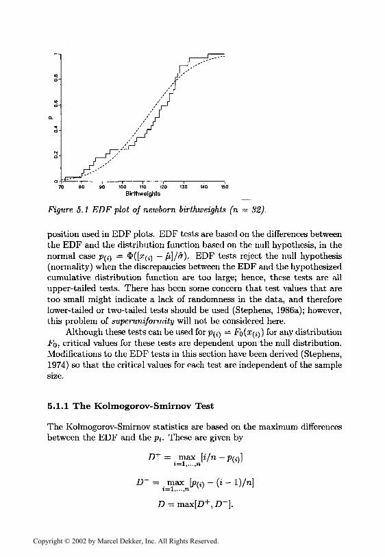
Figure 5.2 EDF plot of leukemia latency period (n = 20).

andV* = (5.66 4- 0.05 + 0.14)V = 1.426

which does not attain significance.

5.1.3 Cramer-von Mises Test

A class of EDF goodness of fit tests was proposed by Anderson and Darling(1952), defined by

n l°° [Fn(x] -J — 00

(5.1)

where i]j(F(x)) is a weighting function. In particular, the weighting func-tion i/)(F(x)) = 1 gives the Cramer-von Mises test statistic

li-l

with the modification

W2* = (1.0 + Q.5/n)W2

accounting for differences in sample size when using critical values.

Example 5.3. Figure 5.2 shows the EDF plot for the leukemia la-tency data (Data Set 9). For these data, the value ofW2 is 0.179,


resulting in the value of 0.184 for W2*. From, Table B15 we seethat this value is between the 0.01 and 0.005 level critical values,0.179 and 0.201, respectively, indicating a significant deviationfrom the normal distribution.

Critical values for W2* are given in Table B15. For distributions on acircle, Watson (1961, 1962) proposed

- ' 12n

The relationship between U2 and W2 is given by

U2 = W2 -n(p-0.5)2.

U2* = (1.0 + 0.5/n)f/2

with critical values given in Table B15.

5.1.4 Anderson-Darling Test

Anderson and Darling (1954) used tj)(p) = [p(l — p)}"1 as the weightingfunction in (5.1), resulting in the test statistic

n

l][log(p(i)) + log(l - p(n_ i+1))]

This weighting scheme gives more weight to the tails of the distributionthan does W2. Stephens (1986a) proposed the modification

A2* = (1.0 + 0.75/n + 2.25/n2)A2

to obtain a set of critical values for all sample sizes; these are provided inTable B15.

Example 5.4- The observed daily July wind speed data (Data Set8) indicate a slightly heavy-tailed distribution (b^ =4.1, see Ap-pendix 1), so the Anderson-Darling test might be more appropriatefor testing these data than other EDF tests. For these data,

A2 = 0.301


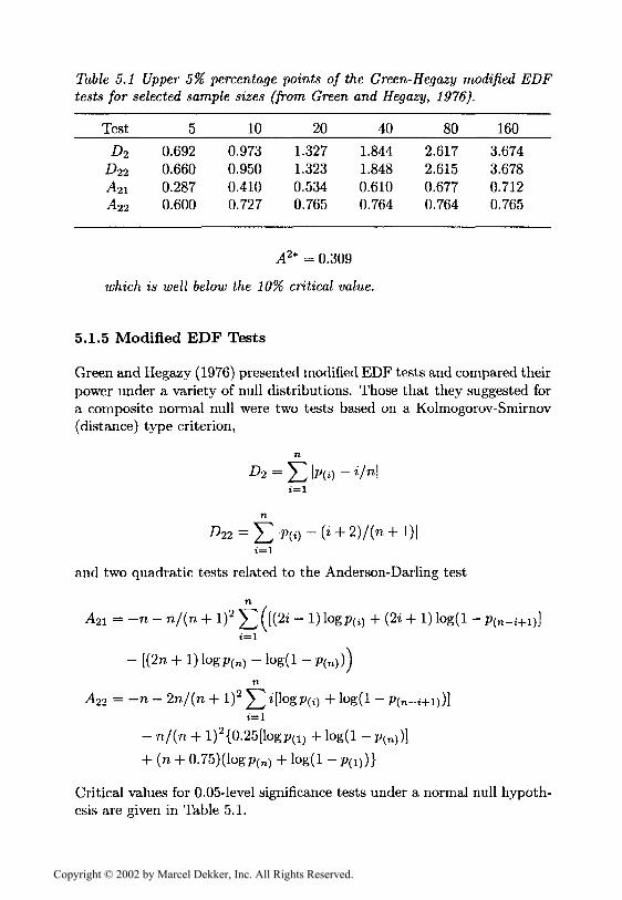
Table 5.1 Upper 5% percentage points of the Green-Hegazy modified EDFtests for selected sample sizes (from Green and Hegazy, 1976).

Test

£>2

A>2

A2\AM

50.6920.6600.2870.600

100.9730.9500.4100.727

201.3271.3230.5340.765

401.8441.8480.6100.764

802.6172.6150.6770.764

1603.6743.6780.7120.765

A2* = 0.309

which is well below the 10% critical value.

5.1.5 Modified EDF Tests

Green and Hegazy (1976) presented modified EDF tests and compared theirpower under a variety of null distributions. Those that they suggested fora composite normal null were two tests based on a Kolmogorov-Smirnov(distance) type criterion,

and two quadratic tests related to the Anderson-Darling test

n

A2l = -n - nf(n + I)2 ]£ ([(2» - 1) logpw + (2* + 1) log(l - P(n-i+i)}i=l

- [(2n + 1) logp(n) - log(l - p(n)

n

A22 = -n - 2n/(n + I)2 z[logp(j) + log(l - p(n_i

- n/(n + l)2{0.25[logm + log(l - p(n)

+ (n + 0.75)(logp(n) + log(l -

Critical values for 0.05-level significance tests under a normal null hypoth-esis are given in Table 5.1.


5.2 The x2 Test

In 1900, Karl Pearson presented his x2 goodness of fit test. Until relativelyrecently, this test was among the most useful of all tests for testing goodnessof fit, irrespective of the null hypothesis. However, with the proliferation oftests of normality that has occurred since Shapiro and Wilk (1965) providedtheir test specifically for the composite normal null, the x2 test has falleninto disfavor as a test for normality, mostly because of its lack of powerrelative to other tests for normality; Moore (1986) recommended that theX2 test not be considered "... for testing fit to standard distributions forwhich special-purpose tests are available...". Here we present a review ofthe x2 test for the purpose of historical interest and completeness.

5.2.1 Development of the x2 Test

The well known x2 goodness of fit test is given by

X = (t" " npi)' (5.2)h "•'"-and the null hypothesis is rejected for values of X2 that are too large. Toapply this test, the range of the n observations is divided into A: mutuallyexclusive classes; n,; is the number of observations that fall into class i\and pi is the probability that an observation will fall into class i under thenull hypothesis. Then npi is the number of observations which would beexpected to occur in class i. The resulting test is the familiar calculation"sum of the observed minus expected squared over the expected".

Pearson (1900) derived the test using the following reasoning: if x =(xi, ... , :Efc_i) has a nonsingular (k — l)-variate normal distribution withmean // and covariance matrix S, then the quadratic form (x—//)'S~1(x—/i)has a Xk-i distribution. For large samples (n,; — npi) is approximatelymultivariate normal, and is nonsingular if only k — 1 of the k classes areconsidered. Therefore, if X{ = n; — npi, then the quadratic form reduces to(5.2). This result holds under any null distribution.

For a simple hypothesis, this result is very straightforward, althoughthe number k and size pi of classes to use need to be considered. In addition,another important issue arises in the use of this test as a test for compositenormality: whether the distribution of the test statistic is still x2- Whenparameters are estimated, (5.2) becomes

x2 = y (n< ~ "f!0)2 (5.3)


where t is the m- vector of parameter estimates. Since the pi(t) are esti-mates of the pi, and are themselves random variables, the asymptotic Xk—idistribution no longer applies. Common practice is to use the estimates ofthe parameters to obtain the pi, calculate the test statistic and compareit to a Xfc-m-u adjusting the degrees of freedom by m. If the multino-mial maximum likelihood estimators are used to obtain the pi(t], then theasymptotic distribution is Xk-m-i (Fisher, 1924). These estimates are thesolutions to the m equations

,.i=lPi(t) 6tj

Estimators that are asymptotically equivalent to the multinomial maximumlikelihood estimators are the minimum x* estimators (Fisher, 1924), whichare the solution to the equations

and the minimum modified x2 estimators (Neyman, 1949), based on thesolution to

k^—v Pi(t) 6pi(t}2_. ~ c — 0 .7 = 1, . . . , m.z=l * ^

Since these estimators are asymptotically equivalent to the multinomialmaximum likelihood estimates, the asymptotic distribution of X2 underthese estimators is still Xk-m-i- Unfortunately, under the normal null dis-tribution none of the above estimators are able to be obtained in closedform, requiring the use of numerical optimization methods to obtain solu-tions.

When more efficient estimates are used (e.g., maximum likelihood es-timates based on the n observations rather than the multinomial estimatesbased on the k classes), the asymptotic distribution of (5.2) is no longerXfc-rn-i (Fisher, 1928; Chernoff and Lehmann, 1954). In this instancethere is a partial recovery of the m degrees of freedom lost by multino-mial estimation and so the distribution is bounded between a Xk-i anQl a

Xk-m-i distribution. For large k the difference may be ignored; however,for small k the use of a Xk-m-i may ^ea<^ *° significant error in the results.Even for k as high as twenty, which is rare in usual practice, the true sig-nificance level could be as high as 0.09 for a 5% test when estimating thetwo parameters of the normal distribution (Table 5.2).


Table 5.2 Probability levels of the xl-i distribution for the 5th percentileof the Xk.-3 distribution.

k [*\P(xl-3 > *) = 0.05} P(xl_1 > x)

56789

1520

5.997.819.49

11.0712.5921.0227.59

0.200.170.150.140.130.100.09

5.2.2 Number of Cells

One disadvantage of the %2 test is that, for a given sample, the resultsobtained from the test are affected (substantially, in some cases) by thenumber and size of the k classes chosen.

For the simple hypothesis, Mann and Wald (1942) recommended thatthe A: cells have equal probability under the null distribution, i.e., pi = l/k.This results in a more accurate approximation to the x2 distribution. Whilethe general x2 test is consistent, it is unbiased only for the equiprobable cellcase. The calculation (5.2) in the equiprobable cell case becomes simply

Kendall and Stuart (1973) showed that the best k to choose based onmaximizing the power when the power is j3 is

where za is the upper a percentage point of the standard normal dis-tribution. Mann and Wald (1942) considered the case when /3 = 0.5($~l(ft) = 0), and suggested using b — 4. Note that (5.4) suggests thatthe "best" k decreases in a region with higher power for fixed sample size,i.e., as the discrepancies (n,; — npi) get larger. However, Kendall and Stuart(1973) recommended that, for n > 200, k can be reduced by as much asone half without serious loss of power. Also, k cannot be too large sincethe normal approximation will not be adequate if the expected frequencies


are too small. They did not recommend the use of (5.4) when n < 200, inwhich case a smaller number of classes should be used. In contrast, Koehlerand Larntz (1980) claimed that the Pearson x2 test is adequate at boththe 0.05 and 0.01 levels for expected frequencies as low as 0.25 when k > 3,n > 10 and n2/k > 10.

Example 5.5. Fifty-eight wells were tested for a variety of waterquality parameters in Suffolk County, N. Y., in 1990; Data Set 10contains the observed average alkalinity of these wells. Using theKoehler-Larntz criteria, the number of cells that can be used forthese data is 232 (expected value = 0.25, n2/k = 14.5). Althoughnot recommended for n < 200, when using (5-4) to obtain k wefind that k = 79 when b = 4, and k = 40 when using 6 = 2.Based on the recommendation of equiprobable cells and that npibe greater than or equal to 5 yields k = 11, and using npi > 10(as an arbitrary alternative) yields k — 5.

Significance testing results vary widely when k = 5 and k =11. When k = 5, the value of Pearson's test is X2 = 10.5, whichexceeds both the x2 and the x2 critical values at the 0.05 levels(5.99 and 9.49, respectively). However, when 11 equiprobable cellsare used, Pearson's test is only X2 = 7.2, which is not nearlysignificant (for either 8 or 10 degrees of freedom) at even the 0.10level.

5.2.3 Other x2 Tests

Under a simple hypothesis, the likelihood ratio test statistic is

ki2G2 = 2L = 2 n{ \og(ni/nPi).

It has been shown that

, i ~ i , , / - 2 , .)-! i - i |

'" ' ' '2 npi 6

(Fisher, 1924). Ignoring all but the first term in the summation, we seethat 2L = X2 and so the likelihood ratio test statistic is asymptoticallyequivalent to (5.2) and has an asymptotic xl-i distribution. This test issubject to the same criticisms as Pearson's x2 test when parameters are


estimated. Moore (1986) recommended the use of x2 over G2 in situationswhere the hypothesis is simple or minimum x2 estimators are used.

A third type of x2 test is based on the Freeman-Tukey (1950) deviates,

which, if terms of order 1/n are omitted, reduces to

fc

(Bishop, Fienberg and Holland, 1975). FT2 is also asymptotically x2 dis-tributed. Larntz (1978) indicated that X2 more accurately approximatesthe distribution of x2 under the null hypothesis than either G2 or FT2.

5.2.4 Recommendations on the Use of the x2 Test

The use of the x2 test is not recommended as a test for univariate normality,mostly because of its lack of power. However, the flexibility of the test issuch that it is useful for testing rnultivariate normality (Chapter 9) ratherthan using other tests which are much more difficult to implement, and forcensored data (Chapter 8). A further advantage, at least over EDF tests,is the need for only one set of tables for determining significance regardlessof the form of the null distribution ^ o ^ -

5.3 Other Methods of Testing for Composite Goodness of Fit

Here we present other methods of testing goodness of fit which have beenderived specifically for composite null hypotheses. These include Neyman'ssmooth goodness of fit test modified for the composite case; using nor-malized spacings to reduce the data to (nori-uniform) ordered values onthe interval (0,1); and half- and multi-sample methods wherein psuedo-independent estimates of the parameters are used as the true values.

5.3.1 Neyman's Smooth Goodness of Fit Tests

Thomas and Pierce (1979) presented modified smooth goodness of fit tests(Neyman, 1937) which are applicable when the distribution parameters are


Table 5.3 Coefficients ams for calculating modified Neyman smooth good-ness of fit test statistics.

m/s 1 2 3 4

1234

16.3172-27.380989.7593

-118.2638

_27.3809

-156.6001436.8700

_-

104.4001-637.2124

_

--

318.6062

unknown. The smooth tests are based on a sequence of sums of individualsingle degree of freedom x2 tests, so that the jth test statistic is (at leastasymptotically) x]- Letting ?/,; = $[(£; — A)/<5"], define

s=l

Then the kth modified smooth test statistic, Wk, is

H4=£^m=l

so that Wk = Wk-i + t%- Wk can be compared to a %2 distribution withk degrees of freedom to determine significance, achieving good agreementwith the asymptotic distribution for samples as small as 20. Thomas andPierce (1979) gave coefficients for calculating the Wk under composite nor-mal, exponential and Weibull null hypotheses for k — 1,2,3, and 4; Table5.3 contains the appropriate coefficients for the normal case.

Example 5. 6. The smooth goodness of fit test statistics for k =1,2,3,4 for the July wind speed data (Data Set 8) are calculatedas

Wi = 1.12

W2 = 1.99

W3 = 3.43

W4 = 4.29.


None of these tests is significant, all of them having a test levelbetween 0.50 and 0.25.

Neyman (1937) suggested the use of Ws or W4, and Quesenberry(1986) preferred W$. [It should be noted that their preferences were basedon the tests under a simple null hypothesis.]

5.3.2 Half-Sample and Multi-Sample Methods

Stephens (1978) suggested the half-sample method for testing for normalityarid exponentiality. In this method, half of the sample is selected randomlyand parameter estimates are obtained. Then, using the whole sample thePi = $>((xi — //)/<r) are obtained and an EOF test is performed. Theasymptotic distribution of the EDF tests under this procedure is that ofthe EDF test under the simple hypothesis; for the quadratic tests (A2, W2

and f/2), the finite distribution converges to the asymptotic for relativelysmall sample sizes (n > 20). This procedure results in a substantial loss ofpower, however, and is not invariant to the half sample initially selected toobtain the parameter estimates.

Braiin (1980) suggested a multi-sample method in which the parame-ters are first estimated using the entire sample. These estimates are thenused as the parameter values. For an overall a level test, the sample isdivided into m equal size (rn/n) subsarnples, and a chosen goodness of fittest is performed on each subsample at the a/m level, using the simple hy-pothesis; if any of the test statistics exceeds the appropriate critical valuethen the null hypothesis is rejected.

This procedure naturally requires a large sample in order to be ef-fective; questions arise concerning the number of subsarnples to be usedand/or the size of each subsample for a given n. Braun stated that if theCramer-von Mises test is to be used, then subsample size should be nomore than n1/2; for the Kolmogorov-Srnirnov test, subsample size shouldbe between 10% and 15% of n. Braun also suggested that the multi-samplemethod should be used when there are natural groupings of the observa-tions, making the subsample selection less arbitrary.

5.3.3 Tests Based on Normalized Spacings

Lockhart, O'Reilly and Stephens (1986) investigated the use of normalizedspacings for tests of composite hypotheses of normality. In particular,


normalized spacings are used to obtain z values which are on the interval(0, 1). These tests are also useful for testing goodness of fit with datacensored at one or both ends.

For an ordered sample of n observations, let the normalized spacingsbe defined as

where raj is the ith standard normal order statistic. Calculating

leads to the n — 2 ordered values

Lockhart, O'Reilly and Stephens (1986) considered the use of three testswith the normalized spacings. The first test of interest used the Anderson-Darling statistic,

n-2

ANS = -("' ~ 2) ~ ("' - 2)-1

Convergence to its asymptotic distribution is fairly rapid for this test; useof the asymptotic critical values with finite samples results in a test withan a level slightly greater than that selected. Critical values for Aj^g aregiven in Table B16.

Example 5.7. The 18 ordered z^ calculated from the leukemialatency data (Data Set 9) are given in Table 5-4- The Anderson-Darling test statistic is

A2NS = 2.50

which has a significance level o/O.Ol < a < 0.025. In comparison,these same data had a significance level of a < 0.01 using theCramer-von Mises test of Section 5.1.3.


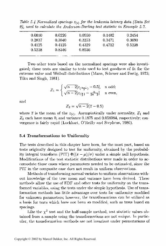
Table 5.4 Normalized spacings z^ for the leukemia latency data (Data Set9), used to calculate the Anderson-Darling test statistic in Example 5.7.

0.00300.28370.41250.5238

0.02260.30400.41250.8346

0.05500.32530.43290.8936

0.14020.34710.4712

0.24540.36900.5238

Two other tests based on the normalized spacings were also investi-gated; these tests are similar to tests used to test goodness of fit for theextreme value and Weibull distributions (Mann, Scheuer and Fertig, 1973;Tiku and Singh, 1981).

{ \/n — 2[z/»-i) — 0.5], n odd;

Vn-2[z(»} - 2^2] n even,

andZ2 = vVi - 2(z - 0.5)

where ~z is the mean of the z^. Asymptotically under normality, Z\ andZ<2 each have mean 0, and variance 0.1875 and 0.056084, respectively; con-vergence is fairly rapid (Lockhart, O'Reilly and Stephens, 1986).

5.4 Transformations to Uniformity

The tests described in this chapter have been, for the most part, based ontests originally designed to test for uniformity, obtained by the probabil-ity integral transform (PIT) <&((x — /^)/cr) under a simple null hypothesis.Modifications of the test statistic distributions were made in order to ac-comodate those cases where parameters needed to be estimated, since thePIT in the composite case does not result in uniform observations.

Methods of transforming normal variates to uniform observations with-out knowledge of the true mean and variance have been derived. Thesemethods allow the use of EDF and other tests for uniformity on the trans-formed variables, using the tests under the simple hypothesis. Use of trans-formation methods has little advantage over tests for uniformity modifiedfor unknown parameters; however, the transformations can be utilized asa basis for tests which have not been so modified, such as tests based onspacings.

Like the %2 test and the half-sample method, test statistic values ob-tained from a sample using the transformations arc not unique. In partic-ular, the transformation methods are not invariant under permutations of


the observations. The values of the transformed variates, and hence of thetest used, are affected by the sequence of observations. Transformation ofnormal variates to uniformity results in n — 2 uniform variates, equivalentto losing two degrees of freedom from parameter estimation.

5.4.1 Characterization of Normality

Characterizing properties of a distribution F are those where a statistict(x\F) has a known distribution if and only if F is true. Csorgo, Seshadriand Yalovsky (1973) presented two transformations of normal variates touniformity based on such a characterization and compare the power of EDFtests using the transformed variates with the Wilk-Shapiro test.

For the first transformation, if a sample Xi,i = 1, . . . ,n are indepen-dent and identically distributed from a normal distribution with unknownmean // and variance cr2, then

n -

are iid normal with mean 0 and variance a1 . From Kotlarski (1966), ifn > 4, and using

V \l]? 7 / / 7 2 I 72 _|_ _i_ 72 J. o „ ojfc — V K / ^ k + i / y ^i T ^2 ' • • • > ^fc' /c — z , . . . , n — z,

then «i = Gi(yi),i = l , . . . , n are independent C/(0,1) random variables,where Gi is the Student's t distribution function with i degrees of freedom.This characterization did not yield goodness of fit tests which had powercomparable to the Wilk-Shapiro test.

A second characterization, useful for odd sample sizes (n = 2fc + 3, k >2), uses the Zj as described above, and defines

Further definefc+i/ _,

andr

r =


Then the r\r act like the order statistics of k independent uniform randomvariables if and only if the x, are normal. This characteriation yieldedEDF tests that were comparable in power to the Wilk-Shapiro test whenthe alternative distribution was symmetric with fa > 3.

5.4.2 The Conditional Probability Integral Transformation

O'Reilly and Quesenberry (1973) discussed the conditional probability inte-gral transformation (CPIT), which is a characterizing transformation whichconditions on sufficient statistics for the unknown parameters in order toobtain f/(0, 1) random variates. Quesenberry (1986) gave the transforma-tion for normal random variables: for a sample from a normal distribution,given complete and sufficient statistics for p and cr2, define Fn(xi, . . . , xn]to be the distribution function of the sample given the statistics. Then then — 2 random variables

are iid U(0, 1) random variables. In particular,

Uj-2 = Gj-2(\(J - l)/t7)(zj - ffj-i)/Sj_i) j = 3 , . . . ,n

are iid uniform random variables, where

k

and

i=l

and Gj is the Student's t distribution function with j degrees of freedom.

5.5 Other Tests for Uniformity

Although the main focus of this text is testing for normality under a com-posite hypothesis, the methods given in the previous section allow the useof simple hypothesis tests when parameters arc unknown.

However, we put less emphasis on these methods because (1) in generalthey seem to result in tests that are less powerful than many tests for


normality given in Chapters 2 through 4 or the composite EDF tests givenin Section 5.1; and (2) they are not invariant under permutations of theobservations. Therefore, we mention only briefly some common goodnessof fit tests used to ascertain the uniformity of a sample. In addition tothose described below, of course, simple EDF tests could be used.

5.5.1 Tests Based on Spacings

The spacings of a sample are defined as the n + I intervals on the hypothe-sized distribution function. Using Stephens (1986a) notation, the spacingsare defined as

with DI = /?(i) and -Dn+i = 1 — P(n)- For uniform jp(j), these spacings areexponentially distributed with mean l/(n + 1). Perhaps the most widelyknown test based on spacings is the Greenwood (1946) test,

n+l

originally introduced as a method of ascertaining whether the incidenceof contagious disease could be described as a Poisson process. Percentagepoints for G are given in Hill (1979), Burrows (1979), Stephens (1981) andCurrie (1981).

Kendall's test (Kendall, 1946; Sherman, 1950) uses the sum of theabsolute differences between the spacings and their expected values,

n+l

Tests based on spacings of ordered uniform takens ra, (ra, > 1) at a timehave also been investigated (e.g., Hartley and Pfaffenberger, 1972; DelPino, 1979; Rao and Kuo, 1984).

5.5.2 Pearson's Probability Product Test

In conjunction with their transformation, one test Csorgo, Seshadri andYalovsky (1973) proposed is Pearson's probability product test (Pearson1933) for testing the uniformity hypothesis. For this test,


which is, under the null hypothesis, a x2 random variable with Ik degreesof freedom.

5.6 Further Reading

D'Agostino and Stephens (1986) contains a number of chapters which covermany of the topics described here in more detail. Stephens (1986a) de-scribes EDF tests, including the case of the simple hypothesis and manynon-normal null distributions. Moore (1986) provides more detail on %2

tests. Stephens (1986b) and Quesenberry (1986) discuss transformationmethods.

References

Anderson, T.W., and Darling, D.A. (1952). Asymptotic theory of cer-tain "goodness of fit" criteria based on stochastic processes. Annals ofMathematical Statistics 23, 193-212.

Anderson, T.W., and Darling, D.A. (1954). A test of goodness of fit.Journal of the American Statistical Association 49, 765-769.

Bishop, Y.M.M., Fienberg, S.E., and Holland, P.W. (1975). DiscreteMultivariate Analysis. MIT Press, Cambridge, Mass.

Braun, H. (1980). A simple method for testing goodness of fit in thepresence of nuisance parameters. Journal of the Royal Statistical SocietyB 42, 53-63.

Burrows, P.M. (1979). Selected percentage points of Greenwood's statistic.Journal of the Royal Statistical Society A 142, 256-258.

Chernoff, H., and Lehmann, E.L. (1954). The use of maximum likelihoodestimates in x2 tests for goodness of fit. Annals of Mathematical Statis-tics 25, 579-586.

Csorgo, M., Seshadri, V., and Yalovsky, M. (1973). Some exact tests fornormality in the presence of unknown parameters. Journal of the RoyalStatistical Society B 35, 507-522.

Currie, I.D. (1981). Further percentage points of Greenwood's statistic.Journal of the Royal Statistical Society A 144, 360-363.

D'Agostino, R.B., and Stephens, M.A. (1986). Goodness of Fit Tech-niques. Marcel Dekker, New York.


David, H.T. (1978). Goodness of fit. In Kruskal, W.H., and Tanur, J.M.,eds., International Encyclopedia of Statistics, The Free Press, NewYork.

David, F.N., and Johnson, N.L. (1948). The probability integral transfor-mation when parameters are estimated from the sample. Biometrika 35,182-192.

Del Pino, G.E. (1979). On the asymptotic distribution of k-spacings withapplications to goodness of fit tests. Annals of Statistics 7, 1058-1065.

Fisher, R.A. (1924). The conditions under which x2 measures the dis-crepancy between observation and hypothesis. Journal of the RoyalStatistical Society 87, 442-450.

Fisher, R.A. (1928). On a property connecting the x2 measure of discrep-ancy with the method of maximum likelihood. Atti Congresso Inter-nazionale dei Mathematici 6, 95-100.

Freeman, M.F., and Tukey, J.W. (1950). Transformations related to theangular and square root. Annals of Mathematical Statistics 21, 607-611.

Green, J.R., and Hegazy, Y.A.S. (1976). Powerful modified EDF goodnessof fit tests. Journal of the American Statistical Association 71, 204-209.

Greenwood, M. (1946). The statistical study of infectious disease. Journalof the Royal Statistical Society A 109, 85-110.

Hartley, H.O., and Pfaffenberger, R.C. (1972). Quadratic forms in orderstatistics used as goodness of fit criteria. Biometrika 59, 605-611.

Hill, I.D. (1979). Approximating the distribution of Greenwood's statisticwith Johnson distributions. Journal of the Royal Statistical Society A142, 378-380.

Kendall, M.G. (1946). Discussion of Professor Greenwood's paper. Journalof the Royal Statistical Society A 109, 103-105.

Kendall, M.G., and Stuart, A. (1973). The Advanced Theory of Statis-tics. Hafner Publishing Co., New York.

Koehler, K.J., and Larntz, K. (1980). An empirical investigation of good-ness of fit statistics for sparse multinomials. Journal of the AmericanStatistical Association 75, 336-444.

Kotlarski, I. (1966). On characterizing the normal distribution by Student'slaw. Biometrika 58, 641-645.

Kuiper, N.H. (1960). Tests concerning random points on a circle. Proceed-ings, Akademie van Wetenschappen A 63, 38-47.


Larntz, K. (1978). Small sample comparisons of exact levels for chi-squaredgoodness of fit statistics. Journal of the American Statistical Association73, 253-263.

Lilliefors, H.W. (1967). On the Kolmogorov-Smirnov test for normalitywith mean and variance unknown. Journal of the American StatisticalAssociation 62, 399-402.

Lockhart, R.A., O'Reilly, F.J., and Stephens, M.A. (1986). Tests of fitbased on normalized spacings. Journal of the Royal Statistical SocietyB 48, 344-352.

Mann, N.R., Scheuer, E.M., and Fcrtig, K.W. (1973). A new goodness offit test for the two parameter Weibull or extreme value distribution withunknown parameters. Communications in Statistics 2, 838-900.

Mann, H.B., and Wald, A. (1942). On the choice of the number of inter-valsin the application of the chi-square test. Annals of MathematicalStatistics 13, 306-317.

Moore, D.S. (1986). Tests of chi-squared type. In D'Agostino, R.B, andStephens, M.A., cds., Goodness of Fit Techniques, Marcel Dekker,New York.

Neyrnan, J. (1937). 'Smooth test' for goodness of fit. Skandinaviske Aktu-arietiddkrift 20, 150-199.

Neyman, J. (1949). Contributions to the theory of the x2 test. In Pro-ceedings of the First Berkeley Symposium on MathematicalStatistics and Probability, University of California Press, 239-273.

O'Reilly, F.J., and Quesenberry, C.P. (1973). The conditional probabilityintegral transformation and applications to obtain composite chi-squaregoodness of fit tests. Annals of Statistics 1, 74-83.

Pearson, K. (1900). On the criterion that a given system of deviations fromthe probable in the case of a correlated system of variables is such thatit can be reasonably supposed to have arisen from random sampling.Philosophical Magazine 50, 157-175.

Pearson, K. (1933). On a method of determining whether a sample of size nsupposed to have been drawn from a parent population having a knownprobability integral has probably been drawn at random. Biometrika25, 379-410.

Quesenberry, C.P. (1986). Some transformation methods in goodenss offit. In D'Agostino, R.B, and Stephens, M.A., eds., Goodness of FitTechniques, Marcel Dekker, New York.


Rao, J.S., and Kuo, M. (1984). Asymptotic results on the Greenwoodstatistic and some of its generalizations. Journal of the Royal StatisticalSociety B 46, 228-237.

Shapiro, S.S., and Wilk, M.B. (1965). An analysis of variance test fornormality (complete samples). Biometrika 52, 591-611.

Sherman (1950). A random variable related to the spacings of samplevalues. Annals of Mathematical Statistics 21, 339-361.

Stephens, M.A. (1974). EDF statistics for goodness of fit and some com-parisons. Journal of the American Statistical Association 69, 730-737.

Stephens, M.A. (1978). On the half-sample method for goodness of fit.Journal of the Royal Statistical Society B 40, 64-70.

Stephens. M.A. (1981). Further percentage points for Greenwood's statis-tic. Journal of the Royal Statistical Society A 144, 364-366.

Stephens, M.A. (1986a). Tests based on EDF Statistics. In D'Agostinoand Stephens, eds., Goodness of Fit Techniques, Marcel Dekker,New York.

Stephens, M.A. (1986b). Tests for the uniform distribution. In D'Agostinoand Stephens, eds., Goodness of Fit Techniques, Marcel Dekker,New York.

Thomas, D.R., and Pierce, D.A. (1979). Neyman's smooth goodness offit test when the hypothesis is composite. Journal of the AmericanStatistical Association 74, 441-445.

Tiku, M.L., and Singh, M. (1981). Testing for the two parameter Weibulldistribution. Communications in Statistics - Theory and Methods 10,907-918.

Watson, G.S. (1961). Goodness of fit tests on a circle. Biometrika 48,109-114.

Watson, G.S. (1962). Goodness of fit tests on a circle. II. Biometrika 49,57-63.


6goodness of fit tests

Documents

range of tests

mises tests

powerful tests

tests specific

tests areunique

hypothesized null distribution

distribution offox0

thenull distribution