Power Flow Analysis on CUDA-based GPU

by

Yizheng Liao

A Major Qualifying Project Report

Submitted to the Faculty

of the

WORCESTER POLYTECHNIC INSTITUTE

in partial fulfillment of the requirements for the

Degree of Bachelor of Science

in

Electrical and Computer Engineering

by

May 2011

APPROVED:

Professor Xinming Huang, MQP Advisor

Abstract

This major qualifying project investigates the algorithm and the performance of using the

CUDA-based Graphics Processing Unit for power flow analysis. The accomplished work

includes the design, implementation and testing of the power flow solver. Comprehensive

analysis shows that the execution time of the parallel algorithm outperforms that of the

sequential algorithm by several factors.

iii

Acknowledgements

I would like to express my deep and sincere gratitude to my academic and MQP advisor,

Professor Xinming Huang, for giving me the professional and insightful comments and

suggestions on this project.

iv

Contents

List of Figures v

List of Tables vi

1 Introduction 1

2 Background 3

2.1 Power Flow Model . . . . . . . . . . . . . . . . . . . . . . . . . . . . . . . . 32.1.1 Branches . . . . . . . . . . . . . . . . . . . . . . . . . . . . . . . . . 42.1.2 Generators . . . . . . . . . . . . . . . . . . . . . . . . . . . . . . . . 62.1.3 Loads . . . . . . . . . . . . . . . . . . . . . . . . . . . . . . . . . . . 62.1.4 Shunt Elements . . . . . . . . . . . . . . . . . . . . . . . . . . . . . . 62.1.5 Transmission System . . . . . . . . . . . . . . . . . . . . . . . . . . . 7

2.2 Power Flow Analysis . . . . . . . . . . . . . . . . . . . . . . . . . . . . . . . 82.2.1 Solving Power Flow Problem . . . . . . . . . . . . . . . . . . . . . . 9

2.3 Gauss-Jacobi Iterative Method . . . . . . . . . . . . . . . . . . . . . . . . . 112.4 CUDA Overview . . . . . . . . . . . . . . . . . . . . . . . . . . . . . . . . . 14

3 Algorithm and Implementation 18

3.1 Data Structure . . . . . . . . . . . . . . . . . . . . . . . . . . . . . . . . . . 183.2 Building Bus Admittance Matrix . . . . . . . . . . . . . . . . . . . . . . . . 203.3 Solving Power Flow Problem . . . . . . . . . . . . . . . . . . . . . . . . . . 27

4 Performance Analysis 32

5 Conclusion 35

A NVIDIA GeForce GTS 250 GPU 36

Bibliography 37

v

List of Figures

2.1 Branch Model . . . . . . . . . . . . . . . . . . . . . . . . . . . . . . . . . . . 42.2 Grid of Thread Blocks [1] . . . . . . . . . . . . . . . . . . . . . . . . . . . . 152.3 Overview of CUDA device memory model [2] . . . . . . . . . . . . . . . . . 16

4.1 Execution time for CUDA-based power flow solver and MATPOWER powerflow solver . . . . . . . . . . . . . . . . . . . . . . . . . . . . . . . . . . . . . 33

vi

List of Tables

2.1 CUDA Memory Type . . . . . . . . . . . . . . . . . . . . . . . . . . . . . . 16

3.1 Bus Data . . . . . . . . . . . . . . . . . . . . . . . . . . . . . . . . . . . . . 183.2 Generator Data . . . . . . . . . . . . . . . . . . . . . . . . . . . . . . . . . . 193.3 Branch Data . . . . . . . . . . . . . . . . . . . . . . . . . . . . . . . . . . . 20

4.1 Execution time for power flow solver . . . . . . . . . . . . . . . . . . . . . . 32

A.1 NVIDIA GeForce GTS 250 GPU Specification . . . . . . . . . . . . . . . . . 36

1

Chapter 1

Introduction

The smart grid has been discussed widely in both academic and industry. Many research

and development projects have pointed out the functionalities of the smart grid [3]:

• Self-healing

• High reliability and power quality

• Accommodates a wide variety of distributed generation and storage options

• Optimizes asset utilization

• Minimizes operations and maintenance expenses

In order to realize these functions, each unit of the power system, such as the power

plant, the grid operator, and the customer, needs to know the on-line power flow. For

example, a power plant wants to change its output based on the total power consumption

of a city. In order to achieve it, the power plant needs to collect the grida data and compute

the power consumption. This is called the power flow analysis.

The power flow analysis has been widely developed since 1960s [4]. Many algorithms

have been proposed on this area. However, in the case we presented above, we assume

there are at least ten thousands buses in the city-scale grid. Consequently, the computation

of the power consumption has a high latency, which may delay the power plant decision.

2

Therefore, a fast way to compute the grid information is necessary. One approach is using

the parallel computation to solve it.

Nowadays, the hardware device has been widely used for high performance computation.

The most well known devices include the multi-core CPU, the Field-programmable Gate

Array (FPGA), and the Graphic Processing Unit (GPU). The multi-core CPU has very high

clock frequency. However, compared with FPGA and GPU, the number of thread on GPU

is limited. An FPGA is a custom integrated circuit that generally includes a large number

of logical cells [5]. Each logical cell is available for handling a single task from a predefined

set of functions. However, the drawback for using FPGA for power flow problem is the

computation of floating point on FPGA is not efficient. Similar to the FPGA, the each

thread on the GPU can handle a single task based the predefined function. In addition, the

recent released CUDA GPU, which is developed by NVIDIA, is available for programming

by C, which is more convenient than the hardware language, such as VHDL. In addition,

among these three devices, the GPU can be purchased by a very cheap price.

In this project, we investigate the algorithm for using CUDA-based GPU to solve the

problem flow problem. Also, we use the developed algorithm to test the IEEE power flow

test case. The execution time is compared with the Matlab-based power flow solver, which

solves the problem in a sequential way. The performance analysis shows that the execution

time of the parallel algorithm is much faster than the sequential algorithm.

3

Chapter 2

Background

2.1 Power Flow Model

In order to analysis the transmission system, we need to model the buses or nodes

interconnected by transmissions links. Generators and loads, which are connected to various

buses in the system, inject and remove power from the transmission system. As discussed

in [6], we assume that each transmission link is represented by a per phase Π-equivalent

circuit. Then for each bus i, the relationship between the complex voltage Vi and the

complex current Ii is

Ii = Y × Vi. (2.1)

If we extend (2.1) to all the buses, for a n buses system, we can use nodal analysis to relate

all the bus currents to the bus voltage. In matrix notation, this relationship is

I = YbusV (2.2)

where

I =

I1

I2...

In

(2.3)

4

and

V =

V1

V2

...

Vn

. (2.4)

In (2.2), the n× n matrix Ybus is called the bus admittance matrix. Its element is equal to

[6]

• yii =∑

admittances of Π-equivalent circuit elements incident to the ith bus

• yik = − admittance of Π-equivalent circuit elements bridging the ith and kth buses

In this project, we created Ybus by the method given in [7].

2.1.1 Branches

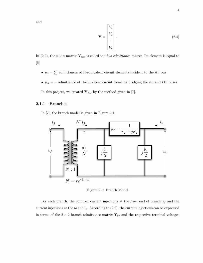
In [7], the branch model is given in Figure 2.1.

Figure 2.1: Branch Model

For each branch, the complex current injections at the from end of branch if and the

current injections at the to end it. According to (2.2), the current injections can be expressed

in terms of the 2 × 2 branch admittance matrix Ybr and the respective terminal voltages

5

vf and vt,

if

it

= Ybr

vf

vt

(2.5)

In (2.5), the branch admittance matrix Ybr can be written as

Ybr =

(ys + j bc2 )

1τ2

−ys1

τ exp(−jθshift)

−ys1

τ exp(jθshift)ys + j bc

2

(2.6)

where

• ys = 1/zs denotes the series admittance and zs = rs + jxs is the series impedance in

Π transmission line model

• bc denotes the total charging capacitance

• τ denotes the magnitude of the transformer tap ratio

• θshift denotes the phase shift angle of the transformer tap ratio.

For branch i, if the four elements of Yibr is labelled as shown in (2.7)

Yibr =

yiff yift

yitf yitt

, (2.7)

therefore, for a transmission system with nl lines,

Ybr =

Yff Yft

Ytf Ytt

(2.8)

where each element is a nl × 1 vector and the ith element of each vector comes from the

corresponding element of Ybr.

In addition, the connection matrices Cf and Ct are used to build the system admittance

matrices Ybus as well. For each branch i connects from bus j to bus k, the (i, j) element

of Cf and the (i, k) element of Ct are equal to one. All other elements are zero. For a nb

buses transmission system with nl branches, the demission of Cf and Ct is nl × nb.

6

2.1.2 Generators

A generator is connected to a specific bus as the complex power injection. For generator

i, the power injection is

sig = pig + jqig. (2.9)

Therefore, for a system with ng generators, (2.9) can be expressed in a vector form,

Sg = Pg + jQg (2.10)

where Sg, Pg, and Qg are ng × 1 vectors.

In order to map the generator to the bus, we build the nb × ng generator connection

matrix Cg. When generator j is located at bus i, the (i, j) element of Cg is one. Other

elements are zero.

2.1.3 Loads

A load bus is modelled as a complex consumption at a specific bus. For bus i, the load

is

sid = pid + jqid. (2.11)

Hence, for a system with nb buses, (2.11) becomes to

Sd = Pd + jQd (2.12)

where Sd, Pd, and Qd are nb × 1 vectors.

2.1.4 Shunt Elements

Both capacitor and inductor are called shunt connected element. A shunt element is

modelled as a fixed impedance connected to ground at a bus. For bus i, the admittance of

the shunt element is given as

yish = gish + jbish. (2.13)

7

Thus, for a system with nb buses, (2.13) is expressed as

Ysh = Gsh + jBsh (2.14)

where Ysh, Gsh, and Bsh are nb × 1 vectors.

2.1.5 Transmission System

Recall the transmission equation (2.2). For a system with nb buses, all impedance

elements of the model are included in a nb × nb complex matrix Ybus, which relates the

complex node current injections Ibus and the complex node voltage V.

The similar idea applies to the branch system. For a system with nl branches, the nl×nb

branch admittance matrices Yf and Yt relate the bus voltages to the branch currents If

and It at the from and to ends of all branches, as shown in (2.15) and (2.16).

If = YfV (2.15)

It = YtV (2.16)

The admittance matrices can be computed as

Yf = [Yff ]Cf + [Yft]Ct, (2.17)

Yt = [Ytf ]Cf + [Ytt]Ct, (2.18)

and

Ybus = CTf Yf +CT

t Yt + [Ysh] (2.19)

where [.] denotes an operator that takes an n×1 vector and creates a n×n diagonal matrix

with the vector elements on the diagonal, and T denotes the matrix transpose.

The complex power injections now can be computed as functions of the complex bus

voltages V as

Sbus(V) = [V]I∗bus = [V]Y∗busV

∗, (2.20)

8

Sf (V) = [CfV]I∗f = [CfV]Y∗fV

∗, (2.21)

and

St(V) = [CtV]I∗t = [CtV]Y∗tV

∗ (2.22)

where ∗ denotes the complex conjugate of each element.

For a AC power model, the total power should balance. Therefore, we have the system

power function:

gs(V,Sg) = Sbus(V) + Sd −CgSg = 0. (2.23)

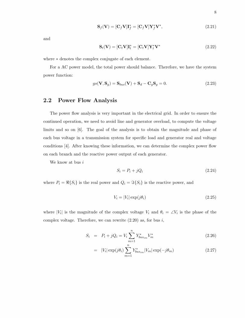
2.2 Power Flow Analysis

The power flow analysis is very important in the electrical grid. In order to ensure the

continued operation, we need to avoid line and generator overload, to compute the voltage

limits and so on [6]. The goal of the analysis is to obtain the magnitude and phase of

each bus voltage in a transmission system for specific load and generator real and voltage

conditions [4]. After knowing these information, we can determine the complex power flow

on each branch and the reactive power output of each generator.

We know at bus i

Si = Pi + jQi (2.24)

where Pi = <{Si} is the real power and Qi = ={Si} is the reactive power, and

Vi = |Vi| exp(jθi) (2.25)

where |Vi| is the magnitude of the complex voltage Vi and θi = ∠Vi is the phase of the

complex voltage. Therefore, we can rewrite (2.20) as, for bus i,

Si = Pi + jQi = Vi

n∑

m=1

Y ∗busim

V ∗m (2.26)

= |Vi| exp(jθi)

n∑

m=1

Y ∗busim

|Vm| exp(−jθm) (2.27)

9

In (2.26), we have four variables, Pi, Qi, |Vi|, and θi. The solution to the power flow

problem begins with identifying if each variable of these four are known in the system. In

fact, the known and unknown variables depend on the type of bus. In the transmission

system, we have three types of bus:

• Load bus: a bus without any generators connected to it

• Generator bus: a bus has at least one generator connected to it

• Slack bus: a reference generator bus

For each type of bus, two out of four variables are known. For load bus, we assume

Pi = −P id and Qi = −Qi

d are known. In power flow problem, the load bus is usually called

as PQ bus. For generator bus, we assume Pi = P ig −P i

d and |Vi| are known. The generator

bus is usually called as PV bus in power flow system. For the slack bus, we assume |Vi|

and θi are known. Therefore, for each PQ bus, we must solve for |Vi| and θi. For each PV

bus, we must solve for θi. For slave bus, none of the variables must be solved. For each

bus, after solving |Vi| and θi, we can compute Pi and Qi by (2.26).

2.2.1 Solving Power Flow Problem

As discussed above, the key to solve the power flow problem is finding the complex

voltage of each bus. After that, we can easily find the complex power of each bus. In power

flow problem, there are two cases of problem. The first case knows V1, S2, S3, . . . , Sn and

solves S1, V2, V3, . . . , Vn.

For (2.26), we assume i = 1 is the slack bus. We can separate it from other buses.

Hence, we rewrite (2.26) as

S1 = V1

n∑

m=1

Y ∗bus1m

V ∗m (2.28)

Si = Vi

n∑

m=1

Y ∗busim

V ∗m i = 2, 3, . . . , n (2.29)

In (2.28), it we know V1, V2, . . . , Vn, we can solve for S1 explicitly by using (2.28). Since bus

1 is the slack bus, we have known V1. Therefore, we only need to find V2, . . . , Vn. These

10

n− 1 unknowns can be found by using (2.29). Hence, the key for solving case I problem is

finding the solution of n− 1 implicit equations in the unknown V2, V3, . . . , Vn, where V1 and

S2, S3, . . . , Sn are known.

Now let’s take complex conjugates of (2.29). Then we have

S∗i = V ∗

i

n∑

m=1

YbusimVm i = 2, 3, . . . , n (2.30)

Dividing (2.28) by V ∗i and separating the Ybusii term, we can rewrite (2.28)

S∗i

V ∗i

=

n∑

m=1

YbusimVm (2.31)

S∗i

V ∗i

= YbusiiVi +

n∑

m=1,m6=i

YbusimVm i = 2, 3, . . . , n (2.32)

or, equivalently,

Vi =1

Ybusii

S∗i

V ∗i

−n∑

m=1,m6=i

YbusimVm

i = 2, 3, . . . , n (2.33)

Thus, now we have a non-linear system which can be solved by using the iteration method,

such as the Jacobi method or Gauss-Seidel method. We can rewrite (2.33) in the iterative

form, which is shown in (2.34).

V(k)i =

1

Ybusii

S∗i

V∗(k−1)i

−

n∑

m=1,m6=i

YbusimV(k−1)m

i = 2, 3, . . . , n (2.34)

The second case of the power flow problem knows V1, (P2, |V2|), . . . , (Pl, |Vl|), Sl+1, . . . , Sn.

The unknown variables are S1, (Q2, θ2), . . . , (Ql, θl), Vl+1, . . . , Vn. In this case, for the slack

bus, we can use (2.28) to find S1 after solving all the variables of other buses. For other

buses, the procedure is similar to the case I.

In case II, we have both PQ buses and PV buses. For PQ buses, since we have known

11

Pi and Qi, we can use (2.34) to compute Vi. Therefore, we have the iterative formula:

V(k)i =

1

Ybusii

S∗i

V∗(k−1)i

−

n∑

m=1,m6=i

YbusimV(k−1)m

i = l + 1, l + 2, . . . , n (2.35)

For PV buses, although Qi is unknown, we can perform a side calculation to estimate

it on the basis of the kth step voltage. Thus, by using (2.29), we have

Qi = =

[

V(k)i

n∑

m=1

Ybus∗im(V (k)

m )∗

]

i = 2, 3, . . . , l (2.36)

Then, we can compute the complex voltage for PV buses by using (2.37).

V(k)i =

1

Ybusii

S∗i

V∗(k−1)i

−

n∑

m=1,m6=i

YbusimV(k−1)m

i = 2, 3, . . . , l (2.37)

2.3 Gauss-Jacobi Iterative Method

Gauss-Jacobi iterative method, usually refers to Jacobi method, is an algorithm for

finding the solutions of a linear equations system.

Suppose a system of n linear equations is given. Each equation contains n variables.

Therefore, we have

a11x1 + a12x2 + . . . a1nxn = b1

a21x1 + a22x2 + . . . a2nxn = b2...

an1x1 + an2x2 + . . . annxn = bn

(2.38)

We can write the linear equations in (2.38) into a matrix form. Then we have

Ax = b (2.39)

12

where

A =

a11 a12 · · · a1n

a21 a22 · · · a2n...

.... . .

...

an1 an2 · · · ann

, (2.40)

x =

x1

x2...

xn

, (2.41)

and

b =

b1

b2...

bn

(2.42)

We can re-write the matrix A in a form of

A = D+R (2.43)

where

D =

a11 0 · · · 0

0 a22 · · · 0...

.... . .

...

0 0 · · · ann

(2.44)

and

R =

0 a12 · · · a1n

a21 0 · · · a2n...

.... . .

...

an1 an2 · · · 0

. (2.45)

13

Now, we can re-write the linear system (2.40) as

(D+R)x = b

Dx+Rx = b

Dx = b−Rx

x = D−1(b−Rx). (2.46)

The Jacobi method is an iterative method that solves the linear system in (2.46). (2.46)

can be written in an iterative form as

x(k+1) = D−1(b−Rxk). (2.47)

where k is the iterative index.

Since the matrix D is a diagonal matrix, we can easily compute D−1, as shown in (2.48)

D−1 =

1a11

0 · · · 0

0 1a22

· · · 0...

.... . .

...

0 0 · · · 1ann

(2.48)

Therefore, the element-based formula for the Jacobi method is [8]

x(k+1)i =

1

aii

bi −

j=n∑

j=1,j 6=i

aijx(k)j

, i = 1, 2, . . . , n. (2.49)

The stopping criteria for the Jacobi method includes two conditions:

1. ||x(k)−x(k−1)||∞ ≤ ε, where ||.||∞ denotes the infinity norm and ε is the error tolerance

2. k = K, where K denotes the maximum number of iteration.

When either of them is satisfied, the iteration will stop and output the latest xk as the

solution of the linear system (2.39).

The algorithm of the Jacobi method is described in Algorithm 1.

14

Algorithm 1 Jacobi Method

Import A,b,x(0)

φ = 1, k = 0while φ ≥ ε do

k = k + 1for i = 1 → n do

τ = 0for (j = 1 → n) AND j 6= i do

τ = τ + aijx(k−1)j

end for

x(k)i = bi−τ

aiiend for

if (k + 1) == K then

BREAKend if

φ = max{|x(k)1 − x

(k−1)1 |, |x

(k)2 − x

(k−1)2 |, . . . , |x

(k)n − x

(k−1)n |}

end while

2.4 CUDA Overview

Graphic Processing Unit (GPU) is a high performance computing device. Due to its

architecture, the number of cores of GPU exceeds that of multi-core CPUS greatly. There

are hundreds of cores in mainstream GPUs, therefore, the parallel computation capacity of

GPU is much higher than that of multi-core CPU.

CUDA, stands for Compute Unified Device Architecture, is a new computing architec-

ture for GPU, which is introduced by NVIDIA Corporation in 2006 [9]. Compared with

the previous GPU architecture, the CUDA GPU provides a more convenient tool for the

developers to perform large scale parallel computation via GPU [10].

In this project, we use NVIDIA GeForce GTS 250 CUDA GPU to run the simulation.

There are 16 SMs (Streaming Multiprocessors), with 8 scalar processors in each SM. Thus,

in total, there are 128 cores in GreForce GTS 250. When a parallel task is launched, the

task will be implemented by a function called kernel function, which is run by one thread.

These threads are first grouped into blocks and then blocks are organized by one grid.

This relationship is shown in Figure 2.2. Threads in the same block are separated into a

scheduling unit called warp. On the GPU we used, each warp contains 32 threads. More

details are given in Appendix A.

15

Figure 2.2: Grid of Thread Blocks [1]

16

In CUDA GPU, there are five types of memory. The following table provides the details

about the memory type, the range of threads that can access the memory, which is called

scope, and the lifetime, which specifies the lifetime of the variable defined in different type

of memory [2]. Figure 2.3 shows the memory model.

Table 2.1: CUDA Memory Type

Memory Scope Lifetime

Register Thread Kernel

Local Thread Kernel

Shared Block Kernel

Global Grid Application

Constant Grid Application

Figure 2.3: Overview of CUDA device memory model [2]

In these memories, the register has the fastest access speed. Each thread is assigned

several registers and the assigned register can only be called by its master thread. However,

17

in CUDA, the number of available registers are limited. On GeForce GTS 250, the available

registers for each block is 8192. Therefore, if we launch 512 threads in each block, then

each thread is only assigned 16 registers. Therefore, we need to plan ahead to ensure all

the available registers are used effectively.

In each block, the shared memory can be accessed by all the threads within the block.

In CUDA programming, the shared memory is frequently used to read data from the global

memory and then share the data among the threads [11]. However, the available space of

the shared memory is a concern. Only 16384 bytes are available for each block. Usually,

we store the frequently used data in shared memory.

The global memory has the largest space among all the types of memory. On GeForce

GTS 250, the available global memory is about 500 MB. However, the access to the global

memory from thread is not efficient. Also, each thread accesses the global memory in a

sequential way. Therefore, in CUDA programming, we try to minimize the access from the

threads to the global memory.

On CUDA GPU, all the readable data and variables for each thread is stored on the

device memory. In CUDA, the bandwidth of the communication between the host, which

refers to the PC, and the device, which refers to the GPU, is much lower than the bandwidth

of the communication between devices. Therefore, we try to transfer all the necessary data

for computation from the host to the device.

18

Chapter 3

Algorithm and Implementation

This chapter, we will provide detailed study for how to use GPU to solve problem flow

problem in parallel.

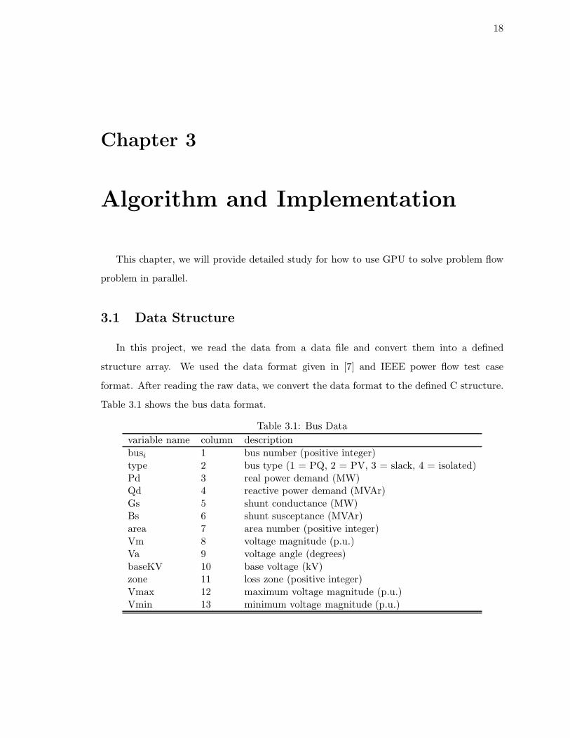
3.1 Data Structure

In this project, we read the data from a data file and convert them into a defined

structure array. We used the data format given in [7] and IEEE power flow test case

format. After reading the raw data, we convert the data format to the defined C structure.

Table 3.1 shows the bus data format.

Table 3.1: Bus Data

variable name column description

busi 1 bus number (positive integer)type 2 bus type (1 = PQ, 2 = PV, 3 = slack, 4 = isolated)Pd 3 real power demand (MW)Qd 4 reactive power demand (MVAr)Gs 5 shunt conductance (MW)Bs 6 shunt susceptance (MVAr)area 7 area number (positive integer)Vm 8 voltage magnitude (p.u.)Va 9 voltage angle (degrees)baseKV 10 base voltage (kV)zone 11 loss zone (positive integer)Vmax 12 maximum voltage magnitude (p.u.)Vmin 13 minimum voltage magnitude (p.u.)

19

Table 3.2 shows the data format of generators.

Table 3.2: Generator Data

variable name column description

busi 1 bus number (positive integer)Pg 2 real power output (MW)Qg 3 reactive power output (MVAr)Qmax 4 maximum reactive power output (MVAr)Qmin 5 minimum reactive power output (MVAr)Vg 6 voltage magnitude setpoint (p.u.)mBase 7 total MVA base of machine, defaults to baseMVAstatus 8 machine status, if it is positive, then machine in servicePmax 9 maximum real power output (MW)Pmin 10 minimum real power output (MW)Pc1 11 lower real power output of PQ capability curve (MW)Pc2 12 upper real power output of PQ capability curve (MW)Qc1min 13 minimum reatice power output at PC1 (MVAr)Qc1max 14 maximum reatice power output at PC1 (MVAr)Qc2min 15 minimum reatice power output at PC2 (MVAr)Qc2max 16 maximum reatice power output at PC2 (MVAr)rampagc 17 ramp rate for load following/AGC (MW/min)

ramp10 18 ramp rate for 10 minute reserves (MW)ramp30 19 ramp rate for 30 minute reserves (MW)rampq 20 ramp rate for reactive power (2 sec time-scale) (MVAr/min)

apf 21 area participation factor

Table 3.3 shows the data format of branches.

20

Table 3.3: Branch Data

variable name column description

fbus 1 “from” bus numbertbus 2 “to” bus numberr 3 resistance (p.u.)x 4 reactance (p.u.)b 5 total line charging susceptance (p.u.)rateA 6 MVA rating A (long term rating)rateB 7 MVA rating B (short term rating)rateC 8 MVA rating C (emergency rating)ratio 9 transformer off nominal turns ratio,

(taps at “from” bus, impedance at “to” bus)angle 10 transformer phase shift angle (degrees), positive → delaystatus 11 initial branch state, 1 = in-service, 0 = out-of-serviceangmin 12 minimum angle difference, θf − θt (degree)angmax 13 maximum angle difference, θf − θt (degree)PF 14 real power injected at “from” bus end (MW)QF 15 reactive power injected at “from” bus end (MVAr)PT 16 real power injected at “to” bus end (MW)QT 17 reactive power injected at “to” bus end (MVAr)

3.2 Building Bus Admittance Matrix

In order to build the bus admittance matrix Ybus, we follow the equations given in

section 2.1. For each element of Ybus, the data type is cuFloatComplex, where is a single-

precision complex number defined by CUDA library. The following part of this section

shows how we construct Ybus.

Firstly, we construct the branch admittance matrix Ybr and the associated elements

Yff ,Yft,Ytf , and Ytt. We use the matrix (2.6) to build each element. Here is the C code

for doing this step:

1 for (unsigned int i = 1 ; i <= branch s i z e ; i++)

2 {

3 State = make cuFloatComplex ( ( br [ IDX1F( i ) ] . s t a tu s ) , ( 0 . 0 f ) ) ;

4 Ys . e lements [ IDX1F( i ) ] =

5 cuCdivf ( State ,

6 make cuFloatComplex ( ( br [ IDX1F( i ) ] . r ) ,

21

7 ( br [ IDX1F( i ) ] . x ) ) ) ;

8

9 Bc . e lements [ IDX1F( i ) ] =

10 cuCmulf ( State ,

11 make cuFloatComplex ( ( br [ IDX1F( i ) ] . b ) , ( 0 . 0 f ) ) ) ;

12

13 i f ( br [ IDX1F( i ) ] . r a t i o != 0)

14 {

15 tap . e lements [ IDX1F( i ) ] =

16 make cuFloatComplex ( ( br [ IDX1F( i ) ] . r a t i o ) ,

17 ( 0 . 0 f ) ) ;

18 }

19 else

20 {

21 tap . e lements [ IDX1F( i ) ] =

22 make cuFloatComplex ( 1 , ( 0 . 0 f ) ) ;

23 }

24 theta = 180/ p i ∗br [ IDX1F( i ) ] . ang le ;

25

26 tap . e lements [ IDX1F( i ) ] =

27 cuCmulf ( ( tap . e lements [ IDX1F( i ) ] ) ,

28 make cuFloatComplex ( ( ( f loat ) cos ( theta ) ) ,

29 ( ( f loat ) s i n ( theta ) ) ) ) ;

30

31

32 Ytt . e lements [ IDX1F( i ) ] =

33 cuCaddf (Ys . e lements [ IDX1F( i ) ] ,

34 make cuFloatComplex ( ( 0 . 0 f ) ,

35 ( cuCrea l f (Bc . e lements [ IDX1F( i ) ] ) / 2 ) ) ) ;

22

36

37 Yff . e lements [ IDX1F( i ) ] =

38 cuCdivf ( Ytt . e lements [ IDX1F( i ) ] ,

39 cuCmulf ( tap . e lements [ IDX1F( i ) ] , tap . e lements [ IDX1F( i ) ] ) ) ;

40

41 Ys . e lements [ IDX1F( i ) ] =

42 make cuFloatComplex ((−1∗ cuCrea l f (Ys . e lements [ IDX1F( i ) ] ) ) ,

43 (−1∗cuCimagf (Ys . e lements [ IDX1F( i ) ] ) ) ) ;

44

45 Yft . e lements [ IDX1F( i ) ] =

46 cuCdivf (Ys . e lements [ IDX1F( i ) ] ,

47 cuConjf ( tap . e lements [ IDX1F( i ) ] ) ) ;

48

49 Ytf . e lements [ IDX1F( i ) ] =

50 cuCdivf (Ys . e lements [ IDX1F( i ) ] ,

51 tap . e lements [ IDX1F( i ) ] ) ;

52

53 }

Then we build the shunt admittance Ysh by using (2.13). Here is the C code:

1 for (unsigned int i = 1 ; i <= bus s i z e ; i++)

2 {

3 Ysh . e lements [ IDX1F( i ) ] =

4 make cuFloatComplex ( ( bus [ IDX1F( i ) ] . Gs/baseMVA) ,

5 ( bus [ IDX1F( i ) ] . Bs/baseMVA) ) ;

6 }

Before implementing (2.17), (2.18) and (2.19), we need to build the branch connection

matrix. This listing shows how we build the connection matrix:

1 for (unsigned int i = 1 ; i <= branch s i z e ; i++)

2 {

23

3 unsigned int j = br [ IDX1F( i ) ] . fbus ;

4 unsigned int k = br [ IDX1F( i ) ] . tbus ;

5

6 Cf . e lements [ IDX2F( i , j , b r anch s i z e ) ] =

7 make cuFloatComplex ( ( 1 . 0 f ) , ( 0 . 0 f ) ) ;

8 Ct . e lements [ IDX2F( i , k , b ranch s i z e ) ] =

9 make cuFloatComplex ( ( 1 . 0 f ) , ( 0 . 0 f ) ) ;

10 }

Now, we have enough for building Ybus by using (2.17), (2.18) and (2.19). Since in

this project, we consider a situation that there are thousands buses in the system. It is

not efficient to compute Yf , Yt and Ybus in a sequence way because a large amount of

computation is required. For each element of Yf or Yt, 2nb complex multiplications and

2nb complex additions are needed, where nb is the number of buses. Therefore, we use the

GPU to build Yf and Yt. Each thread computes the value of one element in Yf and Yt.

Here is the kernel function:

1 g l o b a l void MakeYfYt ( const cVector Y1 , const cVector Y2 ,

2 const cMatrix Cf , const cMatrix Ct , cMatrix Y)

3 {

4 const unsigned int tx = threadIdx . x+1;

5 cuFloatComplex temp1 ;

6 s h a r e d cuComplex C0 ;

7 C0 = make cuFloatComplex ( ( 0 . 0 f ) , ( 0 . 0 f ) ) ;

8 s yn c th r ead s ( ) ;

9

10

11 for (unsigned int j = 1 ; j <= Y. width ; j++)

12 {

13 Y. elements [ IDX2F( tx , j ,Y. he ight ) ] = C0 ;

14 temp1 = cuCmulf (Y1 . e lements [ IDX1F( tx ) ] ,

24

15 Cf . e lements [ IDX2F( tx , j , Cf . he ight ) ] ) ;

16

17 Y. elements [ IDX2F( tx , j ,Y. he ight ) ] =

18 cuCaddf (Y. elements [ IDX2F( tx , j ,Y. he ight ) ] ,

19 temp1 ) ;

20

21 temp1 = cuCmulf (Y2 . e lements [ IDX1F( tx ) ] ,

22 Ct . e lements [ IDX2F( tx , j , Ct . he ight ) ] ) ;

23 Y. elements [ IDX2F( tx , j ,Y. he ight ) ] =

24 cuCaddf (Y. elements [ IDX2F( tx , j ,Y. he ight ) ] ,

25 temp1 ) ;

26

27 }

28

29 syn c th r ead s ( ) ;

30

31 }

For this kernel function, the dimension of the block is nl × 1, where nl is the number of

buses, and the dimension of the grid is 1×1. Here we show how we call the kernel function:

1 dim3 dimBlockYtYf (YDevice . Yf . height , 1 ) ;

2 dim3 dimGridYtYf ( 1 , 1 ) ;

3

4

5 //Yf

6 MakeYfYt<<<dimGridYtYf , dimBlockYtYf>>>

7 ( YffDevice , YftDevice , CfDevice , CtDevice , YDevice . Yf ) ;

8 CheckCUDAKernalError ( ”Computer Yf” ) ;

9

10

25

11 //Yt

12 MakeYfYt<<<dimGridYtYf , dimBlockYtYf>>>

13 ( YtfDevice , YttDevice , CfDevice , CtDevice , YDevice . Yt ) ;

14 CheckCUDAKernalError ( ”Computer Yt” ) ;

For Ybus, we use kernel function to build it as well. Here is the kernel function:

1 g l o b a l void MakeYbus( const cMatrix Cf , const cMatrix Ct ,

2 const cMatrix Yf , const cMatrix Yt ,

3 const cVector Ysh , cMatrix Ybus)

4 {

5 const int tx = blockIdx . x ∗ blockDim . x + threadIdx . x+1;

6 // const i n t t y = b l o c k I dx . y ∗ blockDim . y + threadIdx . y+1;

7 cuFloatComplex temp1 , temp2 , temp3 ;

8

9 for (unsigned int ty = 1 ; ty <= Ybus . width ; ty++)

10 {

11

12

13 temp1 = make cuFloatComplex ( ( 0 . 0 f ) , ( 0 . 0 f ) ) ;

14 temp2 = make cuFloatComplex ( ( 0 . 0 f ) , ( 0 . 0 f ) ) ;

15 temp3 = make cuFloatComplex ( ( 0 . 0 f ) , ( 0 . 0 f ) ) ;

16 // temp4 = make cuFloatComplex ( ( 0 . 0 f ) , ( 0 . 0 f ) ) ;

17

18 for (unsigned int k = 1 ; k <= Yf . he ight ; k++)

19 {

20 temp3 = cuCmulf (

21 Cf . e lements [ IDX2F(k , tx , Cf . he ight ) ] ,

22 Yf . e lements [ IDX2F(k , ty , Yf . he ight ) ] ) ;

23

24 temp1 = cuCaddf ( temp1 , temp3 ) ;

26

25

26 temp3 = cuCmulf (

27 Ct . e lements [ IDX2F(k , tx , Ct . he ight ) ] ,

28 Yt . e lements [ IDX2F(k , ty , Yt . he ight ) ] ) ;

29

30 temp2 = cuCaddf ( temp2 , temp3 ) ;

31 }

32

33 syn c th r ead s ( ) ;

34

35 Ybus . e lements [ IDX2F( tx , ty , Ybus . he ight ) ] =

36 cuCaddf ( temp1 , temp2 ) ;

37

38 i f ( tx == ty )

39 {

40 Ybus . e lements [ IDX2F( tx , ty , Ybus . he ight ) ] =

41 cuCaddf (

42 Ybus . e lements [ IDX2F( tx , ty , Ybus . he ight ) ] ,

43 Ysh . e lements [ IDX1F( tx ) ] ) ;

44 }

45

46 syn c th r ead s ( ) ;

47

48 }

49

50 }

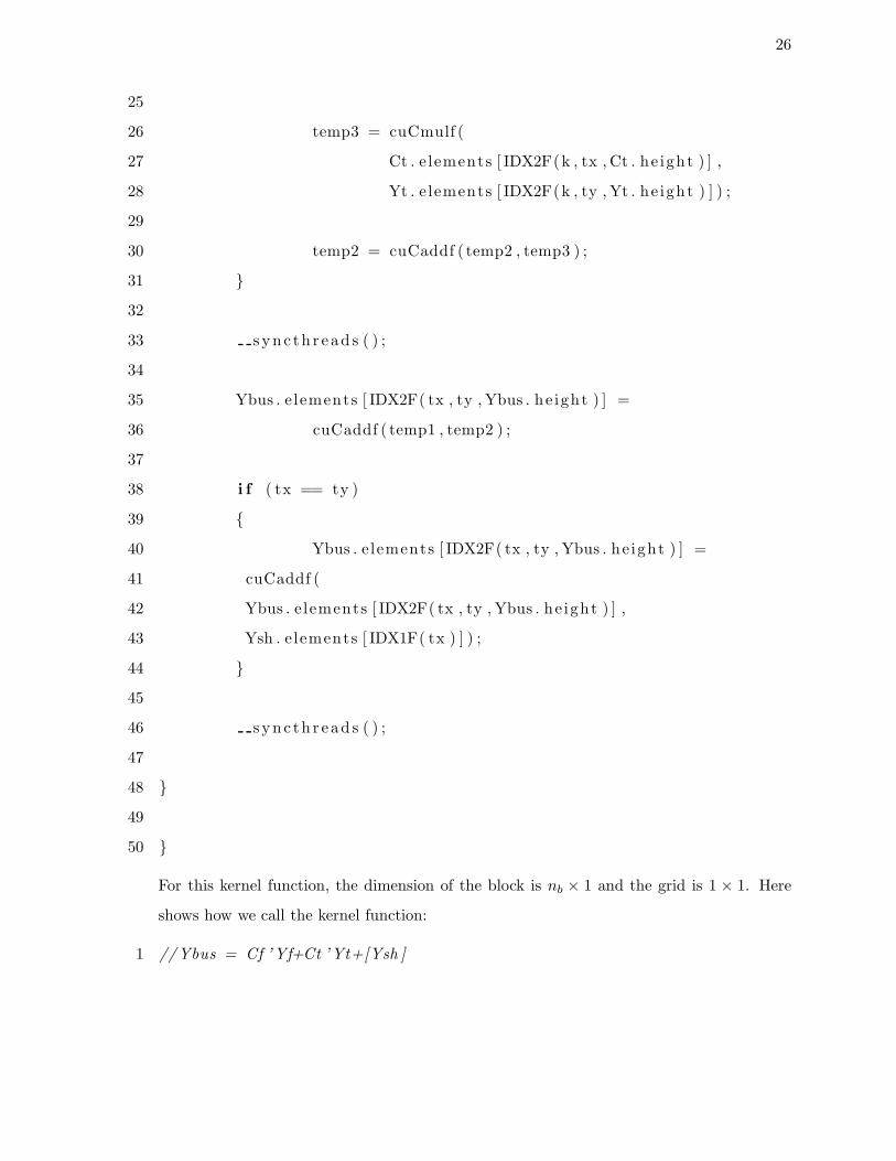
For this kernel function, the dimension of the block is nb × 1 and the grid is 1 × 1. Here

shows how we call the kernel function:

1 //Ybus = Cf ’Yf+Ct ’Yt+[Ysh ]

27

2 dim3 dimBlockYbus (YHost . Ybus . height , 1 , 1 ) ;

3 dim3 dimGridYbus ( 1 , 1 ) ;

4 MakeYbus<<<dimGridYbus , dimBlockYbus>>>

5 ( CfDevice , CtDevice , YDevice . Yf ,

6 YDevice . Yt , YshDevice , YDevice . Ybus ) ;

7

8 CheckCUDAKernalError ( ”Computer Ybus” ) ;

3.3 Solving Power Flow Problem

Here shows the steps for us to compute the solution for power flow problem:

1. Read data from data file

2. Convert the data into C structure

3. Create the bus admittance matrix Ybus

4. Initialize the complex voltage vector V(0) on host

5. Create the complex power injection vector S(0) on host

6. Transfer V(0), S(0) and Ybus from host to device

7. Run kernel functions to compute V

8. Compute S based on V

9. Transfer V and S from device to host

10. Free memory space on device

11. Print Results

In this section, we will mainly present how to use the kernel function to compute V.

Recall (2.36) and (2.37). Both have been written in an element-based format. Here, we

use the similar idea from the computation of Ybus, which uses each thread to compute

28

one element. Since this solution is founded by the Jacobi method, which is an iterative

algorithm, we use the algorithm described in Algorithm 1. Here is the listing shows the

algorithm in C:

1 for (unsigned int i = 0 ; i < 1000; i++)

2 {

3 // f o r PQ bus

4 VDeviceNew1 = VDevice ;

5 ComputePQBus<<<dimGridPQ , dimBlockPQ>>>

6 (YDevice . Ybus , BusTypeDevice . pq ,

7 SbusDevice , VDevice , VDeviceNew1 ) ;

8

9 // f o r PV bus

10 VDeviceNew2 = VDeviceNew1 ;

11 ComputePVBus<<<dimGridPV , dimBlockPV>>>

12 (YDevice . Ybus , BusTypeDevice . pv , SbusDevice ,

13 SbusDeviceNew , VDeviceNew1 , VDeviceNew2 , VmDevice ) ;

14

15 i f (maxElement (VDevice , VDevice2 ) < tau )

16 break ;

17

18 SbusDevice = SbusDeviceNew ;

19 VDevice = VDeviceNew2 ;

In this listing, the maximum number of iteration is 1000. In each iteration, we check the

maximum absolute error. If the error is smaller than tau, the Jacobi method converges.

In the listing above, we follow the computation algorithm for power flow system case

II, which is given in section 2.2.1. Firstly, we compute the complex voltage for PQ bus by

using (2.36). Here is a listing shows the kernel function:

1 g l o b a l void ComputePQBus( const cMatrix Ybus , const rVector pq ,

2 const cVector Sbus , const cVector Vold , cVector V)

29

3 {

4 unsigned int tx = threadIdx . x+1;

5 cuComplex temp1 , temp2 , temp3 ;

6 // tx = 2;

7 unsigned int k = pq . elements [ IDX1F( tx ) ] ;

8

9

10 temp2 = make cuFloatComplex ( 0 , 0 ) ;

11

12 temp1 = cuCdivf ( Sbus . e lements [ IDX1F(k ) ] ,

13 Vold . e lements [ IDX1F(k ) ] ) ;

14 temp1 = cuConjf ( temp1 ) ;

15

16

17

18 for (unsigned int j = 1 ; j <= Vold . l ength ; j++)

19 {

20 temp3 =

21 cuCmulf (

22 Ybus . e lements [ IDX2F(k , j , Ybus . he ight ) ] ,

23 Vold . e lements [ IDX1F( j ) ] ) ;

24

25 temp1 = cuCsubf ( temp1 , temp3 ) ;

26 }

27

28

29 temp1 = cuCdivf ( temp1 ,

30 Ybus . e lements [ IDX2F(k , k , Ybus . he ight ) ] ) ;

31

30

32 V. elements [ IDX1F(k ) ] =

33 cuCaddf (Vold . e lements [ IDX1F(k ) ] , temp1 ) ;

34 }

The dimension of the block is nb × 1 and the grid is 1× 1.

For the PV bus, we follow equation (2.37). This listing shows the kernel function:

1 g l o b a l void ComputePVBus( const cMatrix Ybus , const rVector pv ,

2 const cVector Sbusold , cVector Sbus , const cVector Vold ,

3 cVector V, const rVector f Vm)

4 {

5 unsigned int tx = threadIdx . x+1;

6 unsigned int k = pv . elements [ IDX1F( tx ) ] ;

7 cuComplex temp1 , temp2 ;

8

9 temp1 = make cuFloatComplex ( 0 , 0 ) ;

10

11 //Y(k , : ) ∗V

12 for (unsigned int j = 1 ; j<= Vold . l ength ; j++)

13 {

14 temp2 =

15 cuCmulf (Ybus . e lements [ IDX2F(k , j , Ybus . he ight ) ] ,

16 Vold . e lements [ IDX1F( j ) ] ) ;

17

18 temp1 = cuCaddf ( temp1 , temp2 ) ;

19 }

20

21

22 temp2 =

23 cuCmulf ( Vold . e lements [ IDX1F(k ) ] ,

24 cuConjf ( temp1 ) ) ;

31

25

26 Sbus . e lements [ IDX1F(k ) ] =

27 make cuFloatComplex (

28 cuCrea l f ( Sbusold . e lements [ IDX1F(k ) ] ) ,

29 cuCimagf ( temp2 ) ) ;

30

31 temp2 = cuCdivf ( Sbus . e lements [ IDX1F(k ) ] ,

32 Vold . e lements [ IDX1F(k ) ] ) ;

33 temp2 = cuConjf ( temp2 ) ;

34 temp2 = cuCsubf ( temp2 , temp1 ) ;

35 temp2 = cuCdivf ( temp2 ,

36 Ybus . e lements [ IDX2F(k , k , Ybus . he ight ) ] ) ;

37 temp2 = cuCaddf (Vold . e lements [ IDX1F(k ) ] , temp2 ) ;

38

39 V. elements [ IDX1F(k ) ] =

40 make cuFloatComplex (

41 cuCrea l f ( temp2 )/ cuCabsf ( temp2 )∗Vm. elements [ IDX1F(k ) ] ,

42 cuCimagf ( temp2 )/ cuCabsf ( temp2 )∗Vm. elements [ IDX1F(k ) ] ) ;

43

44

45 }

The dimension of the block is nb × 1 and the grid is 1× 1.

32

Chapter 4

Performance Analysis

In this project, we use the IEEE power flow test cases to evaluate the performance of the

CUDA-based power flow solver. We use the 9-bus case, 14-bus case, 57-bus case, 118-bus

case, and 300-bus case. In addition, the Matlab-based power flow software, MATPOWER

[12], is used as a benchmark.

Figure 4.1 shows the execution time for CUDA-based power flow solver and MAT-

POWER power flow solver. The MATPOWER ran on a PC with Intel(R) Pentium(R)

Dual CPU. The CPU has two threads and each thread operates at 2 GHz. The operation

system is 32-bit Windows 7. The Matlab version is 7.11.0.584 (R2010b). For the power flow

solver, the error tolerance τ is 10−4. The MATPOWER uses the Jacobi method as well.

Table 4 provides more details about Figure 4.1. Obviously, the CUDA-based power flow

solver is faster than the MATPOWER power flow solver, especially when the number of

bus is large. When the number of bus is small, such as 9-bus case and 14-bus case, the

execution time about 18 times and about 27 times faster than that of the MATPOWER.

Table 4.1: Execution time for power flow solver

number of bus CUDA MATPOWER ratio number(in second) (in second) (MATPOWER/CUDA) of iterations

9 0.040 0.7310 18.275 22014 0.020 0.550 27.500 11257 0.100 0.901 9.010 540118 0.188 5.030 26.755 1000300 0.378 14.752 39.027 1000

33

0 50 100 150 200 250 3000

5

10

15

number of bus

time

in s

econ

d

CUDAMATPOWER

Figure 4.1: Execution time for CUDA-based power flow solver and MATPOWER powerflow solver

34

When the number of bus increases to 57, the execution time ratio is only about 9. The

reason is the latency for reading data from global memory is increased. In CUDA GPU,

each thread reads the data from the global memory in a sequential way. When the latency

of computation on each thread is shorter than the latency of reading data from the memory,

the thread will just wait. When the number of buses increases to 118 and 300, the execution

time ratio also increases. Although the latency of reading data from global memory also

increases, at the same time, the latency of computation on each threads is extended as well.

At this point, the computation time is larger than the memory access time. Therefore, the

long latency of memory access is hired.

35

Chapter 5

Conclusion

In summary, in this project, we developed and converted the power flow solver from

its classic approach, which is implemented in sequential way, to a new approach, which is

implemented in a parallel algorithm. The developed parallel algorithm is implemented on

a CUDA-based GPU. Compared with the classic approach, the parallel approach can save

the execution time significantly.

There is still a large room for the further development on this algorithm. For example,

in the computation of Pi, Qi, |Vi| and θi, the elements of Ybus are remaining the same.

Currently, we save Ybus in the global memory. If we can save it in the constant memory,

the memory access latency can be reduced. In addition, if some elements can be transferred

from the global memory or the constant memory to the shared memory, the memory access

latency can be reduced as well.

36

Appendix A

NVIDIA GeForce GTS 250 GPU

Table A.1: NVIDIA GeForce GTS 250 GPU Specification

CUDA Driver Version: 3.20

CUDA Capability Major version number: 1.1

Total amount of global memory: 523829248 bytes

Multiprocessors: 16 MPs

Cores/MP: 8 Cores/MP

Cores: 128 Cores

Total amount of constant memory: 65536 bytes

Total amount of shared memory per block: 16384 bytes

Total number of registers available per block: 8192

Warp size: 32

Maximum number of threads per block: 512

Maximum sizes of each dimension of a block: 512 × 512 × 64

Maximum sizes of each dimension of a grid: 65535 × 65535 × 1

Maximum memory pitch: 2147483647 bytes

Clock rate: 1.50 GHz

Host to Device Bandwidth: 1081.5 MB/s

Device to Host Bandwidth: 924.7 MB/s

Device to Device Bandwidth: 48163.1 MB/s

37

Bibliography

[1] C. Nvidia, “NVIDIA CUDA C Programming Guide Version 3.2,” NVIDIA: Santa

Clara, CA, 2010.

[2] D. Kirk and W. Wen-mei, Programming massively parallel processors: A Hands-on

approach. Morgan Kaufmann Publishers Inc. San Francisco, CA, USA, 2010.

[3] R. Brown, “Impact of Smart Grid on distribution system design,” in Power and En-

ergy Society General Meeting-Conversion and Delivery of Electrical Energy in the 21st

Century, 2008 IEEE, pp. 1–4, Ieee, 2008.

[4] J. Grainger and W. Stevenson, Power system analysis, vol. 621. McGraw-Hill, 1994.

[5] S. Yamshchikov, A. Zhao, Financial Computations on the GPU. PhD thesis, WORCES-

TER POLYTECHNIC INSTITUTE, 2008.

[6] A. Bergen, Power systems analysis. Prentice Hall, Inc., Old Tappan, NJ, 1986.

[7] R. Zimmerman, C. Murillo-Sanchez, and R. Thomas, “MATPOWER: Steady-state

operations, planning, and analysis tools for power systems research and education,”

Power Systems, IEEE Transactions on, no. 99, pp. 1–8, 2011.

[8] R. Barrett, M. Berry, T. F. Chan, J. Demmel, J. Donato, J. Dongarra, V. Eijkhout,

R. Pozo, C. Romine, and H. V. der Vorst, Templates for the Solution of Linear Systems:

Building Blocks for Iterative Methods, 2nd Edition. Philadelphia, PA: SIAM, 1994.

[9] J. Nickolls, I. Buck, M. Garland, and K. Skadron, “Scalable parallel programming with

CUDA,” Queue, vol. 6, no. 2, pp. 40–53, 2008.

38

[10] Z. Zhang, Q. Miao, and Y. Wang, “CUDA-Based Jacobi’s Iterative Method,” in 2009

International Forum on Computer Science-Technology and Applications, pp. 259–262,

IEEE, 2009.

[11] C. Nvidia, “NVIDIA CUDA C Best Practices Guide Version 3.2,” NVIDIA: Santa

Clara, CA, 2010.

[12] R. Zimmerman, “Matpower 4.0 b4 Users Manual,” 2010.