Power Laws in Economicsand Finance

Xavier Gabaix

Stern School, New York University, New York, NY 10012; email:

xgabaix@stern.nyu.edu

Annu. Rev. Econ. 2009. 1:255–93

First published online as a Review in Advance on

June 4, 2009

The Annual Review of Economics is online at

econ.annualreviews.org

This article’s doi:

10.1146/annurev.economics.050708.142940

Copyright © 2009 by Annual Reviews.

All rights reserved

1941-1383/09/0904-0255$20.00

Key Words

scaling, fat tails, superstars, crashes

Abstract

A power law (PL) is the form taken by a large number of surprising

empirical regularities in economics and finance. This review

surveys well-documented empirical PLs regarding income and

wealth, the size of cities and firms, stock market returns, trading

volume, international trade, and executive pay. It reviews detail-

independent theoretical motivations that make sharp predictions

concerning the existence and coefficients of PLs, without requiring

delicate tuning of model parameters. These theoretical mechanisms

include random growth, optimization, and the economics of super-

stars, coupled with extreme value theory. Some empirical regula-

rities currently lack an appropriate explanation. This article

highlights these open areas for future research.

255

Ann

u. R

ev. E

con.

200

9.1.

Dow

nloa

ded

from

arj

ourn

als.

annu

alre

view

s.or

gby

NE

W Y

OR

K U

NIV

ER

SIT

Y -

BO

BST

LIB

RA

RY

on

08/1

1/09

. For

per

sona

l use

onl

y.

“Few if any economists seem to have realized the possibilities that such

invariants hold for the future of our science. In particular, nobody seems to

have realized that the hunt for, and the interpretation of, invariants of this

type might lay the foundations for an entirely novel type of theory.”

Schumpeter (1949, p. 155), discussing the Pareto law

1. INTRODUCTION

A power law (PL) is the form taken by a remarkable number of regularities, or laws, in

economics and finance. It is a relation of the type Y ¼ kXa, where Y and X are variables of

interest, a is the PL exponent, and k is typically an unremarkable constant.1 For example,

when X is multiplied by 2, then Y is multiplied by 2a(i.e., Y scales like X to the a). Despite

or perhaps because of their simplicity, scaling questions continue to be fecund in generat-

ing empirical regularities, and those regularities are sometimes among the most surprising

in the social sciences. They in turn motivate theories for their explanation, which often

require new ways to view economic issues.

Let us start, by example, with Zipf’s law, a particular case of a distributional PL. Pareto

(1896) found that the upper-tail distribution of the number of people with an income or

wealth S greater than a large x is proportional to 1=x z for some positive number z; i.e., itcan be written

PðS > xÞ ¼ k=xz ð1Þ

for some k. Importantly, the PL exponent z is independent of the units in which the law is

expressed. Zipf’s law2 states that z ’ 1. Understanding what gives rise to the relation and

explaining the precise value of the exponent (why it equals 1 rather than any other

number) are challenges that exist with PLs.

To visualize Zipf’s law, we can take a country (e.g., the United States) and order the

cities3 by population (e.g., New York as first, Los Angeles as second). Drawing a graph,

we place the log of the rank on the y axis (New York has log rank ln1, and Los Angeles has

a log rank ln 2), and on the x axis, we place the log of the population of the corresponding

city, which is called the size of the city. Figure 1 (following Krugman 1996 and Gabaix

1999a) shows the resulting plot for the 135 American metropolitan areas listed in the

Statistical Abstract of the United States for 1991.

The plot shows a straight line, which is rather surprising. There is no tautology causing

the data to automatically generate this shape. Indeed, running a linear regression yields

ln Rank ¼ 10:53� 1:005 ln Size; ð2Þ

1The fit of course may be approximate only in practice and may hold only over a bounded range.

2G.K. Zipf (1902–1950) was a Harvard linguist (for more information on him, see the 2002 special issue of

Glottometrics). Zipf’s law for cities was first noted by Auerbach (1913), whereas Estoup (1916) first discussed

Zipf’s law for words. Zipf explored the latter in different languages (a painstaking task of tabulation at the time,

with only human computing) and for different countries.

3The term city is, strictly speaking, a misnomer; agglomeration would be a better term. For our purpose, the city of

Boston includes Cambridge.

Zipf’s law: a power

law distribution with

exponent z ¼ 1, at

least approximately

Power law distribu-

tion: a distribution

that satisfies, at leastin the upper tail (and

perhaps up to an

upper cutoff signifying

border effects),PðSize > xÞ ’ kx�z,

where z is the power

law exponent, and k isa constant; also

known as a Pareto

distribution or scale-

free distribution

256 Gabaix

Ann

u. R

ev. E

con.

200

9.1.

Dow

nloa

ded

from

arj

ourn

als.

annu

alre

view

s.or

gby

NE

W Y

OR

K U

NIV

ER

SIT

Y -

BO

BST

LIB

RA

RY

on

08/1

1/09

. For

per

sona

l use

onl

y.

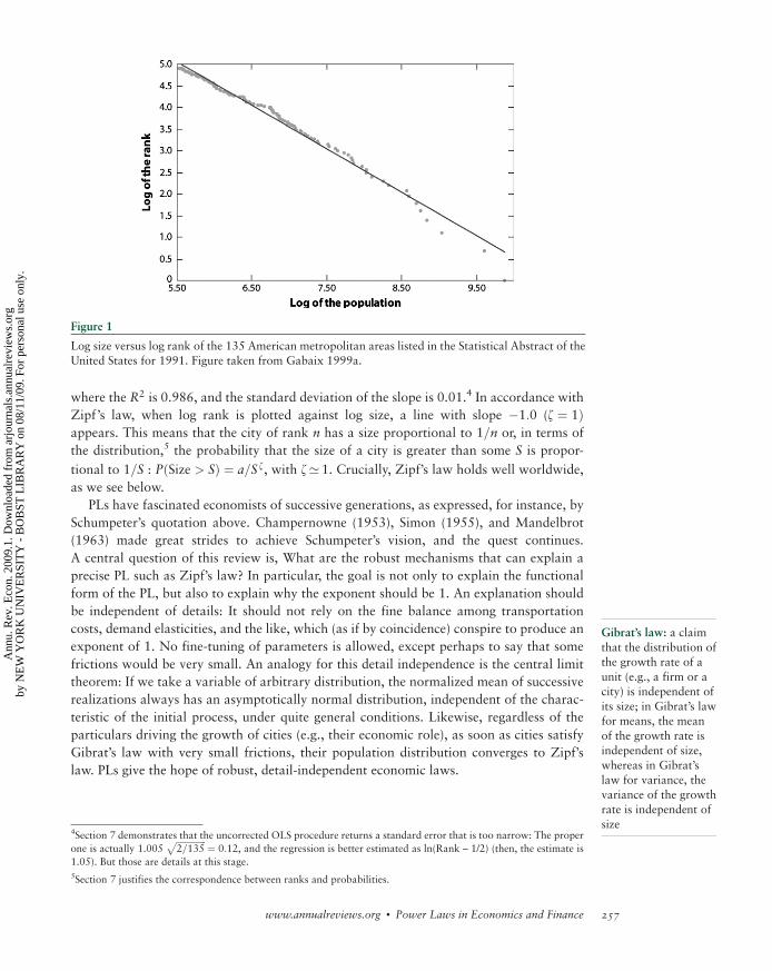
where the R2 is 0.986, and the standard deviation of the slope is 0.01.4 In accordance with

Zipf’s law, when log rank is plotted against log size, a line with slope �1:0 (z ¼ 1Þappears. This means that the city of rank n has a size proportional to 1=n or, in terms of

the distribution,5 the probability that the size of a city is greater than some S is propor-

tional to 1=S : PðSize > SÞ ¼ a=S z, with z’ 1. Crucially, Zipf’s law holds well worldwide,

as we see below.

PLs have fascinated economists of successive generations, as expressed, for instance, by

Schumpeter’s quotation above. Champernowne (1953), Simon (1955), and Mandelbrot

(1963) made great strides to achieve Schumpeter’s vision, and the quest continues.

A central question of this review is, What are the robust mechanisms that can explain a

precise PL such as Zipf’s law? In particular, the goal is not only to explain the functional

form of the PL, but also to explain why the exponent should be 1. An explanation should

be independent of details: It should not rely on the fine balance among transportation

costs, demand elasticities, and the like, which (as if by coincidence) conspire to produce an

exponent of 1. No fine-tuning of parameters is allowed, except perhaps to say that some

frictions would be very small. An analogy for this detail independence is the central limit

theorem: If we take a variable of arbitrary distribution, the normalized mean of successive

realizations always has an asymptotically normal distribution, independent of the charac-

teristic of the initial process, under quite general conditions. Likewise, regardless of the

particulars driving the growth of cities (e.g., their economic role), as soon as cities satisfy

Gibrat’s law with very small frictions, their population distribution converges to Zipf’s

law. PLs give the hope of robust, detail-independent economic laws.

Figure 1

Log size versus log rank of the 135 American metropolitan areas listed in the Statistical Abstract of theUnited States for 1991. Figure taken from Gabaix 1999a.

4Section 7 demonstrates that the uncorrected OLS procedure returns a standard error that is too narrow: The proper

one is actually 1.005ffiffiffiffiffiffiffiffiffiffiffiffiffiffi2=135

p ¼ 0:12, and the regression is better estimated as ln(Rank – 1/2) (then, the estimate is

1.05). But those are details at this stage.

5Section 7 justifies the correspondence between ranks and probabilities.

Gibrat’s law: a claim

that the distribution ofthe growth rate of a

unit (e.g., a firm or a

city) is independent of

its size; in Gibrat’s lawfor means, the mean

of the growth rate is

independent of size,

whereas in Gibrat’slaw for variance, the

variance of the growth

rate is independent of

size

www.annualreviews.org � Power Laws in Economics and Finance 257

Ann

u. R

ev. E

con.

200

9.1.

Dow

nloa

ded

from

arj

ourn

als.

annu

alre

view

s.or

gby

NE

W Y

OR

K U

NIV

ER

SIT

Y -

BO

BST

LIB

RA

RY

on

08/1

1/09

. For

per

sona

l use

onl

y.

Furthermore, one can gain insights into important questions by using PLs for a fresh

perspective. For instance, most people would agree that understanding the origins of stock

market crashes is an interesting question (e.g., for welfare, policy, and risk management).

Recent work (reviewed below) has indicated that stock market returns follow a PL;

moreover, it seems that stock market crashes are not outliers to a PL (Gabaix et al. 2005).

Hence, a unified economic mechanism might generate not only the crashes, but also a

whole PL distribution of crash-like events. Instead of having to theorize on just a few data

points (a rather unconstrained problem), one has to write a theory of the whole PL of large

stock market fluctuations. Therefore, thinking about the tail distribution may give us

insights both into the normal-time behavior of the market (inside the tails) and the most

extreme events. Understanding PLs may be key to understanding stock market crashes.

This article critically reviews the state of theory and empirics for PLs in economics and

finance.6 On the theory side, it emphasizes general methods that can be applied in varied

contexts. The theory sections are meant as a self-contained tutorial of the main methods to

deal with PLs.7 The empirical sections evaluate the many PLs found empirically, and their

connection to theory. The review concludes by highlighting some important open ques-

tions. Some readers may wish to skip directly to Sections 5 and 6, which contain a

summary of the PLs found empirically, along with the main theories proposed for their

explanation.

2. SIMPLE GENERALITIES

A countercumulative distribution PðS > xÞ ¼ kx�z corresponds to a density f ðxÞ ¼kzx�ðzþ1Þ. Some authors refer to 1þ z as the PL exponent (i.e., the PL exponent of the

density). However, theoretically, it is easier to work with the PL exponent of the counter-

cumulative distribution function because of transformation rule 8 listed below. Also, the

PL exponent z is independent of the measurement units (rule 7). This is why there is hope

for a universal statement (such as z ¼ 1). Finally, the lower the PL exponent is, the fatter

the tails are. If the income distribution has a lower PL exponent, then more inequality

exists between people in the top quantiles of income.

If a variable has a PL exponent z, all moments greater than z are infinite. This means

that, in bounded systems, the PL cannot fit exactly; there must be bounded size effects.

However, that is typically not a significant consideration. For instance, the distribution of

heights might be well approximated by a Gaussian, even though heights cannot be negative.

PLs also have excellent aggregation properties. The property of being distributed

according to a PL is conserved under addition, multiplication, polynomial transformation,

min, and max. The general rule is that, when combining two PL variables, the fattest (i.e.,

the one with the smallest exponent) PL dominates. For example, we can call zX the PL

exponent of variable X. The properties above also hold if zX ¼ þ1 (i.e., X is thinner than

any PL for instance, if X is a Gaussian).

6This survey has limitations and is by no means exhaustive. Also, it cannot do justice to the interesting movement of

econophysics, which comprises a large group of physicists and some economists that use statistical physics to find

regularities in economic data and write new models. This field is a good source of results on PLs, and its mastery

exceeds the author’s expertise. The models are also not yet easily readable by economists. Durlauf (2005) provides a

partial survey.

7The theory sections draw from Gabaix (1999a), Gabaix & Ioannides (2004), Gabaix & Landier (2008), and my

New Palgrave entry on the same topic.

258 Gabaix

Ann

u. R

ev. E

con.

200

9.1.

Dow

nloa

ded

from

arj

ourn

als.

annu

alre

view

s.or

gby

NE

W Y

OR

K U

NIV

ER

SIT

Y -

BO

BST

LIB

RA

RY

on

08/1

1/09

. For

per

sona

l use

onl

y.

Indeed, for X1; :::;Xn independent random variables and a positive constant a, we have

the following formulas (see Jessen & Mikosch 2006 for a survey)8, implying that PLs

beget new PLs (the inheritance mechanism for PLs):

zX1þ���þXn¼ minðzX1

; . . . ; zXnÞ; ð3Þ

zX1�����Xn¼ minðzX1

; . . . ; zXnÞ; ð4Þ

zmaxðX1;...;XnÞ ¼ minðzX1; . . . ; zXn

Þ; ð5Þ

zminðX1 ;...;XnÞ ¼ zX1þ � � � þ zXn

; ð6Þ

zaX ¼ zX; ð7Þ

zXa ¼ zXa: ð8Þ

For instance, if X is a PL variable for zX51 and Y is a PL variable with an exponent

zY � zX, then Xþ Y;X� Y, and maxðX;YÞ are still PLs with the same exponent zX:Thisproperty holds when Y is normal, lognormal, or exponential, in which case zY ¼ 1:

Hence, multiplying by normal variables, adding nonfat tail noise, or summing over inde-

pendent and identically distributed (i.i.d.) variables preserves the exponent.

These properties make theorizing with PLs streamlined. Also, they give the empiricist

hope that those PLs can be measured, even if the data are noisy. Although noise affects

statistics (e.g., variances), it will not affect the PL exponent. PL exponents carry over the

essence of the phenomenon: Smaller order effects do not affect them. Also, the above

formulas indicate how to use PL variables to generate new PLs.

3. THEORY I: RANDOM GROWTH

This section provides a key mechanism that explains economic PLs: proportional random

growth. Other mechanisms are explored in Section 4. Moreover, Bouchaud (2001),

Mitzenmacher (2003), Sornette (2004), and Newman (2005) survey mechanisms from a

physics perspective.

3.1. Proportional Random Growth Leads to a Power Law

A central mechanism for explaining distributional PLs is proportional random growth. The

process originates with Yule (1925), and it was developed in economics by Champernowne

(1953) and Simon (1955) and rigorously studied by Kesten (1973). To illustrate the general

mechanism (and guide intuition), we take the example of an economy with a continuum of

cities, with mass. Below we clearly show that the model applies more generally. We let Pit be

the population of city i and P�t the average population size. We define Sit ¼ Pit=P�t as the

8Several proofs are quite easy. For example, using Equation 8, if PðX > xÞ ¼ kx�z, then PðXa > xÞ ¼PðX > x1=aÞ ¼ kx�z=a, so zXa ¼ zX=a.

www.annualreviews.org � Power Laws in Economics and Finance 259

Ann

u. R

ev. E

con.

200

9.1.

Dow

nloa

ded

from

arj

ourn

als.

annu

alre

view

s.or

gby

NE

W Y

OR

K U

NIV

ER

SIT

Y -

BO

BST

LIB

RA

RY

on

08/1

1/09

. For

per

sona

l use

onl

y.

normalized population size. Throughout this review, we reason in normalized sizes,9 so that

the average city size remains constant (here at a value 1). Such a normalization is impor-

tant in any economic application. As we want to discuss the steady-state distribution of

cities (or, for example, incomes), we need to normalize to ensure such a distribution exists.

Let us suppose that each city i has a population Sit, which increases by a gross growth

rate g itþ1 from time t to time t þ 1:

Sitþ1 ¼ gitþ1Sit: ð9Þ

We assume that the growth rates gitþ1 are i.i.d., with density f ðgÞ, at least in the upper

tail. We let GtðxÞ ¼ PðSit > xÞ, which is the countercumulative distribution function of the

city size. The equation of motion of Gt is

Gtþ1ðxÞ ¼ PðSitþ1 > xÞ ¼ P gitþ1Sit > x

� � ¼ P Sit >x

gitþ1

0@

1A

¼ R10 Gt

�x

g

�f ðgÞdg:

Hence, its steady-state distribution G, if it exists, satisfies

G Sð Þ ¼Z 1

0

GS

g

� �f ðgÞdg: ð10Þ

One can try the functional form GðSÞ ¼ k=Sz; where k is a constant, which gives

1 ¼ R10 gzf ðgÞdg; i.e.

E½gz� ¼ 1: ð11ÞHence, if the steady-state distribution is Pareto in the upper tail, then the exponent z is thepositive root of Equation 11 (if such a root exists).10

Equation 11 is fundamental to random growth processes. To the best of my knowledge,

it was first derived by Champernowne in his 1937 doctoral dissertation and then pub-

lished in 1953 (Champernowne 1953). (Even then, publication delays in economics could

be quite long.) The main predecessor to Champernowne, Yule (1925), does not contain it.

Hence, I propose the term “Champernowne’s equation” for Equation 11.11 Champer-

nowne’s equation expresses the following. Let us consider a random growth process that,

to the leading order, can be written Stþ1 � gtþ1St for large size, where g is an i.i.d. random

variable. Then, if there is a steady-state distribution, it is a PL with exponent z, where z isthe positive solution of Equation 11 and can be related to the distribution of the (normal-

ized) growth rate g.Above we assume that the steady-state distribution exists. To guarantee its existence,

some deviations from a pure random growth process (i.e., some friction) need to be added.

Indeed, if we did not have friction, we would not get a PL distribution. If Equation 9 held

9Economist Levy and physicist Solomon (1996) instigated a resurging interest in Champernowne’s random growth

process with lower bound and, to the best of my knowledge, presented the first normalization by the average. Wold

& Wittle (1957) may have been the first to introduce normalization by a growth factor in a random growth model.

10Later we see arguments showing that the steady-state distribution is indeed necessarily a PL.

11Champernowne (similar to Simon) also programmed chess-playing computers (with Alan Turing) and invented

Champernowne’s number, which consists of a decimal fraction in which the decimal integers are written sucessively:

0.01234567891011121314. . .99100101. . . . It is a challenge in computer science as it appears random to most tests.

260 Gabaix

Ann

u. R

ev. E

con.

200

9.1.

Dow

nloa

ded

from

arj

ourn

als.

annu

alre

view

s.or

gby

NE

W Y

OR

K U

NIV

ER

SIT

Y -

BO

BST

LIB

RA

RY

on

08/1

1/09

. For

per

sona

l use

onl

y.

throughout the distribution, then we would have ln Sit ¼ ln Si0 þPt

s¼1ln gitþ1, and the dis-

tribution would be lognormal without a steady state [as varðln SitÞ ¼ varðln Si0Þ þ varðln gÞt,the variance growth without bound]. This is Gibrat’s (1931) observation. Hence, to ensure

that the steady-state distribution exists, one needs some friction to prevent cities or firms

from becoming too small.

Potential frictions include a positive constant added in Equation 9 that prevents small

entities from becoming too small (which are described in detail in Section 3.3) and a lower

bound for sizes enforced by a reflecting barrier (see Section 3.4). Economically, those

forces might be a positive probability of death, a fixed cost that prevents very small firms

from operating profitably or cheap rents for small cities, which induces them to grow

faster (see below). Importantly, the particular force that affects small sizes typically does

not affect the PL exponent in the upper tail. In Equation 11, only the growth rate in the

upper tail matters. The above random growth process also can explain the Pareto distribu-

tion of wealth, interpreting Sit as the wealth of individual i.

3.2. Zipf’s Law: A First Pass

We see that proportional random growth leads to a PL with some exponent z. Why should

the exponent 1 appear in so many economic systems (e.g., cities, firms, exports)? Here we

begin to answer that question (which is developed further below).12 Let us call the mean

size of units S�, which is a constant because we have normalized sizes by the average size

of units. Let us suppose that the random growth process (Equation 9) holds throughout

most of the distribution, rather than just in the upper tail. We take the expectation on

Equation 9, which gives S�¼ E½Stþ1� ¼ E½g�E½St� ¼ E½g� S�. Hence,

E½g� ¼ 1:

(In other words, as the system has a constant size, we need E½Stþ1� ¼ E½St�: The expected

growth rate is 0 so E½g� ¼ 1.) This implies Zipf’s law as z ¼ 1 is the positive solution of

Equation 11. Hence, the steady-state distribution is Zipf, with an exponent z ¼ 1.

The above derivation is not quite rigorous because we need to introduce some friction

for the random process (Equation 9) to have a solution with a finite mean size. In other

terms, to get Zipf’s law, we need a random growth process with small frictions. The

following sections introduce frictions and make the above reasoning rigorous, delivering

exponents very close to 1.

When frictions are large (e.g., with a reflecting barrier or the Kesten process in Gabaix

1999a, appendix 1), a PL arises but Zipf’s law does not hold exactly. In those cases, small

units grow faster than large units. Then, the normalized mean growth rate of large cities is

less than 0; i.e., E½g�51, which implies z > 1. In sum, proportional random growth with

frictions leads to a PL and proportional random growth with small frictions leads to a

special type of PL, Zipf’s law.

3.3. Rigorous Approach via Kesten Processes

One case in which random growth processes have been completely rigorously treated

involves the Kesten processes. Let us consider the process St ¼ AtSt�1 þ Bt, where ðAt;BtÞ12Here I follow Gabaix (1999a). See the later sections for more analytics on Zipf’s law, along with some history.

www.annualreviews.org � Power Laws in Economics and Finance 261

Ann

u. R

ev. E

con.

200

9.1.

Dow

nloa

ded

from

arj

ourn

als.

annu

alre

view

s.or

gby

NE

W Y

OR

K U

NIV

ER

SIT

Y -

BO

BST

LIB

RA

RY

on

08/1

1/09

. For

per

sona

l use

onl

y.

are i.i.d. random variables. If St has a steady-state distribution, then the distribution of

St and ASt þ B is the same, something we can write S¼dASþ B . The basic formal result is

from Kesten (1973) and was extended by Vervaat (1979) and Goldie (1991).

Theorem 1: (Kesten 1973) For some z > 0,

E½jAjz� ¼ 1; ð12Þ

and E jAjz max�lnðAÞ; 0

�h i51, 05E½jBjz�51. Let us also suppose that B=ð1� AÞ is

not degenerate (i.e., it can take more than one value), and the conditional distribution

of ln jAj given A 6¼ 0 is nonlattice (i.e., it has a support that is not included in lZ for

some l). Then there are constant kþ and k�, at least one of them being positive, such that

xzPðS > xÞ ! kþ; xzPðS5� xÞ ! k�; ð13Þas x ! 1, where S is the solution of S¼dASþ B. Furthermore, the solution of the recur-

rence equation Stþ1 ¼ Atþ1St þ Btþ1 converges in probability to S as t ! 1.

The first condition is none other than Champernowne’s equation (Equation 11) when

the gross growth rate is always positive. The condition E½jBjz�51 means that B does not

have fatter tails than a PL with exponent z (otherwise, the PL exponent of S would

presumably be that of B).

Kesten’s theorem formalizes the heuristic reasoning of Section 3.2. However, that same

heuristic logic makes it clear that a more general process still has the same asymptotic

distribution. For instance, one may conjecture that the process St ¼ AtSt�1 þ fðSt�1;BtÞ,with fðS;BtÞ ¼ oðSÞ for large x, should have an asymptotic PL tail in the sense of Equa-

tion 13, with the same exponent z. Such a result does not seem to have been proven yet.

To illustrate the power of the Kesten framework, let us examine an application to the

ARCH (autoregressive conditional heteroskedastic) processes: s2t ¼ as2t�1e2t þ b, and the

return is etst�1, with et independent of st�1. Then, we are in the framework of Kesten’s

theory, with St ¼ s2t , At ¼ ae2t , and Bt ¼ b. Hence, squared volatility s2t follows a PL distri-

bution with exponent z such that E½ðae2tþ1Þz� ¼ 1. By rule 8, this means that zs ¼ 2z. AsE½e2ztþ1�5 1, ze � 2z, and rule 4 implies that returns follow a PL, zr ¼ minðzs; zeÞ ¼ 2z. Thesame reasoning demonstrates that GARCH (generalized ARCH) processes have PL tails.

3.4. Continuous-Time Approach

This subsection, although more technical, uses continuous time to make calculations easier.

3.4.1. Basic tools, and random growth with reflecting barriers. Let us consider the con-

tinuous time process

dXt ¼ mðXt; tÞdt þ sðXt; tÞdzt;where zt is a Brownian motion, and Xt can be thought of as the size of an economic unit

(e.g., a city or a firm, perhaps in normalized units). The process Xt could be reflected at

some points. Let us call f ðx; tÞ the distribution at time t. To describe the evolution of the

distribution, given the initial conditions f ðx; t ¼ 0Þ, we use the forward Kolmogorov

equation as our basic tool:

@tf ðx; tÞ ¼ �@x½mðx; tÞf ðx; tÞ� þ @xxs2ðx; tÞ

2f ðx; tÞ

; ð14Þ

262 Gabaix

Ann

u. R

ev. E

con.

200

9.1.

Dow

nloa

ded

from

arj

ourn

als.

annu

alre

view

s.or

gby

NE

W Y

OR

K U

NIV

ER

SIT

Y -

BO

BST

LIB

RA

RY

on

08/1

1/09

. For

per

sona

l use

onl

y.

where @tf ¼ @f=@t, @xf ¼ @f=@x, and @xxf ¼ @2f=@x2. Its major application is to calculate

the steady-state distribution f ðxÞ, in which case @tf ðxÞ ¼ 0.

As a central application, let us solve for the steady state of a random growth process.

We have mðXÞ ¼ gX and sðXÞ ¼ vX. In terms of the discrete time model (Equation 9), this

corresponds, symbolically, to gt ¼ 1þ gdt þ vdzt. We assume that the process is reflected

at a size Smin: If the process goes below Smin, it is brought back at Smin. Above Smin, it

satisfies dSt ¼ mðStÞdt þ sðStÞdzt. Symbolically, Stþdt ¼ max½Smin; St þ mðStÞdt þ sðStÞdzt�.Thus g and v are the mean and standard deviation of the growth rate of firms, respectively,

when they are above the reflecting barrier.

We can solve the steady state by inserting f ðx; tÞ ¼ f ðxÞ into Equation 14, so that

@tf ðx; tÞ ¼ 0. For x > Smin, the forward Kolmogorov equation gives

0 ¼ �@x½gxf ðxÞ� þ @xxv2

2x2f ðxÞ

:

If we insert a candidate PL solution,

f ðxÞ ¼ Cx�z�1; ð15Þ

into the forward Kolmogorov Equation, we get

0 ¼ �@x½gxCx�z�1� þ @xxv2x2

2Cx�z�1

¼ Cx�z�1 gzþ v2

2ðz� 1Þz

;

which has two possible solutions. One solution, z ¼ 0, does not correspond to a finite

distribution:R1Smin

f ðxÞdx diverges. Thus, the correct solution is

z ¼ 1� 2g

v2; ð16Þ

which gives the PL exponent of the distribution.13 For the mean of the process to be finite,

we need z > 1; hence g50. As the total growth rate of the normalized population is 0, and

the growth rate of reflected units is necessarily positive, the growth rate of nonreflected

units (g) must be negative.

Using economic arguments that the distribution has to go smoothly to 0 for large x, one

can show that Equation 15 is the only solution. Ensuring that the distribution integrates to

a mass 1 gives the constant C and the distribution f ðxÞ ¼ zx�z�1Szmin; i.e.,

PðS > xÞ ¼ x

Smin

� ��z

: ð17Þ

Hence, random growth with a reflecting lower barrier generates a Pareto—an insight from

Champernowne (1953).

Why then would Zipf’s law hold? The mean size is

S�¼Z 1

Smin

xf ðxÞdx ¼Z 1

Smin

x�zx�z�1Szmindx ¼ zSzmin

x�zþ1

�zþ 1

1Smin

¼ zz� 1

Smin:

13This also comes heuristically from Equation 11, applied to gt ¼ 1þ gdt þ sdzt, and by Ito’s lemma

1 ¼ E½gzt � ¼ 1þ zgdt þ zðz� 1Þv2=2dt.

www.annualreviews.org � Power Laws in Economics and Finance 263

Ann

u. R

ev. E

con.

200

9.1.

Dow

nloa

ded

from

arj

ourn

als.

annu

alre

view

s.or

gby

NE

W Y

OR

K U

NIV

ER

SIT

Y -

BO

BST

LIB

RA

RY

on

08/1

1/09

. For

per

sona

l use

onl

y.

Thus, we see that the PL exponent is14

z ¼ 1

1� Smin= S�: ð18Þ

We find again reasoning for Zipf’s law: When the zone of frictions is very small (Smin= S�

small), the PL exponent goes to 1. But, of course, it can never exactly reach Zipf’s law: In

Equation 18, the exponent is always above 1. Another way to stabilize the process, so that

it has a steady-state distribution, is to have a small death rate, which is discussed below.

3.4.2. Extensions with birth, death, and jumps. We can enrich the process with death and

birth. We assume that one unit of size x dies with Poisson probability dðx; tÞ per unit oftime dt. We also assume that a quantity jðx; tÞ of new units is born at size x. Let us call

nðx; tÞdx the number of units with size ðx; xþ dxÞ. The forward Kolmogorov equation

describes its evolution as

@tnðx; tÞ ¼ �@x½mðx; tÞnðx; tÞ� þ @xxs2ðx; tÞ

2nðx; tÞ

� dðx; tÞnðx; tÞ þ jðx; tÞ: ð19Þ

As an application, we consider a random growth law model in which existing units grow

at rate g and have volatility v. Units die with a Poisson rate d and are immediately reborn

at a size S. Therefore, for simplicity, we assume a constant size for the system: The

number of units is constant. There is no reflecting barrier; instead, the death and rebirth

processes stabilize the steady-state distribution (see also Malevergne et al. 2008).

The forward Kolmogorov equation (outside the point of re-injection S), evaluated at

the steady-state distribution f ðxÞ, is

0 ¼ �@x½gxf ðxÞ� þ @xxv2x2

2f ðxÞ

� df ðxÞ:

We look for elementary solutions of the form f ðxÞ ¼ Cx�z�1. Inserting this into the above

equation gives

0 ¼ �@x½gxx�z�1� þ @xxv2x2

2x�z�1

� dx�z�1;

in other words,

0 ¼ zgþ v2

2zðz� 1Þ � d: ð20Þ

This equation now has a negative root z� and a positive root zþ. The general solution

for x, different from S, is f ðxÞ ¼ C�x�z��1 þ Cþx�zþ�1. Because units are re-injected

at size S, the density f could be positive singular at that value. The steady-state

distribution is15

14In a simple model of cities, the total population is exogenous, and the number of cities is exogenous; hence the

total average (normalized) size per city S� is exogenous. Likewise, volatility v and Smin are exogenous. However, the

mean growth rate g of the cities that are not reflected is endogenous. It will self-organize, so as to satisfy Equations

16 and 18. Still, the total growth rate of normalized size remains 0.

15For x > S, the solution must be integrable when x ! 1: that imposes C� ¼ 0. For x5S, the solution must be

integrable when x ! 0: that imposes Cþ ¼ 0.

264 Gabaix

Ann

u. R

ev. E

con.

200

9.1.

Dow

nloa

ded

from

arj

ourn

als.

annu

alre

view

s.or

gby

NE

W Y

OR

K U

NIV

ER

SIT

Y -

BO

BST

LIB

RA

RY

on

08/1

1/09

. For

per

sona

l use

onl

y.

f ðxÞ ¼ Cðx=SÞ�z��1 for x5 SCðx=SÞ�zþ�1 for x > S

;

�

and the constant C ¼ �zþz�=½ðzþ � z�ÞS�. This is the double Pareto (Champernowne

1953, Reed 2001).

We can study how Zipf’s law arises from such a system. The mean size of the system is

S�¼ S�zþz�

ðzþ � 1Þð1� z�Þ: ð21Þ

As Equation 20 implies that zþz� ¼ �2d=v2, Equation 21 can be rearranged as

ðzþ � 1Þ 1þ 2d=v2

zþ

� �¼ S

S�2d=v2:

Hence, we obtain Zipf’s law (zþ ! 1) if either (a) SS�! 0 (re-injection is done at very small

sizes) or (b) d ! 0 (the death rate is very small). We see again that Zipf’s law arises when

there is random growth in most of the distribution and frictions are very small.

As another enhancement, we can consider jumps. With some probability pdt, a jump

occurs, and the process size is multiplied by G�t , which is stochastic and i.i.d.:

Xtþdt ¼ ð1þ gdt þ vdzt þG�tdJtÞXt, where dJt is a jump process (dJt ¼ 0 with probability

1� pdt and dJt ¼ 1 with probability pdt). This corresponds to a death rate dðx; tÞ ¼ p and

an injection rate jðx; tÞ ¼ pE½nðx=G; tÞ=G�. The latter results from the injection at a size

above x coming from a size above x=G. Hence, using Equation 19, the forward Kolmo-

gorov equation is

@tnðx; tÞ ¼ �@x½mðx; tÞnðx; tÞ� þ @xxs2ðx; tÞ

2nðx; tÞ

þ pE

nðx=G; tÞG

� nðx; tÞ

; ð22Þ

where the last expectation is over the realizations of G.

Combining Equations 19 and 22, the forward Kolmogorov equation becomes

@tnðx; tÞ ¼ �dðx; tÞnðx; tÞ þ jðx; tÞ � @x½mðx; tÞnðx; tÞ� þ @xxs2ðx; tÞ

2nðx; tÞ

24

35

þpEnðx=G; tÞ

G� nðx; tÞ

24

35;

ð23Þ

featuring the impact of death (d), birth (j), mean growth (m), volatility (s), and jumps (G).

For instance, we can take random growth with mðxÞ ¼ gx, sðxÞ ¼ vx, and death rate d,and apply this to a steady-state distribution nðx; tÞ ¼ f ðxÞ. Inserting f ðxÞ ¼ f ð0Þx�z�1 into

Equation 23 gives

0 ¼ �dx�z�1 � @xðgx�zÞ þ @xxvx2

2x�z�1

� �þ E

x

G

� ��z�1 1

G� 1

;

in other words,

0 ¼ �dþ gzþ v2

2zðz� 1Þ þ pE½Gz � 1�: ð24Þ

We see that the PL exponent z is lower (the distribution has fatter tails) when the

death rate is lower, the growth rate, and the variance are higher (in the domain z > 1).

www.annualreviews.org � Power Laws in Economics and Finance 265

Ann

u. R

ev. E

con.

200

9.1.

Dow

nloa

ded

from

arj

ourn

als.

annu

alre

view

s.or

gby

NE

W Y

OR

K U

NIV

ER

SIT

Y -

BO

BST

LIB

RA

RY

on

08/1

1/09

. For

per

sona

l use

onl

y.

All those forces make it easier to obtain large units (e.g., cities or firms) in the steady-state

distribution.16

3.4.3. Deviations from a power law. As the possibility exists that Gibrat’s law might not

hold exactly, it is worth examining the case in which cities grow randomly with expected

growth rates and standard deviations that depend on their sizes (Gabaix 1999a). That is,

the (normalized) size of city i at time t varies according to

dStSt

¼ g Stð Þdt þ v Stð Þdzt; ð25Þ

where gðSÞ and v2ðSÞ denote the instantaneous mean and variance of the growth rate

of a size S city, respectively, and zt is a standard Brownian motion. In this case, the

limit distribution of city sizes converges to a law with a local Zipf exponent, z Sð Þ ¼� S

f ðSÞdf ðSÞdS � 1; where f ðSÞ denotes the stationary distribution of S: Working with the for-

ward Kolmogorov equation associated with Equation 25, we yield

@

@tf S; tð Þ ¼ � @

@S

�gðSÞSf ðS; tÞ

�þ 1

2

@2

@S2

�v2ðSÞS2f ðS; tÞ

�: ð26Þ

The local Zipf exponent associated with the limit distribution, when @@t f S; tð Þ ¼ 0, is

given by

z Sð Þ ¼ 1� 2gðSÞv2ðSÞ þ

S

v2ðSÞ@v2ðSÞ@S

; ð27Þ

where gðSÞ is relative to the overall mean for all city sizes. As verification of Zipf’s law,

when the growth rate of normalized sizes (as all cities grow at the same rate) is

0 [gðSÞ ¼ 0], and variance is independent of firm size [@v2ðSÞ@S ¼ 0], then the exponent is

zðSÞ ¼ 1. Conversely, if small cities or firms have larger standard deviations than large

cities (perhaps because their economic base is less diversified), then @v2ðSÞ@S 50, and the

exponent (for small cities) would be lower than 1.

Equation 27 allows us to study deviations from Gibrat’s law. For instance, it is conceiv-

able that smaller cities have a higher variance than large cities. Variance would decrease

with size for small cities and then asymptote to a variance floor for large cities. This could

result from large cities still having an undiversified industry base, such as New York and

Los Angeles. Using Equation 27 in the baseline case in which all cities have the same

growth rate [which forces gðSÞ ¼ 0 for the normalized sizes], we get zðSÞ ¼ 1þ@ ln v2ðSÞ=ln S, with @ ln v2ðSÞ=@ ln S50 in the domain in which volatility decreases with

size. Therefore, this may explain why the z coefficient might be lower for smaller cities.

3.5. Additional Remarks on Random Growth

We conclude with a few additional remarks on random growth models.

3.5.1. Simon’s model and others. The simplest random growth model is Steindl’s (1965).

In this model, new cities are born at a rate n, with a constant initial size, and existing cities

grow at a rate g. Therefore, the distribution of new cities is in the form of a PL, with

16The Zipf benchmark with z ¼ 1 has a natural interpretation, which will be discussed in a future paper.

266 Gabaix

Ann

u. R

ev. E

con.

200

9.1.

Dow

nloa

ded

from

arj

ourn

als.

annu

alre

view

s.or

gby

NE

W Y

OR

K U

NIV

ER

SIT

Y -

BO

BST

LIB

RA

RY

on

08/1

1/09

. For

per

sona

l use

onl

y.

an exponent z ¼ n=g, as a quick derivation shows.17 However, this is quite problematic

as an explanation for Zipf’s law. It does deliver the desired result (namely, the exponent

of 1), but only by assuming that historically n ¼ g, which is quite implausible empirically,

especially for mature urban systems, for which it is likely that n5g. Yet Steindl’s model

gives us a simple way to understand Simon’s (1955) model (for a particularly clear exposi-

tion of Simon’s model, see Krugman 1996, and Yule 1925 for an antecedent). New

migrants (e.g., of mass 1) arrive each period. With probability p, they form a new city,

whereas with probability 1� p, they go to an existing city. When moving to an existing

city, the probability that they choose a given city is proportional to its population.

This model generates a PL, with exponent z ¼ 1=ð1� pÞ. Thus, the exponent of 1 has a

natural explanation: The probability p of new cities is small. This seems quite successful,

and, indeed, this makes Simon’s model an important, first explanation of Zipf’s law via

small frictions. However, Simon’s model suffers from two drawbacks that limit its ability

to explain Zipf’s law.18 First, it suffers from the same problem as Steindl’s model (Gabaix

1999a, appendix 3). If the total population growth rate is g0, it generates a growth rate in

the number of cities equal to n ¼ g0 and a growth rate of existing cities equal to

g ¼ ð1� pÞg0. Hence, Simon’s model implies that the rate of growth of the number of

cities has to be greater than the rate of growth of the population of the existing cities. This

essential feature is probably empirically unrealistic (especially for mature urban systems

such as those of Western Europe).19 Second, the model predicts that the variance of the

growth rate of an existing unit of size S should be v2ðSÞ ¼ k=S. (Indeed, in this model a

unit of size S receives, metaphorically speaking, a number of independent arrival shocks

proportional to S.) Larger units have a much smaller standard deviation of growth rate

than small cities. Such a strong departure from Gibrat’s law for variance is almost certain-

ly not true for cities (Ioannides & Overman 2003) or firms (Stanley et al. 1996). This

violation of Gibrat’s law for variances seems to have been overlooked by researchers.

Simon’s model has enjoyed a great renewal in the literature on the evolution of Web sites

(Barabasi & Albert 1999). Hence, it seems useful to test Gibrat’s law for variance in the

context of Web site evolution and accordingly correct the model.

Until the late 1990s, the central argument for an exponent of 1 for the Pareto was still

based on Simon’s (1955) model. Other models (e.g., surveyed in Carroll 1982 and Krugman

1996) had no clear economic meaning (e.g., entropy maximization) or did not explain why

the exponent should be 1. Then, two independent literatures, in physics and economics,

entered the fray. In an influential contribution, Levy & Solomon (1996) extended the Cham-

pernowne (1953) model to one with coupling between units. Although they do not explicitly

discuss the Zipf case, it is possible to derive a Zipf-like result using their framework. Later,

Malcai et al. (1999) (see below) described a mechanism for Zipf’s law, emphasizing finite-size

effects. Marsili & Zhang’s (1998) model can be tuned to yield Zipf’s law, but that tuning

implies that gross flow in and out of a city is proportional to the city size to the power 2

(rather than to the power 1), which is most likely counterfactual and too large for large

17The cities of size greater than S are the cities of age greater than a ¼ lnS=g. Because of the form of the birth

process, the number of these cities is proportional to e�na ¼ e�nln S=g ¼ S�n=g, which gives the exponent z ¼ n=g.18Krugman (1996) also describes a third drawback: Simon’s model may converge too slowly compared to historical

timescales.

19This can be fixed by assuming that the birth size of a city grows at a positive rate. But then the model is quite

different, and the next problem remains.

www.annualreviews.org � Power Laws in Economics and Finance 267

Ann

u. R

ev. E

con.

200

9.1.

Dow

nloa

ded

from

arj

ourn

als.

annu

alre

view

s.or

gby

NE

W Y

OR

K U

NIV

ER

SIT

Y -

BO

BST

LIB

RA

RY

on

08/1

1/09

. For

per

sona

l use

onl

y.

cities. Zanette & Manrubia (1997; Manrubia & Zanette 1998) and Marsili et al. (1998b)

presented models that can generate Zipf’s law [see also a critique by Marsili et al. (1998a),

followed by Zanette & Manrubia’s reply]. Zanette & Manrubia postulated a growth

process that can take only two values and emphasized an analogy with the physics of

intermittent, turbulent behavior. Marsili et al. (1998b) analyzed a rich portfolio choice

problem, studying the limit of weak coupling between stocks and highlighting the analogy

with polymer physics. As a result, their interesting works arguably may not elucidate the

generality of the mechanism for Zipf’s law outlined in Section 3.2.

In the field of economics, Krugman (1996) revived interest in Zipf’s law by surveying

existing mechanisms, finding them insufficient, and proposing that Zipf’s law may come

from a PL of comparative advantage based on geographic features of the landscape.

However, he does not explain the origin of the exponent of 1. Independent of the above-

mentioned physics papers, Gabaix (1999a) identified the mechanism outlined in Section

3.2, established in a general way when the Zipf limit obtains (with Kesten processes and

with the reflecting barrier) and derived analytically the deviations from Zipf’s law via

deviations from Gibrat’s law. This research also provided a baseline economic model with

constant returns to scale (Gabaix 1999a). Afterward, a number of papers (see Section 5.3)

developed richer economic models for Gibrat’s law and/or Zipf’s law.

3.5.2. Finite number of units. The above arguments are simple to make when there is a

continuum of cities or firms. If there is a finite number, the situation becomes more

complicated, as one cannot directly use the law of large numbers. Malcai et al. (1999)

noted that if a distribution has support ½Smin; Smax�, the Pareto form f ðxÞ ¼ kx�z�1, and

there are N cities with average size S�¼ Rxf ðxÞdx= R f ðxÞdx, then necessarily

1 ¼ z� 1

z1� ðSmin=SmaxÞz1� ðSmin=SmaxÞz�1

S�

Smin; ð28Þ

which gives the Pareto exponent z. The authors actually write this formula for Smax ¼ NS�,

although one may prefer another choice, the logically maximum size Smax ¼ NS��ðN � 1ÞSmin. For a very large number of cities N and Smax ! 1(and a fixed Smin= S�), one gets

the simpler Equation 18. However, for a finite N, we do not have such a simple formula,

and z does not tend toward 1 as Smin= S�! 0. In other terms, the limits z�N; Smin= S�;

SmaxðN; S�; SminÞ�for N ! 1 and Smin= S�! 0 do not commute. Malcai et al. proposed that

in a variety of systems, this finite N correction can be important. In any case, this reinforces

the desire to elucidate the economic nature of the friction that prevents small cities from

becoming too small. This way, the economic relation between N and the minimum, maxi-

mum, and average size of a firm would be economically pinned down.

4. THEORY II: OTHER MECHANISMS YIELDING POWER LAWS

This section describes two economic ways to obtain PLs: optimization and superstar PL

models.

4.1. Matching and Power Law Superstar Effects

A purely economic mechanism to generate PLs is in matching (possibly bounded) talent

with large firms or a large audience, known as the economics of superstars (Rosen 1981).

268 Gabaix

Ann

u. R

ev. E

con.

200

9.1.

Dow

nloa

ded

from

arj

ourn

als.

annu

alre

view

s.or

gby

NE

W Y

OR

K U

NIV

ER

SIT

Y -

BO

BST

LIB

RA

RY

on

08/1

1/09

. For

per

sona

l use

onl

y.

Whereas Rosen’s model is qualitative, a calculable model is provided by Gabaix & Landier

(2008), who studied the market for chief executive officers (CEOs) and whose treatment

we follow here. We have a firm n 2 ð0;N� that has size SðnÞ, and a managerm 2 ð0;N�who

has talent TðmÞ. As explained below, size can be interpreted as earnings or market capitali-

zation. A low n denotes a larger firm and a low m a more talented manager: S0ðnÞ50,

T 0ðmÞ50. In equilibrium, a manager with talent index m receives total compensation of

wðmÞ. There is a mass n of both managers and firms in interval ð0; n�, so that n can be

understood as the rank of the manager, or a number proportional to it, such as its quantile

of rank. The firm number n wants to pick an executive with talent m that maximizes firm

value due to CEO impact, CSðnÞgTðmÞ, minus CEO wage, wðmÞ:maxm

SðnÞ þ CSðnÞgTðmÞ �wðmÞ: ð29Þ

If g ¼ 1, CEO impact exhibits constant returns to scale with respect to firm size.

Equation 29 gives CSðnÞgT 0ðmÞ ¼ w0ðmÞ. As in equilibrium, there is associative match-

ing, m ¼ n:

w0ðnÞ ¼ CSðnÞgT 0ðnÞ; ð30Þin other words, the marginal cost of a slightly better CEO, w0ðnÞ, is equal to (despite the

nonhomogenous inputs) the marginal benefit of that slightly better CEO, CSðnÞgT 0ðnÞ.Equation 30 is a classic assignment equation (Sattinger 1993, Tervio 2008).

Specific functional forms are required to proceed further. We assume a Pareto firm size

distribution with exponent 1=a (we saw that Zipf’s law with a ’ 1 is a good fit):

SðnÞ ¼ An�a: ð31ÞSection 4.2 shows that, using arguments from extreme value theory, there exist some

constants b and B such that the following equation holds for the link between (exogenous)

talent and rank in the upper tail (perhaps up to a slowly varying function):

T 0ðxÞ ¼ �Bxb�1: ð32ÞThis is the key argument that allows Gabaix & Landier (2008) to go beyond antecedents

such as Rosen (1981) and Tervio (2008).

Using functional form (Equation 32), we can now solve for CEO wages. Normalizing

the reservation wage of the least talented CEO (n ¼ NÞ to 0, Equations 30, 31, and 32 imply

wðnÞ ¼ðNn

AgBCu�agþb�1du ¼ AgBC

ag� b½n�ðag�bÞ �N�ðag�bÞ�: ð33Þ

Below we focus on the case in which ag > b, for which wages can be very large, and

consider the domain of very large firms (i.e., take the limit n=N ! 0). In Equation 33,

if the term n�ðag�bÞ becomes very large compared to N�ðag�bÞ and wðNÞ,

wðnÞ ¼ AgBC

ag� bn�ðag�bÞ; ð34Þ

then a Rosen (1981) superstar effect holds. If b > 0, the talent distribution has an upper

bound, but wages are unbounded as the best managers are paired with the largest firms,

which makes their talent valuable and gives them a high level of compensation. To

interpret Equation 34, we consider a reference firm, for instance, firm number 250—the

median firm in the universe of the top 500 firms. We can call its index n and its size SðnÞ.

www.annualreviews.org � Power Laws in Economics and Finance 269

Ann

u. R

ev. E

con.

200

9.1.

Dow

nloa

ded

from

arj

ourn

als.

annu

alre

view

s.or

gby

NE

W Y

OR

K U

NIV

ER

SIT

Y -

BO

BST

LIB

RA

RY

on

08/1

1/09

. For

per

sona

l use

onl

y.

In equilibrium, for large firms (small n), the manager with index n runs a firm of size SðnÞand is paid20

wðnÞ ¼ DðnÞSðnÞb=aSðnÞg�b=a; ð35Þ

where SðnÞ is the size of the reference firm, and DðnÞ ¼ �CnT 0ðnÞag�b is independent of the

firm’s size. We see how matching creates a dual-scaling equation (Equation 35), or a

double PL, which has three implications:

(a) Cross-sectional prediction. In a given year, the compensation of a CEO is propor-

tional to the size of his firm to the power g� b=a, SðnÞg�b=a.

(b) Time-series prediction. When the size of all large firms is multiplied by l (perhaps

over a decade), the compensation at all large firms is multiplied by lg. In particular,

the pay at the reference firm is proportional to SðnÞg.(c) Cross-country prediction. Suppose that CEO labor markets are national rather than

integrated. For a given firm size S, CEO compensation varies across countries, with

the market capitalization of the reference firm, SðnÞb=a, using the same rank n of

the reference firm across countries.

Section 5.5 confirms prediction (a), the Roberts’ law in the cross section of CEO pay.

Gabaix & Landier (2008) present evidence supporting prediction (b) and (c), at least for

the recent period.

Methodologically, Equation 35 exemplifies a purely economic mechanism that gener-

ates PLs: matching, combined with extreme value theory for the initial units (e.g., firm

sizes) and the spacings between talents.21 Fairly general conditions yield a dual-scaling

relation (Equation 35).

4.2. Extreme Value Theory and Spacings of Extremes in the Upper Tail

As mentioned above, extreme value theory shows that, for all regular continuous distribu-

tions (a large class that includes all standard distributions), the spacings between extremes

follow approximately a PL (Equation 12). This idea appears to have first been applied to

an economics problem by Gabaix & Landier (2008), whose treatment we follow here. The

following two definitions specify the key concepts.

Definition 1: A function L defined in a right neighborhood of 0 is slowly

varying if 8u > 0, limx#0 LðuxÞ=LðxÞ ¼ 1:

If L is slowly varying, it varies more slowly than any PL xe, for any nonzero e.Prototypical examples include LðxÞ ¼ a or LðxÞ ¼ �a lnx for a constant a.

Definition 2: The cumulative distribution function F is regular if its associated

density f ¼ F0 is differentiable in a neighborhood of the upper bound of its

support, M 2 R [ {þ1}, and the following tail index x of distribution F exists

and is finite:

x ¼ limt!M

d

dt

1� FðtÞf ðtÞ : ð36Þ

20The proof is thus as S ¼ An�a, SðnÞ ¼ An�a , nT 0ðnÞ ¼ �Bnb ; we can rewrite Equation 34,

ðag� bÞwðnÞ ¼ AgBCn�ðag�bÞ ¼ CBnb �ðAn�a Þb=a�ðAn�aÞðg�b=aÞ ¼ �CnT 0ðnÞSðnÞb=aSðnÞg�b=a:

21Section 4.2 shows a way to generate PLs, and matching generates new PLs from other PLs.

270 Gabaix

Ann

u. R

ev. E

con.

200

9.1.

Dow

nloa

ded

from

arj

ourn

als.

annu

alre

view

s.or

gby

NE

W Y

OR

K U

NIV

ER

SIT

Y -

BO

BST

LIB

RA

RY

on

08/1

1/09

. For

per

sona

l use

onl

y.

Embrechts et al. (1997, pp.153–57) showed that the following distributions are regular in

the sense of Definition 2: uniform ðx ¼ �1Þ, Weibull (x50Þ, Pareto, Frechet (x > 0 for

both), Gaussian, lognormal, Gumbel, exponential, and stretched exponential (x ¼ 0 for

all). This means that essentially all continuous distributions generally used in economics

are regular. Below we denote F�ðtÞ ¼ 1� FðtÞ, and x indexes the fatness of the distribution,

with a higher x denoting a fatter tail.22

We let the random variable T�

denote talent, F� its countercumulative distribution,

F�ðtÞ ¼ PðT� > tÞ, and f ðtÞ ¼ �F�0ðtÞ its density. We call x the corresponding upper quantile;

i.e., x ¼ PðT� > tÞ ¼ F�ðtÞ. The talent of a CEO at the top x-th upper quantile of the talent

distribution is the function TðxÞ: TðxÞ ¼ F��1ðxÞ, and therefore the derivative is

T 0ðxÞ ¼ �1=f�F�

�1ðxÞ�: ð37Þ

Equation 32 is the simplified expression of Proposition 1, proven by Gabaix & Landier

(2008).23

Proposition 1: (Universal functional form of the spacings between talents). For

any regular distribution with tail index �b, there is a B > 0 and slowly varying

function L such that

T 0ðxÞ ¼ �Bxb�1LðxÞ: ð38ÞIn particular, for any e > 0, there exists an x1 such that, for x 2 ð0; x1Þ,Bxb�1þe T 0ðxÞBxb�1�e.

Equation 32 should be considered a general functional form, satisfied, to a first degree of

approximation, by any usual distribution. In the language of extreme value theory,�b is the tail

index of the distribution of talents, whereas a is the tail index of the distribution of firm sizes.

Hsu (2008) uses this asymptotic result to model the causes of the difference between city sizes.

4.3. Optimization with Power Law Objective Function

The early example of optimization with a PL objective function is the Allais-Baumol-

Tobin model of the demand for money. An individual needs to finance a total yearly

expenditure E. She may choose to go to the bank n times a year, each time drawing a

quantity of cash M ¼ E=n. But, then she forgoes the nominal interest rate i she could earn

on the cash, which is Mi per unit of time, hence Mi=2 on average over the whole year.

Each trip to the bank has a utility cost c, so that the total cost from n ¼ E=M trips is

cE=M. The agent minimizes total loss: minMMi=2þ cE=M. Thus

M ¼ffiffiffiffiffiffiffiffi2cE

i

r: ð39Þ

The demand for cash, M, is proportional to the nominal interest rate to the power �1=2,

a nice sharp prediction.

22If x50, the distribution’s support has a finite upper bound M, and for t in a left neighborhood of M, the

distribution behaves as F�ðtÞ � ðM� tÞ�1=xLðM� tÞ. This is the case that turns out to be relevant for CEO distribu-

tions. If x > 0, the distribution is in the domain of attraction of the Frechet distribution (i.e., behaves similar to a

Pareto): F�ðtÞ � t�1=xLð1=tÞ for t ! 1. Finally, if x ¼ 0, the distribution is in the domain of attraction of the Gumbel.

This includes the Gaussian, exponential, lognormal, and Gumbel distributions.

23Numerical examples illustrate that the approximation of T 0ðxÞ by �Bxb�1 may be quite good (Gabaix & Landier

2008, appendix 2).

www.annualreviews.org � Power Laws in Economics and Finance 271

Ann

u. R

ev. E

con.

200

9.1.

Dow

nloa

ded

from

arj

ourn

als.

annu

alre

view

s.or

gby

NE

W Y

OR

K U

NIV

ER

SIT

Y -

BO

BST

LIB

RA

RY

on

08/1

1/09

. For

per

sona

l use

onl

y.

In the above mechanism, both the cost and benefits are PL functions of the choice

variable, so the equilibrium relation is also a PL. As seen in Section 3.1, beginning a theory

with a PL yields a final relationship PL. Such a mechanism has been generalized to other

settings, for instance, the optimal quantity of regulation (Mulligan & Shleifer 2004)

or optimal trading in illiquid markets (Gabaix et al. 2003). Mulligan (2002) presented

another derivation of the �1=2 interest-rate elasticity (Equation 39) of money demand,

based on a Zipf’s law for transaction sizes.

4.4. The Importance of Scaling Considerations to Infer Functional Formsfor Utility

Scaling reasonings are important in macroeconomics. Let us suppose that we would like a

utility function,P1

t¼0dtuðctÞ, that generates a constant interest rate r in an economy that

has constant growth; i.e., ct ¼ c0egt. The Euler equation is 1 ¼ ð1þ rÞdu0ðctþ1Þ=u0ðctÞ, so

we need u0ðcegÞ=u0ðcÞ to be constant for all c. If we assume that the constancy must hold

for small g (e.g., because we talk about small periods), then as u0ðcegÞ=u0ðcÞ ¼1þ gu00ðcÞc=u0ðcÞ þOðg2Þ, we get u00ðcÞc=u0ðcÞ as a constant, which indeed means that

u0ðcÞ ¼ Ac�g for some constant A. Therefore, up to an affine transformation, u is in the

constant relative risk aversion class: uðcÞ ¼ ðc1�g � 1Þ=ð1� gÞ for g 6¼ 1, or uðcÞ ¼ ln c for

g ¼ 1. This is why macroeconomists typically use constant relative risk aversion class

utility functions: They are the only ones compatible with balanced growth. In general,

if we question what would happen if the firms were 10 times larger (or the employee

10 times richer), and then think about which quantities ought not to change (e.g., the

interest rate), then we have rather strong constraints on the functional forms in economics.

4.5. Other Mechanisms

There are two other mechanisms worth noting here. First, if we suppose that T is a

random time with an exponential distribution, and lnXt is a Brownian process, then XT

(i.e., the process stopped at random time T), as observed by Reed (2001), follows a double

Pareto distribution, with a Y=X0 PL distributed for Y=X0 > 1 and an X0=Y PL distributed

for Y=X051. This mechanism does not manifestly explain why the exponent should be

close to 1. However, it does produce an interesting double Pareto distribution. Second,

there is a large literature linking game theory and physics, which is called minority games

(see Challet et al. 2005).

5. EMPIRICAL POWER LAWS: WELL-ESTABLISHED LAWS

This section describes empirics, with the discussion not dependent on the mastery of any

of the theories.

5.1. Old Macroeconomic Invariants

The first quantitative law of economics is probably the quantity theory of money. Not

coincidentally, it is a scaling relation (i.e., a PL). The theory states that if the money supply

doubles while GDP remains constant, then prices double. This is a nice scaling law,

relevant for policy. More formally, the price level P is proportional to the mass of money

272 Gabaix

Ann

u. R

ev. E

con.

200

9.1.

Dow

nloa

ded

from

arj

ourn

als.

annu

alre

view

s.or

gby

NE

W Y

OR

K U

NIV

ER

SIT

Y -

BO

BST

LIB

RA

RY

on

08/1

1/09

. For

per

sona

l use

onl

y.

in circulation M, divided by the gross domestic product Y, multiplied by a prefactor V:

P ¼ VM=Y.

Kaldor’s stylized facts on economic growth are more modern macroeconomic invar-

iants. We let K be the capital stock, Y the GDP, L the population, and r the interest rate.

Kaldor observed that K=Y, wL=Y, and r are roughly constant across time and countries.

The explanation of these facts was one of the successes of Solow’s growth model.

5.2. Firm Sizes

Recent research has established that the distribution of firm size is approximately de-

scribed by a PL with an exponent close to 1; i.e., it follows Zipf’s law. There are generally

deviations for very small firms, perhaps because of integer effects, and very large firms,

perhaps because of antitrust laws. However, such deviations do not detract from the

empirical strength of Zipf’s law, which has been shown to hold for firms measured by

number of employees, assets, or market capitalization, in the United States (Axtell 2001,

Gabaix & Landier 2008, Luttmer 2007), Europe (Fujiwara 2004), and Japan (Okuyama

et al. 1999). Figure 2 reproduces Axtell’s finding. He uses the data on all firms in the U.S.

census, whereas all previous U.S. studies used partial data (e.g., data on the firms listed in

the stock market) (e.g., Ijiri & Simon 1979, Stanley et al. 1995). Zipf’s law describes firm

size by the number of employees.

At some level, Zipf’s law for size probably comes from some random growth mecha-

nism. Luttmer (2007) described a state-of-the-art model for the random growth of firms.

In this model, firms receive an idiosyncratic productivity shock at each period. Firms exit

if they become too unproductive, endogenizing the lower barrier. Luttmer showed a way

in which, when imitation costs become very small, the PL exponent goes to 1. Other

interesting models include those by Rossi-Hansberg & Wright (2007a), which is geared

Figure 2

Log frequency ln f ðSÞ versus log size lnS of U.S. firm sizes (by number of employees) for 1997.

Ordinary-least-squares fit gives a slope of 2.059 (s.e. ¼ 0.054; R2 ¼ 0.992). This corresponds to a

frequency f ðSÞ � S�2:059, i.e., a power law distribution with exponent z ¼ 1:059. This is very close toZipf’s law, which says that z ¼ 1. Figure taken from Axtell 2001.

www.annualreviews.org � Power Laws in Economics and Finance 273

Ann

u. R

ev. E

con.

200

9.1.

Dow

nloa

ded

from

arj

ourn

als.

annu

alre

view

s.or

gby

NE

W Y

OR

K U

NIV

ER

SIT

Y -

BO

BST

LIB

RA

RY

on

08/1

1/09

. For

per

sona

l use

onl

y.

toward plants with decreasing returns to scale, and Acemoglu & Cao (2009), which

focuses on innovation process.

Zipf’s law for firms immediately suggests some consequences. The size of bankrupt

firms might follow it approximately, which is what Fujiwara (2004) found in Japan, as

should the size of strikes, as Biggs (2005) found for the late nineteenth century. The

distribution of the input-output-network linking sectors might also be Zipf distributed

(similar to firms) (Carvalho 2008).

Does Gibrat’s law for firm growth hold? We can only partially answer this, as most of

the data come from potentially nonrepresentative samples, such as Compustat (e.g., firms

listed in the stock market in the first place). Audretsch et al. (2004) provided a critical

survey. Within Compustat, Amaral et al. (1997) found that the mean growth rate and the

probability of disappearance are uncorrelated with size. However, they confirmed Stanley

et al.’s (1996) original finding that the volatility does decay a bit with size, approximately

with the power �1=6.24 It remains unclear if this finding generalizes to the full sample: It is

quite plausible that the smallest firms in Compustat are among the most volatile in the

economy (it is because they have large growth options that firms are listed in the stock

market), and this selection bias would create the appearance of a deviation from Gibrat’s

law for standard deviations. An active literature exists on the topic (e.g., Fu et al. 2005,

Riccaboni et al. 2008, Sutton 2007).

5.3. City Size

The city-size literature is vast, so only some key findings are mentioned here. [Gabaix &

Ioannides (2004) provide a fuller survey.] City size holds a special status because of the

quantity of very old data. Zipf’s law generally holds to a good degree of approximation

(with an exponent within 0.1 or 0.2 of 1; see Gabaix & Ioannides 2004, Soo 2005).

Generally, the data come from the largest cities in a country, typically because they have

better data than smaller cities.

Two recent developments have changed this perspective. Using all the data on U.S.

administrative cities, Eeckhout (2004) demonstrated that the distribution of administra-

tive city size is captured well by a lognormal distribution, even though there may be

deviations in the tails (Levy 2009). In contrast, using a new procedure to classify cities

based on microdata, Rozenfeld et al. (2009) found that city size follows Zipf’s law to

surprisingly good accuracy in the United States and the United Kingdom.

For cities, Gibrat’s law for means and variances has been confirmed by Ioannides &

Overman (2003) and Eeckhout (2004). It is not entirely controversial, in part because of

measurement errors, which typically lead to finding mean reversion in city size and lower

population volatility for large cities. Also, for the logic of Gibrat’s law to hold, it is enough

that there is a unit root in the log size process in addition to transitory shocks that may

obscure the empirical analysis (Gabaix & Ioannides 2004). Hence, one can imagine that

the next generation of city evolution empirics could draw from the sophisticated econo-

metric literature on unit roots developed in the past two decades.

24This may help explain Mulligan (1997). If the proportional volatility of a firm of size S is s / S�1=6, and the cash

demand by that firm is proportional to sS, then the cash demand is proportional to S5=6, close to Mulligan’s

empirical finding.

274 Gabaix

Ann

u. R

ev. E

con.

200

9.1.

Dow

nloa

ded

from

arj

ourn

als.

annu

alre

view

s.or

gby

NE

W Y

OR

K U

NIV

ER

SIT

Y -

BO

BST

LIB

RA

RY

on

08/1

1/09

. For

per

sona

l use

onl

y.

Zipf’s law has generated many models with economic microfoundations. Krugman

(1996) proposed that natural advantages might follow it. A minimalist economic model

uses amenity shocks to generate the proportional random growth of population (Gabaix

1999a). Extensions of such a model can be compatible with unbounded positive or nega-

tive externalities (Gabaix 1999b). Cordoba (2008) clarified the range of economic models

that can accommodate Zipf’s law. Other researchers considered the dynamics of industries

that host cities. Rossi-Hansberg & Wright (2007b) generated a PL distribution of cities

with random growth of industries and a birth-death process of cities to accommodate that

growth (see also Benguigui & Blumenfeld-Lieberthal 2007 for a model with the birth of

cities). Duranton’s (2007) model has several industries per city and a quality ladder model

of industry growth. He obtained a steady-state distribution that is not Pareto but that can

approximate Zipf’s law under some parameters. Finally, Hsu (2008) used a central-place-

hierarchy model that does not rely on random growth, but instead is a static model using

the PL spacings mentioned in Section 4.2. These models do not connect seamlessly with

the issues of geography (Brakman et al. 2009), including the link to trade and issues of

center and periphery. Now that the core Zipf issue is more or less in place, adding even

more economics to the models seems warranted.

I conclude this section with a new fact documented by Mori et al. (2008). If S�i is the

average size of cities hosting industry i, and Ni the number of such cities, they find that

S�i / N�bi , for a b ’ 3=4. This sort of relation is bound to help constrain new theories of

urban growth.

5.4. Income and Wealth

The first documented empirical facts about the distribution of wealth and income are the

Pareto laws of income and wealth, which state that the tail distributions of these distribu-

tions are PLs. The tail exponent of income seems to vary between 1.5 and 3. It is now well

documented, thanks to the data reported by Atkinson & Piketty (2007).

There is less cross-country analysis on the exponent of the wealth distribution be-

cause the data are harder to find. It seems that the tail exponent of wealth is rather

stable, perhaps around 1.5 [see the survey by Kleiber & Kotz (2003), Klass et al. (2006)

for the Forbes 400 in the United States, and Nirei & Souma (2007) for Japan]. In any

case, typically studies find that the wealth distribution is more unequal than the income

distribution.

Starting with Champernowne (1953), Simon (1955), Wold & Whittle (1957), and

Mandelbrot (1961), many models have proposed explanations of the tail distribution of

wealth, mainly along the lines of random growth (see Levy 2003 and Benhabib & Bisin

2007 for recent models). Still, it is still not clear why the exponent for wealth is rather

stable across economies. An exponent of 1.5–2.5 does not emerge necessarily out of an

economic model; rather, models can accommodate that, but they can also accommodate

exponents of 1.2, 5, or 10. One may hope that the recent accumulation of empirical

knowledge reported by Atkinson & Piketty (2007) spurs a better understanding of wealth

dynamics. One conclusion from that book is that many important features (e.g., move-

ments in tax rates, wars that partly wipe out wealth) are actually not accounted for in

most models, making them ripe for an update.

For the bulk of the distribution below the upper tail, a variety of shapes have been

proposed. Dragulescu & Yakovenko (2001) proposed an exponential fit for personal

www.annualreviews.org � Power Laws in Economics and Finance 275

Ann

u. R

ev. E

con.

200

9.1.

Dow

nloa

ded

from

arj

ourn

als.

annu

alre

view

s.or

gby

NE

W Y

OR

K U

NIV

ER

SIT

Y -

BO

BST

LIB

RA

RY

on

08/1

1/09

. For

per

sona

l use

onl

y.

income. In the bulk of the income distribution, income follows a density ke�kx. This is

generated by a random growth model.

5.5. Roberts’ Law for CEO Compensation

Starting with Roberts (1956), many empirical studies document that CEO compensation

increases as a power function of firm sizew � Sk in the cross section (e.g., Baker et al. 1988,

Barro & Barro 1990, Cosh 1975, Frydman& Saks 2007, Kostiuk 1990, Rosen 1992). Baker

et al. (1988, p.609) called it “the best documented empirical regularity regarding levels of

executive compensation.” Typically the exponent k is approximately 1=3—generally, be-

tween 0.2 and 0.4. Hierarchical and matching models generate this scaling as in Equation

35, but there is no known explanation for why the exponent should be approximately 1/3.

The Lucas (1978) model of firms predicts k ¼ 1(see Gabaix & Landier 2008).

6. EMPIRICAL POWER LAWS: RECENTLY PROPOSED LAWS

6.1. Finance: Power Laws of Stock Market Activity

New large-scale financial data sets have led to progress in the understanding of the tail of

financial distributions, which was pioneered by Mandelbrot (1963) and Fama (1963).25

Key work was accomplished by members of physicist H. Eugene Stanley’s Boston Univer-

sity group. This group’s literature goes beyond previous research in various ways; of

particular relevance here is their characterization of the correct tail behavior of asset price

movements. It was obtained by using extremely large data sets comprising hundreds of

millions of data points.

6.1.1. The inverse cubic law distribution of stock price fluctuations: zr ’ 3. The tail

distribution of short-term (15 s to a few days) returns has been analyzed in a series of

studies on data sets, with a few thousands of data points (Jansen & de Vries 1991, Lux

1996, Mandelbrot 1963), then with an ever increasing number of data points: Mantegna &

Stanley (1995) used 2 million data points, whereas Gopikrishnan et al. (1999) used over

200 million data points. Gopikrishnan et al. (1999) established a strong case for an inverse

cubic PL of stock market returns. We let rt denote the logarithmic return over a time

interval Dt.26 Gopikrishnan et al. (1999) found that the distribution function of returns

for the 1000 largest U.S. stocks and several major international indices is

Pðjrj > xÞ / 1

xzrwith zr ’ 3: ð40Þ

This relationship holds for positive and negative returns separately and is illustrated

in Figure 3, which plots the cumulative probability distribution of the population of

25They conjectured that stock market returns would follow a Levy distribution, but as shown below, the tails appear

to be described by PL exponents larger than the Levy distribution allows.

26To compare quantities across different stocks, variables such as return r and volume q are normalized by the

second moments if they exist, otherwise by the first moments. For instance, for a stock i, the normalized return is

r0it ¼ ðrit � riÞ=sr;i, where ri is the mean of the rit , and sr;i is their standard deviation. For volume, which has an

infinite standard deviation, the normalization is q0it ¼ qit=qi, where qit is the raw volume, and qi is the absolute

deviation: qi ¼ jqit � qit�j�.

276 Gabaix

Ann

u. R

ev. E

con.

200

9.1.

Dow

nloa

ded

from

arj

ourn

als.

annu

alre

view

s.or

gby

NE

W Y

OR

K U

NIV

ER

SIT

Y -

BO

BST

LIB

RA

RY

on

08/1

1/09

. For

per

sona

l use

onl

y.

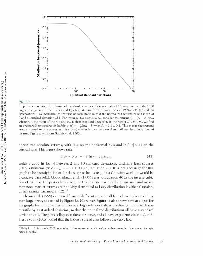
normalized absolute returns, with ln x on the horizontal axis and ln Pðjrj > xÞ on the

vertical axis. This figure shows that

ln Pðjrj > xÞ ¼ �zr ln xþ constant ð41Þyields a good fit for jrj between 2 and 80 standard deviations. Ordinary least squares

(OLS) estimation yields �zr ¼ �3:1� 0:1(i.e., Equation 40). It is not necessary for this

graph to be a straight line or for the slope to be �3 (e.g., in a Gaussian world, it would be

a concave parabola). Gopikrishnan et al. (1999) refer to Equation 40 as the inverse cubic

law of returns. The particular value zr ’ 3 is consistent with a finite variance and means

that stock market returns are not Levy distributed (a Levy distribution is either Gaussian,

or has infinite variance, zr52).27

Plerou et al. (1999) examined firms of different sizes. Small firms have higher volatility

than large firms, as verified by Figure 4a. Moreover, Figure 4a also shows similar slopes for

the graphs for four quartiles of firm size. Figure 4b normalizes the distribution of each size

quantile by its standard deviation, so that the normalized distributions all have a standard

deviation of 1. The plots collapse on the same curve, and all have exponents close to zr ’ 3.

Plerou et al. (2005) found that the bid-ask spread also follows the cubic law.

Figure 3

Empirical cumulative distribution of the absolute values of the normalized 15-min returns of the 1000

largest companies in the Trades and Quotes database for the 2-year period 1994–1995 (12 million

observations). We normalize the returns of each stock so that the normalized returns have a mean of0 and a standard deviation of 1. For instance, for a stock i, we consider the returns r

0it ¼ ðrit � riÞ=sr;i,

where ri is the mean of the rit’s and sr;i is their standard deviation. In the region 2 x 80, we find

an ordinary-least-squares fit lnPðjrj > xÞ ¼ �zr lnxþ b, with zr ¼ 3:1� 0:1. This means that returns

are distributed with a power law Pðjrj > xÞ ~x�zr for large x between 2 and 80 standard deviations ofreturns. Figure taken from Gabaix et al. 2003.

27Using Lux & Sornette’s (2002) reasoning, it also means that stock market crashes cannot be the outcome of simple

rational bubbles.

www.annualreviews.org � Power Laws in Economics and Finance 277

Ann

u. R

ev. E

con.

200

9.1.

Dow

nloa

ded

from

arj

ourn

als.

annu

alre

view

s.or

gby

NE

W Y

OR

K U

NIV

ER

SIT

Y -

BO

BST

LIB

RA

RY

on

08/1

1/09

. For

per

sona

l use

onl

y.

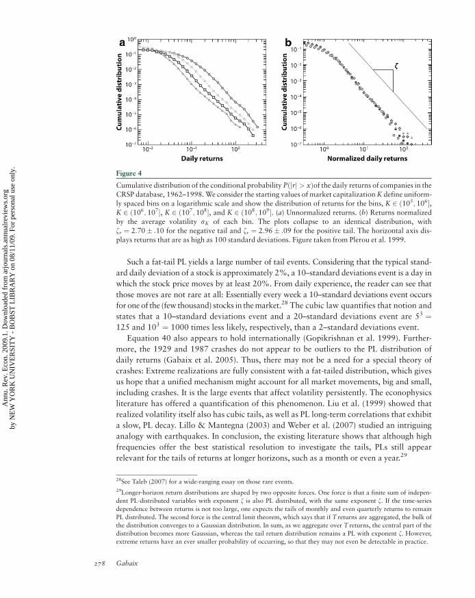
Such a fat-tail PL yields a large number of tail events. Considering that the typical stand-

ard daily deviation of a stock is approximately 2%, a 10–standard deviations event is a day in

which the stock price moves by at least 20%. From daily experience, the reader can see that

those moves are not rare at all: Essentially every week a 10–standard deviations event occurs

for oneof the (few thousand) stocks in themarket.28 The cubic law quantifies that notion and

states that a 10–standard deviations event and a 20–standard deviations event are 53 ¼125 and 103 ¼ 1000 times less likely, respectively, than a 2–standard deviations event.

Equation 40 also appears to hold internationally (Gopikrishnan et al. 1999). Further-

more, the 1929 and 1987 crashes do not appear to be outliers to the PL distribution of

daily returns (Gabaix et al. 2005). Thus, there may not be a need for a special theory of

crashes: Extreme realizations are fully consistent with a fat-tailed distribution, which gives

us hope that a unified mechanism might account for all market movements, big and small,

including crashes. It is the large events that affect volatility persistently. The econophysics

literature has offered a quantification of this phenomenon. Liu et al. (1999) showed that

realized volatility itself also has cubic tails, as well as PL long-term correlations that exhibit

a slow, PL decay. Lillo & Mantegna (2003) and Weber et al. (2007) studied an intriguing

analogy with earthquakes. In conclusion, the existing literature shows that although high

frequencies offer the best statistical resolution to investigate the tails, PLs still appear

relevant for the tails of returns at longer horizons, such as a month or even a year.29

Figure 4

Cumulative distribution of the conditional probability Pðjrj > xÞof the daily returns of companies in the

CRSP database, 1962–1998.We consider the starting values of market capitalizationK define uniform-ly spaced bins on a logarithmic scale and show the distribution of returns for the bins, K 2 ð105; 106�,K 2 ð106; 107�, K 2 ð107; 108�, and K 2 ð108; 109�. (a) Unnormalized returns. (b) Returns normalized

by the average volatility sK of each bin. The plots collapse to an identical distribution, with

zr ¼ 2:70� :10 for the negative tail and zr ¼ 2:96� :09 for the positive tail. The horizontal axis dis-plays returns that are as high as 100 standard deviations. Figure taken from Plerou et al. 1999.

28See Taleb (2007) for a wide-ranging essay on those rare events.

29Longer-horizon return distributions are shaped by two opposite forces. One force is that a finite sum of indepen-

dent PL-distributed variables with exponent z is also PL distributed, with the same exponent z. If the time-series

dependence between returns is not too large, one expects the tails of monthly and even quarterly returns to remain

PL distributed. The second force is the central limit theorem, which says that if T returns are aggregated, the bulk of

the distribution converges to a Gaussian distribution. In sum, as we aggregate over T returns, the central part of the

distribution becomes more Gaussian, whereas the tail return distribution remains a PL with exponent z. However,

extreme returns have an ever smaller probability of occurring, so that they may not even be detectable in practice.

278 Gabaix

Ann

u. R

ev. E

con.

200

9.1.

Dow

nloa

ded

from

arj

ourn

als.

annu

alre

view

s.or

gby

NE

W Y

OR

K U

NIV

ER

SIT

Y -

BO

BST

LIB

RA

RY

on

08/1

1/09

. For

per

sona

l use

onl

y.

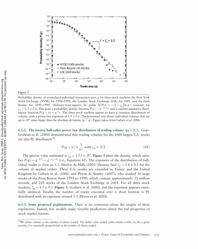
6.1.2. The inverse half-cubic power law distribution of trading volume: zq’ 3=2. Gopi-

krishnan et al. (2000) demonstrated that trading volumes for the 1000 largest U.S. stocks

are also PL distributed:30

Pðq > xÞ / 1

xzqwith zq ’ 3=2: ð42Þ

The precise value estimated is zq ¼ 1:53� :07. Figure 5 plots the density, which satis-

fies PðqÞ � q�2:5 ¼ q�ðzqþ1Þ (i.e., Equation 42). The exponent of the distribution of indi-

vidual trades is close to 1:5. Maslov & Mills (2001) likewise find zq ¼ 1:4� 0:1 for the

volume of market orders. These U.S. results are extended to France and the United

Kingdom by Gabaix et al. (2006) and Plerou & Stanley (2007), who studied 30 large

stocks of the Paris Bourse from 1995 to 1999, which contain approximately 35 million

records, and 250 stocks of the London Stock Exchange in 2001. For all three stock

markets, zq ¼ 1:5� 0:1 (Figure 5) (Gabaix et al. 2006), and the exponent appears essen-

tially identical. Finally, the number of trades executed over a short horizon is PL

distributed with an exponent around 3.3 (Plerou et al. 2000).

6.1.3. Some proposed pxplanations. There is no consensus about the origins of these

regularities. Indeed, few models make testable predictions about the tail properties of

stock market returns.

Figure 5

Probability density of normalized individual transaction sizes q for three stock markets: the New York

Stock Exchange (NYSE) for 1994–1995, the London Stock Exchange (LSE) for 2001, and the Paris

Bourse for 1995–1999. Ordinary-least-squares fit yields ln PðxÞ ¼ �ð1þ zq�ln xþ constant for

zq ¼ 1:5� 0:1. This gives a probability density function PðxÞ � x�ð1þzqÞ and a countercumulative distri-

bution function Pðq > xÞ � x�zq . The three stock markets appear to have a common distribution of

volume, with a power law exponent of 1:5� 0:1. The horizontal axis shows individual volumes that are

up to 104 times larger than the absolute deviation, jq� q� j�. Figure taken from Gabaix et al. 2006.

30We define volume as the number of shares traded. The dollar value traded yields similar results, as, for a given

security, it is essentially proportional to the number of shares traded.

www.annualreviews.org � Power Laws in Economics and Finance 279

Ann

u. R

ev. E

con.

200

9.1.

Dow

nloa

ded

from

arj

ourn

als.

annu

alre

view

s.or

gby

NE

W Y

OR

K U

NIV

ER

SIT

Y -

BO

BST

LIB

RA

RY

on

08/1

1/09

. For

per

sona

l use

onl

y.

The fat tail of returns could come from ARCH effects, as discussed in Section 3.3. It

would be nice to have an economic model that generates such dynamics, perhaps via a

feedback rule, or the dynamics of liquidity. Ideally, it would simultaneously explain the

cubic and half-cubic laws of stock market activity. However, this model does not appear to

have been written yet.

Another model, proposed by Gabaix et al. (2003, 2006), attributes the PLs of

trading activity to the strategic trades of very large institutional investors in relatively

illiquid markets. This activity creates spikes in returns and volume, even in the absence of

important news about fundamentals, and generates the cubic and half-cubic laws. Ante-

cedents of this model include Levy & Solomon (1996), who expressed that large traders

have a large price impact and predicted zr ¼ zS (see Levy 2005 for some evidence in

that direction). Solomon & Richmond (2001) proposed an amended theory, predic-

ting zr ¼ 2zS. In Gabaix et al.’s model, cost-benefit considerations lead to zr ¼ 3zS, asshown below.

Examples of this mechanism may include the crash of Long Term Capital Manage-

ment in the summer of 1998, the rapid unwinding of very large stock positions by

Societe Generale after the Kerviel rogue trader scandal (which led stock markets to fall,

and the Fed to cut interest rates by 75 basis points on January 22, 2008), the conjec-

ture by Khandani & Lo (2007) that one large fund was responsible for the crash of

quantitative funds in August 2007, and even the crash of 1987 (see the discussion in

Gabaix et al. 2006). Of course, such a theory may at most be a theory of the impulse.

The dynamics of the propagation are left for future research. According to the PL

hypothesis, these types of actions happen at all timescales, including small ones, such

as day to day.

Gabaix et al.’s (2006) theory works the following way. For example, let us suppose that

a trade of size q generates a percentage price impact equal to kqg, for a constant g (Gabaix

et al. 2006 present a microfoundation for g ¼ 1=2). A mutual fund would not want to lose

more than a certain percentage of returns in price impact (because the trader wants his

trading strategy to be robust to model uncertainty). Each trade costs its dollar value q

times the price impact, hence kq1þg dollars. Optimally, the fund trades as much as possi-

ble, subject to the robustness constraint. That implies kq1þg / S; hence the typical trade

of a fund of size S is of volume q / S1=ð1þgÞ, and its typical price impact is

jDpj ¼ kqg / Sg=ð1þgÞ. (Those predictions await empirical testing with microdata.) Using

rule 4, this generates the following PL exponents for returns and volumes:

zr ¼ 1þ 1

g

� �zS; zg ¼ ð1þ gÞzS: ð43Þ

Hence the theory links the PL exponents of returns and trades to the PL exponent of

mutual-fund sizes and price impact. Given the finding of a Zipf distribution of fund sizes

(zS ¼ 1, which presumably comes from the random growth of funds), and a square-root

price impact (g ¼ 1=2Þ, we obtain zr ¼ 3 and zq ¼ 3=2, the empirically found exponents of

returns and volumes.

6.2. Other Scaling in Finance

Wyart et al. (2008) offered a simple, original theory of the bid-ask spread, which yields a

new empirical prediction:

280 Gabaix

Ann

u. R

ev. E

con.

200

9.1.

Dow

nloa

ded

from

arj

ourn

als.

annu

alre

view

s.or

gby

NE

W Y

OR

K U

NIV

ER

SIT

Y -

BO

BST

LIB

RA

RY

on

08/1

1/09

. For

per

sona

l use

onl

y.

Ask� Bid

Price¼ k

sffiffiffiffiffiN

p ; ð44Þ

where s is the daily volatility of the stock, N is the average number of trades for the stock,

and k is a constant (in practice roughly close to 1). They found good support for this

prediction, which has the following basic reasoning (their model has more sophisticated

variants). We suppose that at each trade, the log price moves by k�1 times the bid-ask

spread S. After N trades, assumed to have independent signs, the standard deviation of the

log price move is k�1SffiffiffiffiffiN

p. This should be the daily price move, so k�1KS

ffiffiffiffiffiN

p ¼ s, henceEquation 44. Of course, some of the microfoundations remain unclear, but at least we

have a simple new hypothesis, which makes a good scaling prediction and has empirical

support. Bouchaud & Potters (2004) and Bouchaud et al. (2009) provide good sources on

scaling in finance, particularly in microstructure.

In another example in finance, during stock market bubbles, it is plausible that some

stocks are particularly overvalued. Hence, the size distribution of stock is more skewed, as

shown by various authors (Kou & Kou 2004, Kaizoji 2006). It would be nice to know if

this skewness offers a useful predictive complement to the more traditional measures, such

as the ratio of market value to book value.

6.3. International Trade

In an important new result, Hinloopen & van Marrewijk (2008) demonstrated that the

Balassa index of revealed comparative advantage satisfies Zipf’s law. Moreover, the size

distribution of exporters might be roughly Zipf (see figure 3 in Helpman et al. 2004).31

However, previous models explain a PL of the size of exporters (Arkolakis 2008, Chaney

2008, Melitz 2003) but not why the exponent should be approximately 1. Presumably,

this literature will import some ideas from the firm-size literature to identify the root

causes of the Zipf feature of exports (see Eaton et al. 2004 for a study of many PLs in the

fine structure of exports).

6.4. Other Candidate Laws

Mulligan & Shleifer (2004) established another candidate law in the supply of regulations.

In the United States, the quantity of regulations (as measured by the number of lines of

text) is proportional to the square root of each state’s population. Mulligan & Shleifer

provide an efficiency-based explanation for this phenomenon. It would be interesting to

investigate their findings outside the United States.

Edmans et al. (2009) studied a model with multiplicative preferences and multiplicative

actions for CEO incentives: At the margin, if the CEO works 1% more, the firm value

increases by a given percentage, and his utility (expressed in consumption-equivalent

terms) decreases by a another percentage. This predicts the following structure for incen-

tives. For a given percentage firm return d ln S, there should be a proportional percentage

increase in the CEO’s pay d lnw ¼ b�d ln S, for a coefficient b independent of size. This

prediction of size-independence holds true empirically. Also, such a relation could not

31In that figure, the standard errors are too narrow because the authors use the OLS standard errors, which have a

large downward bias. See Section 7 for the correct standard errors, z ð2=NÞ1=2.

www.annualreviews.org � Power Laws in Economics and Finance 281

Ann

u. R

ev. E

con.

200

9.1.

Dow

nloa

ded

from

arj

ourn

als.

annu

alre

view

s.or

gby

NE

W Y

OR

K U

NIV

ER

SIT

Y -

BO

BST

LIB

RA

RY

on

08/1

1/09

. For

per

sona

l use

onl

y.

hold with a nonmultiplicative traditional utility function.32 The scaling of incentives with

respect to firm size tells us a great deal about the economic nature of the incentive

problem.

From this, it is easy to predict the value of Jensen & Murphy’s (1990) measure of

incentives dw=dS, i.e., by how many dollars the CEO pay changes, for a given dollar change

in firm value. Jensen & Murphy estimated that it was approximately 3/1000 and suggested

that this result meant that incentives are too weak. However, Edmans et al.’s (2009) model

shows that it should optimally be dw=dS ¼bw=S. Hence, it should be very small in practice

(as the wage is of the order of magnitude of a few million dollars, and the firm size a few

billion dollars, so w=S is of the order of magnitude of one-thousandth), which explains

Jensen & Murphy’s finding. Furthermore, as seen in Section 5.5, CEO wage is proportional

to S1=3. Therefore, the model predicts that the Jensen-Murphy incentive bw=S should scale

as S�2=3. This relationship holds empirically in the United States. As with the above case,

it would be nice to investigate these predictions outside the United States.

Empirical networks are also full of PLs (see Jackson 2009, Newman et al. 2006). For

instance, on the Internet, some Web pages are popular, with many pages linking to them,

whereas most pages are not so popular. The number of links to a certain Web page follows

a PL distribution. Most models of networks build on Simon’s (1955) model. Finally, we

mention that Johnson et al. (2006) found that the number of deaths in armed conflicts

follows a PL, with an exponent around 2.5, and provide a model for it.

6.5. Power Laws Outside of Economics

Ever since Zipf (1949), the popularity of words has been found to follow Zipf’s law,33 yet

there is no consensus on the origin of that regularity. One explanation might be Simon’s

(1955) model or more recent models based on Champernowne (1953). Another might be

the “monkeys at the typewriter” model (reprinted in Mandelbrot 1997, p. 225, originally

written by the same author in 1951). A monkey types randomly on a typewriter (each of n

letters being hit with probability q=nÞ, and there is a new word when he hits the space bar

(which happens with probability 1� q). After 1 billion hours, we count the word frequen-

cy. This simple exercise yields a PL for the word distribution, with exponent

z ¼ 1=ð1� ln q=ln nÞ[because each of the nk words with length k has frequency

ð1� qÞðq=nÞk]. When the space bar is hit with low probability, or the number of letters

gets large, the exponent becomes close to 1. This argument, although interesting, is not

dispositive. It might be that the Zipf distribution of word use corresponds to a maximal

efficiency of the use of concepts (in that direction, see Mandelbrot 1953, which uses

entropy maximization, and Carlson & Doyle 1999). Perhaps our minds need to use a

hierarchy of concepts, which follows Zipf’s law. This would make Zipf’s law much more

linguistically and cognitively relevant. In that vein, Chevalier & Goolsbee (2003) noted a

roughly Zipf distribution of book sale volume at online retailers [although a different

methodology by Deschastres & Sornette (2005) gives an exponent around 2]. This may

be because of random growth, or perhaps because, similar to words, the good ideas follow

32It must be possible to write the utility function uðcfðeÞÞ, where c is consumption and e is effort, which is precisely

the form typically used in macroeconomics. A generic function uðcÞ � fðeÞ, typically used in incentive theory, would

predict the incorrect scaling of incentive with respect to size.

33Interestingly, McCowan et al. (1999) showed that Zipf’s law is not limited to human language: It also holds for

dolphins.

282 Gabaix

Ann

u. R

ev. E

con.

200

9.1.

Dow

nloa

ded

from

arj

ourn

als.

annu

alre

view

s.or

gby

NE

W Y

OR

K U

NIV

ER

SIT

Y -

BO

BST

LIB

RA

RY

on

08/1

1/09

. For

per

sona

l use

onl

y.

a PL distribution. Similarly, De Vany (2003) showed many fat tails in the movie industry,

and Kortum (1997) proposed a model of research delivering a PL distribution of ideas.

PLs are also of significant interest outside of economics. In biology, there is a surpris-

ingly large number of PL regularities, referred to as allometric scaling. For instance, the

energy that an animal of mass M requires to live is proportional to M3=4. This empirical

regularity, expressed in Figure 6, has been explained only recently by West et al. (1997)

along the following lines: If one wants to design an optimal vascular system to send

nutrients to the animal, one designs a fractal system, and maximum efficiency exactly

delivers the M3=4 law. In explaining the relationship between energy needs and mass, one

should not become distracted by thinking about the specific features of animals, such as

feathers and fur. Simple and deep principles underlie the regularities.

Explaining and understanding PL exponents compose a large part of the theory of

critical phenomena in physics (e.g., Stanley 1999). For example, heating a magnet lowers

its magnetism, up to a critical temperature, at which the magnetism entirely disappears;

right below the critical temperature Tc, the strength of the magnet is ðTc � TÞa for some

exponent a. Different materials behave identically around a critical point, a phenomenon

reminiscent of universality. Finally, PLs occur in a range of natural phenomena, including

earthquakes (Sornette 2004), forest fires (Malamud et al. 1998), and many other events.

Figure 6

Metabolic rate for a series of mammals and birds as a function of mass. The scale is logarithmic, and

the slope of 3=4 exemplifies Kleiber’s law: The metabolic rate of an animal of mass m is proportional

to m3=4. This law has recently been explained by West et al. 1997. Figure taken from West et al. 2000.

www.annualreviews.org � Power Laws in Economics and Finance 283

Ann

u. R

ev. E

con.

200

9.1.

Dow

nloa

ded

from

arj

ourn

als.

annu

alre

view

s.or

gby

NE

W Y

OR

K U

NIV

ER

SIT

Y -

BO

BST

LIB

RA

RY

on

08/1

1/09

. For

per

sona

l use

onl

y.

7. ESTIMATION OF POWER LAWS

7.1. Estimating

To illustrate how one estimates a distributional PL, we take the example of cities. We

order cities by size Sð1Þ � . . .� SðnÞ, stopping at a rank n, which is a cutoff still in the upper

tail. However, there is not a consensus on how to pick the optimal cutoff (see Beirlant

et al. 2004). Most applied researchers indeed rely on a visual goodness of fit to select the

cutoff or use a simple rule, such as choosing all the observations in the top 5% of the

distribution. Systematic procedures require the econometrician to estimate further param-

eters (Embrechts et al. 1997), and none has gained widespread use. Given the number of

points in the upper tail, there are two main methods of estimation.34 The first method is

Hill’s (1975) estimator:

BHill ¼ ðn� 2Þ=Xn�1

i¼1

�ln SðiÞ � ln SðnÞ

�; ð45Þ

which has35 a standard error BHillðn� 3Þ�1=2. The second method is a log-rank, log-size

regression, in which B is the slope in the regression of the log rank i on the log size:

lnði� sÞ ¼ constant� BOLS lnSðiÞ þ noise: ð46Þ

This estimate has an asymptotic standard error BOLSðn=2Þ�1=2 (the standard error

returned by OLS software is wrong because the ranking procedure makes the residuals

positively autocorrelated). A shift s ¼ 0 has been typically used, but a shift s ¼ 1=2 is

optimal to reduce the small-sample bias, as Gabaix & Ibragimov (2008a) have shown.

The OLS method is typically more robust to deviations from PLs than the Hill

estimator.

This log-log regression can be heuristically justified as follows. Let us suppose that size

S follows a PL with countercumulative distribution function kS�z. We draw n� 1 units

from that distribution and order them Sð1Þ � ::: � Sðn�1Þ. Then,36 we have i=n ¼ E½kS�z

ðiÞ �,which motivates the following approximate statement:

Rank ’ nk Size�z: ð47ÞSuch a statement is sometimes referred to as rank-size rule. We note that even if the PL fits

exactly, the rank-size rule (Equation 47) is only approximate. But it does at least offer

some motivation for the empirical specification (Equation 46).

Both methods have pitfalls, and the true errors are often bigger than the nominal

standard errors, as discussed by Embrechts et al. (1997, pp. 330–45). Indeed, in many

data sets (particularly in finance), observations are not independent. For instance, it is

34A basic theoretical tool is the Renyi representation theorem: For i5n, the differences lnSðiÞ � lnSðnÞ have jointly

the distribution of the sums z�1Pn�1k¼i Xk=k, where the Xk are independent draws of a standard exponential distribu-

tion PðXk > xÞ ¼ e�x for x � 0.

35Much of the literature estimates 1=z rather than z, hence the n� 2 and n� 3 factors here, rather than the usual n.

I have been unable to find an earlier reference for those expressions, so I derived them for this review. It is easy to

show that they are the correct ones to get unbiased estimates, using the Renyi theorem, and the fact that

X1 þ :::þXn has density xn�1e�x=ðn� 1Þ! when xi are independent draws from a standard exponential distribution.

36This is if S has countercumulative function FðxÞ; then FðSÞ follows a standard uniform distribution, and the

expectation of the i-th smallest value out of n� 1 of a uniform distribution is i=n.

284 Gabaix

Ann

u. R

ev. E

con.

200

9.1.

Dow

nloa

ded

from

arj

ourn

als.

annu

alre

view

s.or

gby

NE

W Y

OR

K U

NIV

ER

SIT

Y -

BO

BST

LIB

RA

RY

on

08/1

1/09

. For

per

sona

l use

onl

y.

economically accepted that many extreme stock market returns are clustered in time

and affected by the same factors. Hence, standard errors will be illusorily too low if

one assumes that the data are independent. There is no consensus procedure to over-

come that problem. In practice, applied papers often report the Hill or OLS estimator,

together with a caveat that the observations are not necessarily independent, so that the

nominal standard errors probably underestimate the true standard errors. Moreover,

sometimes a lognormal fits better. Indeed, since early on, some have attacked the fit

of the Pareto law (see Persky 1992). The reason, broadly, is that adding more param-

eters (e.g., a curvature), as a lognormal permits, can only improve the fit. However,

the Pareto law has survived the test of time: It fits still quite well. The extra degree

of freedom allowed by a lognormal might be a distraction from the essence of the

phenomenon.

7.2. Testing

With an infinitely large empirical data set, one can reject any nontautological theory.

Hence, the main question of empirical work should be how well a theory fits, rather than

whether it fits perfectly (i.e., within the standard errors). Leamer & Levinsohn (1995)

argue that, in the context of empirical research in international trade, too much energy is

spent seeing if a theory fits exactly. Rather, researchers should aim at broad, although

necessarily nonabsolute, regularities. In other words, “estimate, don’t test.”

Iriji & Simon (1964, p. 78) remarked that Galileo’s law of the inclined plane, which

states that the distance traveled by a ball rolling down the plane increases with the square

of the time,

does ignore variables that may be important under various circumstances:

irregularities in the ball or the plane, rolling friction, air resistance, possible

electrical or magnetic fields if the ball is metal, variations in the gravitational

field and so on, ad infinitum. The enormous progress that physics has made in

three centuries may be partly attributed to its willingness to ignore for a time

discrepancies from theories that are in some sense substantially correct.

Consistent with these suggestions, some of the debate on Zipf’s law should be cast in

terms of how well, or poorly, it fits, rather than whether it can be rejected. The empirical

research establishes that the data are typically well described by a PL with exponent

z 2 ½0:8; 1:2�: This pattern catalyzes a search for an underlying mechanism.

Nonetheless, it is useful to have a test, so what is a test for the fit of a PL? Many papers

in practice do not provide such a test. Some authors (Clauset et al. 2008) advocate the

Kolmogorov-Smirnov test. Gabaix & Ibragimov (2008b) provided a simple test using the

OLS regression framework of the previous subsection. We define s �cov

�ðln SjÞ2; ln Sj

�2varðln SjÞ and

run the OLS regression,

ln i� 1

2

� �¼ constant� B lnSðiÞ þ q

�ln SðiÞ � s

�2

þ noise; ð48Þ

to estimate the values B and q. The term ðlnSi � sÞ2 captures a quadratic deviation from

an exact PL, and the coefficient s recenters the quadratic term. With this recentering,

the estimate of the PL exponents B is the same regardless of the inclusion of the quad-

www.annualreviews.org � Power Laws in Economics and Finance 285

Ann

u. R

ev. E

con.

200

9.1.

Dow

nloa

ded

from

arj

ourn

als.

annu

alre

view

s.or

gby

NE

W Y

OR

K U

NIV

ER

SIT

Y -

BO

BST

LIB

RA

RY

on

08/1

1/09

. For

per

sona

l use

onl

y.

ratic term. The test of the PL is to reject the null of an exact PL if and only if

j q =B2j > 1:95�ð2nÞ�1=2.

8. CONCLUSION

As the history of science shows, trying to solve apparently narrow, but sharply posed,

nontrivial problems is a fruitful way to make substantial progress. As Schumpeter (1949,

p. 155) noted for PLs, studying such questions may “lay the foundations for an entirely

novel type of theory.” PLs have forced economists to write new theories, e.g., on the

origins of cities, firms, international trade, CEO pay, or of extreme movements in stock

market fluctuations. Accordingly, I list some open questions in the Future Issues section.

The time is ripe for economists to use those PLs to investigate old and new regularities

with renewed models and data, continuing the tradition of Gibrat, Champernowne,

Mandelbrot, and Simon.

FUTURE ISSUES

Theory

1. Is there a deep explanation for the coefficient of 1=3 capital share in the aggre-

gate capital stock? This constancy is one of the most remarkable regularities in

economics. A fully satisfactory explanation should not only generate the con-

stant capital share, but some reason why the exponent should be 1=3 (see Jones

2005 for an interesting paper that generates a Cobb-Douglas production func-

tion, but does not predict the 1=3 exponent). With such an answer, we might

understand more deeply what causes technological progress and the foundations

of economic growth.

2. Can we fully explain the PL distribution of financial variables, particularly returns

and trading volume? The theories sketched above are at best partial. Working out a

full theory of large financial movements, guided by PLs, might, surprisingly, be key

to the explanation of both excess volatility and financial crashes and may perhaps

inform appropriate risk-management or policy responses.

3. Is there an explanation for the PL distribution of firms that is not based on a

simple mechanical Gibrat’s law, but instead comes from efficiency maximiza-

tion? For instance, in biology, PLs maximize physiological efficiency (West et al.

1997). An organism with a scale-free (fractal) organization is optimal under

many circumstances. It is plausible that the same property arises in economics.

Of course, the same may hold for Zipf’s law for words. It might be the case that

the Zipf distribution of word frequency corresponds to a maximal efficiency of

the use of concepts.

4. Is there a deep explanation for the coefficient of 1/3 in the Roberts’ law listed

in Section 5.5? Some theories predict a relation w / Sk, for some k between

0 and 1, but none predicts why the exponent should be (roughly) 1/3. Gabaix &

Landier (2008) show that the exponent 1/3 arises if the distribution of talents has

a square-root-shaped upper bound. Is there any natural mechanism, perhaps

random growth for the accumulation or detection of talent, that would generate

286 Gabaix

Ann

u. R

ev. E

con.

200

9.1.

Dow

nloa

ded

from

arj

ourn

als.

annu

alre

view

s.or

gby

NE

W Y

OR

K U

NIV

ER

SIT

Y -

BO

BST

LIB

RA

RY

on

08/1

1/09

. For

per

sona

l use

onl

y.

that distribution? With such an insight, we might understand better how top

talent (which may be a crucial engine in growth) is accumulated.

5. Is there a way to generate macroeconomic fluctuations purely from microeco-

nomic shocks? Bak et al. (1993) suggested a rather fascinating possibility, in

which inventory needs propagate throughout the economy (Nirei 2006 is a

related model). Those models have not convinced economists, as they do not

make tight predictions and tend to generate fluctuations with tails that are too

fat (they are Levy distributions with infinite variance). Still, they might be on the

right track. Gabaix (2007)’s theory of granular fluctuations generates fluctuations

from the existence of large firms or sectors (see also Brock & Durlauf 2001,

Durlauf 1993). These models are still hypotheses [although di Giovanni & Lev-

chenko (2009) represent promising progress]. Better understanding of the origins

of macroeconomic fluctuations should lead to better models and policies.

Empirics

6. Do tail events matter for investors, in particular for risk premia? Various authors

have argued that they do (Barro 2006, Gabaix 2008, Ibragimov et al. 2009,

Weitzman 2007), and this is a subject of ongoing research.

7. Can we test superstar models (Gabaix & Landier 2008, Rosen 1981) to see if the

link among stakes (e.g., advertising revenues), talents (e.g., the ability of a golf-

er), and income is predicted by these theories? In addition, comparing the ex-

treme in the perceptions of talent across different fields might lead to surprising

similarities between those fields.

8. With the availability of large new data sets to test models’ predictions about

microeconomic behavior, what new PLs will be discovered?

DISCLOSURE STATEMENT

The author is not aware of any affiliations, memberships, funding, or financial holdings

that might be perceived as affecting the objectivity of this review.

ACKNOWLEDGMENTS

This work was supported by NSF grant 0527518. I thank Esben Hedegaard and Rob

Tumarkin for very good research assistance, Jonathan Parker for the Schumpeter quota-

tion, and Alex Edmans, Parameswaran Gopikrishnan, Chad Jones, David Laibson, Moshe

Levy, Sorin Solomon, and Gene Stanley for helpful comments.

LITERATURE CITED

Acemoglu D, Cao D. 2009. Innovation by entrants and incumbents. Work. Pap., Mass. Inst. Technol.

Amaral LAN, Buldyrev SV, Havlin S, Leschhorn H, Maass P, et al. 1997. Scaling behavior in econom-

ics: I. Empirical results for company growth. J. Phys. (France) I 7:621–33

www.annualreviews.org � Power Laws in Economics and Finance 287

Ann

u. R

ev. E

con.

200

9.1.

Dow

nloa

ded

from

arj

ourn

als.

annu

alre

view

s.or

gby

NE

W Y

OR

K U

NIV

ER

SIT

Y -

BO

BST

LIB

RA

RY

on

08/1

1/09

. For

per

sona

l use

onl

y.

Arkolakis C. 2008. Market penetration costs and trade dynamics. Work. Pap., Dept. Econ., Yale

Univ.

Atkinson AB, Piketty T. 2007. Top Incomes over the Twentieth Century. Oxford, UK: Oxford Univ.

Press

Audretsch DB, Klomp L, Santarelli E, Thurik AR. 2004. Gibrat’s law: Are the services different? Rev.

Industr. Org. 24:301–24

Auerbach F. 1913. Das Gesetz der Bevolkerungskonzentration. Petermanns Geogr. Mitt. 59:74–76

Axtell R. 2001. Zipf distribution of U.S. firm sizes. Science 293:1818–20

Bak P, Chen K, Woodford M. 1993. Aggregate fluctuations from independent sectoral shocks:

self-organized criticality in a model of production and inventory dynamics. Ric. Econ. 47:

3–30

Baker G, Jensen M, Murphy K. 1988. Compensation and incentives: practice vs. theory. J. Financ.

43:593–616

Barabasi AL, Albert R. 1999. Emergence of scaling in random networks. Science 286:509–12

Barro J, Barro RJ. 1990. Pay, performance, and turnover of bank CEOs. J. Labor Econ. 8:448–81

Barro RJ. 2006. Rare disasters and asset markets in the twentieth century. Q. J. Econ. 121:823–66

Beirlant J, Goegebeur Y, Segers J, Teugels J. 2004. Statistics of Extremes Theory and Applications.

Chichester, UK: Wiley

Benguigui L, Blumenfeld-Lieberthal E. 2007. A dynamic model for city size distribution beyond Zipf’s

law. Phys. A 384:613–27

Benhabib J, Bisin A. 2007. The distribution of wealth: intergenerational transmission and redistribu-

tive policies. Work. Pap., New York Univ.

Biggs M. 2005. Strikes as forest fires: Chicago and Paris in the late nineteenth century. Am. J. Sociol.

110:1684–714

Bouchaud JP. 2001. Powerlaws in economics and finance: some ideas from physics. Quant. Fin.

1:105–12

Bouchaud JP, Farmer JD, Lillo F. 2009. How markets slowly digest changes in supply and demand.

In Handbook of Financial Markets: Dynamics and Evolution, ed. T Hens, KR Schenkhoppe,

pp. 57–130. Amsterdam: Elsevier

Bouchaud JP, Potters M. 2004. Theory of Financial Risk and Derivative Pricing: From Statistical

Physics to Risk Management. Cambridge, UK: Cambridge Univ. Press

Brakman S, Garretsen H, van Marrewijk C. 2009. A New Introduction to Geographical Economics.

Cambridge, UK: Cambridge Univ. Press. 2nd ed.

Brock W, Durlauf S. 2001. Discrete choice with social interactions. Rev. Econ. Stud. 68:235–60

Carlson JM, Doyle J. 1999. Highly optimized tolerance: a mechanism for power laws in designed

systems. Phys. Rev. E 60:1412–27

Carroll G. 1982. National city-size distributions: What do we know after 67 years of research? Prog.

Hum. Geogr. 6:1–43

Carvalho V. 2008. Aggregate fluctuations and the network structure of intersectoral trade. Work.

Pap., Univ. of Chicago

Challet D, Marsili M, Zhang YC. 2005. Minority Games: Interacting Agents in Financial Markets.

Oxford, UK: Oxford Univ. Press

Champernowne D. 1953. A model of income distribution. Econ. J. 83:318–51

Chaney T. 2008. Distorted gravity: the intensive and extensive margins of international trade. Am.

Econ. Rev. 98:1707–21

Chevalier J, Goolsbee A. 2003. Measuring prices and price competition online: Amazon and Barnes

and Noble. Quant. Mark. Econ. 1:203–22

Clauset A, Shalizi CR, Newman MEJ. 2008. Power-law distributions in empirical data. Work. Pap.,

Santa Fe Inst.

Cordoba J. 2008. On the distribution of city sizes. J. Urban Econ. 63:177–97

Cosh A. 1975. The remuneration of chief executives in the United Kingdom. Econ. J. 85:75–94

288 Gabaix

Ann

u. R

ev. E

con.

200

9.1.

Dow

nloa

ded

from

arj

ourn

als.

annu

alre

view

s.or

gby

NE

W Y

OR

K U

NIV

ER

SIT

Y -

BO

BST

LIB

RA

RY

on

08/1

1/09

. For

per

sona

l use

onl

y.

Deschatres F, Sornette D. 2005. The dynamics of book sales: endogenous versus exogenous shocks in

complex networks. Phys. Rev. E 72:016112

De Vany A. 2003. Hollywood Economics. New York: Routledge

di Giovanni J, Levchenko A. 2009. International trade and aggregate fluctuations in granular econo-

mies. Work. Pap., Univ. of Mich.

Di Guilmi C, Aoyama H, Gallegati M, Souma W. 2004. Do Pareto–Zipf and Gibrat laws hold true?

An analysis with European firms. Phys. A 335:197–216

Dragulescu A, Yakovenko VM. 2001. Evidence for the exponential distribution of income in the USA.

Eur. Phys. J. B 20:585–89

Duranton G. 2006. Some foundations for Zipf ’s law: product proliferation and local spillovers. Reg.

Sci. Urban Econ. 36:542–63

Duranton G. 2007. Urban evolutions: the fast, the slow, and the still. Am. Econ. Rev. 97:197–221

Durlauf S. 1993. Nonergodic economic growth. Rev. Econ. Stud. 60:349–66

Durlauf S. 2005. Complexity and empirical economics. Econ. J. 115:F225–43

Eaton J, Kortum S, Kramarz F. 2004. Dissecting trade: firms, industries, and export destinations.

Am. Econ. Rev. Pap. Proc. 94:150–54

Edmans A, Gabaix X, Landier A. 2009. A multiplicative model of optimal CEO incentives in market

equilibrium. Rev. Financ. Stud. In press

Eeckhout J. 2004. Gibrat’s law for (all) cities. Am. Econ. Rev. 94:1429–51

Embrechts P, Kluppelberg C, Mikosch T. 1997. Modelling Extremal Events for Insurance and

Finance. New York: Springer

Estoup JB. 1916. Les gammes stenographiques. Paris: Inst. Stenogr.

Fama E. 1963. Mandelbrot and the stable Paretian hypothesis. J. Bus. 36:420–29

Frydman C, Saks R. 2007. Historical trends in executive compensation, 1936-2003, Work. Pap.,

Harvard Univ.

Fu D, Pammolli F, Buldyrev SV, Riccaboni M, Matia K, et al. 2005. The growth of business firms:

theoretical framework and empirical evidence. Proc. Natl. Acad. Sci. USA 102:18801–6

Fujiwara Y. 2004. Zipf law in firms bankruptcy. Phys. A 337:219–30

Gabaix X. 1999a. Zipf’s law for cities: an explanation. Q. J. Econ. 114:739–67

Gabaix X. 1999b. Zipf’s law and the growth of cities. Am. Econ. Rev. Pap. Proc. 89:129–32

Gabaix X. 2007. The granular origins of aggregate fluctuations. Work. Pap., New York Univ.

Gabaix X. 2008. Variable rare disasters: a tractable framework for ten puzzles in macro-finance.

Work. Pap., New York Univ.

Gabaix X, Gopikrishnan P, Plerou V, Stanley HE. 2003. A theory of power law distributions in

financial market fluctuations. Nature 423:267–70

Gabaix X, Gopikrishnan P, Plerou V, Stanley HE. 2005. Are stock market crashes outliers? Work.

Pap., Mass. Inst. Technol.

Gabaix X, Gopikrishnan P, Plerou V, Stanley HE. 2006. Institutional investors and stock market

volatility. Q. J. Econ. 121:461–504

Gabaix X, Ibragimov R. 2008a. Rank-1/2: a simple way to improve the OLS estimation of tail

exponents. Work Pap., NBER

Gabaix X, Ibragimov R. 2008b. A simple OLS test of power law behavior. Work. Pap., Harvard

Univ.

Gabaix X, Ioannides Y. 2004. The evolution of the city size distributions. In Handbook of Regional

and Urban Economics, ed. Henderson V, Thisse JF, 4:2341–78. Oxford: Elsevier

Gabaix X, Landier A. 2008. Why has CEO pay increased so much? Q. J. Econ. 123:49–100

Gibrat R. 1931. Les Inegalites Economiques. Paris: Libr. Recl. Sirey

Gopikrishnan P, Gabaix X, Plerou V, Stanley HE. 2000. Statistical properties of share volume traded

in financial markets. Phys. Rev. E 62:R4493–96

Gopikrishnan P, Plerou V, Amaral L, Meyer M, Stanley HE. 1999. Scaling of the distribution of

fluctuations of financial market indices. Phys. Rev. E 60:5305–16

www.annualreviews.org � Power Laws in Economics and Finance 289

Ann

u. R

ev. E

con.

200

9.1.

Dow

nloa

ded

from

arj

ourn

als.

annu

alre

view

s.or

gby

NE

W Y

OR

K U

NIV

ER

SIT

Y -

BO

BST

LIB

RA

RY

on

08/1

1/09

. For

per

sona

l use

onl

y.

Goldie CM. 1991. Implicit renewal theory and tails of solutions of random equations. Ann. Appl.

Probab. 1:126–66

Helpman E, Melitz MJ, Yeaple SR. 2004. Export versus FDI with heterogeneous firms. Am. Econ.

Rev. 94:300–16

Hill BM. 1975. A simple approach to inference about the tail of a distribution. Ann. Stat. 3:1163–74

Hinloopen J, van Marrewijk C. 2008. Comparative advantage, the rank-size rule, and Zipf’s law.

Work. Pap., Tinbergen Inst.

Hsu W. 2008. Central place theory and Zipf’s law. Work. Pap., Univ. of Minn.

Ibragimov R, Jaffee W, Walden J. 2009. Nondiversification traps in catastrophe insurance markets.

Rev. Financ. Stud. 2:959–93

Ijiri Y, Simon HA. 1964. Business firm growth and size. Am. Econ. Rev. 54:77–89

Ijiri Y, Simon HA, eds. 1979. Skew Distributions and the Sizes of Business Firms. Amsterdam: North-

Holland

Ioannides YM, Overman HG. 2003. Zipf’s law for cities: an empirical examination. Reg. Sci. Urban

Econ. 33:127–37

Jackson M. 2009. Networks and economic behavior. Annu. Rev. Econ. 1:489–511

Jansen D, de Vries C. 1991. On the frequency of large stock returns: putting booms and busts into

perspective. Rev. Econ. Stat. 73:18–24

Jensen M, Murphy KJ. 1990. Performance pay and top-management incentives. J. Polit. Econ.

98:225–64

Jessen AH, Mikosch T. 2006. Regularly varying functions. Publ. Inst. Math. 94:171–92

Johnson NF, Spagat M, Restrepo JA, Becerra O, Bohorquez J, et al. 2006. Universal patterns underly-

ing ongoing wars and terrorism. Work. Pap., Univ. of Miami

Jones C. 2005. The shape of production functions and the direction of technical change. Q. J. Econ.

120:517–49

Kaizoji T. 2006. A precursor of market crashes: empirical laws of Japan’s internet. Eur. Phys. J. B

50:123–27

Kesten H. 1973. Random difference equations and renewal theory for products of random matrices.

Acta Math. 131:207–48

Khandani AE, Lo AW. 2007. What happened to the quants in August 2007? Work. Pap., Mass. Inst.

Technol.

Klass O, Biham O, Levy M, Malcai O, Solomon S. 2006. The Forbes 400 and the Pareto wealth

distribution. Econ. Lett. 90:290–95

Kleiber C, Kotz S. 2003. Statistical Size Distributions in Economics and Actuarial Sciences. New

York: Wiley

Kortum SS. 1997. Research, patenting, and technological change. Econometrica 65:1389–419

Kostiuk PF. 1990. Firm size and executive compensation. J. Hum. Resour. 25:91–105

Kou SC, Kou SG. 2004. A diffusion model for growth stocks. Math. Oper. Res. 29:191–212

Krugman P. 1996. Confronting the mystery of urban hierarchy. J. Jpn. Int. Econ. 10:399–418

Leamer E, Levinsohn J. 1995. International trade theory: the evidence. In Handbook of International

Economics, ed. G Grossman, K Rogoff, 3:1339–94. Amsterdam: North-Holland

Levy M. 2003. Are rich people smarter? J. Econ. Theory. 110:42–64

Levy M. 2005. Market efficiency, the Pareto wealth distribution, and the Levy distribution of stock

returns. In The Economy as an Evolving Complex System, ed. S Durlauf, L Blume, pp. 101–31.

Oxford, UK: Oxford Univ. Press

Levy M. 2009. Zipf’s law for (all) cities: a comment. Am. Econ. Rev. 99:In press

Levy M, Solomon S. 1996. Power laws are logarithmic Boltzmann laws. Int. J.Mod. Phys. C 7:595–

601

Lillo F, Mantegna RN. 2003. Power-law relaxation in a complex system: Omori law after a financial

market crash. Phys. Rev. E Stat. Nonlin. Soft Matter Phys. 68:016119–24

290 Gabaix

Ann

u. R

ev. E

con.

200

9.1.

Dow

nloa

ded

from

arj

ourn

als.

annu

alre

view

s.or

gby

NE

W Y

OR

K U

NIV

ER

SIT

Y -

BO

BST

LIB

RA

RY

on

08/1

1/09

. For

per

sona

l use

onl

y.

Liu Y, Gopikrishnan P, Cizeau P, Meyer M, Peng C-K, Stanley HE. 1999. The Statistical Properties of

the Volatility of Price Fluctuations. Phys. Rev. E 60:1390–400

Lucas RE. 1978. On the size distribution of business firms. Bell J. Econ. 9:508–23

Luttmer EGJ. 2007. Selection, growth, and the size distribution of firms. Q. J. Econ. 122:1103–44

Lux T. 1996. The stable Paretian hypothesis and the frequency of large returns: an examination of

major German stocks. Appl. Financ. Econ. 6:463–75

Lux T, Sornette D. 2002. On rational bubbles and fat tails. J. Money Credit Bank. 34:589–610

Malamud BD, Morein G, Turcotte DL. 1998. Forest fires: an example of self-organized critical

behavior. Science. 281:1840–42

Malcai O, Biham O, Richmond P, Solomon S. 2002. Theoretical analysis and simulations of the

generalized Lotka-Volterra model. Phys. Rev. E 66:031102

Malcai O, Biham O, Solomon S. 1999. Power-law distributions and Levy-stable intermittent fluctua-

tions in stochastic systems of many autocatalytic elements. Phys. Rev. E 60:1299–303

Malevergne Y, Saichev A, Sornette D. 2008. Zipf’s law for firms: relevance of birth and death

processes. Work. Pap., ETH Zurich

Mandelbrot B. 1953. An informational theory of the statistical structure of languages. In Communi-

cation Theory, ed. Jackson W, pp. 486–502. Woburn, MA: Butterworth

Mandelbrot B. 1961. Stable Paretian random functions and the multiplicative variation of income.

Econometrica 29:517–43

Mandelbrot B. 1963. The variation of certain speculative prices. J. Bus. 36:394–419

Mandelbrot B. 1997. Fractals and Scaling in Finance. New York: Springer

Manrubia SC, Zanette DH. 1998. Intermittency model for urban development. Phys. Rev. E. 58:295–

302

Mantegna R, Stanley HE. 1995. Scaling behavior in the dynamics of an economic index. Nature

376:46–49

Marsili M, Maslov S, Zhang YC. 1998a. Comment on “ Role of intermittency in urban development:

a model of large-scale city formation.”Phys. Rev. Lett. 80:4831

Marsili M, Maslov S, Zhang YC. 1998b. Dynamical optimization theory of a diversified portfolio

Phys. A 253:403–18

Marsili M, Zhang YC. 1998. Interacting individuals leading to Zipf’s law. Phys. Rev. Lett. 80:

2741–44

Maslov S, Mills M. 2001. Price fluctuations from the order book perspective: empirical facts and a

simple model. Phys. A 299:234–46

McCowan B, Hanser SF, Doyle LR. 1999. Quantitative tools for comparing animal communication

systems: information theory applied to bottlenose dolphin whistle repertoires. Anim. Behav.

57:409–19

Melitz M. 2003. The impact of trade on aggregate industry productivity and intra-industry realloca-

tions. Econometrica 71:1695–725

Mitzenmacher M. 2003. A brief history of generative models for power law and lognormal distribu-

tions. Internet Math. 1:226–51

Mori T, Nishikimi K, Smith TE. 2008. The number-average size rule: a new empirical relationship

between industrial location and city size. J. Reg. Sci. 48:165–211

Mulligan C. 1997. Scale economies, the value of time, and the demand for money: longitudinal

evidence from firms. J. Polit. Econ. 105:1061–79

Mulligan C. 2002. Square root rules without inventory management. Work. Pap., Univ. of Chicago

Mulligan C, Shleifer A. 2004. Population and regulation. Work. Pap, NBER

Newman M. 2005. Power laws, Pareto distributions and Zipf’s law. Contemp. Phys. 46:323–51

Newman M, Barabasi AL, Watts DJ, eds. 2006. The Structure and Dynamics of Networks. Princeton,

NJ: Princeton Univ. Press

Nirei M. 2006. Threshold behavior and aggregate fluctuation. J. Econ. Theory 127:309–22

www.annualreviews.org � Power Laws in Economics and Finance 291

Ann

u. R

ev. E

con.

200

9.1.

Dow

nloa

ded

from

arj

ourn

als.

annu

alre

view

s.or

gby

NE

W Y

OR

K U

NIV

ER

SIT

Y -

BO

BST

LIB

RA

RY

on

08/1

1/09

. For

per

sona

l use

onl

y.

Nirei M, Souma W. 2007. A two factor model of income distribution dynamics. Rev. Income Wealth

53:440–59

Okuyama K, Takayasu M, Takayasu H. 1999. Zipf’s law in income distribution of companies. Phys.

A 269:125–31

Pareto V. 1896. Cours d’Economie Politique. Geneva: Droz

Persky J. 1992. Retrospectives: Pareto’s law. J. Econ. Perspect. 6:181–92

Plerou V, Gopikrishnan P, Amaral L, Meyer M, Stanley HE. 1999. Scaling of the distribution of price

fluctuations of individual companies. Phys. Rev. E 60:6519–29

Plerou V, Gopikrishnan P, Amaral L, Gabaix X, Stanley HE. 2000. Economic fluctuations and

anomalous diffusion. Phys. Rev. E 62:R3023–26

Plerou V, Gopikrishnan P, Stanley HE. 2005. Quantifying fluctuations in market liquidity: analysis of

the bid-ask spread. Phys. Rev. E 71:046131

Plerou V, Stanley HE. 2007. Tests of scaling and universality of the distributions of trade size and

share volume: evidence from three distinct markets. Phys. Rev. E 76:046109

Reed WJ. 2001. The Pareto, Zipf and other power laws. Econ. Lett. 74:15–19

Riccaboni M, Pammolli F, Buldyrev SV, Ponta L, Stanley HE. 2008. The size variance relationship of

business firm growth rates. Proc. Natl. Acad. Sci. USA 105:19595–600

Roberts DR. 1956. A general theory of executive compensation based on statistically tested proposi-

tions. Q. J. Econ. 70:270–94

Rosen S. 1981. The economics of superstars. Am. Econ. Rev. 71:845–58

Rosen S. 1992. Contracts and the market for executives. In Contract Economics, ed. L Werin,

H Wijkander, pp. 181–211. Cambridge, MA: Oxford, Blackwell

Rossi-Hansberg E, Wright MLJ. 2007a. Establishment size dynamics in the aggregate economy.

Am. Econ. Rev. 97:1639–66

Rossi-Hansberg E, Wright MLJ. 2007b. Urban structure and growth. Rev. Econ. Stud. 74:597–624

Rozenfeld H, Rybski D, Gabaix X, Makse H. 2009. City size distribution and Zipf’s law: new insight

from a different perspective on cities. Work. Pap., New York Univ.

Sattinger M. 1993. Assignment models of the distribution of earnings. J. Econ. Lit. 31:831–80

Schumpeter J. 1949. Vilfredo Pareto (1848–1923). Q. J. Econ. 63:147–72

Simon H. 1955. On a class of skew distribution functions. Biometrika 44:425–40

Solomon S, Richmond P. 2001. Power laws of wealth, market order volumes and market returns.

Phys. A 299:188–97

Soo KT. 2005. Zipf’s law for cities: a cross country investigation. Reg. Sci. Urban Econ. 35:239–63

Sornette D. 2004. Critical Phenomena in Natural Sciences. New York: Springer

Stanley HE. 1999. Scaling, universality, and renormalization: three pillars of modern critical pheno-

mena. Rev. Mod. Phys. 71:S358–66

Stanley MHR, Amaral LAN, Buldyrev SV, Havlin S, Leschhorn H, et al. 1996. Scaling behavior in the

growth of companies. Nature 379:804–6

Stanley MHR, Buldyrev SV, Havlin S, Mantegna R, Salinger MA, Stanley HE. 1995. Zipf plots and

the size distribution of firms. Econ. Lett. 49:453–57

Steindl J. 1965. Random Processes and the Growth of Firms. New York: Hafner

Sutton J. 2007. Market share dynamics and the persistence of leadership debate. Am. Econ. Rev.

97:222–41

Taleb M. 2007. The Black Swan. New York: Random House

Tervio M. 2008. The difference that CEOs make: an assignment model approach. Am. Econ. Rev.

98:642–68

Vervaat W. 1979. On a stochastic difference equation and a representation of non-negative infinitely

random variables. Adv. Appl. Probab. 11:750–83

Weber P, Wang F, Vodenska-Chitkushev I, Havlin S, Stanley HE. 2007. Relation between volatility

correlations in financial markets and Omori processes occurring on all scales. Phys. Rev. E

76:016109

292 Gabaix

Ann

u. R

ev. E

con.

200

9.1.

Dow

nloa

ded

from

arj

ourn

als.

annu

alre

view

s.or

gby

NE

W Y

OR

K U

NIV

ER

SIT

Y -

BO

BST

LIB

RA

RY

on

08/1

1/09

. For

per

sona

l use

onl

y.

Weitzman ML. 2007. Subjective expectations and asset-return puzzles. Am. Econ. Rev. 97:1102–30

West GB, Brown JH, Enquist BJ. 1997. A general model for the origin of allometric scaling laws in

biology. Science 276:122–26

West GB, Brown JH, Enquist BJ. 2000. The origin of universal scaling laws in biology. In Scaling in

Biology, ed. Brown JH, West GB, pp. 87–112. Oxford, UK: Oxford Univ. Press

Wold HOA, Whittle P. 1957. A model explaining the Pareto distribution of wealth. Econometrica

25:591–95

Wyart M, Bouchaud JP, Kockelkoren J, Potters M, Vettorazzo M. 2008. Relation between bid-ask

spread, impact and volatility in order-driven markets. Quant. Finance. 8:41–57

Yule GU. 1925. A mathematical theory of evolution, based on the conclusions of Dr. J.C. Willis,

F.R.S. Philos. Trans. R. Soc. Lond. 213:21–87

Zanette DH, Manrubia SC. 1997. Role of intermittency in urban development: a model of large-scale

city formation. Phys. Rev. Lett. 79:523–26

Zipf GK. 1949. Human Behavior and the Principle of Least Effort. Cambridge, MA: Addison-Wesley

www.annualreviews.org � Power Laws in Economics and Finance 293

Ann

u. R

ev. E

con.

200

9.1.

Dow

nloa

ded

from

arj

ourn

als.

annu

alre

view

s.or

gby

NE

W Y

OR

K U

NIV

ER

SIT

Y -

BO

BST

LIB

RA

RY

on

08/1

1/09

. For

per

sona

l use

onl

y.