power-expected-posterior priors for variable selection in ...draper/draper-isba-2012-talk.pdf ·...

Power-Expected-Posterior Priorsfor Variable Selection

in Gaussian Linear Models

Dimitris Fouskakis, Ioannis Ntzoufras and David Draper∗

∗Department of Applied Mathematics and StatisticsUniversity of California, Santa Cruz

[email protected]

www.ams.ucsc.edu/∼draper

ISBA 2012Kyoto, Japan

27 June 2012

1 / 32

Application

• You (Good, 1950: a person wishing to behave sensibly in thepresence of uncertainty) have gathered a regression-style data set(Breiman and Friedman, 1985) to study the relationship between

daily maximum atmospheric ozone concentration and a number ofmeteorological variables measured the previous day, including

temperature, wind speed, humidity and atmospheric pressure; data(one observation per day: n = 365) are from a variety of locations in

the Los Angeles basin in calendar 1976.

The outcome variable w is the daily maximum of 24 hourly ozoneaverages (midnight–1am, 1–2am, ..., 11pm–midnight) and hassubstantial positive skew; defining y = logw as the response

variable to be modeled yields approximate normality.

Available predictors include month, day of month, day of week,temperature (◦F) at Sandburg Air Force Base and at El Monte, 500mb pressure height at Vandenberg Air Force Base, and six variables

measured at Los Angeles International Airport (LAX): humidity,inversion base height, inversion base temperature, wind speed,

visibility and pressure gradient from LAX to Daggett Airport.2 / 32

Preliminary Analyses

You perform descriptive analyses and draw the following conclusions:

• Day of week has no effect; You combine month and day to create aday-of-year variable, which proxies for one form of time trend in a

regression framework.

• Temperature at Sandburg and temperature at El Monte arehighly correlated, and the El Monte temperature variable had 139

missing values (versus only 2 missing values for the Sandburgtemperature), so You drop the El Monte temperature variable.

• Omitting all rows of data for which one or more of the predictorsare missing leaves n = 330 days of data with no missingness on the 9

predictor variables or the outcome.

• In constructing a polynomial response surface, local-regression(loess) descriptive analyses of the relationships between log ozoneand each of the 9 predictor variables reveals cubic relationships

between the outcome and the predictors temp_sandburg andinversion_temp.

3 / 32

Bayesian Variable Selection

• With 9 main effects there are 9·82 = 36 pairwise interactions among

the main effects; the total set of potentially useful predictorvariables therefore has 9 main effects, 9 quadratic terms, 2 cubicterms, and 36 two-way interactions, for a total of 56 predictors.

Q: With the goal of maximally accurate prediction for future data(assumed conditionally exchangeable with the present data, giventhe covariates), what is the optimal subset of these 56 predictors?

(An alternative analysis might involve Gaussian-process regressionmodeling; it would be interesting to compare predictive performance

of the two approaches (this is ongoing work).)

With an approximately Gaussian outcome variable (log ozone), thislooks like a familiar Bayesian variable-selection problem, but even

here there’s room for potential improvement over existing methods.

Consider two models m` for ` = 0, 1 with parameters θ` = (β` , σ2` )

and likelihood specified by

(Y|X`,β`, σ2` ,m`) ∼ Nn(X` β` , σ

2` In) , (1)

4 / 32

Bayesian Model Comparison

where Y = (Y1, . . . ,Yn) is the outcome vector, X` is an n × d` designmatrix containing the values of the predictors in its columns, In is the

n × n identity matrix, β` is a vector of length d` summarizing theeffects of the covariates on the response Y and σ2

` is the errorvariance for model m`.

Repeated application of any method for answering the question

Q: Is model m0 better than model m1?

will identify the optimal predictor subset among the 2p possibilitieswith p covariates to choose from.

As I’ve argued elsewhere (e.g., Draper 2012, Adrian Smith Volume),the question above begs a more fundamental question — better forwhat purpose? — and this turns Bayesian model comparison into a

decision problem that should be solved by maximizing expectedutility, with a utility function that’s closely tailored to the specific

scientific problem under study.

However, this is hard work (see, e.g., Fouskakis and Draper 2008,

5 / 32

Bayes Factors

JASA); there’s a powerful desire for methods based ongeneric utility functions.

Two such classes of methods are

{Bayes factors, BIC} and {DIC, log scores},

grouped by similarity of behavior in false-positive and false-negativeerror rates.

It turns out (Draper 2012, submitted) that neither group uniformlydominates the other in these error rates; You have to choose amethod that’s sensitive to the real-world consequences of these

errors in Your problem.

Here I focus on Bayes factors and posterior model probabilities,which in turn require computation of marginal likelihoods.

When little information external to the present data set about theparameter vector θ` = (β` , σ

2` ) is available, it’s long been known

that marginal likelihoods are hideously sensitive to the precise formin which this diffuse prior information is specified.

6 / 32

Expected Posterior Priors

Many methods have been proposed to minimize the effects of thisproblem; here I focus on an improvement that Fouskakis, Ntzoufras

and I have recently developed to an approach calledexpected-posterior priors (EPPs).

Perez and Berger (2002) defined the EPP as the posterior

distribution of the parameter vector for the model underconsideration, averaged over all possible imaginary training samples

y∗ coming from a “suitable” predictive distribution m∗(y∗).

Thus the EPP for the parameters of any model m` ∈M, withMdenoting the model space, is

πE` (θ`) =

∫f (θ`|y∗,m`)m∗(y∗) dy∗

=

∫πN` (θ`|y∗)m∗(y∗) dy∗ , (2)

where πN` (θ`|y∗) is the posterior of θ` for model m` using a

baseline prior πN` (θ`) and “data” y∗.

7 / 32

EPPs: Choosing the Predictive Distribution

Q: Which predictive distribution m∗ should You use for theimaginary data y∗ in (2)?

An attractive choice, leading to the so-called base-model approach,arises from selecting a “reference” or “base” model m0 for the

training sample and defining m∗(y∗) = mN0 (y

∗) ≡ f (y∗|m0) to be theprior predictive distribution, evaluated at y∗, for the reference model

m0 under the baseline prior πN0 (θ0).

Then, for the reference model (i.e., when m` = m0), (2) reduces toπE

0 (θ0) = πN0 (θ0).

Intuitively the reference model should be at least as simple as theother competing models, and therefore a reasonable choice is to

take m0 to be a common sub-model of all m` ∈M.

In the variable-selection problem considered here, theconstant model (with no predictors) is clearly a good reference

model that’s nested in all the models under consideration.

This selection makes calculations simpler, and additionally

8 / 32

EPPs in Variable Selection in Gaussian Regression Models

makes the EPP method essentially equivalent (when n is large) tothe expected intrinsic Bayes factor (EIBF) approach of

Berger and Pericchi (1996).

One of the advantages of using EPPs is that there’s no problem withthe use of an improper baseline prior πN

` (θ`) in (2); the arbitraryconstants cancel out in the calculation of any Bayes factor.

Impropriety in m∗ also does not cause indeterminacy, because m∗ iscommon to the EPPs for all models.

Q: How does the EPP story go in variable selection in Gaussianregression models?

(Y|X`,β`, σ2` ,m`) ∼ Nn(X` β` , σ

2` In) (3)

Suppose You have training data y∗, of sample size n∗, and designmatrix X∗ of size n∗ × p, where p denotes the total number of

available covariates.

Then the EPP distribution, given by (2), will depend on X∗ but noton y∗, since the latter is integrated out.

9 / 32

Difficulties With Training Samples

Q: How should You choose the training sample X∗, and how bigshould it be?

The selection of a minimal training sample has been proposed, to

make the information content of the prior as small as possible, andthis is an appealing idea on the surface.

However, even the definition of “minimal” turns out to be open toquestion, since it’s problem-specific (which models are You

comparing?) and data-specific (how many variables are Youconsidering?).

• For example, if we define “minimal” in terms of the largest modelin every pairwise comparison, then the prior will change in every

comparison, making the overall variable-selection procedureincoherent.

• Another idea is to let the size of the full model specify the minimaltraining sample; this choice makes inference within the current data

set coherent, but what happens if additional variables becomeavailable later in the study?

10 / 32

Difficulties With Training Samples (continued)

In such cases, the size of the training sample and hence the prior mustbe changed, and the overall inference is again incoherent.

• Moreover, when the sample size is not much larger than thenumber of covariates, working with a minimal training sample can

result in an unintentionally (highly) influential prior.

• Finally, if the data derive from a highly structured situation, suchas a complete randomized-blocks experiment, any choice of a smallpart of the data to act as a training sample would be untypical of the

full X matrix.

Even if the minimal-training-sample idea is accepted, the problem ofchoosing such a subset of the full data set still remains.

• A natural solution involves computing the arithmetic mean (orsome other summary of distributional center) of the Bayes factors

over all possible training samples, but this approach can becomputationally infeasible, especially when the number n of

observations is much larger than the number p of covariates; forexample, with (n, p) = (100, 50) and (500, 100) there are about 1029

and 10108 possible training samples, respectively.11 / 32

Difficulties With Training Samples (continued)

• An obvious choice at this point is to take a random sample fromthe set of all possible minimal training samples, but this adds an

extraneous layer of Monte-Carlo noise to themodel-comparison process.

−→ The bottom line: EPPs and EIBFs get around the problems withBayes factors arising from diffuse priors, but current

implementations of them suffer from difficulties arising from thechoice of training samples.

Fouskakis, Ntzoufras and I have figured out how to solve thisproblem, as follows.

To remove the sensitivity of the EPP method to the choice oftraining sample, we combine ideas from the power-prior approach ofIbrahim and Chen (2000) and the unit-information-prior approach of

Kass and Wasserman (1995).

As noted previously, the EPP distribution is the integral (over thetraining data y∗) of the product of a posterior distribution and a

prior predictive distribution, both of which have likelihoods hiddeninside them.

12 / 32

Power-Expected-Posterior (PEP) Priors

As a first step, following Ibrahim and Chen, we raise both of theselikelihoods to the power 1

δ and density-normalize.

Then, following Kass and Wasserman, we set the power parameter δequal to the training sample size n∗, to represent information equalto one data point; in this way the prior corresponds to a sample ofsize one with the same sufficient statistics as the observed data.

n∗ can be any integer from (p + 2)(the minimal training sample size) to n.

We’ve found that significant advantages (and no disadvantages)arise from the choice n∗ = n, from which X∗ = X: in this way we

completely avoid the selection of a training sample and its effectson posterior model comparison, while still holding the prior

information content at one data point.

In more detail, for any m` ∈M, we denote by πN` (β`, σ

2` |X∗

` ) thebaseline prior for model parameters β` and σ

2` .

Then the power-expected-posterior (PEP) prior πPE` (β`, σ

2` |X∗

` , δ)takes the following form:

13 / 32

PEP Priors (continued)

πPE` (β`, σ

2` |X∗

` , δ) = πN` (β`, σ

2` |X∗

` )

∫mN

0 (y∗|X∗

0 , δ)

mN` (y

∗|X∗` , δ)

× f (y∗|β` , σ2` ,m` ;X

∗` , δ) dy∗ , (4)

where f (y∗|β` , σ2` ,m` ;X

∗` , δ) ∝ f (y∗|β` , σ2

` ,m` ;X∗` )

1δ is the

likelihood raised to the power 1δ and density-normalized, i.e.,

f (y∗|β` , σ2` ,m` ;X

∗` , δ) =

f (y∗|β`, σ2` ,m` ;X

∗` )

1δ∫

f (y∗|β`, σ2` ,m` ;X∗

` )1δ dy∗

=fNn∗ (y

∗ ; X∗`β` , σ

2` In∗)

1δ∫

fNn∗ (y∗ ; X∗

`β` , σ2` In∗)

1δ dy∗

= fNn∗ (y∗ ; X∗

`β` , δ σ2` In∗) ; (5)

here fNd(y ; µ,Σ) is the density of the d-dimensional Normal

distribution with mean vector µ and covariance matrix Σ,evaluated at y.

The distribution mN` (y

∗|X∗` , δ) appearing in (4) is the prior predictive

distribution (or marginal likelihood), evaluated at y∗, of model m`

14 / 32


with the power likelihood defined in (5) under the baseline priorπN` (β`, σ

2` |X∗

` ), i.e.,

mN` (y

∗|X∗` , δ) =

∫ ∫f (y∗ |β` , σ2

` ,m` ;X∗` , δ)

×πN` (β` , σ

2` |X∗

` ) dβ` dσ2`

=

∫ ∫fNn∗ (y

∗ ; X∗`β` , δ σ

2` In∗)

×πN` (β` , σ

2` |X∗

` ) dβ` dσ2` . (6)

Under the PEP prior distribution (4), the posterior distribution ofthe model parameters (β` , σ

2` ) is

πPE` (β`, σ

2` |y;X`,X∗

` , δ) ∝ f (y|β` , σ2` ,m` ;X`)π

PE` (β`, σ

2` |X∗

` , δ)

∝∫

f (y|β` , σ2` ,m` ;X`)

× f (β` , σ2` |y∗,m` ; X

∗` , δ)

×mN0 (y

∗|X∗0 , δ) dy∗ , (7)

and this last expression equals15 / 32

PEP Priors (continued)∫f (β`, σ

2` |y, y∗,m` ;X`,X

∗` , δ)mN

` (y|y∗;X`,X∗` , δ)

×mN0 (y

∗|X∗0 , δ) dy∗ , (8)

where f (β`, σ2` |y, y∗,m` ;X`,X

∗` , δ) and mN

` (y|y∗;X`,X∗` , δ) are the

posterior distribution of (β`, σ2` ) and the marginal likelihood of

model m`, respectively, using data y and design matrix X` under priorf (β` , σ

2` |y∗,m` ; X

∗` , δ), i.e., the posterior of (β` , σ

2` ) with power

Normal likelihood (5) and baseline prior πN` (β`, σ

2` |X∗

` ).

We’ve worked out the details (Fouskakis D, Ntzoufras I, Draper D(2012). Power-expected-posterior priors for variable selection in

Gaussian linear models. Submitted; copy on my web page) for thePEP prior using two specific baseline choices: the usual

independence Jeffreys prior (improper; J-PEP) and Zellner’s g-prior(proper; Z-PEP).

• The prior mean vector and covariance matrix of β`, and the priormean and variance of σ2

` , can be calculated analytically in the Z-PEPcase; this aids in prior specification if non-diffuse prior information

is available.16 / 32


• If little is known about the parameters external to the data set,with Z-PEP we recommend that the parameter g in the Normal

baseline prior be set to δ n∗, so that with δ = n∗ we use g = (n∗)2.

This choice will make the g-prior contribute information equal to onedata point within the posterior f (β` , σ

2` |y∗,m` ;X

∗` , δ).

In this manner, the entire PEP prior accounts for information equalto(1 + 1

δ

)data points.

We suggest setting the parameters a and b in the Inverse-Gammabaseline prior to a small positive value ε, yielding a baseline prior

mean of 1 and variance of 1ε (i.e., a large amount of prior

uncertainty) for the precision parameter.

• We’ve developed simple and efficient MCMC algorithms

(a) to sample from the PEP posterior distributions and

(b) to approximate the PEP marginal likelihoods needed to computePEP Bayes factors, in settings in which these marginal likelihoods

are not analytically tractable.17 / 32


• There are 2p models to examine in finding the best subsets ofpredictors, and when p is large this number is too big to permitexhaustive enumeration of marginal likelihoods for all subsets.

When the marginal likelihood is available in closed form, we use theMCMC model composition (MC 3: Madigan and York (1995)) method— a simple Metropolis algorithm — to explore large model spaces;when MCMC evaluation of marginal likelihoods is necessary, we’ve

developed a Metropolis-within-Gibbs modification of MC 3 thatexploits the structure of our MCMC marginal-likelihood estimates.

• We have two sets of results that illustrate PEP in action:

(1) a known-truth environment based on the simulated data set ofNott and Kohn (2005), and

(2) the LA ozone meteorological application outlined at thebeginning of the talk.

In these results we compare J-PEP and Z-PEP with the followingpreviously-developed variable-selection methods:

18 / 32

Results

(a) the expected-posterior prior (EPP) with minimal trainingsample, using the independence Jeffreys prior as baseline (call this

approach J-EPP) and

(b) intrinsic Bayes factors (IBFs) and expected IBFs (EIBFs), i.e.,the arithmetic mean of IBFs over different minimal training samples.

Since Perez and Berger (2002) have shown that Bayes factors fromJ-EPP become identical to those from EIBF as the sample size

n→∞ (with the number of covariates p fixed), it’s possible (for largen) to use EIBF as an approximation to J-EPP that’s computationally

much faster than the full J-EPP calculation.

For this reason, You can regard the labels “J-EPP” and “EIBF” asmore or less interchangeable in what follows.

Nott-Kohn example: This data set consists of n = 50 observations

with p = 15 covariates.

The first 10 covariates are generated from a multivariate Normaldistribution with mean vector 0 and covariance matrix I10, while

19 / 32

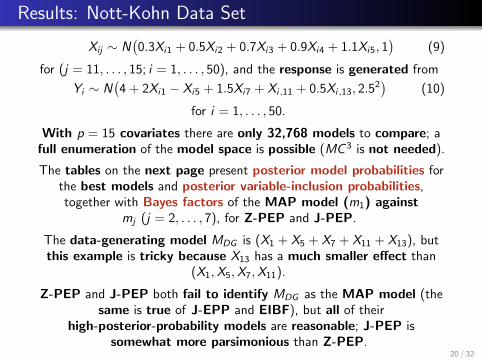
Results: Nott-Kohn Data Set

Xij ∼ N(0.3Xi1 + 0.5Xi2 + 0.7Xi3 + 0.9Xi4 + 1.1Xi5, 1

)(9)

for (j = 11, . . . , 15; i = 1, . . . , 50), and the response is generated from

Yi ∼ N(4 + 2Xi1 − Xi5 + 1.5Xi7 + Xi,11 + 0.5Xi,13, 2.5

2)

(10)

for i = 1, . . . , 50.

With p = 15 covariates there are only 32,768 models to compare; afull enumeration of the model space is possible (MC 3 is not needed).

The tables on the next page present posterior model probabilities forthe best models and posterior variable-inclusion probabilities,together with Bayes factors of the MAP model (m1) against

mj (j = 2, . . . , 7), for Z-PEP and J-PEP.

The data-generating model MDG is (X1 + X5 + X7 + X11 + X13), butthis example is tricky because X13 has a much smaller effect than

(X1,X5,X7,X11).

Z-PEP and J-PEP both fail to identify MDG as the MAP model (thesame is true of J-EPP and EIBF), but all of their

high-posterior-probability models are reasonable; J-PEP issomewhat more parsimonious than Z-PEP.

20 / 32

Results: Nott-Kohn Data Set

Posterior model probabilities for the best models, together withBayes factors of the MAP model (m1) against mj (j = 2, . . . , 7), for theZ-PEP and the J-PEP prior methodologies in the simulated example of

Nott and Kohn.

Z-PEP J-PEPPosterior Model Bayes Posterior Model Bayes

mj Predictors Probability Factor Rank Probability Factor

1 X1 + X5 + X7 + X11 0.0783 1.00 (2) 0.0952 1.002 X1 + X7 + X11 0.0636 1.23 (1) 0.1054 0.903 X1 + X5 + X6 + X7 + X11 0.0595 1.32 (3) 0.0505 1.884 X1 + X6 + X7 + X11 0.0242 3.23 (4) 0.0308 3.095 X1 + X7 + X10 + X11 0.0175 4.46 (5) 0.0227 4.196 X1 + X5 + X7 + X10 + X11 0.0170 4.60 (9) 0.0146 6.537 X1 + X5 + X7 + X11 + X13 0.0163 4.78 (10) 0.0139 6.87

Posterior variable-inclusion probabilities for the Z-PEP and J-PEP priormethodologies for the simulated example of Nott and Kohn.

CovariateMethod X1 X2 X3 X4 X5 X6 X7 X8Z-PEP 0.997 0.110 0.129 0.133 0.503 0.337 1.000 0.150J-PEP 0.993 0.088 0.108 0.121 0.395 0.253 1.000 0.117

CovariateMethod X9 X10 X11 X12 X13 X14 X15Z-PEP 0.126 0.197 0.856 0.136 0.142 0.111 0.113J-PEP 0.100 0.152 0.789 0.109 0.115 0.099 0.100

21 / 32

Sensitivity Analysis for the Training Sample Size n∗

To examine the sensitivity of the PEP approach to the sample sizen∗ of the training data set, we present results for n∗ = 17, . . . , 50.

The figures on the next two pages display posterior marginalvariable-inclusion probabilities and

posterior model probabilities, respectively.

As noted previously, to specify X∗ when n∗ < n we randomlyselected a sub-sample of the rows of the original matrix X.

Results are presented for Z-PEP; J-PEP produced similar findings:

• Both posterior inclusion probabilities andposterior modelprobabilities are quite insensitive to a wide variety of values of n∗.

• Therefore we can use n∗ = n and dispense with training samplesaltogether; this yields the following advantages: increased stability ofthe resulting Bayes factors, removal of the arbitrariness arising from

individual training-sample selections, and substantial increases incomputational speed, allowing many more models to be compared

within a fixed CPU budget.

22 / 32


Posterior marginal inclusion probabilities for different n∗ with the Z-PEPprior methodology for the simulated example of Nott and Kohn.

20 25 30 35 40 45 50

0.0

0.2

0.4

0.6

0.8

1.0

nstar

Pos

terio

r In

clus

ion

Pro

babi

litie

s

X5

X6

X7

X10

X11

X13

X1

23 / 32


Posterior model probabilities of the five best models obtained for each n∗,with the Z-PEP prior methodology for the simulated example of

Nott and Kohn.

20 25 30 35 40 45 50

0.00

0.02

0.04

0.06

0.08

0.10

0.12

0.14

nstar

Pos

terio

r M

odel

Pro

babi

litie

s

X_1+X_5+X_6+X_7+X_11X_1+X_5+X_7+X_10+X_11X_1+X_5+X_7+X_11X_1+X_6+X_7+X_11X_1+X_7X_1+X_7+X_10+X_11X_1+X_7+X_11

24 / 32

Comparisons With IBF and J-EPP

Here we compare the PEP Bayes factor between the two bestmodels ((X1 + X5 + X7 + X11) and (X1 + X7 + X11)) with the

corresponding Bayes factors using J-EPP and IBF.

For IBF and J-EPP we randomly selected 100 training samples ofsize n∗ = 6 (the minimal training sample size for comparison of

these two models) and n∗ = 17 (the minimal training sample size forthe estimation of the full model with all p = 15 covariates), while for

Z-PEP and J-PEP we randomly selected 100 training samples ofsizes n∗ = 6, 17 and n∗ = 5× k for k = 5, . . . , 10.

The figure on the next page presents the results as parallel boxplots,and shows that

• With modest n∗ values, which would tend to be favored by users fortheir advantage in computing speed, the IBF method exhibited an

extraordinary amount of instability across the particular randomtraining samples chosen, and the J-EPP method was

not much better; and

• In contrast, J-PEP and Z-PEP are highly stable as a function oftraining sample.

25 / 32

Comparisons With IBF and J-EPP (continued)

Boxplots of the Intrinsic Bayes Factor (IBF) and Bayes factors using theJ-EPP, J-PEP and Z-PEP approaches, on a logarithmic scale, in favor of

model (X1 + X5 + X7 + X11) over model (X1 + X7 + X11) for thesimulated example of Nott and Kohn.

IBF_6

EPP_J6

PEPP_Z6

PEPP_J6

IBF_17

EPP_J17

PEPP_Z17

PEPP_J17

PEPP_Z30

PEPP_J30

PEPP_Z40

PEPP_J40

PEPP_Z50

PEPP_J50

−4 −2 0 2

Log Bayes Factor

26 / 32

Ozone Application

Full-enumeration search for the full space with 56 covariates wascomputationally infeasible, so we used the model search algorithm

(MC 3) described above for Z-PEP and EIBF.

With such a large number of predictors, the model space in ourproblem is too large for the MC 3 approach to estimate posterior

model probabilities with high accuracy in a reasonable amount ofCPU time.

For this reason, we implemented the following two-step method:

(1) First we used MC 3 to identify variables with high posteriormarginal inclusion probabilities, and we created a reduced model

space consisting only of those variables whose marginal probabilitieswere above a threshold value of 0.3.

(2) Then we used the same model search algorithm as in step (1) inthe reduced space to estimate posterior model probabilities.

The tables on the next two pages show that the PEP methodologysupports more parsimonious models than the EIBF approach.

27 / 32

Ozone Application (continued)

Posterior inclusion probabilities using Z-PEP, J-PEP and EIBF for thereduced model space of the ozone data set.

Index Name J-PEP Z-PEP EIBF1 Day of year 1.000 1.000 1.0002 Wind speed at LAX 0.985 0.992 0.9765 Temperature at Sandburg 0.182 0.375 0.4757 PG from LAX to Daggett 0.613 0.857 0.9848 Inversion base temperature at LAX 1.000 1.000 1.0009 Visibility at LAX 1.000 1.000 1.000

10 (Day of year)2 1.000 1.000 1.000

12 (500 mb pressure height at VAFB)2 0.618 0.840 0.980

13 (Humidity at LAX)2 0.716 0.918 1.000

15 (Inversion base height at LAX)2 0.983 0.988 1.000

16 (PG from LAX to Daggett)2 1.000 1.000 1.000

18 (Visibility at LAX)2 0.896 0.965 0.995

20 (Inversion base temperature at LAX)3 0.401 0.641 0.92323 (Day of year) × (Humidity at LAX) 0.006 0.011 0.02726 (Day of year) × (PG from LAX to Daggett) 0.042 0.093 0.23330 (Wind speed at LAX) × (Humidity at LAX) 0.011 0.027 0.07336 (500 mb pressure height at VAFB) × (Humidity at LAX) 0.036 0.087 0.10039 (500 mb pressure height at VAFB) ×

(PG from LAX to Daggett) 0.040 0.159 0.37142 (Humidity at LAX) × (Temperature at Sandburg) 0.315 0.429 0.69443 (Humidity at LAX) × (Inversion base height at LAX) 0.974 0.898 0.87748 (Temperature at Sandburg) × (PG from LAX to Daggett) 0.017 0.026 0.02851 (Inversion base height at LAX) ×

(PG from LAX to Daggett) 0.065 0.197 0.342

28 / 32


Posterior odds (PO1k) of the five best models within each analysis versusthe current model k, for the reduced model space of the ozone data set.

J-PEPRanking Number of Posterior

J-PEP Z-PEP EIBF Additional Variables Covariates Odds PO1k

1 (>5) (>5) 9 1.002 (1) (5) X7 + X12 + X13 +X20 13 1.293 (>5) (>5) X7 + X13 +X20 12 1.464 (>5) (>5) X12 +X20 11 1.875 (>5) (>5) X12 10 2.08

Z-PEPRanking Number of Posterior

Z-PEP J-PEP EIBF Additional Variables Covariates Odds PO1k

1 (2) (5) X7 + X12 + X13 +X20 13 1.002 (>5) (>5) X5+ X7 + X12 + X13 +X20 14 1.193 (>5) (3) X5+ X7 + X12 + X13 +X20 +X42 15 1.774 (>5) (1) X7 + X12 + X13 +X20 +X42 14 1.945 (>5) (>5) X7 + X12 + X13 12 2.30

EIBFRanking Number of Posterior

EIBF J-PEP Z-PEP Additional Variables Covariates Odds PO1k

1 (>5) (4) X7 + X12 + X13 +X20 +X42 14 1.002 (>5) (>5) X5+ X7 + X12 + X13 +X20+X26 + X42 16 1.173 (>5) (3) X5+ X7 + X12 + X13 +X20 +X42 15 1.304 (>5) (>5) X7 + X12 + X13 +X20+X39 + X42 15 1.445 (2) (1) X7 + X12 + X13 +X20 13 1.58

29 / 32


Comparison of the predictive performance of the PEP and J-EPPmethods, using the full and MAP models in the reduced model space of

the ozone data set.RMSE∗

Model d` R2 R2adj J-PEP Z-PEP J-EPP Jeffreys Prior

Full 22 0.8500 0.8392 0.5988 0.5935 0.6194 0.5972(0.0087) (0.0097) (0.0169) (0.0104)

J-PEP MAP 9 0.8070 0.8016 0.5975 0.6161 0.7524 0.6165(0.0063) (0.0051) (0.0626) (0.0052)

Z-PEP MAP 13 0.8370 0.8303 0.5994 0.5999 0.6982 0.5994(0.0071) (0.0060) (0.0734) (0.0049)

EIBF MAP 14 0.8398 0.8326 0.6182 0.5961 0.6726 0.5958(0.0066) (0.0072) (0.0800) (0.0061)

Comparison with the full model (percentage changes)

RMSE

Model d` R2 R2adj J-PEP Z-PEP J-EPP Jeffreys Prior

J-PEP MAP −59% −5.06% −4.48% −0.22% +3.81% +21.5% +3.23%Z-PEP MAP −41% −1.50% −1.06% +0.10% +1.01% +12.7% +0.37%EIBF MAP −36% −1.20% −0.78% +3.24% +0.44% +10.9% −0.23%

The PEP priors choose more parsimonious models than EIBF and J-EPP,while simultaneously having better out-of-sample predictive accuracy; in

fact they achieve the same predictive accuracy as the independenceJeffreys prior (IJP) applied to the same models (and IJP cannot be used for

variable selection because the Jeffreys prior is improper).30 / 32


Distribution of RMSE across 50 random partitions of the ozone data set,for the Jeffreys-prior, J-EPP, Z-PEP and J-PEP methods, in four

different models.

PEPP_Z

EPP_J

Jeffreys

PEPP_J

0.60 0.65 0.70 0.75 0.80 0.85 0.90

(a) Full Model

PEPP_Z

EPP_J

Jeffreys

PEPP_J

0.60 0.65 0.70 0.75 0.80 0.85 0.90

(b) MAP Model from Power−Expected−Posterior Prior (Zellner’s baseline)

PEPP_Z

EPP_J

Jeffreys

PEPP_J

0.60 0.65 0.70 0.75 0.80 0.85 0.90

(c) MAP Model from Expected−Posterior Prior (Jeffreys baseline)

PEPP_Z

EPP_J

Jeffreys

PEPP_J

0.60 0.65 0.70 0.75 0.80 0.85 0.90

(d) MAP Model from Power−Expected−Posterior Prior (Jeffreys baseline)

31 / 32

Conclusions

The major contribution of the research presented here is to sharplydiminish the effect of training samples on previously-studied

expected-posterior-prior and intrinsic-Bayes-factor methodologies;our method

• is systematically more parsimonious (under either baseline priorchoice) than the EPP approach using the Jeffreys prior as a baseline

prior and minimal training samples, while sacrificing no desirableperformance characteristics to achieve this parsimony;

• is robust to the size of the training sample, thus supporting theuse of the entire data set as a “training sample” and thereby

— promoting stability of the resulting Bayes factors,

—avoiding arbitrariness arising from individual training-sampleselections, and

— achieving fast computation, allowing many more models to beexamined in a fixed CPU budget; and

• identifies maximum a-posteriori models that achieve goodout-of-sample predictive performance.

32 / 32

power-expected-posterior priors for variable selection in ...draper/draper-isba-2012-talk.pdf ·...

Documents