power differential based wide area protectionijeee.iust.ac.ir/article-1-56-en.pdfpower differential...

Iranian Journal of Electrical & Electronic Engineering, Vol. 1, No. 3, July 2005 53

Power Differential based Wide Area Protection F. Namdari, S. Jamali and P. A. Crossley

Abstract: Current differential based wide area protection (WAP) has recently been proposed as a technique to increase the reliability of protection systems. It increases system stability and can prevent large contingencies such as cascading outages and blackouts. This paper describes how power differential protection (PDP) can be used within a WAP and shows that the algorithm operates correctly for all types of system faults whilst preventing unwanted tripping, even if the data has been distorted by CT saturation or by data mismatches caused by delays in the WAP data collection system. The PDP algorithm has been simulated and tested on an Iranian 400kV transmission line during different fault and system operating conditions. The proposed operating logic and the PDP algorithm were also evaluated using simulation studies based on the Northern Ireland Electricity (NIE) 275 kV network. The results presented illustrate the validity of the proposed protection. Keywords: Wide area protection, Power differential algorithm, Current differential relaying, Transmission networks.

1 Introduction1 Busbars and transmission lines are of crucial importance in transferring electrical energy from bulk generating plants to distribution networks. This importance is recognized by the reliability of the protection systems and their ability to remain stable under all possible non-fault operating conditions, whilst operating correctly during a short-circuit fault [1-2]. One of the best methods to achieve the required balance between stability and dependability is wide area protection [3-12]. In a WAP the data collected from all the lines ends and busbars are transferred to a main control center and the performance of the overall system monitored. Under fault conditions, or when the power system is close to instability, the WAP will trip an appropriate selection of circuit breakers. The simplest WAP function is differential protection based on the comparison of the current signals at the line ends. If the input current to a circuit element differs significantly from the output current, a fault condition is detected and

Iranian Journal of Electrical & Electronic Engineering, 2005. Paper first received 6th March 2006 and in revised from 15th July 2006. F. Namdari is a PhD Student at the Department of Electrical Engineering, Iran University of Science & Technology, Tehran, Iran. S. Jamali is with the same Department. P. A. Crossley is with the School of Electrical and Electronic Engineering, Queen's University Belfast, BT9 5AH, Belfast, UK. E-mail: [email protected], [email protected], [email protected].

the element is isolated, by tripping its circuit breakers [9-11]. Adequate protection is more difficult when CT saturation and/or data mismatch, distorts some of the collected data and invalidates current comparison. WAP scheme must be adequately robust to cope with such problems. With bad data, fault conditions can be detected using differential algorithms based on mathematically complex techniques; such as symmetrical component vectors operating within a bias current differential protection (CDP) based WAP [12]. Power differential protection has been proposed as a technique that satisfies the need for immunity against bad data, whilst maintaining the advantages of operating simplicity [13]. A new type of WAP based on PDP is proposed in the paper. The wide area based logic is used in combination with conventional bias differential protection schemes. The logic will automatically widen its protection zones when data is distorted or communication delays cause a mismatch. The proposed PDP based WAP was tested on a simulation model of the Northern Ireland Electricity (NIE) network and the results compared with more conventional CDP methods. 2 Differential Protection based Wide Area Protection

2.1 Wide Area Protection As electrical networks become larger and the numbers of interconnections increase, conventional protection

Dow

nloa

ded

from

ijee

e.iu

st.a

c.ir

at 1

8:54

IRD

T o

n M

onda

y Ju

ly 2

nd 2

018

http://ijeee.iust.ac.ir/article-1-56-en.html


systems might not be able to satisfy the needs for system reliability and selectivity of supply. The solution is more advanced protection and control functions based on advanced digital hardware and software, data communications and enhanced information technology. Wide area protection is one of the techniques that can solve classical problems associated with conventional relaying [3-11]. For example, relays normally operate using information from a small part of the system and in many cases from a single monitoring point. However, during an event such as a power swing or cascading outage they need to monitor other parts of the system and the lack of ‘wide area’ information might cause a maloperation. Communication systems can now transfer data, within a time period acceptable for protection, using either micro-wave or fiber optic high speed networks. These can be used to send control signals acquired from monitoring points distributed over the whole system. The main improvement over conventional data communication methods is the use of GPS synchronization to eliminate the effect of data communication delays. After collecting and synchronizing all the data that is required from the electrical network, the effect of bad data must be cancelled. Bad data is caused by CT saturation and data loss in the communication system. Then, based on the synchronized data acquired from the entire system, the protection algorithms are applied. These algorithms must first isolate the faulted region and then by enhancing the transient stability of the system prevent unwanted events such as cascading outages and large blackouts. This is achieved by special control actions such as load shedding or islanding caused by a lack of energy or generator tripping caused by a surplus. Fig. 1 shows a schematic diagram that represents the WAP. Fig. 1 Schematic diagram of a WAP

2.2 Differential Protection based WAP The primary objective of a WAP is to identify and isolate the faulted section using techniques based on differential protection. The new structure of the network is studied; and if it is needed, the WAP will apply extra switching to improve the stability of the network. Two of the main problems are data distortion and data mismatch, but previous publications have not suggested adequate solutions. CT saturation is a cause of data distortion, but new techniques for differential protection such as the use of symmetrical components may resolve the problem. However, such solutions increase the processing time and more advanced hardware maybe required. Therefore wide area protection techniques, based on conventional differential protection, are required. The basic concept described in this paper is based on conventional differential protection, but a tool for solving the problems of bad data, is also proposed

2.2.1 Current Differential Protection Current differential protection (CDP) is widely used to protect transformers, generators, busbars and transmission lines [1-2]. The protection operates by comparing the currents measured at each end of the protected component using Kirchoff’s current law. If a fault occurs inside the protected zone, the vectorial summation of the end currents will be a non-zero signal (Fig. 2), whose magnitude is then compared against an operating threshold dependent on the scalar summation of the same end currents. The protection operates if the former “differential” signal exceeds the latter “bias” setting (Fig. 3). Most CDP algorithms operate on a per phase basis; hence three sets of calculations are required for a 3 phase network. Fig. 2 Schematic Diagram: Current Differential Protection Fig. 3 Bias Characteristic for CDP

L Time Transfer System (e. g. GPS)

Telecommunication System

Central Equipments for Wide Area Protection

x x

TE TE

TE TE

x x

x x

TE TE

TE TE

x x

Time Signals

Trip Signals

Electrical Data

TE : Terminal Equipment

Ct 1

Element

Ct 2

Relay

1I 2I 21 II −

Internal Faults

External Faults

( ) 221 II +

|I1 –

I2|

Dow

nloa

ded

from

ijee

e.iu

st.a

c.ir

at 1

8:54

IRD

T o

n M

onda

y Ju

ly 2

nd 2

018



2.2.2 Power Differential Protection (PDP) A new type of line differential protection that operates using the “Energy Conservation Law” (ECL):- i.e. “energy in a system may neither be created nor destroyed, just converted from one form into another”[13] is described in the paper. This law when expressed in protection terms, states that the summation of the energy input to the line during a non-fault condition is equal to the output energy. However, when a fault occurs, some of the energy is converted into heat or light and the balance is destroyed. To simplify the proposal, the forward relationship between energy and power, i.e. Energy = Power x time, allows the input and output active power of the line to be used by the relay. If the difference between the real power signals, measured at the ends of the line, is greater than a pre-specified threshold, the relay detects an internal fault and activates the tripping of the circuit breakers. Fig. 4 shows a schematic diagram that describes the power differential protection. To cope with line losses the new protection requires a modified bias characteristic, as shown in Fig. 5 and discussed later in the paper. Fig. 4 Schematic of PDP for a double-ended element Fig. 5 Bias characteristic for PDP algorithm To eliminate the effect of data mismatch and CT saturation, data from each line end is compared with the data from all the other branches connected to the busbar section where the original line was connected. If they do not agree, with respect to Kirchoff’s current law, data mismatch or CT saturation must have occurred in one of the lines ends. This must be recognized and corrected using data acquired from the other lines. If this is necessary, the protection zone must be made larger to cope with the region it now covers. This function is similar to the current differential technique proposed in [11] for the wide area protection of busbars. The main advantages of the new algorithm (PDP) over more

conventional current differential protection schemes (CDP) are: a) Reduction in Data Transfer requirements: - A wide area CDP requires three complex phase current vectors from each of the monitoring points, i.e. at each line end six data packages are needed. - PDP only requires one data package from each line end (real power instantaneous value). Therefore the communication bandwidth for PDP is 1/6 of CDP. b) Reduction in calculation time: - If CDP is applied to a double-ended element, the input phasors from both ends must be converted to real and imaginary components: this involves one sine, one multiply, two squares, one summation and one square root operations; they must then be subtracted (two summation operations for the real part and two for the imaginary part). Finally the result must be converted into a phasor for use as the input to the bias characteristic (two squares, one summation, and one square root operations). - For PDP on a double-ended element, only two values need to be subtracted. - The summation of the signals received from both ends (horizontal vectors of bias characteristics) needs the same calculations for both methods. Therefore the calculations required with PDP are significantly decreased as compared to CDP. Test results obtained using a simple MATLAB program with inputs of the same size, and " 10E9 " iterations shows that the calculations is decreased > 2000 times. c) Application to long lines or cables - CDP has problems on long lines or cables because of the high value of charging current. - PDP is suitable for long lines because it is based on real power and therefore a new operating characteristic is used, see the result’s section. The main disadvantage of PDP is that it cannot recognize the faulted phase, therefore if single pole tripping is required, it cannot be used for primary protection and its use is limited to backup protection. This problem is resolved by using a separate phase selector in the protection scheme. A schematic diagram showing the output of the bias differential characteristics used in the PDP is shown in Fig. 6. Fig. 6 Bias characteristics output schematic of PDP initial trip signals

Element

Relay With Special Characteristic

Real Power 1

( )1P

Real Power 2

( )2P

Internal Faults External

Faults

( ) 221 PP +

|P1 –

P2|

ABS

ABS

ABS

+ +

+ -

P1

P2 Y axis

X axis

TRIP = 1

TRIP = 0

TRIP

Dow

nloa

ded

from

ijee

e.iu

st.a

c.ir

at 1

8:54

IRD

T o

n M

onda

y Ju

ly 2

nd 2

018



The PDP used for busbar protection is the same as the one used for line protection, but in this case the protection zone must have more than two ends. The initial TRIP signals obtained for the studied network are combined using the new logic derived separately for each line and busbar. 3 Proposed Logic for PDP Based WAP As discussed previously, output for the conventional bias characteristics of the differential protection that is named Bias Differential Characteristics (BDP) cannot detect faults under conditions of distorted and mismatched data. In this section a new logic is proposed that uses the outputs of conventional high speed protection techniques. The main ideas for the simple system shown in Fig. 7-a are:

T_1 = [ (a1b) & (cd1b) & (~ c2g) & (~ d3h) ] or [ (a1b) & (a1ef) & ( ~ e4i ) & ( ~ f5j ) ] (1)

T_A = ( acd ) & [ ( cd1b ) or ( cd1ef ) ]& [ (ad2g ) or ( ad2kl ) ] & [ ( ac3h ) or ( ac3mn ) ] (2)

where: a1b: Internal TRIP signal from BDP for line1, using collected data on a and b. cd1b: Internal TRIP signal from BDP for line1, using collected data on b, c and d. a1ef: Internal TRIP signal from BDP for line1, using collected data on a, e and f. acd: Internal TRIP signal from BDP for busbar A, using collected data on a, c and d. T_1: Final TRIP signal for line 1. And T_A: Final TRIP signal for busbar A. Initial TRIP signals can be produced with CDP or PDP algorithms. At first, calculations for producing final TRIP signals seem high, but initial TRIP signals for various lines and busbar are common Basic concept of the proposed algorithm is to extend protection zone in case of data mismatch. Let's assume, data from transmitter a is distorted or mismatched. In this case, based on protection concepts [11], zone of protection automatically will be widened and protection zone for T_A will cover line 1 and the zone of protection will be cdb. The logic will be extended for adding the line 10 to the busbar A ( fig 7-b) as:

T_1 = [ (a1b) & (cds1b) & (~ c2g) & (~ d3h) & (~ s10t) ] or [ ( a1b) & (a1ef) & ( ~ e4i ) & ( ~ f5j )]

(3)

T_A = (acds) & [ (cds1b) or (cds1ef ) ] & [ (ads2g) or (ads2kl) ] & [ (acs3h) or (acs3mn) ] & [ (acd10t) or (acd10u) ]

(4)

Also extending the logic for fig 7-c to show it on a H-arrangement of breakers, is as:

T_1 = [ (a1b) & (cw1b) & (~ c2g) & (~ wds) ] or [ ( a1b) & (a1ef) & ( ~ e4i ) & ( ~ f5j ) ] (5)

T_A = (acw ) & [ (cw1b ) or (cw1ef ) ] & [ (aw2g ) or (aw2kl ) ] & [ (acds ) ]

(6)

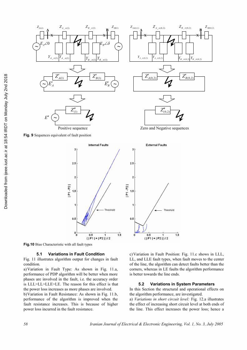
Basic assumptions for the proposed logic are: - Only one transmitter per each busbar sends mismatched or distorted data (for CDP based WAP, one transmitter per phase per busbar). - If busbar protection operates, all of the connected lines to the busbar must be disconnected. Both of the concepts are acceptable in power transmission system studies, because usually when CT saturation or data mismatch as a result of the high current in a CT occurred, the high current will be distributed between the other CT's connected to the busbar. Also for the second concept, if busbar protection operates, all of the lines connected to the busbar will not carry any energy and they must be disconnected. 4 PDP Algorithm Formulation The equations required to implement the PDP algorithm are obtained in this Section. A simple faulted transmission line diagram is shown in Fig. 8, where L is the total line length and p is the per unit fault position. The networks beyond the two end busbars are represented by their equivalent Thevenin networks, as is a normal practice in the protection studies. For a more realistic simulation under all fault types and operational conditions, a distributed π line model has been used [15]. The circuit positive, negative and zero sequence networks and their Thevenin equivalent circuits, from the fault point of view, are shown in Fig. 9. In these diagrams and the following equations, subscripts 0, 1 and 2 stand for zero, positive and negative sequence values, respectively. Based on the system reduction shown in Fig. 9, the following equations have been used to derive the voltage and the impedance of the equivalent Thevenin for the sequence networks:

( )l.p.sinhZZ c_A γ=π (7)

γ= −

π 2l.p.tanh.ZY 1

c_A (8)

( )

+++

=′

−π

−π

π−

π−

π

−π

ASA

1_A

1_A

_A1

_ASA1

_A

1_A

A

E.ZY

Y.

ZY||ZY

Y

E

(9)

( )( ) 1_A_A

1_ASAA Y||ZY||ZZ −

ππ−

π +=′ (10)

BA Z||ZZ ′′=′′ (11)

Z.ZE

ZE

EB

B

A

A ′′

′′

+′′

=′′ (12)

Equations for determining fault currents and voltages have been presented in Appendix A.

Dow

nloa

ded

from

ijee

e.iu

st.a

c.ir

at 1

8:54

IRD

T o

n M

onda

y Ju

ly 2

nd 2

018



Fig. 7 Simple electrical grids The sequence voltages and currents at the relaying point “A” are as follows:

( ))1(_A

1

)1(_A)1(SA

)1(faultA

)1(SA1

)1(_A

1

)1(_A

)1(A ZY||Z

vE.ZY

Y

iπ

−π

−π

−π

+

−

+=

(13)

)1(_A)1(A)1(fault)1(A Z.ivv π+= (14)

( ))2,0(_A

1

)2,0(_A)2,0(SA

)2,0(fault)2,0(A ZY||Z

vi

π−

π +−= (15)

)2,0(_A)2,0(A)2,0(fault)2,0(A Z.ivv π+= (16)

From the above voltages and currents the real power is obtained:

( ))0(A)0(A)2(A)2(A)1(A)1(AA i.vi.vi.vreal.3P ++= (17)

If all “A” subscripts in the above equations are replaced with “B” and “p” is replaced with “1-p”, then the equations are also valid for the relaying point at busbar “B” of the simulated line. 5 PDP Simulation Studies The validity of the proposed algorithm has been tested using simulation studies based on typical Iranian 400 kV line data. The line series and shunt parameters are given in [14] where the line shunt capacitance has been calculated by using the line conductors’ geometry. For the circuit shown in Fig. 8, the relevant line parameters and circuit data are given in Appendix B.

The algorithm has been tested for different fault positions along the line for all fault types, including single-phase-to-earth (LE), double-phase-to-earth (LLE), double-phase (LL), and three-phase (LLL) faults. In this part of the paper, outputs of PDP algorithm for all fault types in different positions on the line are studied. Fault resistance has also been considered in the study, where for LE, LLE and LLL faults the fault resistance varies from 0 to 100 ohms and for LL faults this varies from 0 to 20 ohms, in certain steps. All internal and external faults have been modelled using MATLAB Symbolic Toolbox, which discards effects of discrete calculations associated with digital measurement and protection. Position of cases studied on PDP bias characteristic is shown in Fig. 10. The PDP algorithm can recognise all internal faults from external ones for the studied system. Effects of variations in system and fault parameters have been studied in two categories of fault conditions and system operational conditions before the fault. Fig. 8 Schematic for simulated system

I

o k

G

H

J

C

D

A

B

E

F

p

q

r

l

m

n

g c

h d

a b e i

f j 1

2

3

6

7

8

9

4

5

A ... J : Busbars a ... r : Circuit Breakers 1 ... 9 : Transmission Lines

x

x

x

x

x

x

x x

x

x

x

x

x

x

x

x x

x

(a)

I

o k

G

H

J

C

D

A

B

E

F

p

q

r

l

m

n

g c

h d

a b e i

f j 1

2

3

6

7

8

9

4

5

A ... L : Busbars a ...v : Circuit Breakers 1 ...11 : Transmission Lines

x

x

x

x

x

x

x x

x

x

x

x

x

x

x

x x

x s t

10 x x K

(b)

u v 11 x x

L

I

o k

G

H

J

C

D

A

B

E

F

p

q

r

l

m

n

g c

h d

a b e i

f j 1

2

3

6

7

8

9

4

5

A ... M : Busbars a ..w : Circuit Breakers 1 ...11 : Transmission Lines

x

x

x

x

x

x

x x

x

x

x

x

x

x

x

x x

x s t

10 x x K

xw

(c)

u v 11 x x

L M

Transmission Line

Fault

SBZ

0∠AE δ∠BE p.L (1-p).L

SAZ B A

x x

~ ~

Dow

nloa

ded

from

ijee

e.iu

st.a

c.ir

at 1

8:54

IRD

T o

n M

onda

y Ju

ly 2

nd 2

018



Fig. 9 Sequences equivalent of fault position

Fig.10 Bias Characteristic with all fault types

5.1 Variations in Fault Condition Fig. 11 illustrates algorithm output for changes in fault condition. a) Variation in Fault Type: As shown in Fig. 11.a, performance of PDP algorithm will be better when more phases are involved in the fault, i.e. the accuracy order is LLL>LL>LLE>LE. The reason for this effect is that the power loss increases as more phases are involved. b) Variation in Fault Resistance: As shown in Fig. 11.b, performance of the algorithm is improved when the fault resistance increases. This is because of higher power loss incurred in the fault resistance.

c) Variation in Fault Position: Fig. 11.c shows in LLL, LL, and LLE fault types, when fault moves to the center of the line, the algorithm can detect faults better than the corners, whereas in LE faults the algorithm performance is better towards the line ends.

5.2 Variations in System Parameters In this Section the structural and operational effects on the algorithm performance, are investigated. a) Variations in short circuit level: Fig. 12.a illustrates the effect of increasing short circuit level at both ends of the line. This effect increases the power loss; hence a

0∠AE δ∠BE

)1(SAZ )1(SBZ

)1(_πBZ )1(_ πAZ

)1(_πBY )1(_ πAY

)1(BZ ′ )1(AZ ′

AE′

)1(Z ′′ E ′′

BE′

)1(_ πAY )1(_πBY

A Bx x

~ ~

~ ~

~

)2,0(BZ ′ )2,0(AZ ′

)2,0(Z ′′

)2,0(SAZ )2,0(SBZ

)2,0(_ πBZ )2,0(_πAZ

)2,0(_πBY )2,0(_πBY )2,0(_πAY

)2,0(_πAY

x xA B

Positive sequence Zero and Negative sequences

Dow

nloa

ded

from

ijee

e.iu

st.a

c.ir

at 1

8:54

IRD

T o

n M

onda

y Ju

ly 2

nd 2

018



better performance by the algorithm. In this case the threshold level must be increased in y-axis direction. b) Variation in voltage ratio: As shown in Fig. 12.b, when voltage increases at the line ends with higher load angle, in-zone fault position in bias characteristic goes further away from both x and y axes. c) Variation in load angle: Fig. 12.c shows that the increase in load angle results in better performance of the algorithm. d) Variation of line length: As shown in Fig. 12.d, for LLL internal faults, fault position in the bias characteristic will be further away from the threshold level, but fault positions for LE, LL, and LLE internal faults will be closer to the threshold level; elsewhere, with the increased line length, external fault positions come down in y-axis direction. Therefore, the threshold level for longer lines must be closer to x-axis. e) Effects of shunt and series line parameters: Extra studies show variations in line series resistance and shunt capacitance do not affect the algorithm accuracy; but when line series inductance increases, the threshold level must be closer to x-axis. Summary of figs. 11-12 has been illustrated in table 1.

6 Case Study for PDP based WAP The proposed PDP based WAP method has been developed for Northern Ireland Electricity (NIE) 275 kV simulated network using PSCAD/EMTDC. The single line diagram of the NIE network is shown in Fig.13. The simplified network diagram contains 9 busbars, 17 transmission lines, 3 lumped generators, 6 lumped loads, and a capacitor bank. The HVDC link to Scotland has been considered as a generator. Electrical parameters of the network have been presented in Appendix C. In this network single line tripping is not applied, therefore in our simulations, power differential protection (PDP) has been used as main function for producing initial TRIP signals of wide area protection logic. In cases where protection philosophy of the system is based on single line tripping, PDP based WAP can be used as backup of conventional protection system [13]. It is assumed, all the required data are being synchronized using GPS before transmitting to the WAP control centre.

Fig. 11 Effects of different fault conditions on the PDP algorithm

b) Variation of Fault Resistance

c)Variation of Fault Position

0 0.2 0.4 0.6 0.8 1 1.2 1.40

0.5

1

1.5

2

2.5

( | P1 | + | P2 | )/2 in PU

| P1

- P2

| in

PU

Fault Resistance=8 Ω for Internal and External Faults(Fault Position for Internal Faults = 0.2 of Line Length)

Three Phase FaultSingle Phase to Earth FaultDouble Phase FaultDouble Phase to Earth FaultExternal Faults

0 0.2 0.4 0.6 0.8 1 1.2 1.40

0.5

1

1.5

2

2.5

( | P1 | + | P2 | )/2 in PU

| P1

- P2

| in

PU

Variable Fault Resistances for Internal and External Faults(Fault Position for Internal Faults = 0.2 of Line Length)

LLL Fault ( Rf = 1 Ω)LLL Fault ( Rf = 8 Ω)LLL Fault ( Rf = 12 Ω)LE Fault ( Rf = 1 Ω)LE Fault ( Rf = 8 Ω)LE Fault ( Rf = 12 Ω)LL Fault ( Rf = 1 Ω)LL Fault ( Rf = 8 Ω)LL Fault ( Rf = 12 Ω)LLE Fault ( Rf = 1 Ω)LLE Fault ( Rf = 8 Ω)LLE Fault ( Rf = 12 Ω)External Faults

0 0.2 0.4 0.6 0.8 1 1.2 1.40

0.5

1

1.5

2

2.5

3

( | P1 | + | P2 | )/2 in PU

| P1

- P2

| in

PU

Variable Fault Position for Internal Faults(Fault Resistance = 8 Ω )

LLL Fault (Pos.=0.1 of Line Length)LLL Fault (Pos.=0.3 of Line Length)LLL Fault (Pos.=0.5 of Line Length)LE Fault (Pos.=0.1 of Line Length)LE Fault (Pos.=0.3 of Line Length)LE Fault (Pos.=0.5 of Line Length)LL Fault (Pos.=0.1 of Line Length)LL Fault (Pos.=0.3 of Line Length)LL Fault (Pos.=0.5 of Line Length)LLE Fault (Pos.=0.1 of Line Length)LLE Fault (Pos.=0.3 of Line Length)LLE Fault (Pos.=0.5 of Line Length)

a)Variation of Fault Type

Dow

nloa

ded

from

ijee

e.iu

st.a

c.ir

at 1

8:54

IRD

T o

n M

onda

y Ju

ly 2

nd 2

018



Fig 12 Effects of variation in system parameters on the PDP algorithm Fig. 13 NIE 275 kV network

0 0.2 0.4 0.6 0.8 1 1.2 1.40

0.5

1

1.5

2

2.5

3

( | P1 | + | P2 | )/2 in PU

| P1

- P2

| in

PU

Variable Short Circuit Power for Internal and External Faults( Fault Resistance=8Ω , Fault Position for Internal Faults = 0.2 of Line Length)

LLL Fault ( 20--5 GVA )LLL Fault ( 20--10 GVA )LLL Fault ( 30--30 GVA )LE Fault ( 20--5 GVA )LE Fault ( 20--10 GVA )LE Fault ( 30--30 GVA )LL Fault ( 20--5 GVA )LL Fault ( 20--10 GVA )LL Fault ( 30--30 GVA )LLE Fault ( 20--5 GVA )LLE Fault ( 20--10 GVA )LLE Fault ( 30--30 GVA )External Faults

a) Variation of short circuit power 0 0.2 0.4 0.6 0.8 1 1.2 1.4

0

0.5

1

1.5

2

2.5

( | P1 | + | P2 | )/2 in PU

| P1

- P2

| in

PU

Variable Source Voltage Ratios for Internal and External Faults( Fault Resistance=8Ω , Fault Position for Internal Faults = 0.2 of Line Length)

LLL Fault ( E2/E1=0.9 )LLL Fault ( E2/E1=1.0 )LLL Fault ( E2/E1=1.1 )LE Fault ( E2/E1=0.9 )LE Fault ( E2/E1=1.0 )LE Fault ( E2/E1=1.1 )LL Fault ( E2/E1=0.9 )LL Fault ( E2/E1=1.0 )LL Fault ( E2/E1=1.1 )LLE Fault ( E2/E1=0.9 )LLE Fault ( E2/E1=1.0 )LLE Fault ( E2/E1=1.1 )External Faults

b) Variation of voltage ratio

0 0.2 0.4 0.6 0.8 1 1.2 1.40

0.5

1

1.5

2

2.5

( | P1 | + | P2 | )/2 in PU

| P1

- P2

| in

PU

Variable Load Angles for Internal and External Faults( Fault Resistance=8Ω , Fault Position for Internal Faults = 0.2 of Line Length)

LLL Fault ( δ = 10° )LLL Fault ( δ = 20° )LLL Fault ( δ = 30° )LE Fault ( δ = 10° )LE Fault ( δ = 20° )LE Fault ( δ = 30° )LL Fault ( δ = 10° )LL Fault ( δ = 20° )LL Fault ( δ = 30° )LLE Fault ( δ = 10° )LLE Fault ( δ = 20° )LLE Fault ( δ = 30° )External Faults

c) Variation of load angle 0 0.2 0.4 0.6 0.8 1 1.2 1.4

0

0.5

1

1.5

2

2.5

3

( | P1 | + | P2 | )/2 in PU

| P1

- P2

| in

PU

Variable Line Lengths for Internal and External Faults( Fault Resistance=8Ω , Fault Position for Internal Faults = 0.2 of Line Length)

LLL Fault ( L = 200 Km )LLL Fault ( L = 300 Km )LLL Fault ( L = 400 Km )LE Fault ( L = 200 Km )LE Fault ( L = 300 Km )LE Fault ( L = 400 Km )LL Fault ( L = 200 Km )LL Fault ( L = 300 Km )LL Fault ( L = 400 Km )LLE Fault ( L = 200 Km )LLE Fault ( L = 300 Km )LLE Fault ( L = 400 Km )External Faults

d) Variation of Line Length

~

~

~ G3

G2

G1 Ld6

Ld1

Ld4 Ld3

Ld2

Ld5

C1

L1 L2 L12

L11

L17

L15 L16 L18 L19

L9 L10

L3 L13

L14 L4 L5

A

B

C

D

E

F

G

H

I x

x

x x

x x

1

2 3 4

5 6

Dow

nloa

ded

from

ijee

e.iu

st.a

c.ir

at 1

8:54

IRD

T o

n M

onda

y Ju

ly 2

nd 2

018



Fig. 14 Components of bias characteristic for 3 phase fault caused in line L16 at time .57 second, (a): When data on 2 is lost and data will be collected from 1-3-4-5-6; (b): When data will be collected from 1-2. Fig. 15 Components of bias characteristic for 3 phase fault caused in line L16 at time .57 second, (a): When data on 1 is lost and data will be collected from 1-2; (b): When data on 1 is lost and data will be collected from 1-2.

(|P

1|+|P

2|)/2

(|P1|+

|P2|)

/2

| P1-

P 2|

| P1-

P 2|

Time (Second) Time (Second)

(a) (b)

Time (Second)

(a) Time (Second)

(b)

(|P1|+

|P2|)

/2

| P1-

P 2|

(|P1|+

|P2|)

/2

| P1-

P 2|

Dow

nloa

ded

from

ijee

e.iu

st.a

c.ir

at 1

8:54

IRD

T o

n M

onda

y Ju

ly 2

nd 2

018



Table 1 Summary of PDP simulation studies Ranking of the best

Selectivity Fault Type

Studied Variation Variable Variation Internal

Fault Position (P)

Fault Resistance

Ω LE LL LLE LLL LE 0.2 8 4 - - - LL 0.2 8 - 2 - -

LLE 0.2 8 - - 3 Fault Type Faulted Phase

LLL 0.2 8 - - - 1 1 0.2 - 3 3 3 3 8 0.2 - 2 2 2 2 Fault Resistance Ω

12 0.2 - 1 1 1 1 0.1 - 8 1 3 3 3 0.3 - 8 2 2 2 2 Position of Fault p 0.5 - 8 3 1 1 1

20 – 5 0.2 8 3 1 3 3 20 - 10 0.2 8 2 2 2 2 Short Circuit

Power A-B

(GVA) 30 – 30 0.2 8 1 3 1 1 0.9 0.2 8 3 3 3 3 1.0 0.2 8 2 2 2 2 Voltage Ratio

AB

EE

1.1 0.2 8 1 1 1 1 10 0.2 8 3 3 3 3 20 0.2 8 2 2 2 2 Load Angle °δ 30 0.2 8 1 1 1 1

200 0.2 8 1 1 1 3 300 0.2 8 2 2 2 2 Line Length Km 400 0.2 8 3 3 3 1 0.2 0.2 8 3 3 3 1 1 0.2 8 2 2 2 2 Line Resistance R 5 0.2 8 1 1 1 3

0.833 0.2 8 1 1 1 1 1 0.2 8 2 2 2 2 Line Inductance L

1.2 0.2 8 3 3 3 3 0.5 0.2 8 1 1 1 3 1 0.2 8 1 1 1 2 Line

Capacitance C 2 0.2 8 1 1 1 1

Table 2 Trip format in case of data mismatch or bad data

Position of Fault Non-Mismatched data Mismatched or distorted data

Tripped Elements Position of bad data

Zone containing fault

Tripped Elements

L14 L14 A-L14 A A, L4, L14, L15, L16

L14 L14 D-L14 D D, L5, L14, L18, L19

D D, L5, L14, L18, L19 D-L14 D D, L5, L14, L18, L19

For each line, all types of fault (LE, LLE, LL, and LLL), with fault resistances of 0.1, 1, 10, and 100 ohms have been applied at the 0-ε , 0+ε , 0.25, 0.5 0.75, 1-ε , and 1+ε of the line length with mismatched or distorted data. The distortion factor, i.e. the ratio of measured data to real data, is varied from 0% to 100% in steps of 20% for each end. The above fault types and fault resistance have been applied without and with mismatched and distorted data with the above variation of distortion factor. For all

lines and busbars, under all fault conditions and different distortion factors, the test results show that the PDP based WAP can successfully isolate the faulted section in all cases. To show the effect of the loss of data; figs 14-15 show the bias characteristic for LLL fault caused in line L16 (Fault Resistance = 10 ohms) in normal cases (fig. 14-b), when the data from 1 end is lost and PDP works based on the received data from other branches of the branch with the lost data (fig. 14-a), and when the data

Dow

nloa

ded

from

ijee

e.iu

st.a

c.ir

at 1

8:54

IRD

T o

n M

onda

y Ju

ly 2

nd 2

018



from 1 end is lost and the PDP has not extended the zone of protection (fig 15). These figs show; when the data from one end is lost, extending the zone (Base of the logic) will improve the effect of the PDP algorithm. The processing time for the simulated network and implementing the algorithm is about 20 seconds for the present 2.8 GHz PC, using PSCAD/EMTDC. It means the algorithm can be easily applied as real time in a double paralleled PC, when the network simulation time is reduced and the source codes of the program is used. 7 Conclusions A new power differential protection (PDP) has been proposed as a very fast and effective algorithm for wide area protection (WAP). New logic for wide area protection was also suggested since this eliminates the effects of data mismatch and distortion. Performance of PDP was evaluated for variations in system electrical parameters and fault conditions. From the fault conditions point of view:- increasing the phases involved in fault (from LE to LLL), increasing the fault resistance, and moving the fault closer to the centre of the line for LL, LLE, and LLL faults and closer to the line ends for LE faults, improves the performance of the algorithm. From the system parameters point of view: - an increase in the short circuit levels, an increase in the voltage ratio of the line ends and an increase in the load angle, improves the performance. Increasing line length and the line inductance requires a change in the bias characteristic, but variations in line resistance and capacitance have no effects. The simulation results show the proposed algorithm can operate correctly under all fault conditions and remain stable in non-fault cases such as mismatched and distorted data. The technique is ideal for a wide area protection. The proposed logic can be used with power differential protection applied to wide area protection of networks that use three-phase only tripping. When used on networks that require single and/or three pole tripping a separate phase selector is required. Acknowledgements The authors wish to thank the Northern Ireland Electricity for their support. The authors also wish to acknowledge the support of the Power and Energy Centre of Electrical and Electronic Engineering School – Queen's University of Belfast and Iran Ministry of Science, Research and Technology. References [1] Power System Protection (4 vols.), IEE, Short Run

Press, England, 1995.

[2] Anderson, P.M., Power System Protection, IEEE Press: Mc Graw-Hill, New York, 1999.

[3] Tan, J.C., Crossley, P.A., Mc Laren, P.G., Gale, P.F., Hall, I., and Farrell, J., Application of a wide area backup protection expert system to prevent cascading outages, IEEE Transactions on Power Delivery, Vol. 17 No. 2 , 2002, pp. 375 -380.

[4] Tan, J.C., Crossley, P.A., Mc Laren, P.G., Hall, I., Farrell, J., and Gale, P., Sequential tripping strategy for a transmission network back-up protection expert system, IEEE Transactions on Power Delivery, Vol. 17, No. 1 , 2002, pp. 68 –74.

[5] Rehtanz, C., and Bertsch, J., A new wide area protection system, Power Tech Proceedings of IEEE Porto, Vol.4, 2001, pp. 6.

[6] Novosel, D., Begovic, M., Taylor, C., Clerfeuillie, J., Rhatt, N., and Karlsson, D., Wide Area Protection and Emergency Control, IEEE Power Engineering Society Winter Meeting, Vol. 2, 1999, pp. 917-918.

[7] Ingelsson, B., Lindstrom, P.-O., Karlsson, D., Runvik, G., and Sjodin, J.-O., Wide-area protection against voltage collapse, IEEE Computer Applications in Power, Vol. 10, No. 4, 1997, pp. 30-35.

[8] Serizawa, Y., Imamura, H., and Kiuchi, M., Performance evaluation of IP-based relay communications for wide-area protection employing external time synchronization, IEEE Power Engineering Society Summer Meeting, Vol.2, 2001, pp. 909 -914.

[9] Serizawa, Y., Imamura, H., Sugaya, N., Hori, M., Takeuchi, A., Inukai, M., Sugiura, H., and Kagami, T., Experimental examination of wide-area current differential backup protection employing broadband communications and time transfer systems, IEEE Power Engineering Society Summer Meeting, Vol. 2, 1999, pp. 1070 -1075.

[10] Serizawa, Y., Myoujin, M., Kitamura, K., Sugaya, N., Hori, M., Takeuchi, A., Shuto, I., and Inukai, M., Wide-area current differential backup protection employing broadband communications and time transfer systems, IEEE Transactions on Power Delivery, Vol. 13, No. 4 , 1998, pp. 1046-1052.

[11] Kangvansaichol, K., and Crossley, P.A., Multi-zone Differential Protection for Transmission Networks, 8th Conference on Developments in Power System Protection, Vol. 2, Amsterdam, 2004, pp. 428-432.

[12] Villamagna, N., and Crossley, P. A., Design and Evaluation of a Current Differential Protection Scheme with Enhanced Sensitivity for High Impedance In-Zone Faults on a heavily Loaded

Dow

nloa

ded

from

ijee

e.iu

st.a

c.ir

at 1

8:54

IRD

T o

n M

onda

y Ju

ly 2

nd 2

018



Line, 8th Conference on Developments in Power System Protection-DPSP, Amsterdam, 2004.

[13] Namdari, F., Jamali, S., and Crossley, P. A., Differential Protection of Transmission Lines using Real Power Signals, International Conference on Advanced Power System Automation and Protection, South Korea, 2004.

[14] Jamali, S., and Shateri, H., Robustness of Distance Relay with Mho Characteristic against Fault Resistance, International Conference on Power System Technology – POWERCON, Singapore, 2004.

[15] Stevenson, W.D., Elements of Power System Analysis, 4th Ed., McGraw-Hill Book Co., New York, 1988.

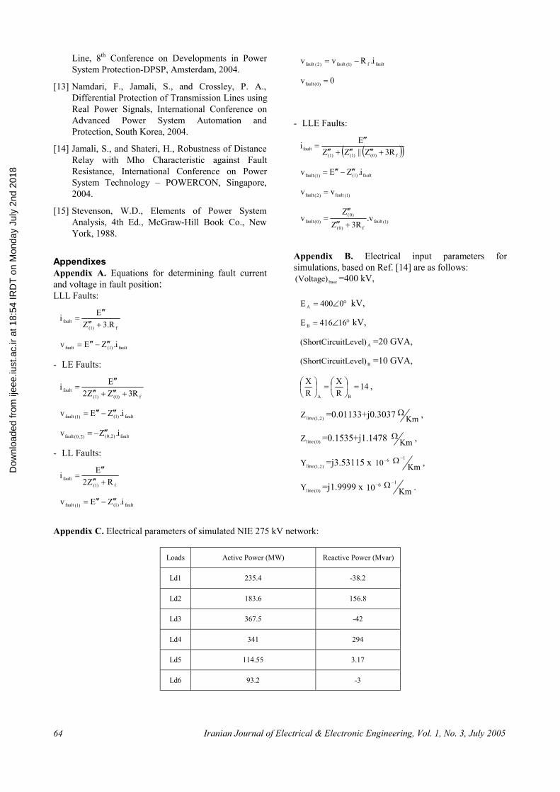
Appendixes Appendix A. Equations for determining fault current and voltage in fault position: LLL Faults:

f)1(fault R.3Z

Ei+′′′

′′′=

fault)1(fault i.ZEv ′′′−′′′=

- LE Faults:

f)0()1(fault R3ZZ2

Ei+′′′+′′′

′′′=

fault)1()1(fault i.ZEv ′′′−′′′=

fault)2,0()2,0(fault i.Zv ′′′−=

- LL Faults:

f)1(fault RZ2

Ei+′′′′′′

=


faultf)1(fault)2(fault i.Rvv −=

0v )0(fault =

- LLE Faults:

( )( )f)0()1()1(fault R3Z||ZZ

Ei+′′′′′′+′′′

′′′=


)1(fault)2(fault vv =

)1(faultf)0(

)0()0(fault v.

R3ZZ

v+′′′

′′′=

Appendix B. Electrical input parameters for simulations, based on Ref. [14] are as follows:

base)Voltage( =400 kV,

°∠= 0400E A kV,

°∠= 16416E B kV,

A)itLevelShortCircu( =20 GVA,

B)itLevelShortCircu( =10 GVA,

14RX

RX

BA

=

=

,

)2,1(lineZ =0.01133+j0.3037 KmΩ ,

)0(lineZ =0.1535+j1.1478 KmΩ ,

)2,1(lineY =j3.53115 x 610−

Km1−Ω ,

)0(lineY =j1.9999 x 610−Km

1−Ω .

Appendix C. Electrical parameters of simulated NIE 275 kV network:

Loads Active Power (MW) Reactive Power (Mvar)

Ld1 235.4 -38.2

Ld2 183.6 156.8

Ld3 367.5 -42

Ld4 341 294

Ld5 114.55 3.17

Ld6 93.2 -3

Dow

nloa

ded

from

ijee

e.iu

st.a

c.ir

at 1

8:54

IRD

T o

n M

onda

y Ju

ly 2

nd 2

018



Generators Active Power (MW) Reactive Power (Mvar)

G1 1255 383.19

G2 368 158.19

G3 451.39 181.685

Capacitor Bank C: Reactive Power (Mvar)

C1 236

Transmission

Lines R[/m] X[/m] B[/m] Length (km)

L_1 6.41883E-08 5.64322E-07 3.39396E-06 37.39

L_10 4.85175E-08 4.25876E-07 2.72776E-06 18.55

L_11 5.06933E-08 4.38348E-07 2.65543E-06 67.07

L_12 5.03282E-08 4.17943E-07 2.70241E-06 45.70

L_13 5.18719E-08 4.42039E-07 2.86423E-06 44.34

L_14 4.85437E-08 4.36893E-07 2.6343E-06 30.90

L_15 5.19031E-08 4.42907E-07 2.6609E-06 28.90

L_16 5.19031E-08 4.42907E-07 2.6609E-06 28.90

L_17 8.04395E-08 6.94526E-07 4.21621E-06 50.97

L_18 5.1353E-08 4.24649E-07 2.75528E-06 50.63

L_19 5.1353E-08 4.24649E-07 2.75528E-06 50.63

L_2 6.41883E-08 5.64322E-07 3.39396E-06 37.39

L_3 5.18719E-08 4.42039E-07 2.86423E-06 44.34

L_4 4.94905E-08 4.36681E-07 2.63173E-06 34.35

L_5 4.90421E-08 4.38314E-07 2.63602E-06 65.25

L_9 4.85175E-08 4.20485E-07 2.72776E-06 18.55

Dow

nloa

ded

from

ijee

e.iu

st.a

c.ir

at 1

8:54

IRD

T o

n M

onda

y Ju

ly 2

nd 2

018


power differential based wide area protectionijeee.iust.ac.ir/article-1-56-en.pdfpower differential...

Documents