power and sample size for time to event - andrew · pdf file11/12/2013 3 the extent of...

11/12/2013

1

Power and Sample size for time

to event analysis

Melania Pintilie

Advanced Statistical Methods for Clinical Trials

Goals

• To understand the 2 types of error in statistics

• To understand the intricacies of sample size

calculation for time to event analysis with and

without competing risks

• To know what information is necessary

• To familiarize with simulations in R

• To know how and what to report

Fall 2013 Advanced Methods in Clinical Trials 2

11/12/2013

2

Type I and II errors

• Significance level (α): The probability of a type I error, that the null hypothesis will be rejected and it will be concluded that there is an effect when in fact there is none. This is usually set to 0.05.

• Power (1-β): where β is the probability of a type II error, the chance of missing a clinically significant difference. Β is usually set as 0.2. Power is usually expressed in percentages like 80%.

• Clinically important difference: The smallest difference in means/proportions/etc that the clinicians feel is worth detecting. This difference can be smaller or larger than observed differences from other trials.


Power vs. sample size

• The same technical approach (the formulae): one is assumed and the other is calculated– Assuming the α level, other parameters (like the effect size)

and the power , the sample size can be calculated– Assuming the α level, other parameters (like the effect size)

and the sample size, the power can be calculated.

• For a randomized clinical trial – sample size

• To test a covariate (like a marker) for which we have the cohort - power

• Sometimes the approach is dictated by what is easier to calculate


11/12/2013

3

The extent of calculation

• A sample size calculation is not usually a single calculation but a set of calculations, which can be presented in a table or graph.

• It is important to be aware of how the required sample size varies according to variations in input parameters, especially those for which the values are more uncertain.


The extent of calculation

• If the sample size is limited by either–Financial constraints

–Available pool of patients or

–Time frame for recruiting

Then calculations should focus on what difference can be detected with the sample size available, and/or the power you have to detect a particular effect of interest.


11/12/2013

4

Working on sample size/power• This is the most ungratifying work for a statistician.

One could spend a week on it but only one sentence would be included in the protocol/grant.

• In spite of this it is an important piece in the design of a study. A wrong calculation could render the study:

– Useless if under-powered. This means that a good treatment will go to waste

– Too long if over-powered. This means that more patients will be given an inefficient treatment.

Fall 2013 Advanced Methods in Clinical Trials

7

Needs to be performed by at least 2 different methods.

1) “By hand” using the formulae

2) Software

3) Simulations

Fall 2013 8

Sample size calculation -survival

1 / 2 1( )

ln( )ev

z zn

HRα β

σ− −+

=

ev

ev

nN

P=

HR = hazard ratio to be detected

σ = standard deviationof the covariate

z1-α/2 = quantile of the standard normal

Advanced Methods in Clinical Trials

Note that the formula for the number of events can be applied regardless

whether the covariate is continuous or categorical.

11/12/2013

5

Understanding the denominator

�� - normalized effect

• �� is in fact the coefficient

• Suppose that age is the covariate of interest

• Say agem=age in month and agey=age in years with

σm=standard deviation for agem and σy =standard deviation

for agey


�� = 12�� = 12�� = ��

12�� = 12��

�� = �� is invariant to the unit of measure

�� is the effect when the covariate is normalized

Calculating the probability of event

(death)


Assuming uniform accrual

a = accrual time, f = follow-up time, λ = the hazard rate for the overall

�� =! � "��#$��"��%&�"�##'(�# "#)

*=

! � "��#$|��%&�"�##'(�# �� %&�"�##'(�# "#)

*=

1 − 1�! - � + � − # "#

)

*= 1 − 1

�! - & "&)/�

�

11/12/2013

6

Calculating the integral


( )

1f f a

ev

e eP

a

λ λ

λ

− − +−= −

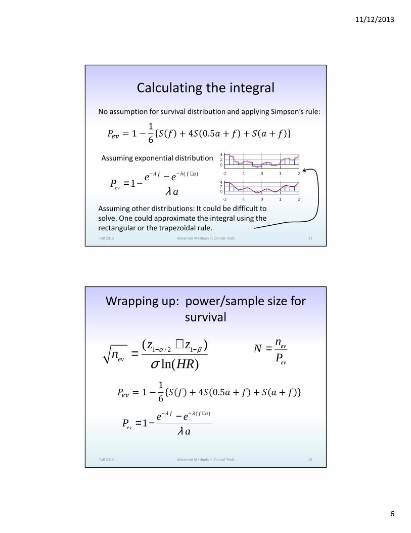
No assumption for survival distribution and applying Simpson’s rule:

�� = 1 − 16 - � + 4- 0.5� + � + - � + �

Assuming exponential distribution

Assuming other distributions: It could be difficult to

solve. One could approximate the integral using the

rectangular or the trapezoidal rule.

Wrapping up: power/sample size for

survival


1 / 2 1( )

ln( )ev

z zn

HRα β

σ− −+

=ev

ev

nN

P=

�� = 1 − 16 - � + 4- 0.5� + � + - � + �

( )

1f f a

ev

e eP

a

λ λ

λ

− − +−= −

11/12/2013

7

Fall 2013 13

A very simple power calculationIf we know or can estimate the number of deaths

in the data set.

A randomized study accrued between 1992-2000. During the study, tumour tissue was collected and kept for future use. Advantages:

•Uniform group of patients•The allocation of treatment is based on randomization not on patient characteristics

Of interest is whether a specific marker (say expression of HIF1α gene) is prognostic for survival.


Fall 2013 14

A very simple power calculation

A genetic signature was developed for a group of patients with lung cancer. The treatment is fairly uniform for this disease.It is desirable to validate the genetic signature.With similar follow-up, the Pev will be similar.

1 / 2 1( )

ln( )ev

z zn

HRα β

σ− −+

= evev

nP

N=

Essential to use the correct Pev, crude rate of the events of interest.


If we know or can estimate the number of deaths

in the data set.

11/12/2013

8

Example 1• 289 patients diagnosed with early stage (1/2)

lung cancer. All had surgery and no other treatment. 120 are dead.

• Aim: to test a covariate which classifies half of the patients as high risk and the other half as low risk.

• The covariate is obtained from several molecular markers. The test is expensive. The tissue exists in the tissue bank for all 289 patients.

• Is it possible to minimize the cost by testing fewer patients?


Details of the calculation


5 = 0.05, 7�89 �⁄ = 1.96(two − sided)

E = 0.2, 7�8F = 0.84(power = 80%)

�� = 120

1 / 2 1( )

ln( )ev

z zn

HRα β

σ− −+

=

� = 12�

12 =

12

> alpha=0.05

> beta=0.2

> zalpha=qnorm(1-alpha/2)

> zbeta=qnorm(1-beta)

> sigma=1/2

> nev=120

>

> coef=(zalpha+zbeta)/(sigma*sqrt(nev))

> exp(coef)

[1] 1.667786

If all data are used.

11/12/2013

9

Details of the calculation


5 = 0.05, 7�89 �⁄ = 1.96(two − sided)

E = 0.2, 7�8F = 0.84(power = 80%)

HR= 2

1 / 2 1( )

ln( )ev

z zn

HRα β

σ− −+

=

� = 12�

12 =

12

It is expected that the HR should be ~2.

A lower effect is not of interest.

Can we test fewer patients?

YES.

Need 66 deaths=160 patients

> HR=2

> sqrtnev=(zalpha+zbeta)/(sigma*log(HR))

> sqrtnev^2

[1] 65.34566

> 289*66/120

[1] 158.95

HR is an abstract concept

Express the effect as difference in survival


�� = $ $'�$%'KL$ ��M%'KL = $�

$� = N�N�

-O # = �8PQR

-� # + -� #2 = - #

Exponential

N�N� = 2

�8SPT + �8SPU2 = 0.656

- 5V = 0.656

W-� 5V = 0.75

-� 5V = 0.56

19% difference in

survival at 5 years

Solving this system of equations:

Algebraic when possible

Guessing (tedious)

Numeric

A combination of the above

11/12/2013

10

Simulation• Assuming exponential

• We can get the parameter from the dataset

• We need 2 parameters: one for each group


W-� 5V = 0.75

-� 5V = 0.56 WN� = 0.058

N� = 0.116 �� = ��= 80

The plan:

• Generate 80 time points ~ Exp(0.058)

• Generate 80 time points ~Exp(0.116)

• Generate 160 time points for censoring

• Generate the status variable based on the event times

and the censoring time

• Create the covariate: values of 0 for the first 80 and 1 for

the next 80

• Test the covariate

• Repeat many times

Example of code for simulationlibrary(survival)

lambda1=0.058

lambda2=0.116

n=80

timeev1=rexp(n,lambda1)


timeev=c(timeev1,timeev2)

timecensor=runif((2*n),1,10)

time=apply(cbind(timeev,timecensor),1,min)

stat=(time==timeev)+0

x=c(rep(0,n),rep(1,n))

fitcox=coxph(Surv(time,stat)~x)

fitkm=survfit(Surv(time,stat)~x)

hr=exp(fitcox$coef)

est=summary(fitkm,times=5)$surv

pvwald=summary(fitcox)$waldtest[3]

pvlrt=summary(fitcox)$logtest[3]

pvscore=summary(fitcox)$sctest[3]

out=data.frame(hr,estlowrisk=est[1],esthighrisk=est[2],pvwald,pvlrt,pvscore)

out


This is to make sure it works

11/12/2013

11

Example of code for simulationlibrary(survival)

fsim=function(i,n,lambda1,lambda2,f,a)

{




……. …… ……. ……

out=data.frame(coef,numev,

estlowrisk=est[1],

esthighrisk=est[2],

pvwald,pvlrt,pvscore)

print(i)

return(out)

}

fsim(n=80,lambda1=0.058,lambda2=

0.116,f=1,a=9)

set.seed(123)

nsim=10000 ## try it first with 10

a=sapply(c(1:nsim),fsim,n=80,lambda1=0.058,

lambda2=0.116,f=1,a=9)

#a # when you try it with 10, check to see how it looks

bcr=data.frame(apply(a,1,unlist))

head(bcr)

> sum(b$pvwald<=0.05)/nsim

[1] 0.7224

> sum(b$pvlrt<=0.05)/nsim

[1] 0.7294

> sum(b$pvscore<=0.05)/nsim

[1] 0.7285

> exp(mean(b$coef))

[1] 2.020777

> mean(b$estlowrisk)

[1] 0.7489374

> mean(b$esthighrisk)

[1] 0.5602127

> mean(b$numev)

[1] 56.9206


Follow-up is not uniform

The distribution may not be

exponential

Instead of 66

Conclusion

• It is estimated that a random sample of 160

patients contains 66 deaths. With this number

of events it is possible to detect a HR of 2 at

the 0.05 level of significance with 80% power.

• A HR of 2 translates in a 19% survival

difference at 5 years (56% - 75%).


11/12/2013

12

Example2• The standard treatment for early stage lung cancer is

surgery.

• An experimental treatment (surgery+chemo) needs to be tested in a phase III randomized study.

• dc data set is a cohort of patients similar to the one which will be accrued.

• The accrual should not be longer than 6 years.

• The added follow-up at the end of accrual can be as long as 2 years but no longer.

• A difference of 10% at 5 years is considered clinically important.

• The accrual rate is about 50/year.


To do list

• Find out what is the survival at 5 years

• Check the assumption of exponential

distribution

• Calculate the HR corresponding to a difference

of 10%

• Calculate the number of events

• Calculate the number of patients


11/12/2013

13


Y�'Z&��: - # = �8 R\

T ]⁄ ^�_��#'��: - # = �8 R\

> summary(dc$survtime[dc$stat==0]) Min. 1st Qu. Median Mean 3rd Qu. Max. 7.00 44.00 64.14 69.19 84.00 168.10 > fit=survfit(Surv(survtime,stat)~1,data=dc)> summary(fit,times=60) time n.risk n.event survival std.err lower 95%CI upper 95%CI 60 128 91 0.656 0.0299 0.6 0.717

> fit=survreg(Surv(survtime,stat)~1,data=dc) > summary(fit)Value Std. Error z p

(Intercept) 4.9148 0.1023 48.041 0.000Log(scale) -0.0308 0.0792 -0.388 0.698

> S0=0.65> S1=0.75> HR=log(S0)/log(S1)> HR[1] 1.497427

^�_��#'��: - # = �8 PR

> HR=1.5 > sqrtnev=(zalpha+zbeta)/(sigma*log(HR)) > sqrtnev^2[1] 190.968


> ac=5 > fup=2 > Pev0=1-(exp(-lambda0*fup)-exp(-lambda0*(ac+fup)))/(lambda0*ac) > Pev1=1-(exp(-lambda1*fup)-exp(-lambda1*(ac+fup)))/(lambda1*ac) > Pev=mean(c(Pev0,Pev1)) > N=191/Pev > N=191/Pev> N [1] 705.3517

( )

1f f a

ev

e eP

a

λ λ

λ

− − +−= −

Reasonable?

Can it be done?

Rate of accrual =100/year

6 years of accrual

N>600

Increasing the follow-up to 3 years N=596 which is a reachable target

11/12/2013

14

Special cases

• For 3 groups of unequal size you need to calculate the σ appropriately and use the same technique. The assumption is that the effect between group 1 and 2 has the same magnitude for 2 and 3. (linearity).

• For continuous data (a marker) use the appropriate σ. You can also consider that the marker values are z-standardized and hence the σ=1. In this case HR has to reflect the fact that data is z-standardized.


1 / 2 1( )

ln( )ev

z zn

HRα β

σ− −+

=

Case cohort design.• Does the radiation treatment (RT) given for

Hodgkin’s Disease (HD) predisposes to myocardial infarction(MI)?

• Many patients with HD (1000s).

• Few have MI ~ 5% (10s, max 100)

• Patients with HD and patients with MI can be easily identified through OHIP records.

• It is not known:

– Who got RT

– If the heart was irradiated

– The dose given to the heart


11/12/2013

15

Case cohort design• Instead of collecting the information for all of

them one could design a case cohort study:

– Get a subset of the whole cohort

– Add all patients with MI

• The analysis is relatively simple and yet powerful.

– It takes advantage of all cases.

– It uses the time to event aspect of the data.

• Disadvantages

– One cannot estimate the probability of event since the

cases are oversampled.


Case cohort design


11/12/2013

16

Case cohort design - analysis

• Cox proportional hazards model

• The cases enter in the risk set only at the time of event

– Sub-cohort but not cases: 0 to time of MI/last f-up

– Cases: time of MI/last f-up-0.001(1 day) to time of MI/last f-up

• The variance needs to be calculated properly, but it is one item which can be extracted from the a Cox PH model: Jackknife variance, (approximated by dfbeta residuals)


Sample size and power• Suppose that there are 2000 patients with HD

• Among them 100 have MI

• For simplicity we assume that none died before MI

• Dose is normally distributed with mean 0 and SD=1 (it was z-standardized).

Questions:

• How many of the 2000 we should sample. Usually a multiple of the number of MIs (100).

• What is the effect that we could detect considering the type I error 0.05 and power 80%.


11/12/2013

17

To do list

• Find out which distribution of the time to MI

• Find out the accrual and follow-up time

• Find out some possible effect sizes


To do list – the distribution• Why you need it – need h0 :

• If you have the time to MI and the follow-up time for those without MI you can find out which distribution it is.

• If you do not, very likely you will assume exponential distribution

• The parameter lambda of the exponential distribution can be the baseline hazard when the covariate is z-standardized. Lambda can be obtained from the estimate of percentage MI at a time point.


( ) ( ) ( )0

| exph t x h t xβ=

11/12/2013

18

Follow-up and effects

• Most of time the data set is a large administrative one and the dates of diagnosis for HD are known.

• Also the last time the data set was updated is known.

• The PI will have an idea of approximate effects s/he is looking at. Your job is to convert them into HRs for the standardized covariate. For this, you need to know the approximate mean and the SD of the dose.

• Very likely you will try several effect sizes.


Simulation codefsimcc=function(i,n,HR,m,sd,h0,k,acc,fup)

{

x=rnorm(n,mean=m,sd=sd)

coef=log(HR)

h=h0*exp(coef*x)

timeev=rexp(n,h)

timecensor=runif(n,fup,fup+acc)

time=apply(cbind(timeev,timecensor),1,min)

stat=(time==timeev)+0

numev=sum(stat)

whichsubcohort=sample(c(1:n),(k*numev))

idsubcohort=c(1:n) %in% whichsubcohort

idcases=(stat==1) & !idsubcohort

time0=(time-0.001)*idcases

fit=coxph(Surv(time,stat)~x)

jk=resid(fit,type='dfbeta')

subfit=coxph(Surv(time0,time,stat)~x,subse

t=(idcases | idsubcohort))

subjk=resid(subfit,type='dfbeta')

coef=fit$coef

subcoef=subfit$coef

vv=fit$var

jk2=t(jk)%*%jk

subvv=subfit$var

subjk2=t(subjk)%*%subjk

out=data.frame(numev,coef,vv,jk2,subcoef,s

ubvv,subjk2)

print(i)

return(out)

}


11/12/2013

19

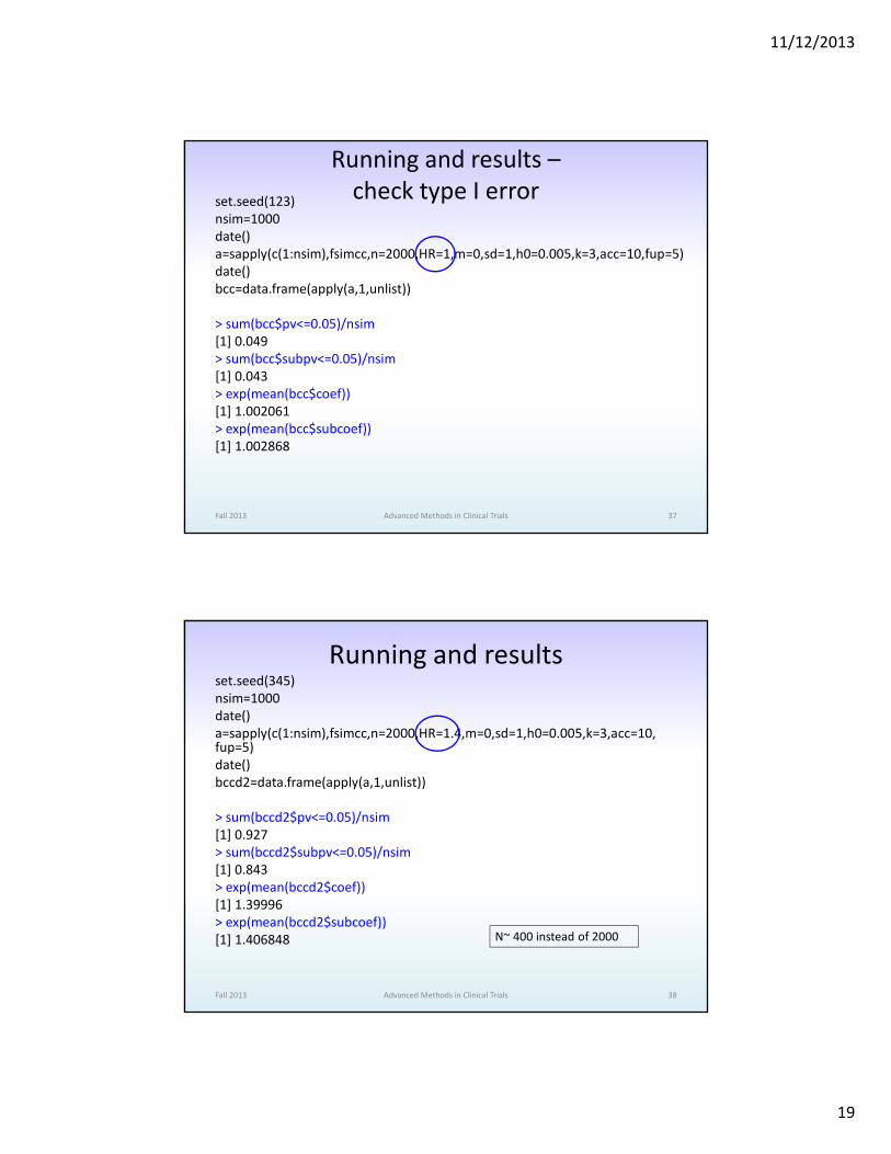
Running and results –

check type I errorset.seed(123)

nsim=1000

date()

a=sapply(c(1:nsim),fsimcc,n=2000,HR=1,m=0,sd=1,h0=0.005,k=3,acc=10,fup=5)

date()

bcc=data.frame(apply(a,1,unlist))

> sum(bcc$pv<=0.05)/nsim

[1] 0.049

> sum(bcc$subpv<=0.05)/nsim

[1] 0.043

> exp(mean(bcc$coef))

[1] 1.002061

> exp(mean(bcc$subcoef))

[1] 1.002868


Running and resultsset.seed(345)

nsim=1000

date()

a=sapply(c(1:nsim),fsimcc,n=2000,HR=1.4,m=0,sd=1,h0=0.005,k=3,acc=10,fup=5)

date()

bccd2=data.frame(apply(a,1,unlist))

> sum(bccd2$pv<=0.05)/nsim

[1] 0.927

> sum(bccd2$subpv<=0.05)/nsim

[1] 0.843

> exp(mean(bccd2$coef))

[1] 1.39996

> exp(mean(bccd2$subcoef))

[1] 1.406848


N~ 400 instead of 2000

11/12/2013

20

• library(cmprsk)

• plot.cuminc=getS3method(‘plot’,’cuminc’)


Fall 2013 40

Definition

Competing risks type of event=

the event whose occurrence either

precludes the occurrence of another

event under investigation or

fundamentally alters the probability of

occurrence of this other event.

Gooley, TA; Leisenring, W; Crowley, J; Storer, BE, "Estimation of failure probabilities in the presence of competing risks: new representations of old estimators" Statistics in Medicine 1999 pp. 695-706


11/12/2013

21

Fall 2013 41

Definition, Examples

• Death: due to disease (MI) and due to

other causes

• First relapse: local relapse and distant

relapse

the event whose occurrence either precludes the

occurrence of another event under investigation

fundamentally alters the probability of occurrence of this other event


Fall 2013 42

Examples

• To study the time to failure (any type) in a group of cancer patients

– Relapse

– Deaths

• To study cause specific survival

– Deaths of the disease

– Other deaths

• Study late side effects of chemotherapy


11/12/2013

22

• In competing risks setting we can observe only one event of multiple possible events.

• Example

– Death of disease vs. other deaths

– Relapse vs. death before relapse

• Number of events is important for the sample size/power calculation

• Cannot ignore the existence of CR events (cannot censor the CR events).


Fall 2013 44

Analysis

• To estimate the probability of event: a modification of the K-M technique = cumulative incidence function (CIF)

• The probability of event is not a proper distribution – sub-distribution

• Modelling: a modification of the Cox proportional hazards model = Fine and Gray model (models the hazard of the sub-distribution=sub-distribution hazard)

• The effects are expressed similarly – hazard ratio, hazard=sub-distribution hazard.


11/12/2013

23

Fall 2013 45

Sample size calculation (CR)

1 / 2 1( )

ln( )ev

z zn

HRα β

σ− −+

=

ev

ev

nN

P=

( ) ( ) ( )

1( )

ev cr ev crf f a

evev

ev cr ev cr

e eP

a

λ λ λ λλλ λ λ λ

− + × − + × + −= × − + + ×

Assumption: Exponential distribution, independence

( )

1ev evf f a

ev

ev

e eP

a

λ λ

λ

− − +−= −


HR= refers to the ratio

of the sub-distribution

hazards

Fall 2013 46

0.0 0.2 0.4 0.6 0.8

0.1

0.2

0.3

0.4

0.5

0.6

Decrease of Pev as λcr increases

Hazard rate for competing risk

Pro

babi

lity

of e

vent

, Pev

Pevwhen no competing risks


11/12/2013

24

A general power calculation

• A randomized clinical trial (stomach)

• Standard RT vs. another type of RT

• Local failure (stomach)

• Parameters and assumptions:

– Time to local failure ~ Exponential: λS=0.4, λE=0.2

– Time to CR (death or other failures): Exp: λCR =0.1

– The intervention has no effect on CR

– Accrual time over 5 years. 1 year extra follow-up

– Accrual rate = 40 patients/year

– Equal number of patients in the 2 arms

Fall 2013 47Advanced Methods in Clinical Trials

Instead of giving the 2

hazards rates one may

have the HR of the

sub-distributions.


Fall 2013 48

1 / 2 1( )

ln( )ev

z zn

HRα β

σ− −+

=5 = 0.05, 7�89 �` = 1.96E = 0.2, 7�8F = 0.84� = 1 2̀

�� = �-ab�-ac

�-ab = �� 1 − NbNb + Nde 1 − �8(Pf/Pgh)R

�-ac = �� 1 − NcNc + Nde 1 − �8(Pi/Pgh)R

Basically, we do not have proportional hazards. HR~1.9

Required number of events = 76


0 1 2 3 4 5 6

1.75

1.80

1.85

1.90

1.95

2.00

Time

Sub

dist

ribut

ion

HR

11/12/2013

25


Fall 2013 49

( ) ( ) ( )

1( )

ev cr ev crf f a

evev

ev cr ev cr

e eP

a

λ λ λ λλλ λ λ λ

− + × − + × + −= × − + + ×

ev

ev

nN

P=

Apply this for each arm

Probability of event for the duration of the study is 0.6 for standard and 0.4

for the experimental. Approximately the probability of event is 0.5

It follows that the total number of patients needed to be able to

observe 76 events is 152. Since the accrual rate is 40/year then

the assumed accrual time of 5 years is reasonable but long.

As a consequence, some patients will not have as much follow-up as

assumed:

- Instead of 1-6 years

- Will be 1-4.8 years

Recommendation: to increase the follow-up from 1 years to 2 years.

P=0.56 => N=134 => with 152 a slightly larger power.


How to estimate the hazard rates for

standard arm

• In the literature the estimates for relapse rate

will very likely be based on the Kaplan-Meier

methodology (censoring the competing risks).

• N = − ejeklR where t is the time at which the

estimate was calculated.


11/12/2013

26

Fall 2013 51

How to estimate the hazard rates for

standard arm

If the estimates are based on the cumulative incidence function approach ( CIF or )

( )( )( )( )( )

0

0

0 0

ˆlogˆ

ˆ1ev ev

S tF t

t S tλ

−= ×

−

F̂

( )( )( )( )( )

0

0

0 0

ˆlogˆ

ˆ1cr cr

S tF t

t S tλ

−= ×

−

( ) ( ) ( )0 0 0ˆ ˆ ˆ1 ev crS t F t F t= − −


Example of code for simulation when CRfsimcr=function(i,yearrate,

lambda1ev,lambda2ev,

lambda1cr,lambda2cr,f,a)

{

ntotal=a*yearrate

n=ceiling(ntotal/2)

timeev1=rexp(n,lambda1ev)

timeev2=rexp(n,lambda2ev)


timecr1=rexp(n,lambda1cr)

timecr2=rexp(n,lambda2cr)

timecr=c(timecr1,timecr2)

timecensor=runif((2*n),f,(f+a))

time=apply(cbind(timeev,timecr,timecensor),

1,min)

event=(time==timeev)+2*(time==timecr)

x=c(rep(1,n),rep(0,n))

numev=sum(event==1)

numcr=sum(event==2)

fitcrr=crr(time,event,x)

fitcif=cuminc(time,event,x)

coef=fitcrr$coef

est=timepoints(fitcif,times=5)$est[1:2]

pvwald=summary(fitcrr)$coef[5]

pvgray=fitcif$Tests[3]

out=data.frame(n,coef,numev,numcr,

estlowrisk=est[1],esthighrisk=est[2],

pvwald,pvgray)

print(i)

return(out)}


11/12/2013

27

Example of code for simulation when CRset.seed(123)

nsim=10000

date()

a=sapply(c(1:nsim),fsimcr,yearrate=40,lambda1ev=0.4,lambda2ev=0.2,lambda1cr=0.1,lambda2cr=0.1,f=2,a=3.8)

date()

bcr=data.frame(apply(a,1,unlist))

head(bcr)

> sum(bcr$pvwald<=0.05)/nsim

[1] 0.8478

> sum(bcr$pvgray<=0.05)/nsim

[1] 0.8468

> exp(mean(bcr$coef))

[1] 1.909454

> summary(bcr$estlowrisk)

Min. 1st Qu. Median Mean 3rd Qu. Max. NA' s 0.2545 0.4687 0.5162 0.5169 0.5634 0.7817 243 > summary(bcr$esthighrisk)

Min. 1st Qu. Median Mean 3rd Qu. Max. NA' s 0.4859 0.6835 0.7245 0.7228 0.7637 0.9325 2 716 > summary(bcr$numev)

Min. 1st Qu. Median Mean 3rd Qu. Max. 61.00 81.00 85.00 84.95 89.00 106.00


How can one decide the number of

simulations?

• Decide on a number of simulations which is

reasonable time wise.

• Run it twice, each time using a different seed.

• If the results are quite different than you have

to increase the number of simulations


11/12/2013

28

Conclusion

• The sample size calculation could be time consuming but very important

• Need to take the time to do it correctly.

– We want to minimize the number of patients exposed to an inferior treatment.

– We do not want to discard a potential superior treatment

• The results should be translated such that the PI understands the magnitude of the effect size to be detected


power and sample size for time to event - andrew · pdf file11/12/2013 3 the extent of...

Documents