Statistical Techniques IEXST7005

Sample Size Calculation

The sample size formula

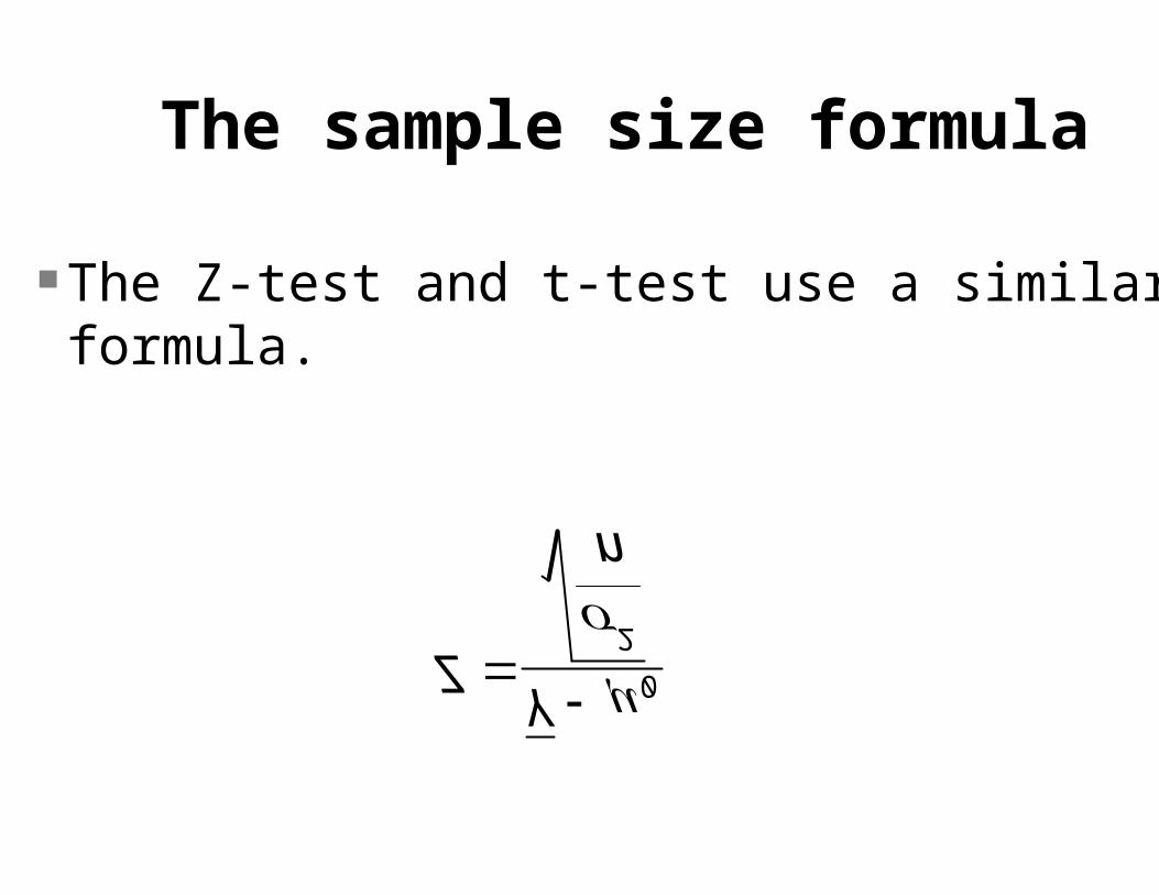
The Z-test and t-test use a similar formula.

The sample size formula (continued)

Lets suppose we know everything in the formula except n. Do we really? Maybe not, but we can get some pretty good estimates.

Call the numerator (Y - 0) a difference, d. It is some mean difference we want to be able to detect, so d = Y - 0.

The value 2 is a variance, the variance of the data that we will be sampling. We need this variance, or an estimate, S2.

The sample size formula (continued)

So we alter the formula to read.

The sample size formula (continued)

What other values do we know? Do we know Z? No, but we know what Z we need to obtain significance. If we are doing a 2-tailed test, and we set = 0.05, then Z will be 1.96.

Any calculated value larger will be "more significant", any value smaller will not be significant.

So, if we want to detect significance at the 5% level, we can state that ...

The sample size formula (continued)

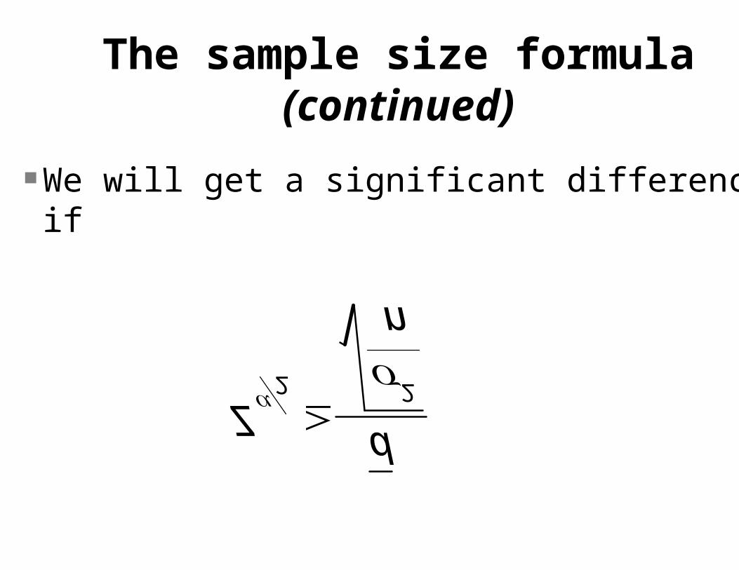
We will get a significant difference if

The sample size formula (continued)

We square both sides and solve for n. Then we will also get a significant difference if

The sample size formula (continued)

Then, if we have an idea of values for d, 2, and Z, we can solve the formula for n.If we are going to use a Z distribution we should

have a known value of the variance (2). If the variance is calculated from the sample, use the t distribution.

This would give us the sample size needed to obtain "significance", in accordance with whatever Z value is chosen.

Generic Example Try an example where

d = 2 2 = 5 Z = 1.96

So what value of n would detect this difference with this variance and produce a value of Z equal to 1.96 (or greater)? n (Z22)/d2 = (1.962 * 52)/22 = 3.8416(25)/4 =

24.01since n 24.01, round up to 25.

Generic Example (continued) Answer, n 25 would produce significant results.

Guaranteed? Wouldn't this always produce significant results?

Theoretically, within the limits of statistical probability of error, yes. But only IF THE DIFFERENCE WAS REALLY 2.

If the null hypothesis (no difference,Y-0=0) was really true and we took larger samples, then we would get a better estimate of 0, and may never show significance.

Considering Type II Error

The formula we have seen contains only Z/2 or t/2, depending on whether we have 2 or S2. However, a fuller version can contain consideration of the probability of Type II error ().

Remember that to work with we need to know the mean of the real distribution. However, in calculating sample size we have a difference,d = Y - 0. So we can include consideration of type II error.

Considering Type II Error (continued)

error consideration would be done by adding another Z or t for the error rate. Notice that below I switch to t distributions and use S2.

Other examples

We have done a number of tests, some yielding significant results and others not. If a test that yields significant results (showing a

significant difference between the observed and hypothesized values), then we don't need to examine sample size because the sample was big enough.

However, some utility may be made of this information if we FAIL to reject the null hypothesis.

An example with t values and error included

Recall the Rhesus monkey experiment. We hypothesized no effect of a drug, and with a sample size of 10 were unable to reject the null hypothesis. However, we did observe a difference of +0.8

change in blood pressure after administering the drug.

What if this change was real? What if we made a Type II error? How large a sample would we need to test for a difference of 0.8 if we also wanted 90% power?

An example with t values and error included (continued)

So we want to know how large a sample we would need to get significance at the =0.05 level if power was 0.90. In this case =0.10. To do this calculation we need a two tailed and a one tailed (we know that the change is +0.8).

We will estimate the variance from the sample so we will use the t distribution. However, since we don't know the sample size we don't know the d.f.!

An example with t values and error included (continued)

So we will approximate to start with. Given the information,

= 0.05 so t will be approximately 2 = 0.10 so t will be roughly 1.3 d =Y-0 = 0.8 from our previous results, and S2 = 9.0667 from our previous results.

An example with t values and error included (continued)

We do the calculations.

And now we have an estimate of n and the degrees of freedom. n = 155 and d.f.=154. We can refine our values for t/2 and tfor d.f. = 154, t/2 = 1.97 approx.for d.f. = 154, t = 1.287 approx.

An example with t values and error included (continued)

So we redo the calculations with improved estimates.

A little improvement. If we saw much change in the estimate of n, we could recalculate as often as necessary. Usually 3 or 4 recalculations is enough.

Summary

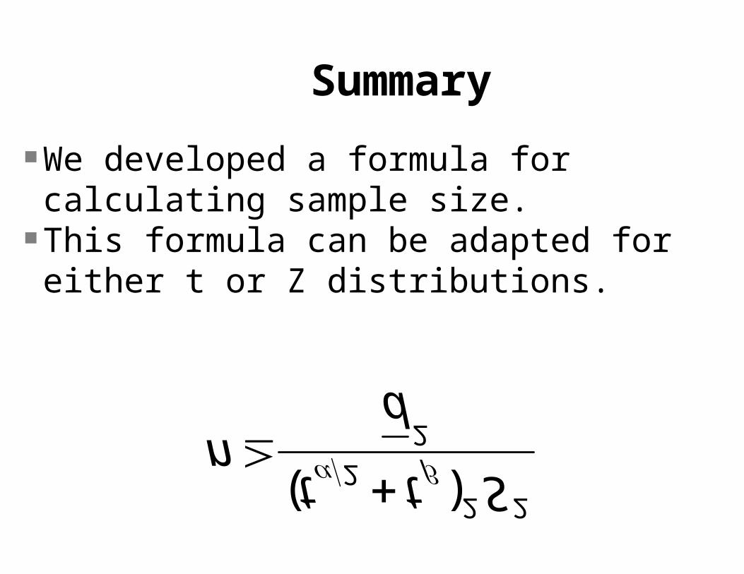
We developed a formula for calculating sample size.

This formula can be adapted for either t or Z distributions.

Summary (continued) We learned that We need input values of

, , S2 (or 2) and we need to know what difference we want to

detect (d).

Summary (continued)

We saw that for the t-test, the first calculation was only approximate since we didn't know the degrees of freedom and could not get the appropriate value of t.

However, after the initial calculation the estimate could be improved by iteratively recalculating the estimate of the value of n until it was stable.