poset topology: tools and applications - department of mathematics
TRANSCRIPT

Poset Topology: Tools and Applications
Michelle L. Wachs
IAS/Park City Mathematics Institute, Summer 2004

Contents
Poset Topology: Tools and Applications 1
Introduction 3
Lecture 1. Basic definitions, results, and examples 51.1. Order complexes and face posets 51.2. The Mobius function 91.3. Hyperplane and subspace arrangements 111.4. Some connections with graphs, groups and lattices 161.5. Poset homology and cohomology 171.6. Top cohomology of the partition lattice 19
Lecture 2. Group actions on posets 232.1. Group representations 232.2. Representations of the symmetric group 252.3. Group actions on poset (co)homology 302.4. Symmetric functions, plethysm, and wreath product modules 32
Lecture 3. Shellability and edge labelings 413.1. Shellable simplicial complexes 413.2. Lexicographic shellability 453.3. CL-shellability and Coxeter groups 573.4. Rank selection 62
Lecture 4. Recursive techniques 674.1. Cohen-Macaulay complexes 674.2. Recursive atom orderings 714.3. More examples 734.4. The Whitney homology technique 774.5. Bases for the restricted block size partition posets 824.6. Fixed point Mobius invariant 90
Lecture 5. Poset operations and maps 915.1. Operations: Alexander duality and direct product 915.2. Quillen fiber lemma 955.3. General poset fiber theorems 1005.4. Fiber theorems and subspace arrangements 1035.5. Inflations of simplicial complexes 105
Bibliography 1092

IAS/Park City Mathematics SeriesVolume 00, 2004
Poset Topology: Tools and Applications
Michelle L. Wachs
Introduction
The theory of poset topology evolved from the seminal 1964 paper of Gian-CarloRota on the Mobius function of a partially ordered set. This theory provides a deepand fundamental link between combinatorics and other branches of mathematics.Early impetus for this theory came from diverse fields such as
• commutative algebra (Stanley’s 1975 proof of the upper bound conjecture)• group theory (the work of Brown (1974) and Quillen (1978) on p-subgroup
posets)• combinatorics (Bjorner’s 1980 paper on poset shellability)• representation theory (Stanley’s 1982 paper on group actions on the ho-
mology of posets)• topology (the Orlik-Solomon theory of hyperplane arrangements (1980))• complexity theory (the 1984 paper of Kahn, Saks, and Sturtevant on the
evasiveness conjecture).Later developments have kept the theory vital. I mention just a few examples:Goresky-MacPherson formula for subspace arrangements, Bjorner-Lovasz-Yao com-plexity theory results, Bjorner-Wachs extension of shellability to nonpure com-plexes, Forman’s discrete version of Morse theory, and Vassiliev’s work on knotinvariants and graph connectivity.
So, what is poset topology? By the topology of a partially ordered set (poset)we mean the topology of a certain simplicial complex associated with the poset,called the order complex of the poset. In these lectures I will present some ofthe techniques that have been developed over the years to study the topology of aposet, and discuss some of the applications of poset topology to the fields mentionedabove as well as to other fields. In particular, I will discuss tools for computinghomotopy type and (co)homology of posets, with an emphasis on group equivariant(co)homology. Although posets and simplicial complexes can be viewed as essen-tially the same topological object, we will narrow our focus, for the most part,
Department of Mathematics, University of Miami, Coral Gables, Fl 33124.E-mail address: [email protected] work was partially supported by NSF grant DMS 0302310.
c©2004 Michelle L. Wachs
3

4 WACHS, POSET TOPOLOGY
to tools that were developed specifically for posets; for example, lexicographicalshellability, recursive atom orderings, Whitney homology techniques, (co)homologybases/generating set techniques, and fiber theorems.
Research in poset topology is very much driven by the study of concrete ex-amples that arise in various contexts both inside and outside of combinatorics.These examples often turn out to have a rich and interesting topological struc-ture, whose analysis leads to the development of new techniques in poset topology.These lecture notes are organized according to techniques rather than applications.A recurring theme is the use of original examples in demonstrating a technique,where by original example I mean the example that led to the development of thetechnique in the first place. More recent examples will be discussed as well.
With regard to the choice of topics, I was primarily motivated by my ownresearch interests and the desire to provide the students at the PCMI graduateschool with concrete skills in this subject. Due to space and time constraints andmy decision to focus on techniques specific to posets, there are a number of veryimportant tools for general simplicial complexes that I have only been able tomention in passing (or not at all). I point out, in particular, discrete Morse theory(which is a major part of the lecture series of Robin Forman, its originator) andbasic techniques from algebraic topology such as long exact sequences and spectralsequences. For further techniques and applications, still of current interest, westrongly recommend the influential 1995 book chapter of Anders Bjorner [29].
The exercises vary in difficulty and are there to reinforce and supplement thematerial treated in these notes. There are many open problems (simply referred toas problems) and conjectures sprinkled throughout the text.
I would like to thank the organizers (Ezra Miller, Vic Reiner and Bernd Sturm-fels) of the 2004 PCMI Graduate Summer School for inviting me to deliver theselectures. I am very grateful to Vic Reiner for his encouragement and support. Iwould also like to thank Tricia Hersh for the help and support she provided as myoverqualified teaching assistant. Finally, I would like to express my gratitude tothe graduate students at the summer school for their interest and inspiration.

LECTURE 1Basic definitions, results, and examples
1.1. Order complexes and face posets
We begin by defining the order complex of a poset and the face poset of a simplicialcomplex. These constructions enable us to view posets and simplicial complexes asessentially the same topological object. We shall assume throughout these lecturesthat all posets and simplicial complexes are finite, unless otherwise stated.
An abstract simplicial complex ∆ on finite vertex set V is a nonempty collectionof subsets of V such that
• {v} ∈ ∆ for all v ∈ V• if G ∈ ∆ and F ⊆ G then F ∈ ∆.
The elements of ∆ are called faces (or simplices) of ∆ and the maximal facesare called facets. We say that a face F has dimension d and write dimF = d ifd = |F | − 1. Faces of dimension d are referred to as d-faces. The dimension dim ∆of ∆ is defined to be maxF∈∆ dimF . We also allow the (-1)-dimensional complex{∅}, which we refer to as the empty simplicial complex. It will be convenient to referto the empty set ∅, as the degenerate empty complex and say that it has dimension−2, even though we don’t really consider it to be a simplicial complex. If all facetsof ∆ have the same dimension then ∆ is said to be pure.
A d-dimensional geometric simplex in Rn is defined to be the convex hull of d+1affinely independent points in Rn called vertices. The convex hull of any subset ofthe vertices is called a face of the geometric simplex. A geometric simplicial complexK in Rn is a nonempty collection of geometric simplices in Rn such that
• Every face of a simplex in K is in K.• The intersection of any two simplices of K is a face of both of them.
From a geometric simplicial complex K, one gets an abstract simplicial com-plex ∆(K) by letting the faces of ∆(K) be the vertex sets of the simplices of K.Every abstract simplicial complex ∆ can be obtained in this way, i.e., there is ageometric simplicial complex K such that ∆(K) = ∆. Although K is not unique,the underlying topological space, obtained by taking the union of the simplices ofK under the usual topology on Rn, is unique up to homeomorphism. We refer tothis space as the geometric realization of ∆ and denote it by ‖∆‖. We will usually
5

6 WACHS, POSET TOPOLOGY
1
2
3
4
5 6
P
1
2
3
54
6
∆∆∆∆((((P)
Figure 1.1.1. Order complex of a poset
1
2
3
4
∆∆∆∆
1 2 3 4
12 13 23 34
123
PPPP((((∆∆∆∆))))
1 2 3 4
12 13 23 34
123
LLLL((((∆∆∆∆))))
^0
^1
Figure 1.1.2. Face poset and face lattice of a simplicial complex
drop the ‖ ‖ and let ∆ denote an abstract simplicial complex as well as its geometricrealization.
To every poset P , one can associate an abstract simplicial complex ∆(P ) calledthe order complex of P . The vertices of ∆(P ) are the elements of P and the facesof ∆(P ) are the chains (i.e., totally ordered subsets) of P . (The order complexof the empty poset is the empty simplicial complex {∅}.) For example, the Hassediagram of a poset P and the geometric realization of its order complex are givenin Figure 1.1.1.
To every simplicial complex ∆, one can associate a poset P (∆) called the faceposet of ∆, which is defined to be the poset of nonempty faces ordered by inclusion.The face lattice L(∆) is P (∆) with a smallest element 0 and a largest element 1attached. An example is given in Figure 1.1.2.

LECTURE 1. BASIC DEFINITIONS, RESULTS, AND EXAMPLES 7
1 2 3 4
1
2
3
4
∆∆∆∆
12 13 23 34
123
PPPP((((∆∆∆∆))))
1
2
3
4
∆∆∆∆((((PPPP((((∆∆∆∆))))))))
12312
13
23
34
Figure 1.1.3. Barycentric subdivision
1 2 3
12 13 23
1
2
3
12
13
23
B3
∆∆∆∆((((B3)
Figure 1.1.4. Order complex of the subset lattice (Boolean algebra)
If we start with a simplicial complex ∆, take its face poset P (∆), and then takethe order complex ∆(P (∆)), we get a simplicial complex known as the barycentricsubdivision of ∆; see Figure 1.1.3. The geometric realizations are always homeo-morphic,
∆ ∼= ∆(P (∆)).When we attribute a topological property to a poset, we mean that the geomet-
ric realization of the order complex of the poset has that property. For instance, ifwe say that the poset P is homeomorphic to the n-sphere Sn we mean that ‖∆(P )‖is homeomorphic to Sn.
Example 1.1.1. The Boolean algebra. Let Bn denote the lattice of subsets of[n] := {1, 2, . . . , n} ordered by containment, and let Bn := Bn − {∅, [n]}. Then
Bn∼= Sn−2
because ∆(Bn) is the barycentric subdivision of the boundary of the (n−1)-simplex.See Figure 1.1.4.
We now review some basic poset terminology. An m-chain of a poset P is atotally ordered subset c = {x1 < x2 < · · · < xm+1} of P . We say the length l(c) ofc is m. We consider the empty chain to be a (−1)-chain. The length l(P ) of P is

8 WACHS, POSET TOPOLOGY
defined to be
l(P ) := max{l(c) : c is a chain of P}.Thus, l(P ) = dim ∆(P ) and l(P (∆)) = dim ∆.
A chain of P is said to be maximal if it is inclusionwise maximal. Thus, the setM(P ) of maximal chains of P is the set of facets of ∆(P ). A poset P is said to bepure (also known as ranked or graded) if all maximal chains have the same length.Thus, P is pure if and only if ∆(P ) is pure. Also a simplicial complex ∆ is pureif and only if its face poset P (∆) is pure. The posets and simplicial complexes ofFigures 1.1.1 and 1.1.2 are all nonpure, while the poset and simplicial complex ofFigure 1.1.4 are both pure.
For x ≤ y in P , let (x, y) denote the open interval {z ∈ P : x < z < y} and let[x, y] denote the closed interval {z ∈ P : x ≤ z ≤ y}. Half open intervals (x, y] and[x, y) are defined similarly.
If P has a unique minimum element, it is usual to denote it by 0 and referto it as the bottom element. Similarly, the unique maximum element, if it exists,is denoted 1 and is referred to as the top element. Note that if P has a bottomelement 0 or top element 1 then ∆(P ) is contractible since it is a cone. We usuallyremove the top and bottom elements and study the more interesting topology ofthe remaining poset. Define the proper part of a poset P , for which |P | > 1, to be
P := P − {0, 1}.
In the case that |P | = 1, it will be convenient to define ∆(P ) to be the degenerateempty complex ∅. We will also say ∆((x, y)) = ∅ and l((x, y)) = −2 if x = y.
For posets with a bottom element 0, the elements that cover 0 are called atoms.For posets with a top element 1, the elements that are covered by 1 are calledcoatoms.
A poset P is said to be bounded if it has a top element 1 and a bottom element0. Given a poset P , we define the bounded extension
P := P ∪ {0, 1},
where new elements 0 and 1 are adjoined (even if P already has a bottom or topelement).
A poset P is said to be a meet semilattice if every pair of elements x, y ∈ Phas a meet x∧ y, i.e. an element less than or equal to both x and y that is greaterthan all other such elements. A poset P is said to be a join semilattice if everypair of elements x, y ∈ P has a join x ∨ y, i.e. a unique element greater than orequal to both x and y that is less than all other such elements. If P is both a joinsemilattice and a meet semilattice then P is said to be a lattice. It is a basic fact oflattice theory that any finite meet (join) semilattice with a top (bottom) elementis a lattice.
The dual of a poset P is the poset P ∗ on the same underlying set with theorder relation reversed. Topologically there is no difference between a poset and itsdual since ∆(P ) and ∆(P ∗) are identical simplicial complexes. The direct productP × Q of two posets P and Q is the poset whose underlying set is the cartesianproduct {(p, q) : p ∈ P, q ∈ Q} and whose order relation is given by
(p1, q1) ≤P×Q (p2, q2) if p1 ≤P p2 and q1 ≤Q q2.

LECTURE 1. BASIC DEFINITIONS, RESULTS, AND EXAMPLES 9
1
-1 -1 -1
1 1 2
-2
-1
1
Figure 1.2.1. µ(0, x)
Define the join of two simplicial complexes ∆ and Γ on disjoint vertex sets tobe the simplicial complex given by
∆ ∗ Γ := {A ∪ B : A ∈ ∆, B ∈ Γ}.(1.1.1)
The join (or ordinal sum) P ∗ Q of posets P and Q is the poset whose underlyingset is the disjoint union of P and Q and whose order relation is given by x < y ifeither (i) x <P y, (ii) x <Q y, or (iii) x ∈ P and y ∈ Q. Clearly
∆(P ∗ Q) = ∆(P ) ∗ ∆(Q).
There are topological relationships between the join and product of posets, whichare discussed in Section 5.1.
1.2. The Mobius function
The story of poset topology begins with the Mobius function µ(= µP ) of a posetP defined recursively on closed intervals of P as follows:
µ(x, x) = 1, for all x ∈ P
µ(x, y) = −∑
x≤z<y
µ(x, z), for all x < y ∈ P.
For a bounded poset P , define the Mobius invariant
µ(P ) := µP (0, 1).
In Figure 1.2.1, the values of µ(0, x) are shown for each element x of the poset.There are various techniques for computing the Mobius function of a poset; see
[169]. Perhaps the most basic technique is given by the product formula.
Proposition 1.2.1. Let P and Q be posets. Then for (p1, q1) ≤ (p2, q2) ∈ P × Q,
µP×Q((p1, q1), (p2, q2)) = µP (p1, p2)µQ(q1, q2).
Exercise 1.2.2. Prove Proposition 1.2.1.
Exercise 1.2.3. Use the product formula to show that the Mobius function forthe subset lattice Bn is given by
µ(X, Y ) = (−1)|Y −X| for all X ⊆ Y.

10 WACHS, POSET TOPOLOGY
Exercise 1.2.4. For positive integer n, the lattice Dn of divisors of n is the setof positive divisors of n ordered by a ≤ b if a divides b. Show that the Mobiusfunction for Dn is given by
µ(d, m) = µ(m/d),where µ(·) is the classical Mobius function of number theory, which is defined onthe set of positive integers by
µ(n) =
{(−1)k if n is the product of k distinct primes0 if n is divisible by a square.
This example is the reason for the name Mobius function of a poset.
The combinatorial significance of the Mobius function was first demonstratedby Rota in 1964 in his Steele-prize winning paper [147]. The Mobius function of aposet is used in enumerative combinatorics to obtain inversion formulas.
Proposition 1.2.5 (Mobius inversion). Let P be a poset and let f, g : P → C.Then
g(y) =∑x≤y
f(x)
if and only iff(y) =
∑x≤y
µ(x, y) g(x).
Three examples of Mobius inversion are classical Mobius inversion (P = Dn),inclusion-exclusion (P = Bn), and Gaussian inversion (P = Bn(q), the lattice ofsubspaces of an n-dimensional vector space over the field with q elements); see [169]for details.
Our interest in the Mobius function stems from its connection to the Eulercharacteristic. The reduced Euler characteristic χ(∆) of a simplicial complex ∆ isdefined to be
χ(∆) :=dim ∆∑i=−1
(−1)i fi(∆),
where fi(∆) is the number of i-faces of ∆.
Proposition 1.2.6 (Philip Hall Theorem). For any poset P ,
µ(P ) = χ(∆(P )).
Exercise 1.2.7. Prove Proposition 1.2.6.
It follows from the Euler-Poincare formula below that the Euler characteristicis a topological invariant. Hence by Proposition 1.2.6, µP (x, y) depends only onthe topology of the open interval (x, y) of P .
Theorem 1.2.8 (Euler-Poincare formula). For any simplicial complex ∆,
χ(∆) :=dim ∆∑i=−1
(−1)i βi(∆),
where βi(∆) is the ith reduced Betti number of ∆, i.e., the rank, as an abeliangroup, of the ith reduced homology of ∆ over Z.

LECTURE 1. BASIC DEFINITIONS, RESULTS, AND EXAMPLES 11
12
3 4
56
7 8
A
21 3 4
76
0
5 8
L(A)
Figure 1.3.1. Intersection semilattice of a hyperplane arrangement
The Mobius function of a poset plays a fundamental role in the theory ofhyperplane arrangements and the homology of a poset plays a fundamental role inthe theory of subspace arrangements. We discuss the connection with arrangementsin the next section.
1.3. Hyperplane and subspace arrangements
A hyperplane arrangement A is a finite collection of (affine) hyperplanes in somevector space V . We will consider only real hyperplane arrangements (V = Rn) andcomplex hyperplane arrangements (V = Cn) here.
Real hyperplane arrangements divide Rn into regions. A remarkable formulafor the number of regions was given by Zaslavsky [213] in 1975. This formulainvolves the notion of intersection semilattice of a hyperplane arrangement.
The intersection semilattice L(A) of a hyperplane arrangement A is defined tobe the meet semilattice of nonempty intersections of hyperplanes in A ordered byreverse inclusion. Note that we include the intersection over the empty set whichis the bottom element 0 of L(A). Note also that L(A) has a top element if andonly if ∩A = ∅. Such an arrangement is called a central arrangement. Hence forcentral arrangements A, the intersection semilattice L(A) is actually a lattice. Anexample of a hyperplane arrangement in R2 and its intersection semilattice aregiven in Figure 1.3.1.
Before stating Zaslavsky’s formula, we discuss four fundamental examples ofreal hyperplane arrangements and their intersection lattices, to which we referthroughout these lectures.
Example 1.3.1. The (type A) coordinate hyperplane arrangement and the Booleanalgebra Bn. The coordinate hyperplane arrangement is the central hyperplanearrangement consisting of the coordinate hyperplanes xi = 0 in Rn. It is easy tosee that the intersection lattice of this arrangement is isomorphic to the subsetlattice Bn. Indeed, the intersection
{x ∈ Rn : xi1 = xi2 = · · · = xik= 0},
where 1 ≤ i1 < i2 < · · · < ik ≤ n, corresponds to the subset {i1, i2, . . . , ik}. Thiscorrespondence is an isomorphism from the intersection lattice to Bn.
Example 1.3.2. The type B coordinate hyperplane arrangement and the face latticeof the n-cross-polytope Cn. The type B coordinate hyperplane arrangement is the

12 WACHS, POSET TOPOLOGY
12/3 13/2 23/1
123
1/2/3
x1 = x 3x2 = x 3
x1 = x 2
A2 L(A2)=Π3
Figure 1.3.2. Intersection lattice of braid arrangement
affine hyperplane arrangement consisting of the hyperplanes xi = ±1 in Rn. Onecan see that if we attach a top element 1 to the intersection semilattice of thisarrangement we have a lattice that is isomorphic to the lattice of faces of the n-cross-polytope, which we denote by Cn. (This is dual to the lattice of faces of then-cube.) Indeed, the intersection
{x ∈ Rn : ε1xi1 = ε2xi2 = · · · = εkxik= 1},
where 1 ≤ i1 < i2 < · · · < ik ≤ n and εi ∈ {−1, 1}, maps to the (n − k)-face
{x ∈ [−1, 1]n : ε1xi1 = ε2xi2 = · · · = εkxik= 1}
of the n-cube. This correspondence is an isomorphism from the intersection latticeto the dual of the face lattice of the cube.
Example 1.3.3. The (type A) braid arrangement and the partition lattice Πn. For1 ≤ i < j ≤ n, let
Hi,j = {x ∈ Rn : xi = xj}.The hyperplane arrangement
An−1 := {Hi,j : 1 ≤ i < j ≤ n}is known as the braid arrangement or the type A Coxeter arrangement. The in-tersection lattice L(An−1) is isomorphic to Πn, the lattice of partitions of the set[n] ordered by refinement. Indeed, for each partition π ∈ Πn, let �π be the linearsubspace of Rn consisting of all points (x1, . . . , xn) such that xi = xj whenever iand j are in the same block of π. The map π �→ �π is a poset isomorphism from Πn
to L(An−1). The braid arrangement A2 intersected with the plane x1 +x2 +x3 = 0and the partition lattice Π3 are shown in Figure 1.3.2.
Example 1.3.4. The type B braid arrangement and the type B partition latticeΠB
n . For 1 ≤ i < j ≤ n, let
H+i,j = {x ∈ Rn : xi = xj} and H−
i,j = {x ∈ Rn : xi = −xj}.For i = 1, . . . n, let
Hi = {x ∈ Rn : xi = 0}.

LECTURE 1. BASIC DEFINITIONS, RESULTS, AND EXAMPLES 13
01/2 02/1 0/12
012
0/1/2
L(B2)=Π2B
x1 = -x2x1 = 0
B2
x1 = x2
x2 = 0 0/12
Figure 1.3.3. Intersection lattice of type B braid arrangement
The hyperplane arrangement
Bn := {H+i,j : 1 ≤ i < j ≤ n} ∪ {H−
i,j : 1 ≤ i < j ≤ n} ∪ {Hi : 1 ≤ i ≤ n}is called the type B braid arrangement or the type B Coxeter arrangement. Theintersection lattice L(Bn) is isomorphic to the type B (or signed) partition lattice.The elements of the type B partition lattice ΠB
n are partitions of {0, . . . , n} forwhich any of the elements of [n] can have a bar except for the elements of the blockthat contains 0 and the smallest element of each block. For example, 025/179/3468is an element of ΠB
9 , while 025/179/3468 is not because 5 and 3 are not allowedto be barred. The covering relation is given by π1 <·π2 if π2 is obtained from π1
by merging two blocks B1 and B2 into a single block B in the following manner:Suppose minB1 < minB2. Then
• if 0 ∈ B1, let B be the union of B1 and B2 with all bars removed,• if 0 /∈ B1, let B be the union of either
– B1 and B2 with all bars intact or– B1 and B2, where B2 is obtained from B2 by barring all unbarred
elements and unbarring all barred elements.For example, the type B partitions that cover 025/179/3468 in ΠB
9 are
012579/3468, 0234568/179, 025/1346789, 025/1346789.
The isomorphism from ΠBn to L(Bn) is quite natural. Take a typical type B partition
025/179/3468.
It maps to the subspace
{x ∈ R9 : x2 = x5 = 0, x1 = −x7 = x9, x3 = x4 = −x6 = −x8},in L(Bn). The type B braid arrangement B2 and the type B partition lattice ΠB
2
are shown in Figure 1.3.3.
Examples 1.3.1 and 1.3.3 are referred to as type A examples, and Examples 1.3.2and 1.3.4 are referred to as type B examples because of their connection withCoxeter groups. Indeed, associated with every finite Coxeter group (i.e., finitegroup generated by Euclidean reflections) is a simplicial complex called its Coxetercomplex. The order complex of the Boolean algebra Bn is the Coxeter complex
14 WACHS, POSET TOPOLOGY
of the symmetric group Sn, which is the type A Coxeter group, and the ordercomplex of the face lattice of the cross-polytope Cn is the Coxeter complex of thehyperoctahedral group, which is the type B Coxeter group. (The use of notation isunfortunate here; Bn is type A and Cn is type B.)
Also associated with every finite Coxeter group is a hyperplane arrangement,called its Coxeter arrangement, which consists of all its reflecting hyperplanes. Thegroup generated by the reflections about hyperplanes in the Coxeter arrangement isthe Coxeter group. The braid arrangement is the Coxeter arrangement of the sym-metric group (type A Coxeter group) and type B braid arrangement is the Coxeterarrangement of the hyperoctahedral group (type B Coxeter group). Coxeter groupsare discussed further in Section 3.3. See the chapters in this volume by Fomin andReading [71] and Stanley [174] for further discussion of Coxeter arrangements.
The types A and B partition lattices belong to another family of well-studiedlattices, namely the Dowling lattices. We will not define Dowling lattices, but wewill occasionally refer to them; see [83] for the definition. A broad class of Dowlinglattices arise as intersection lattices of complex hyperplane arrangements Am,n
consisting of hyperplanes of the forms zj = 0, where j = 1, . . . , n, and zj = ωhzi,where ω is the mth primitive root of unity e
2πim , 1 ≤ i < j ≤ n, and h ∈ [m]. This
class includes the types A and B partition lattices.We now state Zaslavsky’s seminal result.
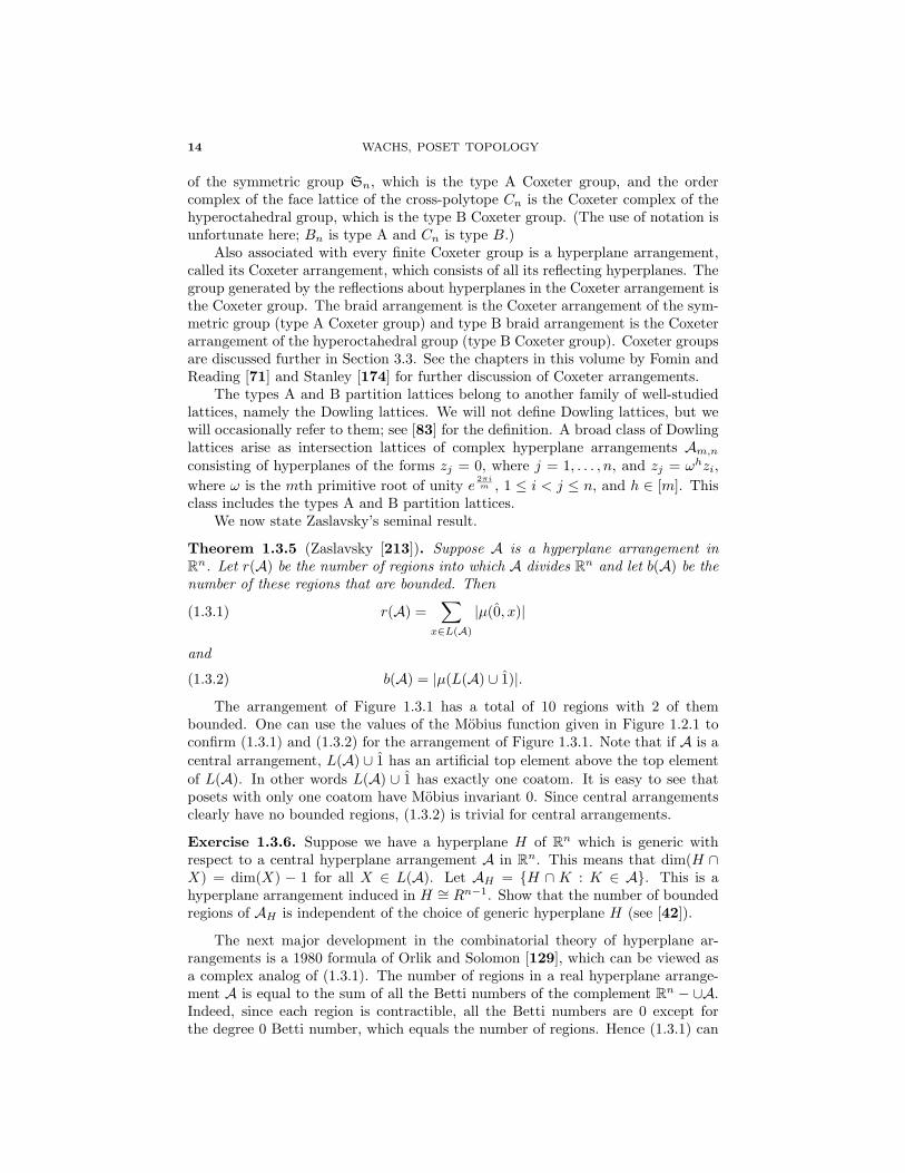
Theorem 1.3.5 (Zaslavsky [213]). Suppose A is a hyperplane arrangement inRn. Let r(A) be the number of regions into which A divides Rn and let b(A) be thenumber of these regions that are bounded. Then
(1.3.1) r(A) =∑
x∈L(A)
|µ(0, x)|
and
(1.3.2) b(A) = |µ(L(A) ∪ 1)|.The arrangement of Figure 1.3.1 has a total of 10 regions with 2 of them
bounded. One can use the values of the Mobius function given in Figure 1.2.1 toconfirm (1.3.1) and (1.3.2) for the arrangement of Figure 1.3.1. Note that if A is acentral arrangement, L(A) ∪ 1 has an artificial top element above the top elementof L(A). In other words L(A) ∪ 1 has exactly one coatom. It is easy to see thatposets with only one coatom have Mobius invariant 0. Since central arrangementsclearly have no bounded regions, (1.3.2) is trivial for central arrangements.
Exercise 1.3.6. Suppose we have a hyperplane H of Rn which is generic withrespect to a central hyperplane arrangement A in Rn. This means that dim(H ∩X) = dim(X) − 1 for all X ∈ L(A). Let AH = {H ∩ K : K ∈ A}. This is ahyperplane arrangement induced in H ∼= Rn−1. Show that the number of boundedregions of AH is independent of the choice of generic hyperplane H (see [42]).
The next major development in the combinatorial theory of hyperplane ar-rangements is a 1980 formula of Orlik and Solomon [129], which can be viewed asa complex analog of (1.3.1). The number of regions in a real hyperplane arrange-ment A is equal to the sum of all the Betti numbers of the complement Rn − ∪A.Indeed, since each region is contractible, all the Betti numbers are 0 except forthe degree 0 Betti number, which equals the number of regions. Hence (1.3.1) can

LECTURE 1. BASIC DEFINITIONS, RESULTS, AND EXAMPLES 15
be interpreted as a formula for the sum of the Betti numbers of the complementRn − ∪A. The analog for complex arrangements is given by following result.
Theorem 1.3.7 (Orlik and Solomon [129]). Let A be a hyperplane arrangementin Cn. The complement MA := Cn − ∪A has torsion-free integral cohomology andhas Betti numbers given by,
βi(MA) =∑
x ∈ L(A)
dimC(x) = n − i
|µ(0, x)|,
for all i.
There is a striking common generalization of the Zaslavsky formula (1.3.1) andthe Orlik-Solomon formula, obtained by Goresky and MacPherson in 1988, whichinvolves subspace arrangements. A real subspace arrangement is a finite collectionof (affine) subspaces in Rn. Real hyperplane arrangements and complex hyper-plane arrangements are both examples of real subspace arrangements. Indeed,hyperplanes in Cn can be viewed as codimension 2 subspaces of R2n. Again theintersection semilattice L(A) is defined to be the semilattice of nonempty intersec-tions of subspaces in the subspace arrangement A.
Theorem 1.3.8 (Goresky and MacPherson [80]). Let A be a subspace arrangementin Rn. The reduced integral cohomology of the complement MA := Rn−∪A is givenby the group isomorphism
Hi(MA; Z) ∼=⊕
x∈L(A)\{0}
Hn−dim x−2−i((0, x); Z),
for all i.
To see that the Goresky-MacPherson formula reduces to the Zaslavsky formulaand to the Orlik-Solomon formula, one needs to understand the homology of theintersection lattice of a central hyperplane arrangement. The intersection latticebelongs to a well-understood class of lattices called geometric lattices. A fundamen-tal result due to Folkman [70] states that the proper part of any geometric latticeL has vanishing reduced homology in every dimension except the top dimension(i.e. dimension equal to l(L)− 2). In fact, the homotopy type is that of a wedge ofspheres of top dimension. The intersection lattice of an affine hyperplane arrange-ment belongs to a more general class of lattices called geometric semilattices, whichwere introduced and studied by Wachs and Walker [203]. The proper part of ageometric semilattice also has the homotopy type of a wedge of spheres of top di-mension. Topology of geometric (semi)lattices is discussed further in Sections 3.2.3and 4.2.
Exercise 1.3.9. Use Folkman’s result to show that the Goresky-MacPherson for-mula reduces to both the Zaslavsky formula and the Orlik-Solomon formula.
The intersection lattice of a hyperplane arrangement determines more than theadditive group structure of the integral cohomology of the complement. Orlik andSolomon show that it determines the ring structure as well. Ziegler [216] showedthat, in general, for subspace arrangements the combinatorial data (intersectionlattice and dimension information) does not determine ring structure. Howeverin certain special cases the combinatorial data does determine the cohomology

16 WACHS, POSET TOPOLOGY
algebra, see [69], [212], [58]. In Section 5.4 we discuss some stronger versions ofthe Goresky-MacPherson formula, namely a homotopy version due to Ziegler andZivaljevic [220], and an equivariant version due to Sundaram and Welker [184].For further reading on hyperplane arrangements, see the chapter by Stanley inthis volume [174] and the text by Orlik and Terao [130]. Further information onsubspace arrangements can be found in Bjorner [28] and Ziegler [214].
1.4. Some connections with graphs, groups and lattices
In this section we briefly discuss some results and questions in which poset topologyplays a role. We start with a old conjecture of Karp in graph complexity theory. Analgorithm for deciding whether a graph with n nodes has a certain property checksthe entries of the graph’s adjacency matrix until a determination can be made. Agraph property is said to be evasive if the best algorithm needs to check all
(n2
)entries (in the worst case). Here are some examples of evasive graph properties:
• property of being connected• property of containing a perfect matching• property of having degree at most b for some fixed b.
A monotone graph property is a property of graphs that is isomorphism in-variant and closed under addition of edges or closed under removal of edges. Thegraph properties listed above are clearly monotone graph properties. We say thata graph property is trivial if every graph has the property or every graph lacks theproperty.
Conjecture 1.4.1 (Karp’s Evasiveness Conjecture). Every nontrivial monotonegraph property is evasive.
Kahn, Saks, and Sturtevant [106] proved the evasiveness conjecture for n aprime power by using topological techniques and group actions. Since determiningwhether a graph has a certain property is equivalent to determining whether thegraph lacks the property, one can require without loss of generality that a monotonegraph property be closed under removal of edges. Given such a monotone graphproperty, P, let ∆n
P be the simplicial complex whose vertex set is([n]2
)and whose
faces are the edge sets of graphs on node set [n] that have the property. Alter-natively, ∆n
P is the simplicial complex whose face poset is the poset of graphs onnode set [n] that have property P, ordered by edge set inclusion. Kahn, Saks, andSturtevant show that
• nonvanishing reduced simplicial homology of ∆nP implies P is evasive
• ∆nP has nonvanishing reduced simplicial homology when n is a prime
power, using a topological fixed point theorem.Although this connection between evasiveness and topology doesn’t really in-
volve posets directly, we mention it here because posets and simplicial complexescan be viewed as the same object, and as we will see in later in these lectures, thetools of poset topology are useful in the study of the topology of graph complexes.For other significant results on evasiveness and topology of graph complexes, seeeg., [55], [211], [73]. This topic is discussed in greater depth in Forman’s chapterof this volume [74]. Applications of graph complexes in knot theory and group the-ory are discussed in Section 5.2. There are also connections between the topologyof graph complexes and commutative algebra, which are explored in the work of
LECTURE 1. BASIC DEFINITIONS, RESULTS, AND EXAMPLES 17
Reiner and Roberts [138] and Dong [61]. A direct application of poset topology ina different complexity theory problem is discussed in Section 3.2.4.
Representability questions in lattice theory deal with whether an arbitrarylattice can be represented as a sublattice, subposet or interval in a given class oflattices. We briefly discuss three examples that have connections to poset topology.
A result of Pudlak and Tuma [134] states that every lattice is isomorphic to asublattice of some partition lattice Πn. This implies that every lattice can be repre-sented as the intersection lattice of a subspace arrangement embedded in the braidarrangement. There is another representability result that is much easier to prove;namely that every meet semilattice can be represented as the intersection semilat-tice of some subspace arrangement, see [214]. From either of these representabilityresults, we see that, in contrast to the situation with hyperplane arrangements,where the topology of the proper part of the intersection semilattice is rather spe-cial (a wedge of spheres), any topology is possible for the intersection semilatticeof a general subspace arrangement. Indeed, given any simplicial complex ∆, thereis a linear subspace arrangement A such that L(A) is homeomorphic to ∆; namelyA is the linear subspace arrangement whose intersection lattice L(A) is isomorphicto the face lattice L(∆).
An open representability question is whether every lattice can be representedas an interval in the lattice of subgroups of some group ordered by inclusion. Anapproach to obtaining a negative answer to this question, proposed by Shareshian[153], is to establish restrictions on the topology of intervals in the subgroup lattice.
Conjecture 1.4.2 (Shareshian [153]). Let G be a finite group. Then every openinterval in the lattice of subgroups of G has the homotopy type of a wedge of spheres.
This conjecture was shown to hold for solvable groups by Kratzer and Thevenaz[112] (see Theorem 3.1.13 which strengthens the Kratzer-Thevenaz result). Furtherdiscussion of connections between poset topology and group theory can be foundin Section 5.2
Our last example deals with the order dimension of a poset P , which is definedto be the smallest integer n such that P can be represented as an induced subposetof a product of n chains. Order dimension is an important and extensively studiedposet invariant, see [189]. Reiner and Welker give a lower bound on order dimensionof a lattice in terms of its homology.
Theorem 1.4.3 (Reiner and Welker [141]). Let L be a lattice and let d be thelargest dimension for which the reduced integral simplicial homology of the properpart of L is nonvanishing. Then the order dimension of L is at least d + 2.
1.5. Poset homology and cohomology
By (co)homology of a poset, we usually mean the reduced simplicial (co)homologyof its order complex. On rare occasions, we will deal with nonreduced simplicialhomology. Although it is presumed that the reader is familiar with simplicial ho-mology and cohomology, we review these concepts for posets in terms of chains ofthe poset. For each poset P and integer j, define the chain space
Cj(P ;k) := k-module freely generated by j-chains of P,
where k is a field or the ring of integers.

18 WACHS, POSET TOPOLOGY
The boundary map ∂j : Cj(P ;k) → Cj−1(P ;k) is defined by
∂j(x1 < · · · < xj+1) =j+1∑i=1
(−1)i (x1 < · · · < xi < · · · < xj+1),
where the · denotes deletion. We have that ∂j−1∂j = 0, which makes (Cj(P ;k), ∂j)an algebraic complex. Define the cycle space Zj(P ;k) := ker ∂j and the boundaryspace Bj(P ;k) := im∂j+1. Homology of the poset P in dimension j is defined by
Hj(P ;k) := Zj(P ;k)/Bj(P ;k).
The coboundary map δj : Cj(P ;k) → Cj+1(P ;k) is defined by
(1.5.1) 〈δj(α), β〉 = 〈α, ∂j+1(β)〉where α ∈ Cj(P ;k), β ∈ Cj+1(P ;k), and 〈·, ·〉 is the bilinear form on ⊕j≥−1Cj(P ;k)for which the chains of P form an orthonormal basis. This is equivalent to saying
δj(x1 < · · · < xj) =j+1∑i=1
(−1)i∑
x∈(xi−1,xi)
(x1 < · · · < xi−1 < x < xi < · · · < xj),
for all chains x1 < · · · < xj , where x0 is the bottom element of P and xj+1
is the top element of P . Define the cocycle space to be Zj(P ;k) := ker δj andthe coboundary space to be Bj(P ;k) := imδj−1. Cohomology of the poset P indimension j is defined to be
Hj(P ;k) := Zj(P ;k)/Bj(P ;k).
When k is a field, Hj(P ;k) and Hj(P ;k) are isomorphic vector spaces. Thejth (reduced) Betti number of P is given by
βj(P ) := dim Hj(P ; C),
which is the same as the rank of the free part of Hj(P ; Z).We will work primarily with homology over C and Z. For x < y in P , we write
Hj(x, y) for the complex homology of the open interval (x, y) of P , and βj(x, y) forthe jth Betti number of the open interval (x, y). When x = y, define Hj(x, y) tobe C and βj(x, y) to be 1 if j = −2, and to be 0 for all other j.
Many of the posets that arise have the homotopy type of a wedge of spheres.We review a basic fact pertaining to wedges of spheres and a partial converse.
Theorem 1.5.1. Suppose ∆ has the homotopy type of a wedge of spheres of variousdimensions, where ri is the number of spheres of dimension i. Then for each i =0, 1, . . . ,dim ∆,
(1.5.2) Hi(∆; Z) ∼= Hi(∆; Z) ∼= Zri .
Theorem 1.5.2. If ∆ is simply connected and has vanishing reduced integral ho-mology in all dimensions but dimension n, where homology is free of rank r, then∆ has the homotopy type of a wedge of r spheres of dimension n.
The first tool that we mention for computing homology of posets and simplicialcomplexes is a very efficient computer software package called “SimplicialHomol-ogy”, developed by Dumas, Heckenbach, Sauders, and Welker [63]. One can run itinteractively or download the source file at the web site:

LECTURE 1. BASIC DEFINITIONS, RESULTS, AND EXAMPLES 19
x1 xm
c
c
a
b
Figure 1.6.1. Top coboundary relations: δ(c′c′′)
http://www.cis.udel.edu/∼dumas/Homology,where a manual can also be found. This package has been responsible for manyof the more recent conjectures in the field. Its output was also part of the proofsof (at least) three results on integral homology appearing in the literature; see[154, 155, 200].
1.6. Top cohomology of the partition lattice
The top dimensional cohomology of a poset has a particularly simple description.For the sake of simplicity assume P is pure of length d. Let M(P ) be the set ofmaximal chains of P and let M′(P ) be the set of chains of length d − 1. Sinceker δd = Cd(P ;k), we have the following presentation of top cohomology as a quo-tient of Cd(P ;k):
Hd(P ;k) = 〈M(P ) | coboundary relations〉,where the coboundary relations have the form δd−1(c) for c ∈ M′(P ). Each chainc in M′(P ) is the concatenation c′c′′ of two unrefinable chains c′ and c′′. If c′ isnot empty, let a be the maximum element of c1, and if c′ is empty, let a be 0 of P .If c′′ is not empty, let b be the minimum element of c′′, and if c′′ is empty, let b be1 of P . Clearly, [a, b] is an interval of length 2 in P . Let {x1, . . . , xm} be the set ofelements in the open interval (a, b). We have
δd−1(c) = ±(c′x1c′′ + · · · + c′xmc′′).
Hence the cohomology relations can be associated with the intervals of length 2 inP . See Figure 1.6.1.
We demonstrate the use of intervals of length 2 by deriving a presentation forthe top cohomology of the proper part of the partition lattice Πn. There are twotypes of length 2 closed intervals in Πn; see Figure 1.6.2. In Type I intervals, thereare 2 pairs of blocks {A, B} and {C, D} which are separately merged resulting inblocks A ∪ B and C ∪ D. In Type II intervals, there are 3 blocks A, B, C, whichare merged into one block A∪B ∪C. Type I intervals have 4 elements and type IIintervals have 5 elements.
The two types of intervals induce two types of cohomology relations, TypeI and Type II cohomology relations on maximal chains. It is convenient to usebinary trees on leaf set [n] to describe these relations. A maximal chain of Πn is

20 WACHS, POSET TOPOLOGY
A∪B/C∪D
A∪B/C/D A/B/C∪D
A/B/C/ D
A∪B∪C
A∪B/C A/B∪C
A/B/C/ D
A∪C/B
Type I interval Type II interval
Figure 1.6.2.
3 5 1
2 4
Figure 1.6.3.
just a sequence of merges of pairs of blocks. The binary tree given in Figure 1.6.3corresponds to the sequence of merges:
(1) merge blocks {3} and {5}(2) merge blocks {2} and {4}(3) merge blocks {2, 4} and {1}.
This corresponds to the maximal chain
1/2/35/4 <· 1/24/35 <· 124/35
of Π5 The internal nodes of the tree represent the merges, and the leaf sets of theleft and right subtrees of the internal nodes are the blocks that are merged. Thesequence of merges follows the postorder traversal of the internal nodes, i.e. firsttraverse the left subtree in postorder, then the right subtree in postorder, then theroot.
Given a binary tree T on leaf set [n], let c(T ) be the maximal chain of Πn
obtained by the procedure described above. Although not all maximal chains canbe obtained in this way, it can be seen that every maximal chain is equal, modulothe cohomology relations of Type I, to ±c(T ) for some T . So the set
{c(T ) : T is a binary tree on leaf set [n]}
generates top cohomology Hn−3(Πn;k). The Type I cohomology relations inducethe following relations
(1.6.1) c(· · · (A ∧ B) · · · ) = (−1)|A||B| c(· · · (B ∧ A) · · · ),

LECTURE 1. BASIC DEFINITIONS, RESULTS, AND EXAMPLES 21
where X∧Y denotes the binary tree whose left subtree is X and whose right subtreeis Y , and |X| denotes the number of internal nodes of X. The Type II cohomologyrelations induce the following relations
c(· · · (A ∧ (B ∧ C)) · · · ) + (−1)|C|c(· · · ((A ∧ B) ∧ C) · · · )(1.6.2)
+ (−1)|A|B|c(· · · (B ∧ (A ∧ C)) · · · ) = 0.
Exercise 1.6.1. Show that the Type I cohomology relations yield (1.6.1) and theType II cohomology relations yield (1.6.2).
The relations (1.6.1) and (1.6.2) resemble the relations satisfied by the bracketoperation of a Lie algebra. The Type I relation (1.6.1) corresponds to the anticom-muting relation and the Type II relation (1.6.2) corresponds to the Jacobi relation.Indeed there is a well-known connection between the top homology of the partitionlattice and the free Lie algebra which involves representations of the symmetricgroup. In the next lecture, we discuss representation theory.
Theorem 1.6.2 (Stanley [167], Klyachko [108], Joyal [104]). The representationof the symmetric group Sn on Hn−3(Πn; C) is isomorphic to the representation ofSn on the multilinear component of the free Lie algebra over C on n generatorstensored with the sign representation.
This result follows from a formula of Stanley for the representation of the sym-metric group on homology of the partition lattice (Theorem 4.4.7) and an earliersimilar formula of Klyachko for the free Lie algebra. The first purely combinatorialproof was obtained by Barcelo [14]. The presentation of top cohomology discussedabove appeared in an alternative combinatorial proof of Wachs [197]. It also ap-peared in the proof of a superalgebra version of this result obtained by Hanlon andWachs [91]. A k-analog of the Lie superalgebra result was also obtained by Hanlonand Wachs [91]. A type B version (Example 1.3.4) was obtained by Bergeron [16]and a generalization to Dowling lattices was obtained by Gottlieb and Wachs [83].


LECTURE 2Group actions on posets
In this lecture we give a crash course on the representation theory of the sym-metric group and then discuss some representations on homology that are inducedby symmetric group actions on posets. For further details on the representationtheory of the symmetric group and symmetric functions, we refer the reader to thefollowing excellent standard references [76, 124, 149, 172].
There are various reasons that we are interested in understanding how a groupacts on the homology of a poset. One is that this can be a useful tool in computingthe homology of the poset. Another is that interesting representations often arise.We limit our discussion to the symmetric group, but point out there are ofteninteresting analogous results for other groups such as the hyperoctahedral group,wreath product groups, and the general linear group.
2.1. Group representations
We restrict our discussion to finite groups G and finite dimensional vector spacesover the field C. A finite dimensional vector space V over C is said to be a repre-sentation of G if there is a group homomorphism
φ : G → GL(V ).
For g ∈ G and v ∈ V , we write gv instead of φ(g)(v) and view V as a moduleover the ring CG (G-module for short). The dimension of the representation V isdefined to be the dimension of V as a vector space.
There are two particular representations of every group that are very important;the trivial representation and the regular representation. The trivial representation,denoted 1G, is the 1-dimensional representation V = C, where gz = z for all g ∈ Gand z ∈ C. The (left) regular representation is the G-module CG where G acts onitself by left multiplication, i.e., the action of g ∈ G on generator h ∈ G is gh.
We say that V1 and V2 are isomorphic representations of G and write V1∼=G V2,
if there is a vector space isomorphism ψ : V1 → V2 such that
ψ(gv) = gψ(v)
for all g ∈ G and v ∈ V1. In other words, V1 and V2 are isomorphic representationsof G means that they are isomorphic G-modules.
23

24 WACHS, POSET TOPOLOGY
The character of a G-module V is a function χV : G → C defined by
χV (g) = trace(φ(g)).
One basic fact of representation theory is that the character of a representationcompletely determines the representation. Another is that χV (g) depends only onthe conjugacy class of g.
A G-module V is said to be irreducible if its only submodules are the trivialsubmodule 0 and V itself. A basic result of representation theory is that the numberof irreducible representations of G is the same as the number of conjugacy classesof G. Another very important fact is that every G-module decomposes into a directsum of irreducible submodules,
V ∼=G V1 ⊕ · · · ⊕ Vm.
The decomposition is unique (up to order and up to isomorphism). Hence it makessense to talk about the multiplicity of an irreducible in a representation. We havethe following fundamental fact.
Theorem 2.1.1. The multiplicity of any irreducible representation of G in theregular representation of G is equal to the dimension of the irreducible.
There are two operations on representations that are quite useful. The first iscalled restriction. For H a subgroup of G and V a representation of G, the restric-tion of V to H, denoted V ↓G
H , is the representation of H obtained by restrictingφ to H. Thus the restriction has the same underlying vector space with a smallergroup action. The other operation, which is called induction, is a bit more compli-cated. For H a subgroup of G and V a representation of H, the induction of V toG is given by
V ↑GH := CG ⊗CH V,
where the tensor product A ⊗S B denotes the usual tensor product of an (R, S)-bimodule A and a left S-module B resulting in a left R-module. Now the underlyingvector space of the induction is larger than V .
Exercise 2.1.2. Show
dimV ↑GH=
|G||H| dimV.
Although restriction and induction are not inverse operations, they are relatedby a formula called Frobenius reciprocity. We will state an important special case,which is, in fact, equivalent to Frobenius reciprocity.
Theorem 2.1.3. Let U be an irreducible representation of H and let V be anirreducible representation of G, where H is a subgroup of G. Then the multiplicityof U in V ↓G
H is equal to the multiplicity of V in U ↑GH .
There are two types of tensor products of representations. Given a represen-tation U of G and a representation V of H, the (outer) tensor product U ⊗ Vis a representation of G × H defined by (g, h)(u, v) = (gu, hv). Given two repre-sentations U and V of G, the (inner) tensor product, also denoted U ⊗ V , is therepresentation of G defined by g(u, v) = (gu, gv).
In these lectures we will describe representations in any of the following ways:• giving the character• giving an isomorphic representation

LECTURE 2. GROUP ACTIONS ON POSETS 25
• giving the multiplicity of each irreducible• using operations such as restriction, induction and tensor product.
2.2. Representations of the symmetric group
In this section, we construct the irreducible representations of the symmetric groupSn, which are called Specht modules and are denoted by Sλ, where λ is a partitionof n. We also discuss skew shaped Specht modules.
Let λ be a partition of n, i.e., a weakly decreasing sequence of positive integersλ = (λ1 ≥ · · · ≥ λk) whose sum is n. We write λ � n (or |λ| = n) and say that thelength l(λ) is k. We will also write λ = 1m12m2 · · ·nmn , if λ has mi parts of size ifor each i. Each partition λ is identified with a Young (or Ferrers) diagram whoseith row has λi cells. For example, the partition (4, 2, 2, 1) � 9 is identified with theYoung diagram
A Young tableau of shape λ � n is a filling of the Young diagram correspondingto λ, with distinct positive integers in [n]. A Young tableau is said to be standardif the entries increase along each row and column. For example, the Young tableauon the left is not standard, while the one on the right is.
8 2 4 17 59 36
1 2 4 73 65 89
Let Tλ be the set of Young tableaux of shape λ and let Mλ be the complexvector space generated by elements of Tλ. The symmetric group Sn acts on Mλ bypermuting entries of the Young tableaux. That is, for transposition σ = (i, j) ∈ Sn,the tableau σT is obtained from T by switching entries i and j. For example,
(2, 3)
8 2 4 17 59 36
=
8 3 4 17 59 26
.
The representation that we have described is clearly the left regular representationof Sn. One can also let Sn act as the right regular representation on Mλ. That isfor transposition σ = (i, j) ∈ Sn and T ∈ Tλ, the tableau Tσ is obtained from Tby switching the contents of the ith and jth cell under some fixed ordering of thecells of λ.
We will say that two tableaux in Tλ are row-equivalent if they have the samesequence of row sets. For example, the tableaux
8 2 4 17 59 36
and
1 2 4 85 73 96

26 WACHS, POSET TOPOLOGY
are row-equivalent. Column-equivalent is defined similarly. For shape λ, the rowstabilizer Rλ is defined to be the subgroup
Rλ := {σ ∈ Sn : Tσ and T are row-equivalent for all T ∈ Tλ}.Similarly, the column stabilizer Cλ is defined to be the subgroup
Cλ := {σ ∈ Sn : Tσ and T are column-equivalent for all T ∈ Tλ}.We now give two characterizations of the Specht module Sλ; one as a subspace
of Mλ generated by certain signed sums of Young tableaux called polytabloids;and the other as a quotient of Mλ by certain relations called row relations andGarnir relations. We caution the reader that our notions of polytabloids and Garnirrelations are dual to the usual notions given in standard texts such as [149].
We begin with the submodule characterization. For each T ∈ Tλ, define thepolytabloid of shape λ,
eT :=∑
α∈Rλ
∑β∈Cλ
sgn(β) Tαβ.
For example if
T = 1 23
then eT =(
1 23
− 3 21
)+
(2 13
− 3 12
).
Since the left and right action of Sn on Tλ commute, we have
(2.2.1) πeT = eπT ,
for all T ∈ Tλ and π ∈ Sn. We can now define the Specht module Sλ to be thesubspace of Mλ given by
Sλ := 〈eT : T ∈ Tλ〉.It follows from (2.2.1) that Sλ is an Sn-submodule of Mλ (under the left action).
Theorem 2.2.1. The Specht modules Sλ for all λ � n form a complete set ofirreducible Sn-modules.
A polytabloid eT is said to be a standard polytabloid if T is a standard Youngtableau. We will see shortly that the standard polytabloids of shape λ form a basisfor the Specht module Sλ.
Now we give the quotient characterization. The row relations are defined forall T ∈ Tλ and σ ∈ Rλ by
(2.2.2) rσ(T ) := Tσ − T.
For all i, j such that 1 ≤ j ≤ λi, let Ci,j(λ) be the set of cells in columns jthrough λi of row i and in columns 1 through j of row i + 1. Let Gi,j(λ) be thesubgroup of Sn consisting of permutations σ that fix all entries of the cells thatare not in Ci,j(λ) under the right action of σ on tableaux of shape λ. The Garnirrelations are defined for all i, j such that 1 ≤ j ≤ λi and for all T ∈ Tλ by
(2.2.3) gi,j(T ) :=∑
σ∈Gi,j(λ)
Tσ.
For example if
T =
7 1 5 103 4 29 811 6
and (i, j) = (1, 2)

LECTURE 2. GROUP ACTIONS ON POSETS 27
then the entries 1, 5, 10, 3, 4 are permuted while the remaining entries are fixed. So
g1,2(T ) =
7 1 3 45 10 29 811 6
+
7 1 3 410 5 29 811 6
+
7 1 3 54 10 29 811 6
+
7 1 3 510 4 29 811 6
+ . . .
Again, since the left and right action of Sn on Tλ commute, we have
πrσ(T ) = rσ(πT )πgi,j(T ) = gi,j(πT ),
for all π ∈ Sn. Consequently, the subspace Uλ of Mλ generated by the rowrelations (2.2.2) and the Garnir relations (2.2.3) is an Sn-submodule of Mλ.
Theorem 2.2.2. For all λ � n,
Sλ ∼=SnMλ/Uλ.
Now we can view the Specht module Sλ as the module generated by tableauxof shape λ subject to the row and Garnir relations.
Exercise 2.2.3. Prove Theorem 2.2.2 by first showing that,(a) Uλ ⊆ ker ψ, where ψ : Mλ → Sλ is defined by ψ(T ) = eT ,(b) the standard polytabloids eT are linearly independent,(c) the standard tableaux span Mλ/Uλ.
We have the following consequence of Exercise 2.2.3.
Corollary 2.2.4. The standard polytabloids of shape λ form a basis for Sλ. Thestandard tableaux of shape λ form a basis for Mλ/Uλ. Consequently dimSλ is equalto the number of standard tableaux of shape λ.
There is a remarkable formula for the number of standard tableaux of a fixedshape λ.
Theorem 2.2.5 (Frame-Robinson-Thrall hook length formula). For all λ � n,
dimSλ =n!∏
x∈λ hx,
where the product is taken over all cells x in the Young diagram λ, and hx is thenumber of cells in the hook formed by x, which consists of x, the cells that are belowx in the same column, and the cells to the right of x in the same row.
One can generalize Specht modules to skew shapes. By removing a smallerskew diagram µ from the northwest corner of a skew diagram λ, one gets a skewdiagram denoted by λ/µ. For example if λ = (4, 3, 3) and µ = (2, 1) then
λ/µ = .
Skew Specht modules Sλ/µ are defined analogously to “straight” Specht modules.There is a submodule characterization and a quotient characterization. Theo-rem 2.2.2 and Corollary 2.2.4 hold in the skew setting. There is a classical combina-torial rule for decomposing Specht modules of skew shape into irreducible straightshape Specht modules called the Littlewood-Richardson rule, which we will notpresent here.

28 WACHS, POSET TOPOLOGY
Example 2.2.6. Some important classes of skew and straight Specht modules arelisted below.
λ/µ = ··Sλ/µ = regular representation.
λ = · · · Sλ = trivial representation
λ = ... Sλ = sign representation
where the sign representation is the 1-dimensional representation V = C whosecharacter is sgn(σ), that is σz = sgn(σ)z for all σ ∈ Sn and z ∈ C. We denotethe sign representation by sgnn or S(1n) and we denote the trivial representationby 1Sn
or S(n).
Exercise 2.2.7. For skew or straight shape λ/µ, let χλ/µ denote the character ofthe representation Sλ/µ, and for σ ∈ Sn, let f(σ) denote the number of fixed pointsof σ.
(a) Show χ(n−1,1)(σ) = f(σ) − 1 for all σ ∈ Sn.(b) Show χ(n,1)/(1)(σ) = f(σ) for all σ ∈ Sn.(c) Find the character of each of the representations in Example 2.2.6.
A skew hook is a connected skew diagram that does not contain the subdiagram(2, 2). Each cell of a skew hook, except for the southwestern most and northeasternmost end cells, has exactly two cells adjacent to it. Each of the end cells has onlyone cell adjacent to it. Let H be a skew hook with n cells. We label the cells of Hwith numbers 1 through n, starting at the southwestern end cell, moving throughthe adjacent cells, and ending at the northeastern end cell. For example, we havethe labeled skew hook
118 9 10765
1 2 3 4
.
If cell i + 1 is above cell i in H then we say that the skew hook H has a descent ati. Let des(H) denote the set of descents of H. For each subset S of [n− 1], there isexactly one skew hook with n cells and descent set S. For example, the skew hook
is the only skew hook with 11 cells and descent set {4, 5, 6, 7, 10}.
The Specht modules of skew hook shape are called Foulkes representations.Note that for any skew hook H with n cells, the set of standard tableaux of shapeH corresponds bijectively to the set of permutations in Sn with descent set des(H).(The descent set des(σ) of a permutation σ ∈ Sn is the set of all i ∈ [n − 1] such

LECTURE 2. GROUP ACTIONS ON POSETS 29
that σ(i) > σ(i + 1).) Indeed, by listing the entries of cells 1 through n, one getsa permutation with descent set des(H). Hence by Corollary 2.2.4 for skew shapes,the dimension of the Foulkes representation SH is the number of permutations inSn with descent set des(H).
A descent of a standard Young tableau is an entry i that is in a higher rowthan i + 1. By applying the Littlewood-Richardson rule mentioned above, one getsthe following decomposition of the Foulkes representation into irreducibles,
SH =⊕λ�n
cH,λSλ,(2.2.4)
where cH,λ is the number of standard Young tableaux of shape λ and descent setdes(H).
Exercise 2.2.8. Use (2.2.4) to show that the regular representation of Sn decom-poses into Foulkes representations as follows:
CSn∼=Sn
⊕H∈SHn
SH ,
where SHn is the set of skew hooks with n cells.
The induction product of an Sj-module U and an Sk-module V is the Sj+k-module
U • V := (U ⊗ V ) ↑Sj+k
Sj×Sk.
(We are viewing Sj ×Sk as the subgroup of Sj+k consisting of permutations thatstabilize the sets {1, 2 . . . , j} and {j + 1, j + 2, . . . , j + k}.)
Exercise 2.2.9. If a skew shape D consists of two shapes λ and µ, where λ and µhave no rows or columns in common, we say that D is the disjoint union of λ andµ. Show that SD = Sλ • Sµ if D is the disjoint union of λ and µ. For example
S = S • S .
Exercise 2.2.10. Let λ � n.
(a) Show that
Sλ ↓Sn
Sn−1∼=Sn−1
⊕µ
Sµ
summed over all Young diagrams µ obtained from λ by removing a cellfrom the end of one of the rows of λ. (We are viewing Sn−1 as thesubgroup of Sn consisting of permutations that fix n.) For example,
S ↓S8S7
∼=S7 S ⊕ S ⊕ S .
(b) Show that
Sλ ↑Sn+1Sn
= Sλ • S(1) ∼=Sn+1
⊕µ
Sµ

30 WACHS, POSET TOPOLOGY
summed over all Young diagrams µ obtained from λ by adding a cell tothe end of one of the rows of λ. For example,
S • S ∼=S8 S ⊕ S ⊕ S .
There is an important generalization of Exercise 2.2.10 (b) known as Pieri’srule.
Theorem 2.2.11 (Pieri’s rule). Let m, n ∈ Z+. If λ � n then
Sλ • S(m) ∼=Sm+n
⊕µ
Sµ,
summed over all partitions µ of m + n such that µ contains λ and the skew shapeµ/λ has at most one cell in each column. Similarly
Sλ • S(1m) ∼=Sm+n
⊕µ
Sµ,
summed over all partitions µ of m + n such that µ contains λ and the skew shapeµ/λ has at most one cell in each row.
The conjugate of a partition λ is the partition λ′ whose Young diagram is thetranspose of that of λ.
Theorem 2.2.12. For all partitions λ � n,
Sλ ⊗ sgnn∼=Sn Sλ′
,
where the tensor product is an inner tensor product. This also holds for skewdiagrams.
Exercise 2.2.13. Let V be a representation of Sn. Show that
(V ⊗ sgnn) ↑Sn+1Sn
∼=Sn+1 V ↑Sn+1Sn
⊗ sgnn+1,
and(V ⊗ sgnn) ↓Sn
Sn−1∼=Sn−1 V ↓Sn
Sn−1⊗ sgnn−1.
2.3. Group actions on poset (co)homology
Let G be a finite group. A G-simplicial complex is a simplicial complex togetherwith an action of G on its vertices that takes faces to faces. A G-poset is a posettogether with a G-action on its elements that preserves the partial order; i.e., x <y ⇒ gx < gy. So if P is a G-poset then its order complex ∆(P ) is a G-simplicialcomplex and if ∆ is a G-simplicial complex then its face poset P (∆) is a G-poset.
A G-space is a topological space on which G acts as a group of homeomorphisms.If ∆ is a G-simplicial complex then the geometric realization ‖∆‖ is a G-space underthe natural induced action of G.
Example 2.3.1. The subset lattice Bn is an Sn-poset. The action of a permutationσ ∈ Sn on a subset {a1, . . . , ak} is given by
σ{a1, . . . , ak} = {σ(a1), . . . , σ(ak)}.(2.3.1)

LECTURE 2. GROUP ACTIONS ON POSETS 31
Example 2.3.2. The partition lattice Πn is an Sn-poset. The action of a permu-tation σ ∈ Sn on a partition {B1, . . . , Bk} is given by
σ{B1, . . . , Bk} = {σB1, . . . , σBk},(2.3.2)
where σBi is defined in (2.3.1). The symmetric group is isomorphic to the groupgenerated by reflections about hyperplanes in the braid arrangement. The actiondescribed here is simply the action of the reflection group on intersections of hy-perplanes in the braid arrangement.
Example 2.3.3. The face lattice Cn of the n-cross-polytope (or the face lattice ofthe n-cube) is an Sn[Z2]-poset. The wreath product group Sn[Z2] is also knownas the hyperoctahedral group or the type B Coxeter group (see Section 2.4 for thedefinition of wreath product). It is the group generated by reflections about thehyperplanes in the type B braid arrangement.
By viewing the n-cross-polytope as the convex hull of the points ±ei, i =1, . . . , n, one obtains the action of Sn[Z2] on Cn. We describe this action in com-binatorial terms. The (k − 1)-dimensional faces of the cross-polytope are convexhulls of certain k element subsets of {±ei : i ∈ [n]}. These are the ones that don’tcontain both ei and −ei for any i. Thus the (k − 1)-faces can be identified withk-subsets T of [n]∪ {i : i ∈ [n]} such that {i, i} � T for all i. By ordering these setsby containment, one gets the face poset of the n-cross-polytope. For example, the4-subset {3, 5, 6, 8} is identified with the convex hull of the points e3,−e5, e6,−e8.The elements of Sn[Z2] are identified with permutations σ of [n] ∪ {i : i ∈ [n]}for which σ(i) = σ(i) for all i (where ¯a = a). Then the action of a permutationσ ∈ Sn[Z2] on a k-subset {a1, . . . , ak} of [n] ∪ {i : i ∈ [n]} is given by (2.3.1).
Example 2.3.4. The type B partition lattice ΠBn is also an Sn[Z2]-poset. Recall
from Example 1.3.4 that the type B partition lattice ΠBn is the intersection lattice of
the type B braid arrangement. Since this arrangement is invariant under reflectionabout any hyperplane in the arrangement, elements of the reflection group Sn[Z2]map intersections of hyperplanes to intersections of hyperplanes. This gives theaction of Sn[Z2] on ΠB
n . There is a combinatorial description of the action analogousto (2.3.2) (see e.g. [83]).
Example 2.3.5. The lattice of subspaces of an n-dimensional vector space over afinite field F is a GLn(F )-poset, where the general linear group GLn(F ) acts in theobvious way.
Example 2.3.6. The lattice of subgroups of a finite group G ordered by inclusionis a G-poset, where G acts by conjugation.
Example 2.3.7. The semilattice of p-subgroups of a group G ordered by inclusionis a G-poset, where G acts by conjugation.
Let P be a G-poset. Since g ∈ G takes j-chains to j-chains, g acts as a linearmap on Cj(P ; C). It is easy to see that
g∂(c) = ∂(gc) and gδ(c) = δ(gc).
Hence g acts as a linear map on Hj(P ; C) and on Hj(P ; C). This means thatwhenever P is a G-poset, Hj(P ; C) and Hj(P ; C) are G-modules. The bilinearform (1.5.1), induces a pairing between Hj(P ; C) and Hj(P ; C), which allows one

32 WACHS, POSET TOPOLOGY
to view them as dual G-modules. For G = Sn or G = Sn[Z2],
Hj(P, C) ∼=G Hj(P, C)
since dual Sn-modules (resp., dual Sn[Z2]-modules) are isomorphic.Given a G-simplicial complex ∆, the natural homeomorphism from ∆ to its
barycentric subdivision ∆(P (∆)) commutes with the G-action. Consequently, forall j ∈ Z
Hj(∆; C) ∼=G Hj(P (∆); C),
and
Hj(∆; C) ∼=G Hj(P (∆); C).
Exercise 2.3.8. The maximal chains of Bn correspond bijectively to tableaux ofshape 1n via the map
t1t2...tn
�→ ({t1} ⊂ {t1, t2} ⊂ · · · ⊂ {t1, . . . , tn−1}).
(a) Show that the Garnir relations map to the coboundary relations. Conse-quently, the representation of Sn on the top cohomology Hn−2(Bn; C) isthe sign representation.
(b) Show that the polytabloids map to cycles in top homology.
There is an equivariant version of the Euler-Poincare formula (Theorem 1.2.8),known as the Hopf-trace formula. It is convenient to state this formula in termsof virtual representations, which we define first. The representation group G(G) ofa group G is the free abelian group on the set of all isomorphism classes [V ] ofG-modules V modulo the subgroup generated by all [V ⊕W ]− [V ]− [W ]. Elementsof the representation group are called virtual representations. If V is an actualrepresentation, we denote the virtual representation [V ] by V . Note that two virtualrepresentations A − B and C − D, where A, B, C, D are actual representations ofG, are equal in the representation group if and only if A⊕D ∼=G B⊕C in the usualsense. We will write A − B ∼=G C − D.
Theorem 2.3.9 (Hopf trace formula). For any G-simplicial complex ∆,
dim ∆⊕i=−1
(−1)iCi(∆; C) ∼=G
dim ∆⊕i=−1
(−1)iHi(∆; C)
We will usually suppress the C from our notation Hi(P ; C) (resp., Hi(P ; C))and write Hi(P ) (resp., Hi(P )) instead when viewing (co)homology as a G-module.
2.4. Symmetric functions, plethysm, and wreath product modules
Symmetric functions provide a convenient way of describing and computing repre-sentations of the symmetric group. In this section we give the basics of symmetricfunction theory. Then we demonstrate its use in computing homology of an inter-esting example known as the matching complex.

LECTURE 2. GROUP ACTIONS ON POSETS 33
2.4.1. Symmetric functions
Let x = (x1, x2, . . . ) be an infinite sequence of indeterminates. A homogeneoussymmetric function of degree n is a formal power series f(x) ∈ Q[[x]] in which eachterm has degree n and f(xσ(1), xσ(2), . . . ) = f(x1, x2, . . . ) for all permutations σ ofZ+.
Let Λn denote the set of homogeneous symmetric functions of degree n andlet Λ =
⊕n≥0 Λn. Then Λ is a graded Q-algebra, since αf(x) + βg(x) ∈ Λn if
f(x), g(x) ∈ Λn and α, β ∈ Q; and f(x)g(x) ∈ Λm+n if f(x) ∈ Λm and g(x) ∈ Λn.There are several important bases for the vector space Λn. We mention just
two of them here; the basis of power sum symmetric functions and the basis ofSchur functions. These bases are indexed by partitions of n. For n ≥ 1, let
pn =∑i≥1
xni
and let p0 = 1. The power sum symmetric function indexed by λ = (λ1 ≥ λ2 ≥· · · ≥ λk) is defined by
pλ := pλ1pλ2 . . . pλk.
Given a Young diagram λ, a semistandard tableau of shape λ is a filling of λ withpositive integers so that the rows weakly increase and the columns strictly increase.Let SSλ be the set of semistandard tableaux of shape λ. Given a semistandardtableau T , define w(T ) := xm1
1 xm22 · · · , where for each i, mi is the number of times
i appears in T . Now define the Schur function indexed by λ to be
sλ :=∑
T∈SSλ
w(T ).
Skew shaped Schur functions sD are defined analogously for all skew diagrams D.While it is obvious that the power sum symmetric functions are symmetric
functions, it is not obvious that the Schur functions defined this way are.
Theorem 2.4.1. The sets {pλ : λ � n} and {sλ : λ � n} form bases for Λn.Moreover, {sλ : λ � n} is an integral basis, i.e., a basis for the Z-module Λn
Zof
homogeneous symmetric functions of degree n with integer coefficients.
The Schur function s(n) is known as the complete homogeneous symmetricfunction of degree n and is denoted by hn. The Schur function s(1n) is known asthe elementary symmetric function of degree n and is denoted by en. There is animportant involution ω : Λn → Λn defined by
ω(sλ) = sλ′ ,
where λ′ is the conjugate of λ. Clearly
ω(hn) = en.
For the power sum symmetric functions we have
ω(pλ) = (−1)|λ|−l(λ)pλ.(2.4.1)
Exercise 2.4.2. Prove ∑n≥0
hn =∏i≥1
(1 − xi)−1,

34 WACHS, POSET TOPOLOGY
and ∑n≥0
en =∏i≥1
(1 + xi),
where h0 = e0 = 1.
The Frobenius characteristic ch(V ) of a representation V of Sn is the symmetricfunction given by
ch(V ) :=∑µ�n
1zµ
χV (µ) pµ,
where zµ := 1m1m1!2m2m2! . . . nmnmn! for µ = 1m12m2 . . . nmn and χV (µ) is thecharacter χV (σ) for σ ∈ Sn of conjugacy type µ. Some basic facts on Frobeniuscharacteristic are compiled in the next result.
Theorem 2.4.3.(a) For all (skew or straight) shapes λ,
ch(Sλ) = sλ.
(b) For all representations V of Sn,
ω(chV ) = ch(V ⊗ sgnn).
(c) For all representations U, V of Sn,
ch(U ⊕ V ) = ch(U) + ch(V )
(d) For all representations U of Sm and V of Sn,
ch(U • V ) = ch(U) ch(V ).
The direct sum⊕
n≥0 G(Sn) of representation groups is a ring under the induc-tion product. It follows from Theorem 2.4.3 that the Frobenius characteristic mapis an isomorphism from the ring
⊕n≥0 G(Sn) to the ring of symmetric functions
over Z.
Definition 2.4.4. Let f ∈ Λ and let g be a formal power series with positiveinteger coefficients. Choose any ordering of the monomials of g, where a monomialappears in the ordering mi times if its coefficient is mi. For example, if g =3y1y
22 + 2y2y3 + . . . then the monomials can be arranged as
(y1y22 , y1y
22 , y1y
22 , y2y3, y2y3, . . . ).
Pad the sequence of monomials with zero’s if g has a finite number of terms. Definethe plethysm of f and g, denoted f [g], to be the formal power series obtained fromf by replacing the indeterminate xi with the ith monomial of g for each i. Sincef is a symmetric function, the chosen order of the monomials doesn’t matter. Forexample, if f =
∑n≥0 en =
∏i≥1(1 + xi) and g is as above then
f [g] = (1 + y1y22)(1 + y1y
22)(1 + y1y
22)(1 + y2y3)(1 + y2y3) · · · .
The following proposition is immediate.
Proposition 2.4.5. Suppose f, g ∈ Λ and h is a formal power series with positiveinteger coefficients. Then
• If f has positive integer coefficients then f [pn] = pn[f ] is obtained byreplacing each indeterminate xi of f by xn
i .

LECTURE 2. GROUP ACTIONS ON POSETS 35
• (af + bg)[h] = af [h] + bg[h], where a, b ∈ Q• fg[h] = f [h]g[h].
Note that if g ∈ Λ has positive integer coefficients then f [g] ∈ Λ. One canextend the definition of plethysm to all g ∈ Λ, by using Proposition 2.4.5 and thefact that the power sum symmetric functions form a basis for Λ. Hence plethysmis a binary operation on Λ, which is clearly associative, but not commutative. Notethat the plethystic identity is p1 = h1. We say that f, g ∈ Λ are plethystic inversesof each other, and write g = f [−1], if f [g] = g[f ] = h1.
2.4.2. Composition product and wreath product
Our purpose for introducing plethysm in these lectures is that plethysm encodes aproduct operation on symmetric group representations called composition product,which is described below. (This description is based on an exposition given in[178].)
Let G be a finite group. The wreath product of Sm and G, denoted by Sm[G],is defined to be the set of (m + 1)-tuples (g1, g2, . . . , gm; τ) such that gi ∈ G andτ ∈ Sm with multiplication given by
(g1, . . . , gm; τ)(h1, . . . , hm; γ) = (g1hτ−1(1), . . . , gmhτ−1(m); τγ).
The following proposition is immediate.
Proposition 2.4.6. The map (α1, α2, . . . , αm; τ) �→ τ is a homomorphism fromSm[Sn] onto Sm.
Definition 2.4.7. Let V be an Sm-module and W be a G-module. Then thewreath product of V with W , denoted V [W ], is the inner tensor product of twoSm[G]-modules:
V [W ] = W⊗m ⊗ V ,
where W⊗m is the vector space W⊗m with Sm[G] action given by
(α1, . . . , αm; τ)(w1 ⊗ · · · ⊗ wm) = α1wτ−1(1) ⊗ · · · ⊗ αmwτ−1(m)(2.4.2)
and V is the pullback of the representation of Sm on V to Sm[G] through thehomomorphism given in Proposition 2.4.6. That is, V is the representation ofSm[G] on V defined by
(α1, . . . , αm; τ)v = τv.
Given a finite set A = {a1 < a2 < · · · < an} of positive integers, let SA be theset of permutations of the set A. We shall view a permutation in SA as a word whoseletters come from A. For σ ∈ Sn, let σA denote the word aσ(1)aσ(2) · · · aσ(n). Weshall view an element of the Young subgroup Sk×Sn−k of Sn as the concatenationα � β of words α ∈ Sk and β ∈ S{k+1,...,n}. The wreath product Sm[Sn] isisomorphic to the normalizer of the Young subgroup Sn × · · · × Sn︸ ︷︷ ︸
m times
in Smn. The
isomorphism is given by
(α1, . . . , αm; τ) �→ αAτ(1)
τ(1) � · · · � αAτ(m)
τ(m) ,
where Ai = [in] \ [(i − 1)n].

36 WACHS, POSET TOPOLOGY
Define the composition product of an Sm-module V and an Sn-module W by
V ◦ W := V [W ] ↑Smn
Sm[Sn]
The following result relates plethysm to composition product.
Theorem 2.4.8. Let V be an Sm-module and W be an Sn-module. Then
ch(V ◦ W ) = chV [chW ].
Example 2.4.9. Given λ � n, let Π(λ) be the set of partitions of [n] whose blocksizes form the partition λ. In this example, we set λ = db, where d and b arepositive integers.
(a) The symmetric group Sbd acts on Π(db) as in Example 2.3.2, and this actioninduces a representation of Sbd on the complex vector space CΠ(db) generated byelements of Π(db). It is not difficult to see that the Sbd-module CΠ(db) is theinduction of the trivial representation of the stabilizer of the partition
π(db) := 1, . . . , d / d + 1, . . . , 2d / . . . / (b − 1)d + 1, . . . , bd
to Sbd. The stabilizer of π(db) is Sb[Sd] and the trivial representation of Sb[Sd]is S(b)[S(d)]. So CΠ(db) is the composition product S(b) ◦ S(d). By Theorem 2.4.8
ch CΠ(db) = hb[hd].
(b) The stabilizer Sb[Sd] of π(db) acts on the interval (π(db), 1) of Πbd. Thisinduces a representation of Sb[Sd] on the top homology Hb−3(π(db), 1) (recallHi(x, y) denotes complex homology of the open interval (x, y)). By observing thatthe interval (π(db), 1) is isomorphic to the poset Πb, one can see that
Hb−3(π(db), 1) ∼=Sb[Sd] Hb−3(Πb)[S(d)].
Next observe that⊕
x∈Π(db) Hb−3(x, 1) is the induction of Hb−3(π(db), 1) fromSb[Sd] to Sbd. So
⊕x∈Π(db) Hb−3(x, 1) is the composition product Hb−3(Πb)◦S(d).
By Theorem 2.4.8,
ch⊕
x∈Π(db)
Hb−3(x, 1) = ch Hb−3(π(db), 1) ↑Sbd
Sb[Sd]
= (ch Hb−3(Πb))[hd].
Theorem 2.4.8 is inadequate when λ is not of the form db. In [175, 199], more gen-eral results are given, which enable one to derive the following generating function,(2.4.3) ∑
λ∈Par(T,b)
(ch
⊕x∈Π(λ)
Hb−3(x, 1))
zλ1 · · · zλb= (ch Hb−3(Πb))
[ ∑i∈T
zihi
],
where T is any set of positive integers, Par(T, b) is the set of partitions of length b,all of whose parts are in T , the λi are the parts of λ, and the zi are (commuting)indeterminates.
2.4.3. The matching complex
In this subsection, we further demonstrate the power of symmetric function theoryand plethysm in computing homology. Our example is a well-studied simplicialcomplex known as the matching complex, which is defined to be the simplicialcomplex Mn whose vertices are the 2-element subsets of [n] and whose faces are

LECTURE 2. GROUP ACTIONS ON POSETS 37
collections of mutually disjoint 2-element subsets of [n]. Alternatively, Mn is thesimplicial complex of graphs on node set [n] whose degree is at most 2. Its faceposet is the proper part of the poset of partitions of [n] whose block sizes are atmost 2. It is not difficult to see that
ch Ck−1(Mn) = ek[h2]hn−2k.(2.4.4)
It follows from this and the Hopf trace formula (Theorem 2.3.9) that∑k≥−1
(−1)k−1chHk(Mn) =∑k≥0
(−1)kek[h2]hn−2k,
which implies by Exercise 2.4.2 that∑n≥0
∑k≥−1
(−1)k−1chHk(Mn) =∏i≤j
(1 − xixj)∏i≥1
(1 − xi)−1.
The right hand side can be decomposed into Schur functions by using the followingsymmetric function identity of Littlewood [121, p.238]:∏
i≤j
(1 − xixj)∏i≥1
(1 − xi)−1 =∑λ=λ′
(−1)|λ|−r(λ)
2 sλ,
where r(λ) is the rank of λ, i.e., the size of the main diagonal (or Durfee square)of the Young diagram for λ. From this we conclude that⊕
k≥−1
(−1)k−1Hk(Mn) ∼=Sn
⊕λ : λ � nλ = λ′
(−1)|λ|−r(λ)
2 Sλ.
With additional work involving long exact sequences of relative homology, Boucobtains the following beautiful refinement.
Theorem 2.4.10 (Bouc [47]). For all n ≥ 1 and k ∈ Z,
Hk−1(Mn) ∼=Sn
⊕λ : λ � nλ = λ′
r(λ) = |λ| − 2k
Sλ.(2.4.5)
From Bouc’s formula one obtains a formula for the Betti number in dimensionk − 1 as the number of standard Young tableaux of self-conjugate shape and rankn − 2k (which can be computed from the hook-length formula, Theorem 2.2.5).This result provides an excellent illustration of the use of representation theory inthe computation of Betti numbers.
We sketch a proof of Theorem 2.4.10 due to Dong and Wachs [62], whichinvolves a technique called discrete Hodge theory. Let ∆ be a G-simplicial complex.The combinatorial Laplacian Λk : Ck(∆) → Ck(∆) is defined by
Λk = δk−1∂k + ∂k+1δk.
A basic result of discrete Hodge theory is that
Hk(∆) ∼=G kerΛk.(2.4.6)
The key observation of [62] is that when one applies the Laplacian Λk−1 to anoriented simplex γ ∈ Ck−1(Mn), one gets
Λk−1(γ) = Tn · γ,

38 WACHS, POSET TOPOLOGY
where Tn =∑
1≤i<j≤n(i, j) ∈ CSn and (i, j) denotes a transposition. It is thenshown that Tn acts on the Specht module Sλ as multiplication by the scalar cλ
defined by
cλ =r∑
i=1
((αi + 1
2
)−
(βi + 1
2
)),
where r = r(λ), αi = λi − i, and βi = λ′i − i. That is, αi is the number of cells to
the right of and in the same row as the ith cell of the diagonal of λ and βi is thenumber of cells below and in the same column as the ith cell of the diagonal. Thearray (α1, . . . , αr | β1, . . . , βr) is known as Frobenius notation for λ. Note that λ isuniquely determined by its Frobenius notation.
Next we decompose Ck−1(Mn) into Specht modules by using (2.4.4) and an-other symmetric function identity of Littlewood, cf., [124, I 5 Ex. 9b], namely,∏
i≤j
(1 − xixj) =∑ν∈B
(−1)|ν|/2sν ,
where B is the set of all partitions of the form (α1 + 1, . . . , αr + 1 | α1, . . . , αr)for some r. This and Pieri’s rule (Theorem 2.2.11) yield the decomposition intoirreducibles:
Ck−1(Mn) ∼=⊕
λ∈An
akλSλ,
whereAn = {(α1, . . . , αr | β1, . . . , βr) � n : r ≥ 1, αi ≥ βi ∀ i ∈ [r]}
and akλ is a nonnegative integer. If λ is self-conjugate then
akλ =
{1 if r(λ) = n − 2k
0 otherwise.
Clearly for λ ∈ An, we have cλ = 0 if and only if λ is self-conjugate. It followsthat
ker Λp−1∼=
⊕λ : λ � nλ = λ′
akλ Sλ ∼=
⊕λ : λ � nλ = λ′
r(λ) = n − 2k
Sλ.
Theorem 2.4.10 now follows by discrete Hodge theory (2.4.6).There is a bipartite analog of the matching complex called the m × n chess-
board complex. This is the simplicial complex of subgraphs of the complete bi-partite graph on node sets of size m and n, whose nodes have degree at most 1.Alternatively, it is the simplicial complex of nonattacking rook placements on anm × n chessboard. Friedman and Hanlon [75] use discrete Hodge theory to obtaina chessboard complex analog of Bouc’s formula (2.4.5). (In fact the proof of (2.4.5)described above was patterned on the Friedman-Hanlon proof.) Not only can theBetti numbers be computed from this formula, but Shareshian and Wachs [155] usethe formula to compute torsion in the integral homology of the chessboard complex;see Theorem 5.5.5. So representation theory has proved to be a useful tool in com-puting torsion in integral homology as well as Betti numbers. Karaguezian, Reinerand Wachs [105] use formula (2.4.5) and its chessboard complex analog to derivea more general result of Reiner and Roberts [138], which computes the homologyof general bounded degree graph and bipartite graph complexes.

LECTURE 2. GROUP ACTIONS ON POSETS 39
The matching complex and chessboard complex have arisen in various areas ofmathematics, such as group theory (see Section 5.2), commutative algebra [138]and discrete geometry [221]. These complexes are discussed further in Lecture 5.See [200] for a survey article on the topology of matching complexes, chessboardcomplexes and general bounded degree graph complexes.


LECTURE 3Shellability and edge labelings
3.1. Shellable simplicial complexes
Shellability is a combinatorial property of simplicial and more general cell com-plexes, with strong topological and algebraic consequences. Shellability first ap-peared in the middle of the nineteenth century in Schlafli’s computation of theEuler characteristic of a convex polytope [150]. Schlafli made the assumption,without proof, that the boundary complex of a convex polytope is shellable. Thisassumption was eventually proved in 1970 by Brugesser and Mani [52] and wasused in McMullen’s proof [126] of the famous upper bound conjecture for convexpolytopes (the upper bound conjecture is stated in Section 4.1).
The original theory of shellability applied only to pure complexes. In the early1990’s, a nonpure simplicial complex arose in the complexity theory work of Bjorner,Lovasz and Yao [34] with topological properties somewhat similar to those of pureshellable complexes. This led Bjorner and Wachs [40, 41] to extend the theoryof shellability to nonpure complexes. The Goresky-MacPherson formula created aneed for such an extension, since, unlike for hyperplane arrangements, the inter-section semilattice of a subspace arrangement is not necessarily pure. As it turnedout, there were many other uses for nonpure shellability.
For each face F of a simplicial complex ∆, let 〈F 〉 denote the subcomplexgenerated by F , i.e., 〈F 〉 = {G : G ⊆ F}. A simplicial complex ∆ is said to beshellable if its facets can be arranged in linear order F1, F2, . . . , Ft in such a waythat the subcomplex
(⋃k−1i=1 〈Fi〉
)∩ 〈Fk〉 is pure and (dimFk − 1)-dimensional for
all k = 2, . . . , t. Such an ordering of facets is called a shelling. We emphasizethat we are not assuming purity; here shellability refers to what is commonly callednonpure shellability.
A shelling of the boundary complex of the 3-simplex is given in Figure 3.1.1.A pure nonshellable complex and a nonpure shellable complex are given in Fig-ure 3.1.2, where the shading indicates that the triangles are filled in.
41

42 WACHS, POSET TOPOLOGY
1 1 2 1 2
34
Figure 3.1.1. Shelling of the boundary of 3-simplex
Figure 3.1.2
Exercise 3.1.1. Verify that the third and fifth simplicial complexes below are notshellable, while the others are.
Theorem 3.1.2 (Brugesser and Mani [52]). The boundary complex of a convexpolytope is shellable.
A geometric construction called a line shelling is used to prove this result. SeeZiegler’s book [218] on polytopes for a description of this basic construction.
Shellability is not a topological property. By this we mean that shellability of acomplex is not determined by the topology of its geometric realization; a shellablesimplicial complex can be homeomorphic to a nonshellable simplicial complex. Infact, there exist nonshellable triangulations of the 3-ball and the 3-sphere; see[118],[218, Chapter 8], [219], [123].

LECTURE 3. SHELLABILITY AND EDGE LABELINGS 43
Shellability does have strong topological consequences, however, as is shown bythe following result. By a wedge ∨n
i=1Xi of n mutually disjoint connected topologicalspaces Xi, we mean the space obtained by selecting a base point for each Xi andthen identifying all the base points with each other.
Theorem 3.1.3 (Bjorner and Wachs [40]). A shellable simplicial complex has thehomotopy type of a wedge of spheres (in varying dimensions), where for each i, thenumber of i-spheres is the number of i-facets whose entire boundary is contained inthe union of the earlier facets. Such facets are usually called homology facets.
Proof idea. Let ∆ be a shellable simplicial complex. We first observe that anyshelling of ∆ can be rearranged to produce a shelling in which the homology facetscome last. So ∆ has a shelling F1, F2, . . . Fk in which F1, . . . , Fj are not homologyfacets and Fj+1, . . . , Fk are, where 1 ≤ j ≤ k. The basic idea of the proof is that aswe attach the first j facets, we construct a contractible simplicial complex at eachstep. The remaining homology facets attach as spheres since the entire boundaryof the facet is identified with a point. �Corollary 3.1.4. If ∆ is shellable then for all i,
(3.1.1) Hi(∆; Z) ∼= Hi(∆; Z) ∼= Zri ,
where ri is the number of homology i-facets of ∆.
The homology facets yield more than just the Betti numbers; they form a basisfor cohomology. We discuss the connection with cohomology further in the contextof lexicographic shellability in the next section.
There are certain operations on complexes and posets that preserve shellability.For a simplicial complex ∆ and F ∈ ∆, define the link to be the subcomplex givenby
lk∆F := {G ∈ ∆ : G ∪ F ∈ ∆, G ∩ F = ∅}.Theorem 3.1.5 ([40]). The link of every face of a shellable complex is shellable.
Define the suspension of a simplicial complex ∆ to be
susp(∆) := ∆ ∗ {{a}, {b}},where ∗ denotes the join, and a = b are not vertices of ∆.
Theorem 3.1.6 ([40]). The join of two simplicial complexes is shellable if andonly if each complex is shellable. In particular, susp(∆) is shellable if and only if∆ is shellable.
Define the k-skeleton of a simplicial complex ∆ to be the subcomplex consistingof all faces of dimension k or less.
Theorem 3.1.7 ([41]). The k-skeleton of a shellable simplicial complex is shellablefor all k ≥ 0.
A simplicial complex ∆ is said to be r-connected (for r ≥ 0) if it is nonemptyand connected and its jth homotopy group πj(∆) is trivial for all j = 1, . . . , r.So 0-connected is the same as connected and 1-connected is the same as simplyconnected. A nonempty simplicial complex ∆ is said to be r-acyclic if its jthreduced integral homology group Hj(∆) is trivial for all j = 0, 1, . . . , r. We say thatX is (−1)-connected and (−1)-acyclic when ∆ is nonempty. It is also convenientto say that every simplicial complex is r-connected and r-acyclic for all r ≤ −2.

44 WACHS, POSET TOPOLOGY
It is a basic fact of homotopy theory that r-connected implies r-acyclic andthat the converse holds only for simply connected complexes. Another basic factis that a a simplicial complex is r-connected (r-acyclic) if and only if its (r + 1)-skeleton has the homotopy type (homology) of a wedge of (r + 1)-spheres. Thismakes shellability a useful tool in establishing r-connectivity and r-acyclicity.
Theorem 3.1.8. A simplicial complex is r-connected (and therefore r-acyclic) ifits (r + 1)-skeleton is pure shellable.
A poset P is said to be shellable if its order complex ∆(P ) is shellable. Thefollowing is an immediate consequence of Theorems 3.1.5 and 3.1.6.
Corollary 3.1.9.(a) A bounded poset P is shellable if and only if its proper part P is shellable.(b) Every (open or closed) interval of a shellable poset is shellable.(c) The join of two posets is shellable if and only if each of the posets is
shellable.
Theorem 3.1.10 (Bjorner and Wachs [41]). The product of bounded posets isshellable if and only if each of the posets is shellable.
Sometimes shellability has stronger topological consequences than homotopytype.
Theorem 3.1.11 (Danaraj and Klee [56]). Let ∆ be a pure shellable d-dimensionalsimplicial complex in which every codimension 1 face is contained in at most 2facets. Then ∆ is homeomorphic to a d-sphere or a d-ball. Moreover, ∆ is homeo-morphic to a d-sphere if and only if every codimension 1 face is contained in exactly2 facets.
Note that the condition on codimension 1 faces in the Danaraj and Klee theoremcan be expressed as follows: Closed length 2 intervals of L(∆) have at most 4elements. Pure posets in which every length 2 interval has exactly 4 elements aresaid to be thin. We have the following poset version of the Danaraj and Klee result.
Theorem 3.1.12 (Bjorner [23]). If P is pure, thin and shellable then P is isomor-phic to the face poset of a regular cell decomposition (a generalization of simplicialdecomposition; see [92]) of an l(P )-sphere.
Many natural classes of simplicial complexes and posets, which have arisen invarious fields of mathematics, have turned out to be shellable (pure or nonpure). Astriking illustration of the ubiquity of shellability is given by the following result.
Theorem 3.1.13 (Shareshian [151]). The lattice of subgroups of a finite group Gis shellable if and only if G is solvable.
The pure version of this result, which states that the lattice of subgroups ofa finite group G is pure shellable if and only if G is supersolvable, was proved byBjorner [21] in the late 70’s by introducing a technique called lexicographic shella-bility. Shareshian uses a general (nonpure) version of lexicographic shellability morerecently introduced by Bjorner and Wachs [40]. We discuss lexicographic shella-bility in the remaining sections of this lecture. Further discussion of connectionsbetween group theory and poset topology can be found in Section 5.2.
We end this section with two interesting conjectures. A pure simplicial complex∆ is said to be extendably shellable if every partial shelling of ∆ extends to a shelling

LECTURE 3. SHELLABILITY AND EDGE LABELINGS 45
of ∆. Tverberg (see [56]) conjectured that the boundary complex of every polytopeis extendably shellable. The conjecture was settled in the negative by Ziegler [219]who showed that there are simple and simplicial polytopes whose boundary complexis not extendably shellable. The conjecture is, however, true for the simplex sinceevery ordering of the facets of the boundary complex is a shelling. Hence thek = d − 1 case of the following conjecture holds.
Conjecture 3.1.14 (Simon [160]). For all k ≤ d, the k-skeleton of the d-simplexis extendably shellable.
Simon’s conjecture was shown to be true for k ≤ 2 by Bjorner and Eriksson[31], who extended the conjecture to all matroid complexes. Recently Hall [84]showed that the boundary complex of the 12-dimensional cross-polytope is a coun-terexample to the extended conjecture of Bjorner and Eriksson.
A simplicial complex ∆ is said to be minimally nonshellable (called an ob-struction to shellability in [198]) if ∆ is not shellable, but every proper inducedsubcomplex of ∆ is shellable. For example, the complex consisting of two disjoint1-simplexes is a minimally nonshellable complex (see Exercise 3.1.1). Billera andMyers [20] showed that this is the only minimally nonshellable order complex. Itis also the only 1-dimensional minimally nonshellable simplicial complex. It wasshown by Wachs [198] that the number of vertices in any 2-dimensional minimallynonshellable simplicial complex is either 5, 6 or 7; hence there are only finitely manysuch complexes.
Conjecture 3.1.15 (Wachs). There are only finitely many d-dimensional mini-mally nonshellable simplicial complexes (obstructions to shellability) for each d.
3.2. Lexicographic shellability
In the early 1970’s, Stanley [163, 164] introduced a technique for showing thatthe Mobius function of rank-selected subposets of certain posets alternates in sign.This technique involved labeling the edges of the Hasse diagram of the poset ina certain way. Stanley conjectured that the posets that he was considering wereCohen-Macaulay, a topological (and algebraic) property of simplicial complexesimplied by shellability (cf., Section 4.1). Bjorner [21] proved this conjecture byfinding a condition on edge labelings which implies shellability of the poset. Fromthis emerged the theory of lexicographic shellability, which was further developedin a series of papers by Bjorner and Wachs, first in the pure case [37, 38] and laterin the general (nonpure) case [40, 41].
There are two basic versions of lexicographic shellability, EL-shellability andCL-shellability. In this section we begin with the simpler but less powerful version,EL-shellability, and discuss some of its consequences.
An edge labeling of a bounded poset P is a map λ : E(P ) → Λ, where E(P ) isthe set of edges of the Hasse diagram of P , i.e., the covering relations x <· y of P ,and Λ is some poset (usually the integers Z with its natural total order relation).Given an edge labeling λ : E(P ) → Λ, one can associate a word
λ(c) = λ(0, x1)λ(x1, x2) · · ·λ(xt, 1)
with each maximal chain c = (0 <· x1 <· · · · <· xt <· 1). We say that c is increasingif the associated word λ(c) is strictly increasing. That is, c is increasing if
λ(0, x1) < λ(x1, x2) < · · · < λ(xt, 1).

46 WACHS, POSET TOPOLOGY
1
2
3
3 1
2
3
23
12
11
2
Figure 3.2.1. EL-labeling
We say that c is decreasing if the associated word λ(c) is weakly increasing. We canorder the maximal chains lexicographically by using the lexicographic order on thecorresponding words. Any edge labeling λ of P restricts to an edge labeling of anyclosed interval [x, y] of P . So we may refer to increasing and decreasing maximalchains of [x, y], and lexicographic order of maximal chains of [x, y].
Definition 3.2.1. Let P be a bounded poset. An edge-lexicographical labeling (EL-labeling, for short) of P is an edge labeling such that in each closed interval [x, y]of P , there is a unique increasing maximal chain, which lexicographically precedesall other maximal chains of [x, y].
An example of an EL-labeling of a poset is given in Figure 3.2.1. The leftmostchain, which has associated word 123, is the only increasing maximal chain of theinterval [0, 1]. It is also lexicographically less than all other maximal chains. Oneneeds to check each interval to verify that the labeling is indeed an EL-labeling.
A bounded poset that admits an EL-labeling is said to be edge-lexicographicshellable (EL-shellable, for short). The following theorem justifies the name.
Theorem 3.2.2 (Bjorner [21], Bjorner and Wachs [40]). Suppose P is a boundedposet with an EL-labeling. Then the lexicographic order of the maximal chains ofP is a shelling of ∆(P ). Moreover, the corresponding order of the maximal chainsof P is a shelling of ∆(P ).
Exercise 3.2.3. Prove Theorem 3.2.2.
It is for nonbounded posets that shellability has interesting topological conse-quences since the order complex of a bounded poset is a just a cone.
Theorem 3.2.4 (Bjorner and Wachs [40]). Suppose P is a poset for which Padmits an EL-labeling. Then P has the homotopy type of a wedge of spheres, wherethe number of i-spheres is the number of decreasing maximal (i + 2)-chains of P .The decreasing maximal (i + 2)-chains, with 0 and 1 removed, form a basis forcohomology Hi(P ; Z).
The first part of Theorem 3.2.4 is a consequence of Theorems 3.1.3 and 3.2.2.Indeed, the proper parts of the decreasing chains are the homology facets of theshelling of ∆(P ) induced by the lexicographic order of maximal chains of P . To es-tablish the second part, one needs only show that the proper parts of the decreasingchains span cohomology. This is proved by showing that the cohomology relationsenable one to express a maximal chain with an ascent as the negative of a sum

LECTURE 3. SHELLABILITY AND EDGE LABELINGS 47
ascent descents
lexicogrpahicallylarger
Figure 3.2.2. Straightening step
of lexicographically larger maximal chains. This provides a step in a “straighten-ing” algorithm for expressing maximum chains as linear combinations of decreasingmaximum chains. See Figure 3.2.2.
Remark 3.2.5. In Bjorner’s original version of EL-shellability, the unique increas-ing maximal chain was required to be weakly increasing and the decreasing chainswere required to be strictly decreasing. The two versions have the same topologicaland algebraic consequences, but it is unknown whether they are equivalent.
Example 3.2.6. In the EL-labeling given in Figure 3.2.1, the two rightmost maxi-mal chains are the only decreasing maximal chains. One has length 3 and the otherhas length 2. It follows form Theorem 3.2.4 that the order complex of the properpart of the poset has the homotopy type of a wedge of a 1-sphere and a 0-sphere.This is consistent with the fact that the order complex of the proper part of theposet consists of the barycentric subdivision of the boundary of a 2-simplex and anisolated point.
3.2.1. The Boolean algebra Bn.
There is a very natural EL-labeling of the Boolean algebra Bn; simply label thecovering relation A1 ⊂· A2 with the unique element in the singleton set A2 − A1.The maximal chains correspond to the permutations in Sn. It is easy to see thateach interval has a unique increasing chain that is lexicographically first. There isonly one decreasing chain which is consistent with the fact that ∆(Bn) is a sphere.See Figure 3.2.3.
For each k ≤ n, define the truncated Boolean algebra Bkn to be the subposet of
Bn given byBk
n = {A ⊆ [n] : |A| ≥ k}.Define an edge labeling λ of Bk
n ∪ {0} as follows:
λ(A1, A2) =
{max A2 if A1 = 0 and |A2| = k
a if A2 − A1 = {a}.
It is easy to check that this is an EL-labeling. The decreasing chains correspond topermutations with descent set {k, k +1, . . . , n− 1}. Hence dim Hn−k−1(Bk
n) equalsthe number of permutations in Sn with descent set {k, . . . , n−1}, which equals thenumber of standard Young tableaux of hook shape k1n−k. An equivariant version of
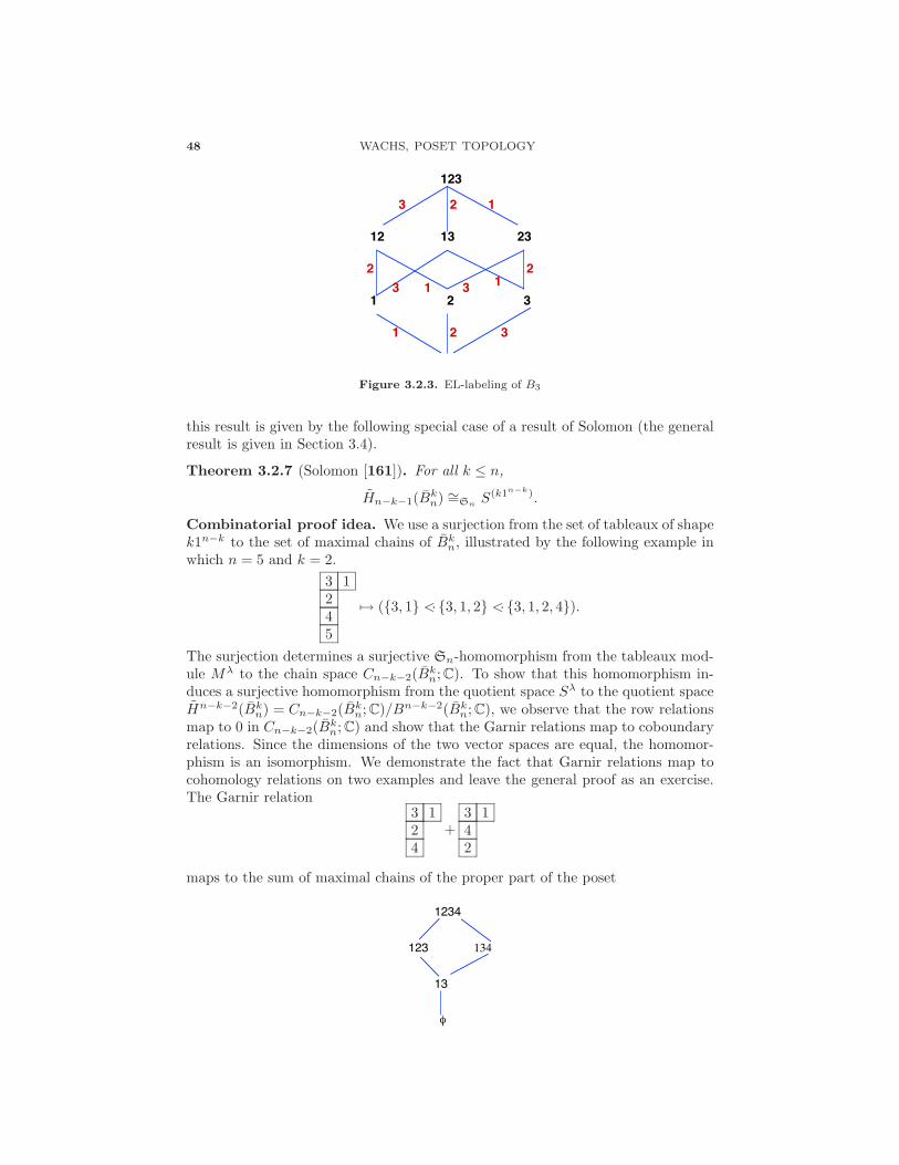
48 WACHS, POSET TOPOLOGY
12 13 23
1 2 3
123
1 2 3
1
2
1
2
3 3
3
1
2
Figure 3.2.3. EL-labeling of B3
this result is given by the following special case of a result of Solomon (the generalresult is given in Section 3.4).
Theorem 3.2.7 (Solomon [161]). For all k ≤ n,
Hn−k−1(Bkn) ∼=Sn
S(k1n−k).
Combinatorial proof idea. We use a surjection from the set of tableaux of shapek1n−k to the set of maximal chains of Bk
n, illustrated by the following example inwhich n = 5 and k = 2.
3 1245
�→ ({3, 1} <· {3, 1, 2} <· {3, 1, 2, 4}).
The surjection determines a surjective Sn-homomorphism from the tableaux mod-ule Mλ to the chain space Cn−k−2(Bk
n; C). To show that this homomorphism in-duces a surjective homomorphism from the quotient space Sλ to the quotient spaceHn−k−2(Bk
n) = Cn−k−2(Bkn; C)/Bn−k−2(Bk
n; C), we observe that the row relationsmap to 0 in Cn−k−2(Bk
n; C) and show that the Garnir relations map to coboundaryrelations. Since the dimensions of the two vector spaces are equal, the homomor-phism is an isomorphism. We demonstrate the fact that Garnir relations map tocohomology relations on two examples and leave the general proof as an exercise.The Garnir relation
3 124
+3 142
maps to the sum of maximal chains of the proper part of the poset
1234
123
13
φ
134

LECTURE 3. SHELLABILITY AND EDGE LABELINGS 49
The Garnir relation3 124
+2 134
+2 314
maps to the sum of maximal chains of the proper part of the poset
φ
13 12 23
123
1234
�
3.2.2. The partition lattice Πn.
We give two different EL-labelings of the partition lattice. The first one, due toGessel, appears in [21], and the second one is due to Wachs [196]. If x <· y in Πn
then y is obtained from x by merging two blocks, say B1 and B2. For the first edgelabeling λ1, let
λ1(x, y) = max{minB1,minB2}and for the second edge labeling λ2, let
λ2(x, y) = maxB1 ∪ B2.
The increasing chain from 0 to 1 is the same for both labelings; it consists ofpartitions with only one nonsingleton block. More precisely, the chain is given by
0 <· {1, 2} <· {1, 2, 3} <· · · · <· 1,
where we have written only the nonsingleton block of each partition in the chain.We leave it as an exercise to show that these labelings are EL-labelings of thepartition lattice.
The decreasing maximal chains for λ1 and λ2 are not the same. We describethose for λ2 first. They also consist of partitions with only one nonsingleton blockand are of the form
cσ := (0 <· {σ(n), σ(n − 1)} <· {σ(n), σ(n − 1), σ(n − 2)} <· · · ·<· {σ(n), σ(n − 1), σ(n − 2), . . . , σ(1)} = 1),
where σ ∈ Sn and σ(n) = n. We conclude that the homotopy type of Πn is givenby
(3.2.1) Πn �∨
(n−1)!
Sn−3
and that the chains cσ, where σ ∈ Sn and σ(n) = n, form a basis for Hn−3(Πn, Z).From this basis one can immediately see that
(3.2.2) Hn−3(Πn) ↓Sn
Sn−1∼=Sn−1 Hn−3(Πn) ↓Sn
Sn−1∼=Sn−1 CSn−1,
a result obtained by Stanley [167] as a consequence of his formula for the fullrepresentation of Sn on Hn−3(Πn) (Theorem 4.4.7).

50 WACHS, POSET TOPOLOGY
3124
3 / 1 2 43 1 / 2 4
3 1 2 / 4
3 / 1 / 2 4 3 / 1 2 / 4 3 1 / 2 / 4
3 / 1 / 2 / 4
Figure 3.2.4. Π3124
Next we describe a nice basis for homology of Πn that is dual to the decreasingchain basis for λ2. To split a permutation σ ∈ Sn at positions j1 < j2 < · · · < jk
in [n − 1] is to form the partition
σ(1), σ(2), . . . , σ(j1) / σ(j1+1), σ(j1+2), . . . , σ(j2) / . . . / σ(jk+1), σ(jk+2), . . . , σ(n)
of [n]. For each σ ∈ Sn, let Πσ be the induced subposet of the partition latticeΠn consisting of partitions obtained by splitting the permutation σ at any set ofpositions in [n − 1] . The subposet Π3124 of Π4 is shown in Figure 3.2.4. Eachposet Πσ is isomorphic to the subset lattice Bn−1. Therefore ∆(Πσ) is an (n − 3)-sphere embedded in ∆(Πn), and hence it determines a fundamental cycle ρσ ∈Hn−3(Πn; Z).
Theorem 3.2.8 (Wachs [196]). The set {ρσ : σ ∈ Sn, σ(n) = n} forms a basisfor Hn−3(Πn; Z) dual to the decreasing chain basis {cσ : σ ∈ Sn, σ(n) = n} forcohomology. Call the homology basis, the splitting basis.
Now we describe the decreasing chain basis for cohomology for the EL-labelingλ1 and its dual basis for homology. Given any rooted nonplanar (i.e. children of anode are unordered) tree T on node set [n], by removing any set of edges of T , oneforms a partition of [n] whose blocks are the node sets of the connected componentsof the resulting graph. Let ΠT be the induced subposet of the partition lattice Πn
consisting of partitions obtained by removing edges of T ; see Figure 3.2.5. (If T isa linear tree then ΠT is the same as Πσ, where σ is the permutation obtained byreading the nodes of the tree from the root down.) Each poset ΠT is isomorphicto the subset lattice Bn−1. We let ρT be the fundamental cycle of the sphericalcomplex ∆(ΠT ). Let T be an increasing tree on node set [n], i.e., a rooted nonplanartree on node set [n] in which each node i is greater than its parent p(i). We formthe chain cT in ΠT , from top down, by removing the edges {i, p(i)}, one at a time,in increasing order of i. For the increasing tree T in Figure 3.2.5,
cT = (1/2/3/4 <· 3/24/1 <· 324/1 <· 1234).
We claim that the cT , where T is an increasing tree on node set [n], are the de-creasing chains of λ1.

LECTURE 3. SHELLABILITY AND EDGE LABELINGS 51
1
2
3 4
1234
3 / 124 123 / 4 324 / 1
3 / 4 / 12 3 / 24 / 1 32 / 4 / 1
1 / 2 / 3 / 4
Figure 3.2.5. T and ΠT
Theorem 3.2.9. Let Tn be the set of increasing trees on node set [n]. The set{ρT : T ∈ Tn} forms a basis for Hn−3(Πn; Z) dual to the decreasing chain basis{cT : T ∈ Tn} for cohomology. Call the homology basis, the tree splitting basis.
Exercise 3.2.10.(a) Show λ1 is an EL-labeling whose decreasing maximal chains are of the
form cT , where T is an increasing tree.(b) Prove Theorem 3.2.9(c) Show λ2 is an EL-labeling whose decreasing maximal chains are of the
form cσ, where σ ∈ Sn is such that σ(n) = n.(d) Prove Theorem 3.2.8.
Both of the EL-labelings and their corresponding bases are special cases of moregeneral constructions. The first EL-labeling λ1 and its bases are specializations ofconstructions for geometric lattices due to Bjorner [21, 22]; this is discussed inthe next section. The second EL-labeling λ2 generalizes to all Dowling lattices;see the next exercise. A geometric interpretation of the splitting basis, in whichthe fundamental cycles correspond to bounded regions in an affine slice of the realbraid arrangement, is given by Bjorner and Wachs [42]. This leads to analogs of thesplitting basis for intersection lattices of other Coxeter arrangements, in particularthe type B partition lattice ΠB
n . An analog of the splitting basis for all Dowlinglattices is given by Gottlieb and Wachs [83].
Exercise 3.2.11 (Gottlieb [81, Section 7.3]).(a) Find an EL-labeling of the type B partition lattice ΠB
n analogous to theEL-labeling λ2 of Πn.
(b) Describe the decreasing chains in terms of signed permutations in Sn[Z2]whose right-to-left maxima are positive, where for i = 1, 2, . . . n, we saythat σ(i) is a right-to-left maxima of σ if |σ(i)| > |σ(j)| for all j = i . . . n.
(c) Show that the number of decreasing chains is (2n−1)!! := 1 ·3 · · · (2n−1),thereby recovering the well-known fact that ΠB
n has the homotopy typeof a wedge of (2n − 1)!!-spheres of dimension n − 2.
A partition π ∈ Πn is said to be noncrossing if for all a < b < c < d, whenevera, c are in a block B of π and b, d are in a block B′ of π then B = B′. Let NCn bethe induced subposet of Πn consisting of noncrossing partitions. This poset, knownas the noncrossing partition lattice, was first introduced by Kreweras [113] who

52 WACHS, POSET TOPOLOGY
showed that it is a graded lattice with Mobius invariant equal to the signed Catalannumber (−1)n−1 1
n
(2n−2n−1
). It has since undergone extensive study due to its many
fascinating properties and its connections to various diverse fields of mathematicssuch as combinatorics, discrete geometry, mathematical biology, geometric grouptheory, low dimensional topology, and free probability; see the survey papers ofSimion [159] and McCammond [125].
Bjorner and Edelman showed that NCn is EL-shellable (see Exercise 3.2.12).Reiner [137] introduced an analog of the noncrossing partition lattice for the typeB Coxeter group, and established many of the same properties held by NCn, includ-ing EL-shellability. A generalization of the types A and B noncrossing partitionlattices to all finite Coxeter groups was recently introduced in the geometric grouptheory /low dimensional topology work of Bessis [17] and Brady and Watt [49].This generalization is discussed in Section 3.3. The Mobius function for the typeD noncrossing partition lattice was computed by Athanasiadis and Reiner and thequestion of EL-shellability was raised [7]. The general Coxeter group noncross-ing partition lattices were subsequently shown to be EL-shellable by Athanasiadis,Brady and Watt [6].
Exercise 3.2.12 (Bjorner and Edelman, cf. [21]).(a) Show that the restriction to NCn of one of the EL-labelings of Πn described
above is an EL-labeling.(b) Describe the decreasing chains for the EL-labeling and show that their
number is the Catalan number 1n
(2n−2n−1
).
Exercise 3.2.13 (Stanley [171]). Define an edge labeling for NCn by
λ(x, y) = max{i ∈ B1 : i < minB2},where B1 and B2 are the blocks of x that are merged to obtain y and minB1 <minB2.
(a) Show that λ is an EL-labeling of NCn.(b) Show that the decreasing chains correspond bijectively, via the labeling,
to the sequences of the form (a1 ≥ a2 ≥ · · · ≥ an−1) where an−i ∈ [i]for all i ∈ [n − 1]. Show that the number of such sequences is a Catalannumber.
This labeling is particularly interesting because the maximal chains correspondbijectively, via this labeling, to a well-studied class of sequences called parkingfunctions; see [171].
3.2.3. Geometric lattices
A geometric lattice is a lattice L that is semimodular (which means that for allx, y ∈ L, the join x ∨ y covers y whenever x covers the meet x ∧ y) and atomic(which means every element of L is the join of atoms). Some fundamental examplesare the subset lattice Bn, the subspace lattice Bn(q), the partition lattice Πn, thetype B partition lattice ΠB
n , and more generally, the intersection lattice L(A) of anycentral hyperplane arrangement. Geometric lattices are fundamental structures ofmatroid theory. It is easy to show that geometric lattices are pure.
We describe an edge labeling for geometric lattices, which comes from Stanley’searly work [164] on rank-selected Mobius invariants and was one of the main moti-vating examples for Bjorner’s original work [21] on EL-shellability. Fix an ordering

LECTURE 3. SHELLABILITY AND EDGE LABELINGS 53
a1, a2, . . . , ak of the atoms of the geometric lattice L. Then label each edge x <· y ofthe Hasse diagram with the smallest i for which x∨ ai = y. Note that if the atomsof the subset lattice Bn are ordered {1}, {2}, . . . , {n}, then the geometric latticeEL-labeling is precisely the labeling given in Section 3.2.1.
Exercise 3.2.14.(a) Show that the edge labeling for geometric lattices described above is an
EL-labeling.(b) Find an ordering of the atoms of Πn such that the induced geometric
lattice EL-labeling is equivalent to the EL-labeling λ1 of Section 3.2.2.(c) Is λ2 of Section 3.2.2 equivalent to a geometric lattice EL-labeling for
some ordering of the atoms?(d) Show that every semimodular lattice has an EL-labeling.
The decreasing chains of the geometric lattice EL-labeling have a very nicecharacterization, due to Bjorner [22], which is described in the language of matroidtheory. A set A of atoms in a geometric lattice L is said to be independent ifr(∨A) = |A|. A set of atoms that is minimally dependent (i.e., every proper subsetis independent) is called a circuit. An independent set of atoms that can be obtainedfrom a circuit by removing its smallest element (with respect to the fixed orderinga1, a2, . . . , ak of the atoms of L) is called a broken circuit. A maximal independentset of atoms is said to be an NBC base if contains no broken circuits. There is anatural bijection from the NBC bases of L to the decreasing chains of L. Indeed,given any NBC base A = {ai1 , . . . , air}, where 1 ≤ i1 < i2 < · · · < ir ≤ k, constructthe maximal chain
cA := (0 < air< air
∨ air−1 < · · · < air∨ air−1 ∨ · · · ∨ ai1 = 1).
It is not difficult to check that the label sequence of cA is (ir, ir−1, . . . , i1), whichis decreasing, and that the map A �→ cA is a bijection from the NBC bases of L tothe decreasing chains of L. We conclude that the set {cA : A is an NBC base of L}is a basis for top cohomology of L.
Bjorner [22] also constructs a basis for homology of L indexed by the NBCbases, which is dual to the cohomology basis described above. Any independentset of atoms in a geometric lattice generates (by taking joins) a Boolean algebraembedded in the geometric lattice. Given any independent set of atoms A, let LA
be the Boolean algebra generated by A and let ρA be the fundamental cycle of LA.
Theorem 3.2.15 (Bjorner [22]). Fix an ordering of the set of atoms of a geometriclattice L. The set
{ρA : A is an NBC base of L}is a basis for top homology of L, which is dual to the decreasing chain basis
{cA : A is an NBC base of L}for top cohomology.
Exercise 3.2.16. Prove Theorem 3.2.15.
Exercise 3.2.17. Show that the tree splitting basis for homology of the partitionlattice is an example of a Bjorner NBC basis.
For further reading on the homology of geometric lattices see Bjorner’s bookchapter [26].

54 WACHS, POSET TOPOLOGY
123456
12345/6 12356/412346/5
123/456
1234/5/6 1235/4/6 1236/4/5
123/4 /5 /6
Figure 3.2.6. Interval of Π6,3
3.2.4. The k-equal partition lattice
In this section we present the original example that motivated the Bjorner-Wachsextension of the theory of shellability from pure to nonpure complexes. This inter-esting example played a pivotal role in two other important developments, namelythe use of poset topology in complexity theory (Bjorner, Lovasz and Yao [34, 33])and the derivation of the equivariant version of the Goresky-MacPherson formula(Sundaram and Welker [184]).
The k-equal partition lattice Πn,k is the subposet of Πn consisting of partitionsthat have no blocks of size {2, 3, . . . , k − 1}. This lattice is not a geometric latticewhen k > 2. It’s not even pure; consider the interval of Π6,3 shown in Figure 3.2.6.
The k-equal partition lattice arose in the early 1990’s from the “k-equal prob-lem” in complexity theory: Given a sequence of n real numbers x1, . . . , xn, deter-mine whether or not some k of them are equal. Bjorner, Lovasz and Yao [34, 33]obtained the following lower bound on the complexity of the k-equal problem bystudying the topology of Πn,k,
max{n − 1, n log3
n
3k}.
This lower bound differs by a factor of only 16 from the best upper bound. The k-equal problem translates into a subspace arrangement problem; namely determinewhether or not the point (x1, . . . , xn) is in the complement of the real subspacearrangement An,k, called the k-equal arrangement, consisting of subspaces of theform
{(x1, . . . , xn) ∈ Rn : xi1 = xi2 = · · · = xik},
where 1 ≤ i1 < · · · < ik ≤ n. Bjorner and Lovasz [33] show that the sum of theBetti numbers of the complement of the k-equal arrangement gives a lower boundfor the depth of the best decision tree for the k-equal problem. They then use theGoresky-MacPherson formula (Theorem 1.3.8) to reduce the complexity problemto that of studying the topology of lower intervals in the intersection lattice of An,k,which is isomorphic to Πn,k.

LECTURE 3. SHELLABILITY AND EDGE LABELINGS 55
Bjorner and Welker [45] prove that all open intervals of Πn,k have the homotopytype of a wedge of spheres of varying dimensions. Since homotopy type of a wedge ofspheres (of top dimension) is the main topological consequence of pure shellability,this result led Bjorner and Wachs to consider shellability for nonpure complexes.
We now present the nonpure EL-labeling of Πn,k obtained in [40] . First linearlyorder the label set {1 < 2 < · · · < n < 1 < 2 < · · · < n}. Now label the edge π <· τas follows:
λ(π, τ) =
⎧⎪⎨⎪⎩
max B if a new block B is formed from singleton blocksa if a nonsingleton block is merged with a singleton {a}max B1 ∪ B2 if two nonsingletons B1 and B2 are merged.
Exercise 3.2.18. Show that λ is an EL-labeling of Πn,k.
We next describe the decreasing maximal chains. Given a hook shape Youngdiagram k1m, by the corner of the hook we mean the cell in the first row andfirst column, and by the leg of T we mean the first column of T minus the corner.We refer to a skew diagram as a k-broken skew hook diagram if it is the disjointunion of hooks H1, H2, . . . , Ht of the form k1m, where m is arbitrary. The tableauxin Figure 3.2.7 are reverse standard tableaux (i.e. column and row entries aredecreasing rather than increasing) of 3-broken skew hook shape. For each reversestandard tableau T of k-broken skew hook shape, with entries in [n], let π
Tbe the
partition in Πn,k whose nonsingleton blocks are B1, . . . , Bt, where Bi is the set ofentries of T in the hook Hi. For the tableaux in Figure 3.2.7,
πT
= 15, 14, 3, 9, 8, 5/10, 7, 1, 2/13, 11, 4, 12, 6
and
πT ′ = 15, 14, 3, 9, 8, 5/10, 7, 1/13, 11, 4, 12, 6/2.
Given a reverse standard tableau T of k-broken skew hook shape, we let a be thesmallest entry among all entries of T that are either in the leg of a hook or in thecorner of a hook that has no leg. In the former case we let T ′ be the standardtableau of k-broken skew hook shape obtained by removing a from T . In the lattercase we let T ′ be the standard tableau of k-broken skew hook shape obtained byremoving the entire hook (which is a row) containing a. In either case, we refer tothe tableau T ′ as the predecessor of T . In Figure 3.2.7, T ′ is the predecessor of T .For each reverse standard tableau T of k-broken skew hook shape, with n cells andentries in [n], let cT be the maximal chain of Πn,k such that
• πT∈ cT
• the upper segment cT ∩ [πT, 1] is the chain
πT
= B1/B2/ . . . /Bt < B1 ∪ B2/B3/ . . . /Bt < · · · < B1 ∪ · · · ∪ Bt = 1
• the lower segment cT ∩ [0, πT] is the chain
0 = πT0
< πT1
< · · · < πTn−t(k−1)
= πT,
where Ti is the predecessor of Ti+1.
For the tableau T of Figure 3.2.7, the maximal chain cT is given by

56 WACHS, POSET TOPOLOGY
T =
13 11 4126
10 7 12
15 14 3985
T ′ =
13 11 4126
10 7 115 14 3985
Figure 3.2.7.
1 > 15, 14, 3, 9, 8, 5, 10, 7, 1, 2/13, 11, 4, 12, 6> 15, 14, 3, 9, 8, 5/10, 7, 1, 2/13, 11, 4, 12, 6> 15, 14, 3, 9, 8, 5/10, 7, 1/13, 11, 4, 12, 6> 15, 14, 3, 9, 8/10, 7, 1/13, 11, 4, 12, 6> 15, 14, 3, 9, 8/10, 7, 1/13, 11, 4, 12> 15, 14, 3, 9/10, 7, 1/13, 11, 4, 12> 15, 14, 3/10, 7, 1/13, 11, 4, 12> 15, 14, 3/13, 11, 4, 12> 15, 14, 3/13, 11, 4> 15, 14, 3> 0
where only the nonsingleton blocks are shown.
Exercise 3.2.19.(a) [40] Show that the set of decreasing chains with respect to λ is the set
{cT : T is a reverse standard tableau of k-broken skew hook shape,with n cells and n in the corner of the leftmost hook}.
(b) [40] Show that the Betti numbers are given by
βn−3−t(k−2)(Πn,k) =∑
j1 + j2 + . . . + jt = nji ≥ k
(n − 1
j1 − 1, j2, . . . , jt
) t∏i=1
(ji − 1k − 1
)
where t ≥ 1, and
βi(Πn,k) = 0
if i is not of the form n − 3 − t(k − 2) for any t ≥ 0.(c) [182] Prove that
Hn−3−t(k−2)(Πn,k) ↓Sn
Sn−1∼=Sn−1
⊕D
SD

LECTURE 3. SHELLABILITY AND EDGE LABELINGS 57
summed over all k-broken skew hook diagrams D of size n in which thecorner of the leftmost hook is removed. This is equivalent to
Hn−3−t(k−2)(Πn,k) ↓Sn
Sn−1∼=
⊕j1 + j2 + . . . + jt = n
ji ≥ k
S1jt−k • S(k−1) •t−1∏i=1
S(k1ji−k),
where • and∏
denote induction product.
The decreasing chains given in Exercise 3.2.19(a) were also used by Sundaramand Wachs [182] to obtain a formula for the unrestricted representation of Sn
on Hn−3−t(k−2)(Πn,k), involving composition product of representations. In or-der to transfer the representation of the symmetric group on homology of the k-equal partition poset to representations of the symmetric group on the homologyof the complement MAn,k
:= Rn −∪An,k of the real k-equal arrangement An,k andthe complement MAC
n,k:= Cn − ∪AC
n,k of the complex k-equal arrangement AC
n,k,Sundaram and Welker derived an equivariant version of the Goresky-MacPhersonformula; see Theorem 5.4.2. By computing the multiplicity of the trivial represen-tation in the homology of the complement, they obtain Betti numbers for the orbitspaces MAn,k
/Sn and MC
An,k/Sn. For instance, they recover the following result
of Arnol’d [3]:
(3.2.3) βi(MC
An,k/Sn) =
{1 if i = 2k − 30 otherwise.
The orbit space MC
An,k/Sn is homeomorphic to the space of monic polynomials of
degree n whose roots have multiplicity at most k − 1.Type B and D analogs of the k-equal arrangement and the k-equal partition
lattice were studied by Bjorner and Sagan [36]. Gottlieb [82] extended this studyto Dowling lattices.
3.3. CL-shellability and Coxeter groups
We now consider a more powerful version of lexicographic shellability called chain-lexicographic shellability (CL-shellability for short). This tool was introduced byBjorner and Wachs in the early 1980’s in order to establish shellability of Bruhatorder on a Coxeter group [37].
For a bounded poset P , let ME(P ) be the set of pairs (c, x <· y) consisting ofa maximal chain c and an edge x <· y along that chain. A chain-edge labeling ofP is a map λ : ME(P ) → Λ, where Λ is some poset, satisfying: If two maximalchains coincide along their bottom d edges, then their labels also coincide alongthese edges.
An example of a chain-edge labeling is given in Figure 3.3.1. Note that one ofthe edges has two labels. This edge receives label 3 if it is paired with the leftmostmaximal chain and receives label 1 if it is paired with the other maximal chain thatcontains the edge.
Just as for edge labelings, we need to restrict chain-edge labelings λ : ME(P ) →Λ to intervals [x, y]. The complication is that since there can be more than one wayto label an edge depending upon which maximal chain it is paired with, there canbe more than one way to restrict λ to ME([x, y]). It follows from the definition of

58 WACHS, POSET TOPOLOGY
1
2
3
3
2
1
3
2
1
Figure 3.3.1. chain edge labeling
chain-edge labeling that each maximal chain r of [0, x] determines a unique restric-tion of λ to ME([x, y]). This enables one to talk about increasing and decreasingmaximal chains and lexicographic order of maximal chains in the rooted interval[x, y]r.
Definition 3.3.1. Let P be a bounded poset. A chain-lexicographic labeling (CL-labeling, for short) of P is a chain-edge labeling such that in each closed rootedinterval [x, y]r of P , there is a unique strictly increasing maximal chain, whichlexicographically precedes all other maximal chains of [x, y]r. A poset that admitsa CL-labeling is said to be CL-shellable.
The chain-edge labeling of Figure 3.3.1 is a CL-labeling. The unique increasingmaximal chain of the poset is the leftmost maximal chain.
It is easy to see that EL-shellability implies CL-shellability. All the conse-quences of EL-shellability discussed in Section 3.2 are also consequences of the moregeneral CL-shellability. It is unknown whether CL-shellability and EL-shellabilityare equivalent notions.
We now present the original example that motivated this more technical versionof lexicographic shellability.
Definition 3.3.2. A Coxeter system (W, S) consists of a a group W together witha set of generators S such that the following relations form a presentation of W :
• s2 = e, for all s ∈ S• (st)ms,t = e, where ms,t ≥ 2, for certain s = t ∈ S.
The group W is said to be a Coxeter group.
Finite Coxeter groups can be characterized as finite reflection groups, i.e, fi-nite groups generated by linear reflections in Euclidean space. Coxeter groups arean important class of groups, which have fascinating connections to many areasof mathematics, including combinatorics; see the chapter by Fomin and Readingin this volume [71] and the recent book of Bjorner and Brenti [30]. The finiteirreducible Coxeter groups have been completely classified. There are four infinitefamilies and six exceptional irreducible Coxeter groups. The most basic family con-sists of the type A Coxeter groups, which are the symmetric groups Sn with theadjacent transpositions (i, i + 1), i = 1, . . . , n− 1, forming the generating set. Thisis the reflection group of the (type A) braid arrangement. It is also the group ofsymmetries of the n-simplex. The hyperoctahedral groups Sn[Z2] with generatorsgiven by signed adjacent transpositions (1,−1) and (i, i + 1), i = 1, . . . , n− 1, form

LECTURE 3. SHELLABILITY AND EDGE LABELINGS 59
the type B family. This is the reflection group of the type B braid arrangement. Itis also the symmetry group of the n-cube and the n-cross-polytope.
Let (W, S) be a Coxeter system. Every σ ∈ W can be expressed as a product,
σ = s1 . . . sk,
where si ∈ S. The word s1 . . . sk is said to be a reduced expression for σ if its lengthk is minimum among all words whose product is σ. The length l(σ) of σ is definedto be the length of a reduced expression for σ.
Bruhat order on W is a partial order relation on W that is defined via thecovering relation, σ <·τ if
• τ = tσ, for some t ∈ T := {αsα−1 : s ∈ S, α ∈ W}• l(τ) = l(σ) + 1.
For any subset J of the generating set S, there is an induced subposet of Bruhatorder on W , called the quotient by J , defined as follows
W J := {σ ∈ W : sσ > σ for all s ∈ J}.Note W = W ∅.
Bruhat order describes the inclusion relationships of the Schubert subvarietiesof a flag manifold. It was conjectured by de Concini and Stanley in the late 1970’sthat any open interval of of Bruhat order on a quotient of a Coxeter group ishomeomorphic to a d-sphere or a d-ball, where d is the length of the interval.This result was needed by de Concini and Lakshmibai [57] in their work on Cohen-Macaulayness of homogeneous coordinate rings of certain generalized Schubert vari-eties. In an attempt to prove the conjecture by establishing EL-shellability, Bjornerand Wachs instead came up with the notion of CL-shellability and constructed aCL-labeling of the dual Bruhat poset (call this a dual CL-labeling). This labelingrelied on the following well-known characterization of Bruhat order.
Theorem 3.3.3 (Subword characterization of Bruhat order). Let (W, S) be a Cox-eter system. Then σ < τ in Bruhat order on W if and only if for any reducedexpression w for τ there is a reduced expression for σ that is a subword of w.
We describe the dual CL-labeling of intervals [σ, τ ] of W J (this works for infiniteW as well as finite W ). Fix a reduced expression w for τ . It follows easily fromthe subword characterization that as we travel down a maximal chain, we delete(unique) letters of w one at a time until we reach a reduced word for σ. Label theedges of each maximal chain from top down with the position of the letter in wthat is crossed out. This is illustrated in Figure 3.3.2 on the full interval [e, 321] ofBruhat order on S3, where si denotes the adjacent transposition (i, i + 1).
Theorem 3.3.4 (Bjorner and Wachs [37]). The dual chain-edge labeling describedabove is a dual CL-labeling of closed intervals of Bruhat order on W J . The numberof decreasing chains (from top to bottom) is 1 if J = ∅ and is at most 1 otherwise.
It follows from Theorem 3.3.4 that every open interval (σ, τ) of W J has thehomotopy type of a (l(τ) − l(σ) − 2)-sphere or is contractible. A stronger topo-logical consequence can be obtained by using the Danaraj and Klee result (Theo-rem 3.1.11). Indeed, it can be shown that every closed interval of length 2 in Whas exactly 4 elements and that every closed interval of length 2 in W J has at most4 elements.

60 WACHS, POSET TOPOLOGY
1
2
3
3
2
1
3
2
1
s1s2s1 = 321
s2s1 = 312 s1s2 = 231
s1 = 213 s2 = 132
e = 123
Figure 3.3.2. Dual CL-labeling of S3
Corollary 3.3.5. Every open interval (σ, τ) of Bruhat order on a quotient W J of aCoxeter group W is homeomorphic to a (l(τ)−l(σ)−2)-sphere or a (l(τ)−l(σ)−2)-ball. If J = ∅ then (σ, τ) is homeomorphic to a (l(τ) − l(σ) − 2)-sphere.
Besides for quotients, there are other interesting classes of induced subposets ofBruhat order such as descent classes, studied by Bjorner and Wachs [39], and thesubposet of involutions, which arose in algebraic geometry work of Richardson andSpringer [143]. There is a natural notion of descent set for general Coxeter groupswhich generalizes the descent set of a permutation. A descent class of a Coxetersystem (W, S) is the set of all elements whose descent set is some fixed subset ofS. Bjorner and Wachs used the chain-edge labeling described above to show thatevery finite interval of any descent class of any Coxeter group is dual CL-shellable.This chain-edge labeling does not work for the subposet of involutions because themaximal chains of the subposet are not maximal in the full poset. Recently Incittifound an EL-labeling that does work for the classical Weyl groups (i.e., the typeA, B or D Coxeter groups) and conjectured that his result extends to all intervalsof all (finite or infinite) Coxeter groups. More recently, Hultman [98] proved themain consequence of this conjecture, namely that all intervals of Bruhat order onthe set of involutions of a Coxeter group are homeomorphic to spheres.
An alternative way to label the edges of Hasse diagram of W J is by labelingthe edge σ <· τ with the element t ∈ T such that τ = tσ. By imposing a certainlinear order on T , Edelman [67] showed that this edge labeling is an EL-labelingfor the symmetric group. Proctor [132] did the same for the classical Weyl groups.Several years after the introduction of CL-shellability, Dyer [65] found a way tolinearly order T so that the edge labeling by elements of T is an EL-labeling forall Coxeter groups and all quotients. Dyer’s linear order (called reflection order)was recently used by Williams [210] to obtain an EL-labeling of the poset of cellsin a certain cell decomposition of Rietsch [144] of the totally nonnegative part ofan arbitrary flag variety (for any reductive linear algebraic group). This and thefact that the poset is thin (cf., Theorem 3.1.12) led Williams to conjecture thatRietsch’s cell decomposition is a regular cell decomposition of a ball (if true thiswould improve a result of Lusztig [122] asserting that the totally nonnegative partof the flag variety is contractible).

LECTURE 3. SHELLABILITY AND EDGE LABELINGS 61
There are two other natural partial order relations on a Coxeter group (W, S)that are important and interesting. By replacing T by S in the definition of Bruhatorder, one gets the definition of weak order. By replacing ordinary length l byabsolute length al in the definition of Bruhat order, where al(σ) is the length ofthe shortest factorization of σ in elements of T , one gets the definition of absolutelength order.
The Hasse diagram of weak order is the same as the Cayley graph of the groupW with respect to S, directed away from the identity. It is pure and boundedwith the same rank function as Bruhat order, ordinary length l. Its topology wasfirst studied by Bjorner [24] who showed that although it is not lexicographicallyshellable, it has the homotopy type of a sphere.
The Hasse diagram of absolute length order W al is the same as the Cayleygraph of the group W with respect to T , directed away from the identity. It is purewith rank function, absolute length al; its bottom element is e, but it has no uniquetop element. In the symmetric group Sn, the maximal elements are the n-cycles.Interest in the absolute length order is a fairly recent development, which arose inwork on the braid group [48], [49], [17]. It was shown by Brady [48] that if W isthe symmetric group Sn, then every interval [e, c] of W al, where c in an n-cycle,is isomorphic to the noncrossing partition lattice NCn discussed in Section 3.2.2.This observation (and connections to finite type Artin groups) led Bessis [17] andBrady and Watt [49] to define the noncrossing partition poset for any finite Coxetergroup to be the interval [e, c] of W al, where c is a Coxeter element of (W, S). ACoxeter element is a product of all the elements of S in some order. In Sn theCoxeter elements are the n-cycles. Reiner’s type B noncrossing partition lattice aswell as the classical (type A) noncrossing partition lattice are recovered from thisdefinition.
Exercise 3.3.6 (Brady [48]). Show that the interval [e, c], where c is an n-cycle,in absolute length order of the symmetric group is isomorphic to the noncrossingpartition lattice NCn.
Although the topology of the interval (e, c), where c is a Coxeter element, isknown to have the homotopy type of a wedge of spheres via the Athanasiadis-Brady-Watt proof of EL-shellability [6], little is known about the topology of thefull absolute length poset, W al, even for the symmetric group.
Problem 3.3.7 (Reiner [2, Problem 3.1]). What can be said about the topology ofW al −{e}, where W is an arbitrary finite Coxeter group? Is W al lexicographicallyshellable, for types A and B? It is known that for type D, the poset W al is notshellable.
In the next exercise we see other examples of posets that admit CL-labelings.
Exercise 3.3.8. Let Wn be the poset of finite words over alphabet [n], ordered bythe subword relation. We have 34 < 23244 in Wn. Let Nn be the induced subposetof normal words, where a word is said to be normal if no two adjacent letters areequal. For example, 2324 is normal while 23244 is not.
(a) (Bjorner and Wachs [38]) Find a dual CL-labeling of each interval [u, v] inNn, and show that (u, v) is homeomorphic to an (l(v) − l(u) − 2)-sphere.
(b) (Bjorner [25]) Find a dual CL-labeling of each interval [u, v] in Wn.

62 WACHS, POSET TOPOLOGY
(c) (Bjorner [25, 27]) Given a word v = a1 . . . an in Wn, define its repetitionset R(v) = {i : ai = ai−1}. A normal embedding of a word u in v =a1 . . . an is a sequence 1 ≤ ii < · · · < ik ≤ n such that u = ai1 . . . aik
and R(v) ⊆ {i1, . . . , ik}. Show that the interval (u, v) in Wn is homotopyequivalent to a wedge of nu,v spheres of dimension l(v) − l(u) − 2, wherenu,v is the number of normal embeddings of u in v.
In the next lecture, a formulation of CL-shellability, called recursive atom or-dering, which does not involve edge labelings, will be presented. This formulationhas proved to be quite useful in many applications, indeed, even more useful thanthe original chain labeling version. A more general form of lexicographic shellabilitywhich does involve edge labelings was introduced by Kozlov [110]. A generalizationof lexicographic shellability to balanced complexes was formulated by Hersh [93]and was further studied by Hultman [97]. A relative version of lexicographic shella-bility was introduced by Stanley [170]. A Morse theory version of lexicographicalshellability, which is even more general than Kozlov’s version was formulated byBabson and Hersh [9].
3.4. Rank selection
Edge labelings of posets were first introduced by Stanley [162, 163, 164] for thepurpose of studying the Mobius function of rank-selected subposets of certain purelattices. If one drops the requirement that the unique increasing maximal chain belexicographically first in the definition of EL-shellability then one has the kind oflabeling that Stanley considered. Such a labeling was called an R-labeling (we nowcall it an ER-labling and we call the chain-edge version a CR-labeling). Here wediscuss how CL-labelings are used to determine homotopy type and homology ofrank-selected subposets of pure CL-shellable posets.
Let P be a bounded poset. For x ∈ P , define the rank,
r(x) := l([0, x]).
For R ⊆ [l(P ) − 1], define the rank-selected subposet
PR := {x ∈ P : r(x) ∈ R}.Given a CL-labeling of a bounded poset P , the descent set of a maximal chainc := (0 = x0 <·x1 <·x2 <· . . . <·xt <·xt+1 = 1) of P is defined to be
des(c) := {i ∈ [t] : λ(c, xi−1 <·xi) ≥ λ(c, xi <·xi+1)}.Theorem 3.4.1 (Bjorner and Wachs [38]). Suppose P is pure and CL-shellable.Let R ⊆ [l(P )− 1]. Then PR is also CL-shellable, and hence PR has the homotopytype of a wedge of (|R|−1)-spheres. The number of spheres is the number of maximalchains of P with descent set R. Moreover, the set
{cR : c ∈ M(P ) & des(c) = R}forms a basis for H |R|−1(PR; Z).
Remark 3.4.2. Theorem 3.4.1 holds for nonpure posets only when the rank setR is rather special, see [41]. It was shown by Bjorner [21] that pure shellability ispreserved by rank selection. It is not known, however, whether pure EL-shellabilityis preserved by rank-selection. Stanley [163, 164] proved the precursor to Theo-rem 3.4.1 that for pure posets P that admit ER-labelings, the rank selected Mobius

LECTURE 3. SHELLABILITY AND EDGE LABELINGS 63
invariant µ(PR) is equal to (−1)|R|−1 times the number of maximal chains of Pwith descent set R.
Example 3.4.3. The rank-selected Boolean algebra (Bn)R. Consider the EL-labeling of Bn given in Example 3.2.1. Since the label sequences of the maximalchains are the permutations in Sn, the number of maximal chains with descentset R ⊆ [n − 1] is the number of permutations with descent set R. So (Bn)R hasthe homotopy type of a wedge of dn,R spheres of dimension |R| − 1, where dn,R isthe number of permutations in Sn with descent set R. (Note that the truncatedBoolean algebra given in Section 3.2.1 is an example of a rank-selected Booleanalgebra.) We have the following equivariant homology version of the homotopyresult.
Theorem 3.4.4 (Solomon [161]). Let R ⊆ [n−1] and let H be the skew hook withn cells and descent set R (the definition of descent set of a skew hook was given inSection 2.2). Then
H|R|−1((Bn)R) ∼=Sn SH .
Exercise 3.4.5. Prove Theorem 3.4.4 by using a map from the set of tableaux ofshape H to the set of maximal chains of (Bn)R thereby generalizing the proof ofTheorem 3.2.7.
We consider a type B-analog and a q-analog of Example 3.4.3 in the next twoexercises.
Exercise 3.4.6. The rank-selected lattice of faces of the n-cross-polytope (Cn)R.Recall form Example 2.3.3 that we can identify the (k−1)-faces of Cn with k-subsetsT of [n]∪{−i : i ∈ [n]} such that {i,−i} � T for all i. Note that the maximal chainsof Cn correspond bijectively to elements of the hyperoctahedral group Sn[Z2], i.e.the signed permutations. As was mentioned earlier, there is a natural notion ofdescent set for general Coxeter groups which generalizes the descent set of a per-mutation. For the hyperoctahedral group, descent can be characterized as follows:i ∈ {0, 1, . . . , n − 1} is a descent of a signed permutation σ ∈ Sn[Zn] if either
(a) σ(i) > σ(i + 1) (viewed as elements of Z) or(b) i = 0 and σ(1) < 0.
Find an EL-labeling of Cn such that for all R ⊆ [n], the number of maximal chainswith descent set R equals dn,R, the number of signed permutations with descentset R. Consequently, (Cn)R has the homotopy type of a wedge of dn,R spheres ofdimension |R| − 1.
Exercise 3.4.7 (Simion [158]). The rank-selected subspace lattice (Bn(q))R. Findan EL-labeling λ of Bn(q) with label set [n] such that
• for each maximal chain c, the label sequence λ(c) is a permutation in Sn,• for each permutation σ ∈ Sn, the number of maximal chains c such that
λ(c) = σ is qinv(σ), where inv(σ) is the number of inversions of σ.Consequently, for all R ⊆ [n − 1], the rank-selected subspace lattice (Bn(q))R hasthe homotopy type of a wedge of dn,R(q) spheres of dimension |R| − 1, where
dn,R(q) =∑
σ ∈ Sn
des(σ) = R
qinv(σ).

64 WACHS, POSET TOPOLOGY
There are also interesting results on Sn-equivariant rank-selected homologyof the partition lattice with ties to permutation enumeration due to Sundaram[175, 177]. See also the related recent work of Hanlon and Hersh [88] on rank-selected partition lattices [88]
Exercise 3.4.8. Let L be a geometric lattice with the EL-labeling given in Sec-tion 3.2.3. Also let R ⊆ [l(L) − 1]. Show that there is a basis for top homology ofLR consisting of fundamental cycles of subposets of LR that are all isomorphic tothe join Bs1 ∗ Bs2 ∗ · · · ∗ Bsk
, where {s1, s1 + s2, . . . , s1 + s2 + · · ·+ sk} = [l(L)]−R.
Stanley [167] gives a type B analog of Theorem 3.4.4 for the lattice of Exer-cise 3.4.6 and a q-analog of Theorem 3.4.4 for the lattice of Exercise 3.4.7. Theseresults involve the representation theories of the hyperoctahedral group and thegeneral linear group, which are analogous to that of the symmetric group. Heproves Theorem 3.4.4 and the analogous results by invoking the following generaltheorem.
Theorem 3.4.9 ([167]). Let P be a bounded pure shellable G-poset of length l. IfR ⊆ [l − 1] then
H|R|−1(PR) ∼=G
⊕T⊆R
(−1)|R−T |C|T |−1(PT ).(3.4.1)
Equivalently,
C|R|−1(PR) ∼=G
⊕T⊆R
H|T |−1(PT ).(3.4.2)
In [167] Theorem 3.4.9 is proved for a more general class of posets called Cohen-Macaulay posets. These posets are discussed in the next section. Equation (3.4.1) isa consequence of the Hopf trace formula and the fact that pure shellability, or moregenerally Cohen-Macaulayness, is preserved by rank-selection. Equation (3.4.2)follows by the principle of inclusion-exclusion or Mobius inversion on the subsetlattice.
Note that Theorems 3.4.4 and 3.4.9 imply the fact that the regular representa-tion of Sn decomposes into a direct sum of Foulkes modules, cf., Exercise 2.2.8.
Exercise 3.4.10. Prove Theorem 3.4.4 by using Theorem 3.4.9.
As was mentioned in the introduction to this lecture, shellability theory is inti-mately connected with the enumeration of faces of polyhedral complexes, a centraltopic in geometric combinatorics; see the books of Stanley [168] and Ziegler [218].The descent set of a maximal chain is a specialization of a more general con-cept in shellability theory known as the restriction of a facet, which is just thesmallest new face that is added to the complex when the facet is added. Whenfacets of pure shellable simplicial complexes are enumerated according to the sizeof their restriction, an important combinatorial invariant of the simplicial complex,known as the h-vector, is computed. For any (d − 1)-dimensional simplicial com-plex ∆ (shellable or not), the h-vector (h0(∆), h1(∆), . . . , hd(∆)) and the f -vector(f−1(∆), f0(∆), . . . , fd−1(∆)) determine each other,
d∑i=0
hixd−i =
d∑i=0
fi−1(x − 1)d−i,

LECTURE 3. SHELLABILITY AND EDGE LABELINGS 65
but the h-vector is usually more convenient for expressing relations such as the up-per bound conjecture, a symmetry relation known as the Dehn-Sommerville equa-tions, the celebrated Billera-Lee [19] and Stanley [166] characterization of the f-vector of a simplicial polytope, and the conjectured extension to convex polytopesand homology spheres. Although shellability has played an important role in thestudy of f -vectors and h-vectors, much fancier tools from commutative algebra andalgebraic geometry have come into play. See the books of Stanley [168] and Ziegler[218] for basic treatments of this material, the survey article of Stanley [174] forimportant recent developments, and the paper of Swartz [185] for even more recentdevelopments.
Refinements of the f -vector and h-vector called the flag f -vector and the flagh-vector, respectively, (defined for all pure posets and the more general balancedcomplexes) have been extensively studied, beginning with the Bayer-Billera [15]analog of the Dehn-Sommerville equations; see [168] for further information. Forpure lexicographically shellable posets the entries of the flag h-vector have a simplecombinatorial interpretation as the number of maximal chains with fixed descentset.
For nonpure complexes, two-parameter generalizations of the f-vector and h-vector are defined in [40]. The f-triangle and h-triangle also determine each other.The f-triangle counts faces of a simplicial complex according to the maximum sizeof a facet containing the face and the size of the face. For shellable complexes, it isshown in [40] that the h-triangle counts facets according to the size of the restrictionset and the size of the facet. Duval [64] shows that the entries of the h-triangleare nonnegative for a more general class of complexes than the shellable complexes;namely the sequentially Cohen-Macaulay complexes, which are discussed in thenext lecture. It is pointed out by Herzog, Reiner, and Welker [95] that the h-triangle of a sequentially Cohen-Macaulay complex ∆ encodes the multigraded Bettinumbers appearing in the minimal free resolution of the Stanley-Reisner ideal ofthe Alexander dual of ∆. Stanley-Reisner rings and ideals are discussed briefly inthe next lecture and Alexander duality is discussed in the last lecture.
Descent sets and the more general restriction sets also play an important rolein direct sum decompositions of Stanley-Reisner rings of shellable complexes; dueto Kind and Kleinschmidt [107], Garsia [77], and Bjorner and Wachs [41, Section12].


LECTURE 4Recursive techniques
The recursive definition of the Mobius function of a poset provides a recursivetechnique for computing the reduced Euler characteristic of the order complex of aposet. More refined recursive techniques for computing the homology of a poset arediscussed in this lecture. A general class of posets to which these techniques canbe applied, the Cohen-Macaulay posets or more generally the sequentially Cohen-Macaulay posets, are discussed in Section 4.1. A recursive formulation of CL-shellability is presented in Section 4.2. In Section 4.3 the recursive techniques forcomputing Betti numbers are demonstrated on various examples, and in Section 4.4equivariant versions of these techniques are also demonstrated. In Section 4.5 basesand generating sets for homology and cohomology of some of these examples arepresented together with their use in computing Sn-equivariant homology.
4.1. Cohen-Macaulay complexes
Recall that the link of a face F of a simplicial complex ∆ is the subcomplex
lk∆F := {G ∈ ∆ : G ∪ F ∈ ∆, G ∩ F = ∅}.Definition 4.1.1. A simplicial complex ∆ is said to be Cohen-Macaulay over k if
Hi(lk∆F ;k) = 0,
for all F ∈ ∆ and i < dim lk∆F .
The following result shows that Cohen-Macaulayness is a topological property.
Theorem 4.1.2 (Munkres [128]). The simplicial complex ∆ is Cohen-Macaulayover k if and only if for all p ∈ ‖∆‖ and all i < dim ∆,
Hi(‖∆‖;k) = Hi(‖∆‖, ‖∆‖ − p;k) = 0,
where the homology is reduced singular homology and relative singular homology,respectively.
The Cohen-Macaulay property has its origins in commutative algebra, in thetheory of Cohen-Macaulay rings. Associated with every simplicial complex ∆ onvertex set [n] is a ring k[∆] called the Stanley-Reisner ring of the simplicial complex,which is defined to be the quotient of the polynomial ring k[x1, . . . , xn] by theStanley-Reisner ideal I∆ generated by monomials of the form xi1xi2 . . . xij where
67

68 WACHS, POSET TOPOLOGY
{i1, i2, . . . , ij} /∈ ∆. The Stanley-Reisner construction is a two-way bridge usedto obtain topological and enumerative properties of the simplicial complex fromproperties of the ring and vice versa. A simplicial complex is Cohen-Macaulay ifand only if its Stanley-Reisner ring is a Cohen-Macaulay ring (see [168] for thedefinition of Cohen-Macaulay ring). The equivalence of the characterization givenin Definition 4.1.1 and the ring theoretic characterization is due to Reisner [142].
It follows from Theorem 4.1.2 that any triangulation of a d-sphere is Cohen-Macaulay. The ring theoretic consequence of this fact played an essential role inStanley’s celebrated proof of the Upper Bound Conjecture for spheres. For n > d,define the cyclic polytope C(n, d) to be the convex hull of any n distinct points onthe moment curve {(t, t2, . . . , td) ∈ Rd : t ∈ R} (the face poset of the polytope isindependent of the choice of points). The boundary complex of the cyclic polytopeis a simplicial complex. The upper bound conjecture for spheres asserts that theboundary complex of the cyclic polytope achieves the maximum number of facesof each dimension, over all simplicial complexes on n vertices that triangulate ad-sphere. See [168] for Stanley’s proof of this conjecture and other very importantuses of the Stanley-Reisner ring and commutative algebra in the enumeration offaces of simplicial complexes.
The Stanley-Reisner bridge can also be crossed in the opposite direction obtain-ing ring theoretic information from the topology and combinatorics of the simplicialcomplex, as exemplified by the commutative algebra results mentioned at the endof the last lecture. Another example is a fundamental result of Eagon and Reiner[66] which states that a square free monomial ideal has a linear resolution if andonly if it is the Stanley-Reisner ideal I∆ of a simplicial complex ∆ whose Alexan-der dual is Cohen-Macaulay. We will not define linear resolution, but Alexanderduality is discussed in Section 5.1. A nonpure generalization of this result involvingsequential Cohen-Macaulayness (discussed below) appears in papers of Herzog andHibi [94] and Herzog, Reiner and Welker [95]. For further reading on the extensiveconnections between simplicial topology and commutative algebra, see Stanley’sclassic book [168] and the recent book of Miller and Sturmfels [127].
Exercise 4.1.3 (Walker [204]). Show that if lk∆F is empty, 0-dimensional, orconnected for all F ∈ ∆, then ∆ is pure. Consequently, Cohen-Macaulay simplicialcomplexes are pure.
The main tool for establishing Cohen-Macaulayness is shellability. Indeed, itfollows from Theorem 3.1.5 and Corollary 3.1.4 that pure shellability implies theCohen-Macaulay property over any k. From Exercise 4.1.3 we see that this impli-cation does not hold for nonpure shellability. In order to extend the implication tothe nonpure setting, Stanley [168] introduced nonpure versions of Cohen-Macaulayfor complexes and rings, called sequentially Cohen-Macaulay, and showed that allshellable complexes are sequentially Cohen-Macaulay. Duval [64] and Wachs [199]found similar simpler characterizations of Stanley’s sequential Cohen-Macaulaynessfor simplicial complexes. Here we take Wachs’ characterization as the definition.
Definition 4.1.4. Let ∆ be a simplicial complex. For each m = 1, 2, . . . ,dim(∆),let ∆〈m〉 be the subcomplex of ∆ generated by facets of dimension at least m. Thecomplex ∆ is said to be sequentially acyclic over k if Hi(∆〈m〉;k) = 0 for all i < m.We say that ∆ is sequentially Cohen-Macaulay over k if lk∆F is sequentially acyclicover k for all F ∈ ∆.

LECTURE 4. RECURSIVE TECHNIQUES 69
Exercise 4.1.5. The pure m-skeleton ∆[m] of a simplicial complex ∆ is defined tobe the subcomplex generated by all faces of dimension m. Show that the formulationof sequentially Cohen-Macaulay complex given in Definition 4.1.4 is equivalent tothe following formulation of Duval [64]: ∆ is sequentially Cohen-Macaulay if andonly if ∆[m] is Cohen-Macaulay for all m = 1, 2, . . . ,dim(∆).
It is clear that pure sequential Cohen-Macaulayness is the same thing as Cohen-Macaulayness. The following generalization of Theorem 4.1.2 shows that sequen-tial Cohen-Macaulayness is a topological property, just as Cohen-Macaulayness is.Given a nonnegative integer m and a topological space X, define X〈m〉 to be thetopological closure of the set
{p ∈ X : p has a neighborhood homeomorphic to an open d-ball where d ≥ m}.Theorem 4.1.6. The simplicial complex ∆ is sequentially Cohen-Macaulay overk if and only if for all i < m and p ∈ ‖∆‖〈m〉,
Hi(‖∆‖〈m〉;k) = Hi(‖∆‖〈m〉, ‖∆‖〈m〉 − p;k) = 0.
Exercise 4.1.7. Munkres proof of Theorem 4.1.2 is based on the following lemma:For any face F of a simplicial complex ∆, any point p in the interior of F , and anyinteger i,
Hi(lkF ;k) ∼= Hi+dim F+1(‖∆‖, ‖∆‖ − p;k).Use this lemma to prove Theorem 4.1.6.
Exercise 4.1.8 (Wachs [199]). Show that if ∆ is sequentially acyclic then Hi(∆; Z)is free for all i and vanishes whenever there is no facet of dimension i.
Theorem 4.1.9 (Stanley [168]). Every shellable simplicial complex is sequentiallyCohen-Macaulay over k for all k.
Exercise 4.1.10. Prove Theorem 4.1.9 by first showing that if ∆ is shellable thenthere is a shelling order of the facets of ∆ in which the dimensions of the facetsweakly decrease (see Bjorner and Wachs [40]).
We say that a poset is (sequentially) Cohen-Macaulay if its order complexis (sequentially) Cohen-Macaulay. Early work on Cohen-Macaulay posets can befound in the paper of Baclawski [12] and in the survey article of Bjorner, Garsia, andStanley [32]. We have the following nice characterization of sequentially Cohen-Macaulay posets, which, in the pure case, is well-known and follows easily fromDefinition 4.1.1.
Theorem 4.1.11 (Bjorner, Wachs, and Welker [44]). A poset P is sequentiallyCohen-Macaulay if and only if every open interval of P is sequentially acyclic.
One direction of the proof follows immediately from the fact that open intervalsare links of chains. The other is a consequence of the fact that joins of sequentiallyacyclic simplicial complexes are sequentially acyclic, which is proved in [44] byusing a fiber theorem of Quillen. Fiber theorems are discussed in Lecture 5. It isalso shown in [44] that other poset operations such as product preserve sequentialCohen-Macaulayness, a fact that had been known for some time in the pure case[205]; see Exercise 5.1.6.
To compute the unique nonvanishing Betti number of a Cohen-Macaulay poset(or any poset in which homology is concentrated in a single dimension), one needs

70 WACHS, POSET TOPOLOGY
only to compute its Mobius invariant. Indeed, it follows from the Phillip HallTheorem (Proposition 1.2.6) and the Euler-Poincare formula (Theorem 1.2.8) thatif the homology of P vanishes below the top dimension then
(4.1.1) βl(P )(P ) = (−1)l(P )µ(P ).
By applying the recursive definition of Mobius function we get the recursive formulaobserved by Sundaram in [175],
(4.1.2) βl(P )−1(P \ {0}) =∑
x ∈ P
(−1)l(P )+r(x)βr(x)−2(0, x),
where P is a Cohen-Macaulay poset with a bottom element 0 and r(x) is the rankof x.
Since general sequentially Cohen-Macaulay posets can have homology in mul-tiple dimensions, (4.1.1) and (4.1.2) do not hold in the nonpure setting. How-ever, if the sequentially Cohen-Macaulay poset has a property known as semipure,then the following generalization of (4.1.2) shows that Mobius function can stillbe used to compute its Betti numbers. A poset P is said to be semipure ifP≤y := {x ∈ P : x ≤ y} is pure for all y ∈ P . The proper part of the posetgiven in Figure 3.2.1 is semipure. Also the face poset of any simplicial complex issemipure.
Theorem 4.1.12 (Wachs [199]). Let P be a semipure sequentially Cohen-Macaulayposet with a bottom element 0. Then for all m,
(4.1.3) βm−1(P \ {0}) =∑
x ∈ Pm(x) = m
(−1)m+r(x)βr(x)−2(0, x),
where m(x) is the length of the longest chain of P containing x.
Exercise 4.1.13. Prove Theorem 4.1.12.
We will demonstrate the effectiveness of the formulas (4.1.2) and (4.1.3) incomputing Betti numbers on concrete examples in Section 4.3. Equivariant versionsof these formulas will be discussed in Section 4.4. For more general versions see[199].
There is a homotopy version of Cohen-Macaulay complexes due to Quillen[135] and a homotopy version of sequentially Cohen-Macaulay complexes studiedby Bjorner, Wachs and Welker [43, 44]. The requirement that homology vanishbelow a certain dimension is replaced by the requirement that the homotopy groupsvanish below that dimension. The homotopy versions are stronger than the homol-ogy versions, but are still still weaker than shellability. They are not topologicalproperties, however. For instance there is a triangulation of the 5-sphere that isnot homotopy Cohen-Macaulay, see [135, Section 8].
We summarize the implications for bounded posets in the following diagram.

LECTURE 4. RECURSIVE TECHNIQUES 71
pure EL-shellable =⇒ EL-shellable�� ��pure CL-shellable =⇒ CL-shellable�� ��
pure shellable =⇒ shellable�� ��homotopy Cohen-Macaulay =⇒ sequentially homotopy Cohen-Macaulay�� ��
Cohen-Macaulay over Z =⇒ sequentially Cohen-Macaulay over Z�� ��Cohen-Macaulay over k =⇒ sequentially Cohen-Macaulay over k
It is known that all the implications but
(pure) EL-shellable =⇒ (pure) CL-shellable
are strict. Whether or not there are CL-shellable posets that are not EL-shellable isan open question. It is also unknown whether or not CL-shellability and dual CL-shellability are equivalent. Examples of shellable posets that are not CL-shellablewere obtained by Vince and Wachs [194] and Walker [206].
There are other important properties of simplicial complexes which have recur-sive formulations such as vertex decomposability (introduced by Provan and Billera[133] for pure simplicial complexes and extended to nonpure simplicial complexesby Bjorner and Wachs [41]) and constructible complexes (introduced by Hochster[96] and extended to the nonpure case by Jonsson [103]). There are no specialposet versions of these tools, however, as there are for shellability.
4.2. Recursive atom orderings
In this section we present a rather technical, but very useful tool for establishingposet shellability (and in turn sequential Cohen-Macaulayness). This technique,called recursive atom ordering, was introduced by Bjorner and Wachs in the early1980’s. It is equivalent to CL-shellability, but does not involve edge labelings.
Definition 4.2.1. A bounded poset P is said to admit a recursive atom orderingif its length l(P ) is 1, or if l(P ) > 1 and there is an ordering a1, a2, . . . , at of theatoms of P that satisfies:
(i) For all j = 1, 2, . . . , t the interval [aj , 1] admits a recursive atom orderingin which the atoms of [aj , 1] that belong to [ai, 1] for some i < j comefirst.
(ii) For all i < j, if ai, aj < y then there is a k < j and an atom z of [aj , 1]such that ak < z ≤ y.
A recursive coatom ordering is a recursive atom ordering of the dual poset P ∗.
Figure 4.2.1 (a) gives an example of a poset that does not admit a recursiveatom ordering since condition (ii) fails for every ordering of the atoms. The posetin Figure 4.2.1 (b) does admit a recursive atom ordering. The left to right order inthe drawing of the Hasse diagram gives an ordering of the atoms that satisfies (i)and (ii), for each interval.

72 WACHS, POSET TOPOLOGY
(a) (b)
Figure 4.2.1
Theorem 4.2.2 (Bjorner and Wachs [38, 40]). A bounded poset P is CL-shellableif and only if P admits a recursive atom ordering.
Proof idea. We use a recursive procedure to obtain a recursive atom orderingfrom a CL-labeling and vice versa. Given a CL-labeling λ, order the atoms of P inincreasing order of the labels λ(c, 0 <· a), where c is any maximal chain containingthe atom a (the label is independent of the maximal chain c since 0 <· a is a bottomedge). Then recursively use the restriction of the CL-labeling to each interval [a, 1]to obtain a recursive atom ordering of [a, 1].
Conversely, given a recursive atom ordering of P , label the bottom edge ofeach maximum chain with the position of the atom in the atom ordering. Thenrecursively use the recursive atom ordering of [a, 1] to obtain an appropriate chain-edge labeling of [a, 1], for each atom a. �
A bounded poset P is said to be semimodular if for all u, v ∈ P that cover somex ∈ P , there is an element y ∈ P that covers both u and v. Semimodular posets arenot necessarily shellable. A poset is said to be totally semimodular if every closedinterval is semimodular. Note that semimodular lattices are totally semimodular.In particular, the boolean algebra and the partition lattice are totally semimodular.
Theorem 4.2.3 (Bjorner and Wachs [38]). Every ordering of the atoms of a totallysemimodular poset is a recursive atom ordering.
Theorem 4.2.4 (Bjorner and Wachs [38]). An ordering of the facets of a simplicialcomplex ∆ is a shelling if and only if the ordering is a recursive coatom orderingof the face lattice L(∆).
Exercise 4.2.5. Prove(a) Theorem 4.2.3.(b) Theorem 4.2.4
Definition 4.2.6 (Wachs and Walker [203]). A meet semilattice P with rankfunction r is said to be a geometric semilattice if
(i) every interval is a geometric lattice(ii) for all x ∈ P and subset A of atoms whose join exists, if r(x) < r(
∨A)
then there is an a ∈ A such that a ≤ x and a ∨ x exists.
Examples of geometric semilattices include• geometric lattices

LECTURE 4. RECURSIVE TECHNIQUES 73
• intersection semilattices of affine hyperplane arrangements• face posets of matroid complexes• top truncated geometric lattices; i.e., LS where L is a geometric lattice
andS = {0, 1, 2, . . . , j}
for some j ≤ l(L)• L − [x, 1], where L is a geometric lattice and x ∈ L (this is a characteri-
zation).A set A of atoms in a geometric semilattice P is said to be independent if
∨A
exists and r(∨
A) = |A|. A basic set of atoms is a maximal independent set ofatoms.
Theorem 4.2.7 (Wachs and Walker [203]). Any ordering of the atoms of a geomet-ric semilattice P that begins with a basic set of atoms is a recursive atom orderingof P ∪ {1}.
Exercise 4.2.8. Let P be a geometric semilattice.(a) Show P is pure.(b) Show every principal upper order ideal P≥x := {y ∈ P : y ≥ x} is a
geometric semilattice.(c) Prove Theorem 4.2.7.
From the proof of Theorem 4.2.2, we know that to every recursive atom orderingof a poset one can associate a CL-labeling. A natural question to ask, when givena particular recursive atom ordering, is whether there is a nice associated CL-labeling. Then one can obtain Betti numbers and bases from the decreasing chains.Ziegler [215] describes such a CL-labeling for one of the recursive atom orderingsof Theorem 4.2.7 and shows that it is in fact an EL-labeling. He then constructsbases for homology and cohomology of geometric semilattices which generalize theBjorner NBC bases for geometric lattices discussed in Section 3.2.3.
4.3. More examples
In this section we present examples of semipure posets that admit recursive atomorderings and we demonstrate the use of the recursive formulas (4.1.2) and (4.1.3)in computing their Betti numbers. Let’s begin with some pure examples.
Example 4.3.1. Let k ≤ n. The injective word poset In,k is defined to be the posetof words of length at most k over alphabet [n] with no repeated letters. The orderrelation is the subword relation. This poset is pure and is a lower order ideal ofthe normal word poset Nn (discussed in Exercise 3.3.8) which in turn is a subposetof the word poset Wn (also discussed in Exercise 3.3.8). It is left as an exerciseto show that lexicographic order on the injective words of length k is a recursivecoatom ordering of In,k ∪ {1}. One can use the fact that all closed intervals ofIn,k are isomorphic to Boolean algebras. Since the duals of the closed intervals aretotally semimodular, one needs only to verify condition (i) of Definition 4.2.1.
Exercise 4.3.2.(a) Show that lexicographic order on the injective words of length k is a
recursive coatom ordering of In,k ∪ {1}.

74 WACHS, POSET TOPOLOGY
(b) Use formula (4.1.2) to show that the top Betti number βk−1(In,n) is equalto dn, the number of derangements of n elements. Consequently, In,n hasthe homotopy type of a wedge of dn spheres of dimension k − 1 .
(c) Let Nn,k be the induced subposet of Nn consisting of words of lengthat most k. Use Exercise 3.3.8, Theorem 3.4.1, and formula (4.1.2) toshow that Nn,k has the homotopy type of a wedge of (n − 1)k spheres ofdimension k − 1.
(d) Let Wn,k be the induced subposet of Wn consisting of words of lengthat most k. Show that Wn,k also has the homotopy type of a wedge of(n − 1)k spheres of dimension k − 1.
Remark 4.3.3. The injective word poset and normal word poset of Example 4.3.1were introduced by Farmer [68] who showed that In,k and Nn,k have the homologyof a wedge of (k − 1)-spheres. Bjorner and Wachs [38] recovered these results andstrengthened them to homotopy by establishing shellability. The Betti numbercomputations of Exercise 4.3.2 (b) and (c) are due to Reiner and Webb [140] andFarmer [68], respectively.
Recall that in Example 3.2.2, we used EL-shellability to show that the properpart of the partition lattice Πn has the homotopy type of a wedge of (n−1)! spheresof dimension n− 3. In the next two examples we use the techniques of Sections 4.1and 4.2 to obtain analogous results for the even and odd block size partition posets.
Example 4.3.4. Let Πeven2n be the subposet of Π2n consisting of partitions whose
block sizes are even. The even block size partition poset is pure but lacks a bot-tom element. The upper intervals [x, 1] are all partition lattices, which are totallysemimodular; so every atom ordering of [x, 1] is a recursive atom ordering. Asso-ciate a word with each atom of Πeven
2n ∪ {0} by listing the elements of each blockin increasing order and then listing the blocks in lexicographic order. We claimthat lexicographic order on the words corresponds to a recursive atom ordering ofΠeven
2n ∪ {0}. The verification is left as an exercise.We next use (4.1.2) to compute the Betti numbers of Πeven
2n . Since Πeven2n is pure
and the upper intervals are isomorphic to partition lattices, to compute the uniquenonvanishing Betti number βn−2(Πeven
2n ), we apply (4.1.2) to the dual of the poset.Let β2n denote the Betti number βn−2(Πeven
2n ). By (4.1.2) we have
β2n =∑
x
(−1)b(x)+nβb(x)−3(x, 1)
=∑
x
(−1)b(x)+n(b(x) − 1)!
=n∑
r=1
(−1)r+n(r − 1)! |{x ∈ Πeven2n : b(x) = r}|,
where b(x) denotes the number of blocks of x. Note that
|{x ∈ Πeven2n : b(x) = r}| =
1r!
∑(j1,j2,...,jr)�n
(2n
2j1, 2j2, . . . , 2jr
),
where � n denotes composition of n. We now have
β2n =n∑
r=1
(−1)r+n 1r
∑(j1,j2,...,jr)�n
(2n
2j1, 2j2, . . . , 2jr
).

LECTURE 4. RECURSIVE TECHNIQUES 75
The exponential generating function for the Betti numbers is thus given by,∑n≥1
β2nu2n
(2n)!=
∑r≥1
(−1)r 1r
∑n≥1
∑(j1,j2,...,jr)�n
(2n
2j1, 2j2, . . . , 2jr
)(−1)n u2n
(2n)!
=∑r≥1
(−1)r 1r
( ∑j≥1
(−1)j u2j
(2j)!
)r
= − ln(cos u).(4.3.1)
By taking derivatives we get,∑n≥1
β2nu2n−1
(2n − 1)!= tan u.
So β2n is equal to the coefficient of u2n−1
(2n−1)! in the Taylor series expansion of tanu. Itis well known that this coefficient is equal to the Euler number E2n−1, where Em isdefined to be the number of alternating permutations in Sm, i.e., permutations withdescents at all the even positions and ascents at all the odd positions. We concludethat Πeven
2n has the homotopy type of a wedge of E2n−1 spheres of dimension n− 2.There is an alternative way to arrive at β2n = E2n−1. Replace the last line of
(4.3.1) with
− ln( ∑
j≥0
(−1)j u2j
(2j)!
)and then take derivatives of both sides of the equation. This results in∑
n≥1
β2nu2n−1
(2n − 1)!
∑j≥0
(−1)j u2j
(2j)!=
∑j≥0
(−1)j−1 u2j−1
(2j − 1)!.
By equating coefficients we obtain the recurrence relation,j∑
r=1
(2j − 12r − 1
)(−1)rβ2r = −1
It is not difficult to check that E2r−1 satisfies the same recurrence relation.
Example 4.3.5. Let Πodd2n+1 be the subposet of Π2n+1 consisting of partitions whose
block sizes are odd. The odd block size partition poset is totally semimodular; soany atom ordering is a recursive atom ordering.
Now let β2n+1 denote the top Betti number βn−2(Πodd2n+1). An argument similar
to the one used in deriving (4.3.1) yields:∑
n≥0 β2n+1u2n+1
(2n+1)! is the compositional
inverse of∑
n≥0(−1)n u2n+1
(2n+1)! , i.e.,
∑n≥0
β2n+11
(2n + 1)!
( ∑j≥0
(−1)j u2j+1
(2j + 1)!
)2n+1
= u.(4.3.2)
Since∑
j≥0(−1)j u2j+1
(2j+1)! = sinu, we have∑
n≥0 β2n+1u2n+1
(2n+1)! = sin−1 u. The co-
efficient of u2n+1
(2n+1)! in the Taylor series expansion of sin−1 u is (2n + 1)!!2, where(2n + 1)!! := 1 · 3 · 5 · · · (2n + 1). We conclude that Πodd
2n+1 has the homotopy typeof a wedge of (2n + 1)!!2 spheres of dimension n − 2.

76 WACHS, POSET TOPOLOGY
Exercise 4.3.6. For integers n, d ≥ 1 and k ≥ 0, let Πk mod dnd+k be the subposet of
the partition lattice Πnd+k consisting of partitions whose block sizes are congruentto k mod d. This poset is pure only for k ≡ 0 or 1 mod d, and is bounded only fork ≡ 1 mod d.
(a) Show that lexicographical order on the words associated with the atoms asin Example 4.3.4 (i.e., list the elements of each block in increasing orderand then list the blocks lexicographical order) yields a recursive atomordering of Π0 mod d
nd ∪ {0}.(b) Show that Π1 mod d
nd+1 admits a recursive atom ordering.(c) Find a recursive atom ordering of Πk mod d
nd+k ∪ {0} for k ≡ 1 mod d.(d) Show that Π0 mod d
nd has the homotopy type of a wedge of Eddn−1 spheres
of dimension n − 2, where
Eddn−1 = |{σ ∈ Snd−1 : des(σ) = {d, 2d, . . . , (n − 1)d}|.
(e) Show that Π1 mod dnd+1 has the homotopy type of a wedge of cn spheres of
dimension n − 2, where∑
n≥0 cnund+1
(nd+1)! is the compositional inverse of∑n≥0(−1)n und+1
(nd+1)! .
Remark 4.3.7. The result on the Mobius invariant of the even block size partitionlattice derived in Example 4.3.4 first appeared in in the 1976 MIT thesis of GarrettSylvestor on Ising ferromagnets [186]. Stanley [165] extended this result to the d-divisible partition lattice of Exercise 4.3.6 (d). The Mobius invariant result derivedin Example 4.3.5 and Exercise 4.3.6 (e) are also due to Stanley. The recursive atomordering for the d-divisible partition lattice (Example 4.3.4 and Exercise 4.3.6 (a))is due to Wachs (see [148]), as is an EL-labeling of this poset [196]. The recursiveatom ordering for the 1 mod d partition lattice (Example 4.3.5 and Exercise 4.3.6(b)) is due to Bjorner (see [54] and [38]). The general recursive atom ordering ofΠk mod d
nd+k ∪ {0} of Exercise 4.3.6 (c) is due to Wachs [199].
In the next example, we demonstrate the full power of Theorem 4.1.12 byfinding the Betti numbers for a nonpure shellable poset.
Example 4.3.8. For n ≥ k ≥ 3, let Π≥kn be the subposet of Πn consisting of
partitions whose block sizes are at least k. It was shown by Bjorner and Wachs[40] that the poset Π≥k
n ∪ {0} admits a recursive atom ordering similar to that ofΠeven
2n ∪ {0}. The following computation of Betti numbers appears in [199]. Thedual of Π≥k
n is semipure and the upper intervals are partition lattices; so we apply(4.1.3) to the dual. First note that
m(x) =b(x)∑i=1
⌊ |Bi|k
⌋− 1,(4.3.3)
where B1, B2, . . . , Bb(x) are the blocks of x. By (4.1.3) we have,
βm−2(Π≥kn ) =
∑x:m(x)=m−1
(−1)b(x)+mβb(x)−3(x, 1)
=∑r≥1
(−1)r+m(r − 1)! |{x ∈ Π≥kn : b(x) = r, m(x) = m − 1}|.

LECTURE 4. RECURSIVE TECHNIQUES 77
We have,
|{x ∈ Π≥nn : b(x) = r, m(x) = m − 1}| =
1r!
∑(j1, j2, . . . , jr) � n
ji ≥ k ∀i∑ri=1 ji/k� = m
(n
j1, j2, . . . , jr
).
The two parameter exponential generating function is thus,∑m,n≥1
(−1)mβm−2(Π≥kn ) tm
un
n!
=∑r≥1
(−1)r 1r
∑n,m≥1
∑(j1, j2, . . . , jr) � n
ji ≥ k ∀i
(n
j1, j2, . . . , jr
)t∑r
i=1 ji/k�un
n!
=∑r≥1
(−1)r 1r
( ∑j≥k
t j/k�uj
j!
)r
= − ln(1 +
∑j≥k
t j/k�uj
j!
).
Exercise 4.3.9. Show that Π≥kn ∪ {0} has a recursive atom ordering.
Problem 4.3.10. Linusson [119] computed the Mobius invariant of the posetΠ≥k
n ∪ {0} in order to compute lower bounds for the complexity of a problemsimilar to the k-equal problem of Section 3.2.4; namely that of determining whethera given list of real numbers has the property that the number of occurrences of eachentry is at least k. It was shown by Bjorner and Lovasz [33] that Betti numbercomputations give better bounds than Mobius function computations. Can theBetti number computation of Example 4.3.8 be used to improve Linusson’s lowerbound for the complexity of the “at least k problem”?
Exercise 4.3.11 (Wachs [199]). In this exercise, we generalize the results of Ex-amples 4.3.4 and 4.3.5 to the nonpure case of Exercise 4.3.6 . For positive integersn, d, k, with k ≤ d, let k0 = k/gcd(k, d) and d0 = d/gcd(k, d). Show that∑
m ≥ 1n ≥ 0
(−1)mβm−2(Πk mod dnd+k ) tmd0+1 und+k
(nd + k)!= f
( ∑i≥0
t i/k0�d0+1 uid+k
(id + k)!
),
where f(y) is the compositional inverse of the formal power series
g(y) =∑i≥0
yid0+1
(id0 + 1)!.
4.4. The Whitney homology technique
In this section we discuss a technique for computing group representations on thehomology of sequentially Cohen-Macaulay posets and demonstrate its use on theexamples of Section 4.3. This technique was introduced by Sundaram [175] in thepure case and later generalized to semipure posets by Wachs [199]. The pure caseis based on an equivariant version of (4.1.2) and the semipure version is based onthe more general Theorem 4.1.12.

78 WACHS, POSET TOPOLOGY
For any Cohen-Macaulay G-poset P with bottom element 0, Whitney homologyof P is defined for each integer r as follows,
WHr(P ) =⊕x∈Pr
Hr−2(0, x),
where Pr := {x ∈ P : r(x) = r}.The action of G on P induces a representation of G on WHr(P ). Indeed g ∈ G
takes (r − 2)-chains of (0, x) to (r − 2)-chains of (0, gx). More precisely, as a G-module
WHr(P ) =⊕
x∈Pr/G
Hr−2(0, x) ↑GGx
,
where Pr/G is a set of orbit representatives and Gx is the stabilizer of x.Whitney homology for geometric lattices was introduced by Baclawski [11] as
the homology of an algebraic complex whose Betti numbers are the signless Whitneynumbers of the first kind. The formulation given here is due to Bjorner [22].Whitney homology for intersection lattices of complex hyperplane arrangementsforms an algebra isomorphic to an algebra that Orlik and Solomon used to givea combinatorial presentation of the cohomology algebra of the complement of thearrangement; see [28]. Sundaram [175] recognized that Whitney homology for anyCohen-Macaulay poset could be used as a tool in computing group representationson homology. Her technique is based on the following result, which she obtains asa consequence of the Hopf trace formula.
Theorem 4.4.1 (Sundaram [175, 176]). Suppose P is a G-poset with a bottomelement 0. Then
l(P )−1⊕r=−1
(−1)rHr(P \ {0}) ∼=G
l(P )⊕r=0
(−1)r−1⊕
x∈P/G
Hr−2(0, x) ↑GGx
.(4.4.1)
Consequently, if P is also Cohen-Macaulay,
Hl(P )−1(P \ {0}) ∼=G
l(P )⊕r=0
(−1)l(P )+r WHr(P ).(4.4.2)
Exercise 4.4.2.(a) Prove Theorem 4.4.1.(b) Show that if P is the face poset of a simplicial complex then (4.4.1) reduces
to the Hopf trace formula.
Example 4.4.3 (Reiner and Webb [140]). Consider the injective word poset In,k ofExample 4.3.1. Let G be the symmetric group Sn, which acts on In,k in the obviousway. Since In,k is Cohen-Macaulay, we can apply (4.4.2). Let x ∈ In,k be a wordof length r. Clearly Gx is isomorphic to the Young subgroup (S1)×r ×Sn−r, sincethe letters of x must be fixed and the letters outside of x may be freely permuted.Gx acts trivially on the letters outside of x. The interval (0, x) is isomorphic tothe proper part of the Boolean algebra Br; so its top homology is 1-dimensional.Hence,
Hr−2(0, x) ∼=Gx S(1) ⊗ · · · ⊗ S(1)︸ ︷︷ ︸r
⊗S(n−r)

LECTURE 4. RECURSIVE TECHNIQUES 79
Since Sn acts transitively on each rank row of In,k, we have
WHr(In,k ∪ {1}) = Hr−2(0, x) ↑Sn
Gx
∼=Sn(S(1))•r • S(n−r).
It follows from (4.4.2) that
Hk−1(In,k) ∼=Sn
k⊕r=0
(−1)k−r (S(1))•r • S(n−r)
∼=Sn(−1)kS(n) ⊕ S(1) •
k−1⊕r=0
(−1)k−1−r (S(1))•r • S(n−r−1)
∼=Sn(−1)kS(n) ⊕ S(1) • Hk−2(In−1,k−1).
This recurrence relation, for n = k, is an equivariant version of the well-knownrecurrence relation for derangement numbers: dn = (−1)n + ndn−1. From thisrecurrence relation, one can obtain the following decomposition of Hn−1(In,n) intoirreducibles:
(4.4.3) Hn−1(In,n) ∼=Sn
⊕λ�n
cλSλ,
where cλ is the number of standard Young tableaux of shape λ whose first descentis even.
Exercise 4.4.4. Use Exercise 2.2.10 and the recurrence relation to prove (4.4.3).
Note that by taking dimensions on both sides of (4.4.3), and applying the well-known Robinson-Schensted-Knuth correspondence, one recovers an enumerativeresult of Desarmenien [59] that the number of derangements in Sn is equal tothe number of permutations in Sn with first descent even. Desarmenien givesan elegant direct combinatorial proof of this result. The Frobenius characteristicof the representation
⊕λ�n cλSλ was used by Desarmenien and Wachs [60] to
obtain deeper enumerative connections between the two classes of permutations. Arefinement of the Reiner-Webb decomposition was given by Hanlon and Hersh [89].In [139], Reiner and Wachs use (4.4.3) to obtain a decomposition (into irreduciblerepresentations of Sn) of the eigenspaces of the so called “random to top” operatorin card shuffling theory. Type B analogs of these enumerative and representationtheoretic results can also be found in [139].
Exercise 4.4.5. Recall from Exercises 4.3.2 (c) and (d) that the top Betti numberof both Nn+1,k and Wn+1,k is nk.
(a) (Shareshian and Wachs) Use (4.4.2) to prove
ch(Hn(Nn+1,k) ↓Sn+1Sn
) =∑t≥1
S(k, t)ht1hn−t,
where S(n, k) is the Stirling number of the second kind.(b) Conclude that Hn(Nn+1,k) ↓Sn+1
Snis the kth tensor power of S(n)⊕S(n−1,1)
by comparing characters.(c) Show (a) and (b) hold for Wn+1,k. (Part (b) for Nn+1,k and Wn+1,k
was originally observed by Stanley by means of the fixed point Mobiusinvariant, see Section 4.6.)

80 WACHS, POSET TOPOLOGY
Exercise 4.4.6 (Sundaram [175]). Show that by applying (4.4.2) to the Booleanalgebra Bn, one obtains the well-known symmetric function identity,
n∑i=0
(−1)ieihn−i = 0.
Sundaram developed her Whitney homology technique in order to study rep-resentations of the symmetric group on various Cohen-Macaulay subposets of thepartition lattice. In fact, she applies it to the full partition lattice and obtains aconceptual representation theoretic proof of the following classical result of Stan-ley. The original proof of Stanley used a computation, due to Hanlon [85], of thefixed point Mobius invariant of the partition lattice. This technique is discussed inSection 4.6.
Theorem 4.4.7 (Stanley [167]). For all positive integers n,
Hn−3(Πn)) ∼=Sne2πi/n ↑Sn
Cn⊗ sgnn(4.4.4)
where Cn is the cyclic subgroup of Sn generated by σ := (1, 2, . . . , n) and e2πi/n
denotes the one dimensional representation of Cn whose character value at σ ise2πi/n.
Proof. (Sundaram [175]). Theorem 4.4.1 is applied to the dual of the partitionlattice. By setting T = Z+, b = r + 1 and zi = 1 in (2.4.3), one obtains
(4.4.5)∑n>r
chWHr((Πn)∗) = chHr−2(Πr+1)[ ∑
i≥1
hi
],
Now (4.4.2) yields,
∑n≥1
(−1)n−1chHn−2(Πn \ {1}) =∑n≥1
n−1∑r=0
(−1)rchWHr((Πn)∗)
=∑r≥0
(−1)rchHr−2(Πr+1)[ ∑
i≥1
hi
].
Since ∆(Πn \ {1}) is contractible for all n > 1 and is {∅} when n = 1, it followsthat
h1 =∑r≥0
(−1)rchHr−2(Πr+1)[ ∑
i≥1
hi
].
Since h1 is the plethystic identity,∑r≥1
(−1)r−1chHr−3(Πr) =( ∑
i≥1
hi
)[−1]
(4.4.6)
=∑d≥1
1dµ(d) log(1 + pd)
where [−1] denotes plethystic inverse, µ is the number theoretic Mobius function,and pd is the power sum symmetric function. The last equation follows from aformula of Cadogan [53], which is also derived in [175]. By extracting the degreen term, we have
chHn−3(Πn) =1n
∑d|n
(−1)n−n/dµ(d) pn/dd .(4.4.7)

LECTURE 4. RECURSIVE TECHNIQUES 81
A standard formula for the character of an induced representation yields
ch e2πi/n ↑Sn
Cn=
1n
∑d|n
µ(d) pn/dd .
By (2.4.1) and Theorem 2.4.3 (b), this together with (4.4.7) implies (4.4.4), asdesired. �
The representation e2πi/n ↑Sn
Cnis a well-studied representation called the Lie
representation because it is isomorphic to the representation of the symmetric groupon the multilinear component of the free Lie algebra on n generators, cf., Theo-rem 1.6.2.
Exercise 4.4.8 (Sundaram [175]). Use the Whitney homology technique to provethe following results of Calderbank, Hanlon and Robinson [54].
(a) (equivariant version of Exercise 4.3.6 (e))∑n≥0
(−1)nchHn−2(Π1 mod dnd+1 ) =
( ∑i≥0
hid+1
)[−1]
.
(b) (equivariant version of Exercise 4.3.6 (d))∑n≥1
(−1)n−1chHn−2(Π0 mod dnd ) =
( ∑i≥1
hi
)[−1][ ∑i≥1
hid
].(4.4.8)
We now present an equivariant version of Theorem 4.1.12, which extends The-orem 4.4.1 to the nonpure setting. For any semipure sequentially Cohen-MacaulayG-poset P with a bottom element 0, define r, m-Whitney homology to be the G-module
WHr,m(P ) :=⊕
x ∈ Pr
m(x) = m
Hr−2(0, x),(4.4.9)
where m(x) is the length of the longest chain of P containing x and Pr := {x ∈ P :r(x) = r}.Theorem 4.4.9 (Wachs [199]). Let P be a semipure sequentially Cohen-MacaulayG-poset. Then for all m,
(4.4.10) Hm−1(P \ {0}) ∼=G
m⊕r=0
(−1)m+r WHr,m(P ).
Example 4.4.10 (equivariant version of Example 4.3.8 [199]). We will use Theo-rem 4.4.9 and (2.4.3) to obtain the following formula for the two parameter gener-ating function for the homology of Π≥k
n ,∑m ≥ 1n ≥ k
(−1)m−1chHm−2(Π≥kn )un tm =
( ∑i≥1
hi
)[−1][ ∑i≥k
hi ui t ik �
].(4.4.11)
We apply (4.4.9) to the dual of Π≥kn ,
WHr,m((Π≥kn )∗) =
⊕λ ∈ Par(T, r + 1)
λ � nm(λ) = m
⊕x∈Π(λ)
Hr−2(x, 1),

82 WACHS, POSET TOPOLOGY
where T = {k, k + 1, . . . }, m(λ) =∑
i�λi/k� − 1 (recall (4.3.3) here), and theremaining notation is defined in Example 2.4.9 . By setting zi = uit i/k� in (2.4.3),we obtain∑m,n
chWHr,m−1((Π≥kn )∗)un tm =
∑λ∈Par(T,r+1)
(ch
⊕x∈Π(λ)
Hr−2(x, 1))u|λ| t
∑i λi/k�
= chHr−2(Πr+1)[ ∑
i≥k
hi ui t ik �
].
Thus formula (4.4.11) follows from (4.4.10) and (4.4.6).
The following result generalizes (4.4.8) and (4.4.11). Its proof is similar to thatof (4.4.11) described above.
Theorem 4.4.11 (Wachs [199]). Suppose S ⊆ {2, 3, . . . } is such that S and {s −minS : s ∈ S} are closed under addition. For n ∈ S, let ΠS
n be the subposet of Πn
consisting of partitions whose block sizes are in S. Then∑m ≥ 1n ∈ S
(−1)m−1chHm−2(ΠSn) un tm =
( ∑i≥1
hi
)[−1][ ∑i∈S
hi ui tφ(i)],
where φ(i) := max{j ∈ Z+ : i − (j − 1) minS ∈ S}.
We remark that the restricted block size partition poset ΠSn ∪ {0} of Theo-
rem 4.4.11 is the intersection lattice of a subspace arrangement, which is discussedfurther in Section 5.4.
Example 4.4.12 (equivariant version of Exercise 4.3.11 [199]). Theorem 4.4.9and a generalization of (2.4.3) given in [199] can be used to obtain the followingformula for the two parameter generating function for the homology of the j mod dpartition poset for j = 2, 3, . . . , d:
∑m ≥ 1n ≥ 0
(−1)m chHm−1(Πj mod dnd+j ) und+jtmd0+1
=( ∑
i≥0
hid0+1
)[−1][ ∑i≥0
hid+j uid+jt i
j0�d0+1
],
where j0 = j
gcd(j,d)and d0 = d
gcd(j,d).
Problem 4.4.13. Do the results of this section on restricted block size partitionlattices have nice generalizations to Dowling lattices or intersection lattices of Cox-eter arrangements?
For other restricted block size partition posets with very interesting equivarianthomology, see the work of Sundaram [180].
4.5. Bases for the restricted block size partition posets
As we have seen in previous lectures, the construction of explicit bases for homologyand cohomology is an effective tool in studying group representations on homology.In this section we construct bases for the homology and cohomology of the restricted

LECTURE 4. RECURSIVE TECHNIQUES 83
1 2 3 4 5 6
1 2 / 3 4 5 6 1 2 3 5 / 4 6 1 3 / 2 4 5 6 1 2 3 4 / 5 6
1 2 / 3 4 / 5 6 1 2 / 3 5 / 4 6 1 3 / 2 5 / 4 6 1 3 / 2 4 / 5 6
Figure 4.5.1. Π2123456
block size partition posets studied in the previous section. These bases are used toobtain further results on the representations of the symmetric group on homologyof the posets and to relate these representations to representations on homology ofcertain interesting graph complexes.
4.5.1. The d-divisible partition lattice Π0 mod dnd
We construct analogs of the splitting basis for the homology of the partition latticegiven Section 3.2.2 and its dual basis for cohomology. To switch-split a permutationσ at position j is to form the partition
σ(1), . . . , σ(j − 1), σ(j + 1) | σ(j), σ(j + 2) . . . , σ(n)
of [n]. Switch-splitting a permutation at two or more nonadjacent positions isdefined similarly. Let d ≥ 2. For each σ ∈ Snd, let Πd
σ be the induced subposet ofΠ0 mod d
nd consisting of partitions obtained by splitting or switch-splitting σ at anynumber of positions in {d, 2d, . . . , nd}. The subposet Π2
123456 of Π0 mod 26 is shown
in Figure 4.5.1.Each poset Πd
σ ∪{0} is isomorphic to the face lattice Cn−1 of the (n− 1)-cross-polytope. Therefore ∆(Πd
σ) is an (n − 2)-sphere embedded in ∆(Π0 mod dnd ), and
hence it determines a fundamental cycle ρdσ ∈ Hn−2(Π0 mod d
nd ; Z). In each poset Πdσ,
we select a distinguished maximal chain cdσ whose k block partition is obtained by
splitting σ at positions d, 2d, . . . , (k − 1)d, for k = 2, 3, . . . , n. For example,
c2123456 = (12/34/56 < 12/3456).
Let
Adn := {σ ∈ Snd : des(σ) = {d, 2d, . . . , (n − 1)d}, σ(nd) = nd}.
Recall that in Exercise 4.3.6 (d), it is stated that Π0 mod dnd has the homotopy type
of a wedge of |Adn| spheres of dimension n − 2.
Theorem 4.5.1 (Wachs [196]). The set {ρdσ : σ ∈ Ad
n} forms a basis for Hn−2(Π0 mod dnd ; Z)
and the set {cdσ : σ ∈ Ad
n} forms a basis for Hn−2(Π0 mod dnd ; Z).
The theorem is proved by first showing that for all α, β ∈ Adn, if cd
α ∈ Πdβ then
α ≤ β in lexicographic order. This is used to establish linear independence of both{ρd
σ : σ ∈ Adn} and {cd
σ : σ ∈ Adn}. The result then follows from Exercise 4.3.6 (d).

84 WACHS, POSET TOPOLOGY
The “splitting basis” given in Theorem 4.5.1 is used in [196] to give a combi-natorial proof of the following result of Calderbank Hanlon and Robinson, whichwas first conjectured by Stanley.
Theorem 4.5.2 (Calderbank, Hanlon and Robinson [54]). Let Hn,d be the skewhook of size nd − 1 and descent set {d, 2d, . . . , (n − 1)d} (cf. Section 2.2). Then
Hn−2(Π0 mod dnd ) ↓Snd
Snd−1∼=Snd−1 SHn,d
Calderbank, Hanlon, Robinson obtain this result as a consequence of (4.4.8).By mapping tableaux of shape Hn,d to maximal chains of Π0 mod d
nd , one gets acombinatorial proof. Indeed, for each tableaux T of shape Hn,d, let σT be thepermutation obtained by reading the entries of the skew hook tableaux T from thesouthwest end to the northeast end of T and then attaching nd. Now define
cT := cdσT
and ρT := ρdσT
.
Theorem 4.5.3 (Wachs [196]). The map T �→ cT induces a well-defined Snd−1-isomorphism from the skew hook Specht module SHn,d to Hn−2(Π0 mod d
nd ) ↓Snd
Snd−1.
To prove this, one first observes that the row permutations leave cT invariant;then one shows that the Garnir relations map to cohomology relations.
There is a dual version of polytabloid defined for each tableaux T by
e∗T :=∑
α∈Rλ
∑β∈Cλ
sgn(β) Tβα.
(This is actually closer to the traditional notion of polytabloid than the one wegave in Section 2.2.) For each skew or straight shape λ, it is known that
〈e∗T : T ∈ Tλ〉 ∼=Sn Sλ.
Theorem 4.5.4 (Wachs [196]). The map e∗T �→ ρT induces a well-defined Snd−1-isomorphism from SHn,d to Hn−2(Π0 mod d
nd ) ↓Snd
Snd−1.
All the results of this subsection were generalized to the restricted block sizepartition posets ΠS
n of Theorem 4.4.11 by Browdy and Wachs [50, 51]. The nonpu-rity of ΠS
n in the general case significantly increases the complexity of the results.The “at least k” partition poset Π≥k
n is an example of such a nonpure poset.
4.5.2. The 1 mod d partition lattice Π1 mod dnd+1
First we describe a basis for top cohomology of Π1 mod dnd+1 , due to Hanlon and Wachs
[91], which generalizes the decreasing chain basis {cσ : σ ∈ Sn, σ(n) = n} forcohomology of Πn given in Section 3.2.2. This basis is used in [91] to prove ageneralization of Theorem 1.6.2, which relates the Snd+1-module Hn−2(Π1 mod d
nd+1 )to a (d + 1)-ary version of the free Lie algebra. Then we describe a basis fortop homology found about ten years later by Shareshian and Wachs [157], whichgeneralizes the tree-splitting basis for homology of Πn given in Section 3.2.2. Thisbasis is used in [157] to relate the Snd+1-module Hn−2(Π1 mod d
nd+1 ) to the homologyof graph complexes studied by Linusson Shareshian and Welker [120] and Jonsson[103].
Let T dnd+1 be the set of rooted planar (d + 1)-ary trees on leaf set [nd + 1] (i.e.,
rooted trees in which each internal node has exactly d+1 children that are orderedfrom left to right). For any node x of T ∈ T d
nd+1, let m(x) be the smallest leaf in

LECTURE 4. RECURSIVE TECHNIQUES 85
1
2 3 4
5
6
7 8
9
6
1
2
4
3
5
(a) (b)
Figure 4.5.2
the tree rooted at x. A tree T in T dnd+1 is said to be a d-brush if for each node y of
T , the m-values of the children of y increase from left to right, and the child withthe largest m-value is a leaf. An example of a 1-brush is given in Figure 4.5.2 (a)and of a 2-brush is given in Figure 4.5.2 (b). Note that every 1-brush looks like acomb, which is the reason for the terminology “brush”.
Exercise 4.5.5.(a) Show that the number of 1-brushes on leaf set [n + 1] is n!.(b) Show that the number of 2-brushes on leaf set [2n + 1] is (2n − 1)!!2.
Recall from Section 1.6 that the postorder traversal of a binary tree on leaf set[n] yields a maximal chain of Πn. Now we consider a more general construction,which associates a maximal chain cT of Π1 mod d
nd+1 to each tree T in T dnd+1. Each
internal node y of T corresponds to a merge of d +1 blocks that are the leaf sets ofthe trees rooted at the d+1 children of y. Postorder traversal of internal nodes of Tyields a sequence of merges, which corresponds to a maximal chain cT of Π1 mod d
nd+1 .For example if T is the tree of Figure 4.5.2 (b) then
cT = 159/2/7/3/4/8/6 <· 15927/3/4/8/6 <· 15927/348/6
Theorem 4.5.6 (Hanlon and Wachs [91]). Let Bdnd+1 be the set of d-brushes in
T dnd+1. The set {cT : T ∈ Bd
nd+1} forms a basis for Hn−2(Π1 mod dnd+1 ; Z).
Exercise 4.5.7 (Hanlon and Wachs [91]). Prove Theorem 4.5.6 by showing
(a) The set {cT : T ∈ Bdnd+1} spans Hn−2(Π1 mod d
nd+1 ; Z).(b) |Bd
nd+1| = |µ(Π1 mod dnd+1 )|.
We now construct the Shareshian-Wachs basis for homology of Π1 mod dnd+1 . Just
like the tree-splitting basis, which it generalizes, it consists of fundamental cyclesof Boolean algebras embedded in Π1 mod d
nd+1 .A connected graph G is said to be a d-clique tree if either G consists of a single
node, or G contains a d-clique, the removal of whose edges results in a graph with dconnected components that are all d-clique trees. Note that each edge of a d-cliquetree is in a unique d-clique and the removal of the edges of any d-clique from ad-clique tree results in a graph with d connected components that are all d-cliquetrees. Note also that a 2-clique tree is an ordinary tree. An example of a 3-cliquetree, which we refer to as a triangle tree, is given in Figure 4.5.3.

86 WACHS, POSET TOPOLOGY
10
9
8
7
6
5
4
3
2
1
11
12
13
14
15
16
17
18
19
Figure 4.5.3
Given a (d + 1)-clique tree T on node set [nd + 1], one obtains a partitionin Π1 mod d
nd+1 by choosing any set of (d + 1)-cliques of T and removing the edgesof each clique in the set. The blocks of the partition are the node sets of theconnected components of the resulting graph. We say that the partition is obtainedby splitting the (d + 1)-clique tree T at the chosen set of (d + 1)-cliques. Forexample, the partition obtained by splitting the triangle tree at the shaded trianglesin Figure 4.5.4 is
19, 16, 6 / 8, 15, 18, 12, 13 / 10, 2, 1, 9, 7 / 3 / 17, 5, 4, 11, 14.
Now let ΠT be the subposet of Π1 mod dnd+1 consisting of partitions obtained by splitting
T . Clearly ΠT is isomorphic to the subset lattice Bn. Therefore ∆(ΠT ) is an (n−2)-sphere which determines a fundamental cycle ρT .
Theorem 4.5.8 (Shareshian and Wachs [157]). The set of fundamental cycles ρT
such that T is a (d + 1)-clique tree on node set [nd + 1], spans Hn−2(Π1 mod dnd+1 ; Z).
This is proved by identifying a set S of (d+1)-clique trees, called increasing (d+1)-clique trees, and establishing a bijection and unitriangular relationship between(d + 1)-clique trees and d-brushes. This shows that {ρT : T ∈ S} is a basis forHn−2(Π1 mod d
nd+1 ; Z). The increasing 2-clique trees are the increasing trees discussedin Section 3.2.2 and the homology basis is the tree splitting basis.
Next we discuss an application of Theorem 4.5.8 that led to the discovery of theclique tree splitting basis in the first place. Let NPM2n be the poset of nonemptygraphs on node set [2n] that don’t contain a perfect matching (i.e., a subgraphin which each of the 2n vertices has degree 1), ordered by inclusion of edge sets.Linusson, Shareshian, and Welker [120] show, using discrete Morse theory, thatNPM2n has the homotopy type of a wedge of (2n − 1)!!2 spheres of dimension3n − 4. It was in this work that the increasing triangle trees first arose as thecritical elements of a Morse matching on NPM2n (increasing triangle trees are justcalled trees of triangles in [120]). See the chapter by Forman [74] in this volume to

LECTURE 4. RECURSIVE TECHNIQUES 87
10
9
8
7
6
5
4
3
2
1
11
12
13
14
15
16
17
18
19
Figure 4.5.4
learn about discrete Morse theory and critical elements. Recall that the propertyof containing (or not containing) a perfect matching is an example of a monotonegraph property (see Section 1.4). When we discuss Alexander duality in the nextlecture, we will see how the homology of the poset of graphs that have a monotonegraph property is related to the homology of the poset of graphs that don’t havethe property.
Theorem 4.5.8 and discrete Morse theory play essential roles in the proof of thefollowing equivariant version of the Linusson-Shareshian-Welker result. Indeed, dis-crete Morse theory is used to show that there is a sign twisted S2n−1-isomorphismbetween the homology of NPM2n and the cohomology of another poset called thefactor critical graph poset. Discrete Morse theory is also used to show that the co-homology of the factor critical graph poset is generated by certain maximal chainsnaturally indexed by triangle trees. This gives a natural map from the triangle treegenerators ρT of homology of Π1 mod 2
2n−1 to the maximal chains of the factor criticalgraph poset that are indexed by the triangle trees. Relations on the triangle treegenerators of Hn−3(Π1 mod 2
2n−1 ) are derived, which are shown to map to coboundaryrelations in the factor critical graph poset.
Theorem 4.5.9 (Shareshian and Wachs [157]). For all n ≥ 1,
H3n−4(NPM2n) ↓S2n
S2n−1∼=S2n−1 Hn−3(Π1 mod 2
2n−1 ) ⊗ sgn2n−1.
Another graph poset, recently studied by Jonsson [103], curiously has the samebottom nonvanishing homology as NPM2n and Π1 mod 2
2n−1 (up to sign twists). A graphis said to be d-edge-connected if removal of any set of at most d − 1 edges leavesthe graph connected. So a 1-edge-connected graph is just a connected graph. Thed-clique trees are examples of graphs that are (d − 1)-edge-connected but not d-edge-connected. In fact, the d-clique trees are minimal elements of the poset of(d− 1)-edge-connected graphs. Jonsson studied the integral homology of the posetof graphs that are not 2-edge-connected. Let NECd
n be the poset of nonemptygraphs on node set [n] that are not d-edge-connected. Jonsson discovered that

88 WACHS, POSET TOPOLOGY
NEC22n+1 has homology in multiple dimensions and that the bottom nonvanishing
reduced integral homology is in dimension 3n − 2 and is of rank (2n − 1)!!2. Hisproof involves discrete Morse theory with the increasing triangle trees as the criticalelements. Shareshian and Wachs [157] obtain the following equivariant version ofJonsson’s result by giving presentations of the two homology groups in terms oftriangle-trees.
Theorem 4.5.10 (Shareshian and Wachs [157]). For all n,
H3n−2(NEC22n+1) ∼=S2n+1 Hn−2(Π1 mod 2
2n+1 ) ⊗ sgn2n+1.
Conjecture 4.5.11 (Shareshian and Wachs [157]). For all n, d ≥ 1,
H(d+12 )n−2(NECd
dn+1) ∼=Sdn+1 Hn−2(Π1 mod ddn+1 ) ⊗ sgn⊗d+1
dn+1 ,
andHi(NECd
dn+1) = 0
if i <(d+12
)n − 2.
The conjecture is true for d = 1, 2. Indeed, Jonsson’s homology result andTheorem 4.5.10 comprise the d = 2 case. The conjecture for d = 1 says that thatthe poset of disconnected graphs on node set [n + 1] has homology isomorphic, asan Sn+1-module, to that of the partition lattice. A proof of this well-known resultis discussed in Example 5.2.8.
There is another interesting poset with the same homotopy type and Snd+1-equivariant homology as that of Π1 mod d
nd+1 , worth mentioning here. This poset isthe proper part of the poset T 2 mod d
nd+2 of homeomorphically irreducible trees on leafset [nd + 2] in which each internal node has degree congruent to 2 mod d. Byhomeomorphically irreducible we mean nonrooted and no node has degree 2. Theorder relation is as follows: T1 < T2 if T1 can be obtained from T2 by contractinginternal edges. So the bottom element of T 2 mod d
nd+2 is the star tree (the tree with onlyone internal node), and the maximal elements are trees in which each internal nodehas degree exactly d + 2. The d = 1 case of the tree poset T 2 mod d
nd+2 has arisen invarious areas such as algebraic geometry, homotopy theory, geometric group theory,mathematical physics and mathematical biology; see eg., [46, 195, 146, 209, 145,1, 18, 136] and the references contained therein. Vogtmann [195] showed thatthe tree poset in the d = 1 case is homotopy Cohen-Macaulay. There is a naturalaction of Snd+2 on T 2 mod d
nd+2 whose representation on the homology of T 2 mod dnd+2 −{0}
was computed by Robinson and Whitehouse [146] in the d = 1 case. Hanlon [87]introduced the general tree poset T 2 mod d
nd+2 , proved that it is Cohen-Macaulay, andgeneralized the Robinson-Whitehouse result.
Theorem 4.5.12 (Robinson and Whitehouse, d = 1 [146], Hanlon [87]). For alld, n ≥ 1,
Hn−2(T 2 mod dnd+2 ) ∼=Snd+2 Hn−2(Π1 mod d
nd+1 ) ↑Snd+2Snd+1
−Hn−1(Π1 mod dnd+2 ).
The d = 1 case of the Snd+2-module given in Theorem 4.5.12 has come to beknown as the Whitehouse module. It has occurred in a variety of diverse contextssuch as homotopy theory [146, 209], cyclic Lie operads [79, 109], homology ofpartition posets [179, 180], knot theory and graph complexes [8], and hyperplanearrangements and Lie algebra homology [90].

LECTURE 4. RECURSIVE TECHNIQUES 89
From Theorem 4.5.12, one can show that (see [181]),
(4.5.1) Hn−2(T 2 mod dnd+2 ) ↓Snd+2
Snd+1∼=Snd+1 Hn−2(Π1 mod d
nd+1 ).
A direct combinatorial proof of this is discussed in the following exercise.
Exercise 4.5.13. By removing the leaf nd + 2 from any tree T in T 2 mod dnd+2 and
designating the internal node that had been adjacent to the leaf nd+2 as the root,one turns T into a rooted nonplanar tree on leaf set [nd + 1] in which each internalnode has id + 1 children, for some i ≥ 1. The maximal elements of T 2 mod d
nd+2 arenow rooted nonplanar (d + 1)-ary trees on leaf set [nd + 1].
(a) Show that any linear extension of the following partial ordering of rootednonplanar (d + 1)-ary trees on leaf set [nd + 1] is a recursive coatomordering of T 2 mod d
nd+2 ∪{1}. Let T1 ∧T2 ∧ · · · ∧Td+1 denote the (d+1)-treein which T1, T2, . . . , Td+1 are the subtrees of the root. The partial orderis defined to be the transitive closure of the relation given by T < T ′ if T ′
can be obtained from T by replacing some subtree
(T1 ∧ · · · ∧ Td+1) ∧ Td+2 ∧ · · · ∧ T2d+1
with the subtree
(T1 ∧ · · · ∧ Td ∧ Td+2) ∧ Td+1 ∧ Td+3 ∧ T2d+1
where the minimum leaf of Td+2 is less than the minimum leaf of Td+1.(b) The poset T 2 mod d
nd+2 can be viewed as the face poset of a simplicial complexwhose facets correspond to rooted nonplanar (d + 1)-ary trees on leaf set[nd + 1]. Hence the recursive coatom ordering of (a) is simply a shellingof the simplicial complex. Show that the homology facets of the shellingcorrespond to the d-brushes. Consequently,
(4.5.2) T 2 mod dnd+2 � Π1 mod d
nd+1 .
(c) Prove (4.5.1) by first observing that the set of the rooted planar (d + 1)-ary trees on leaf set [nd + 1] indexes respective sets of maximal chains ofΠ1 mod d
nd+1 and T 2 mod dnd+2 that generate top cohomology, and then showing
that the two cohomology groups have the same presentation in terms ofrooted planar (d + 1)-ary trees on leaf set [nd + 1].
Trappmann and Ziegler [188] established shellability of T 2 mod dnd+2 in a differ-
ent way from Exercise 4.5.13 (a), but with the same homology facets as in Exer-cise 4.5.13 (b). Ardila and Klivans [1] and Robinson [145] have recently indepen-dently proved a result stronger than the homotopy result (4.5.2) and the homologyresult (4.5.1) in the d = 1 case; namely that T 2 mod 1
n+1 and Πn are Sn-homeomorphic.Robinson’s homeomorphism for the d = 1 case restricts to a homeomorphism forthe general case. Hence T 2 mod d
nd+2 and Π1 mod dnd+1 are Snd+1-homeomorphic for all
n, d ≥ 1.
Problem 4.5.14. It is well-known that for each permutation in Sn, there is adistinct copy of the face poset of the (n − 1)-dimensional associahedron embeddedin T 2 mod 1
n+2 and that by taking fundamental cycles, one obtains a basis for thehomology of T 2 mod 1
n+2 . The associahedron is discussed in the chapter of Fomin andReading in this volumn [71]. Is there a nice basis for homology of T 2 mod d
nd+2 forgeneral d, consisting of fundamental cycles of embedded face posets of polytopes,which are copies of some sort of d-analog of the associahedron?

90 WACHS, POSET TOPOLOGY
By Theorem 4.5.9 and the isomorphism (4.5.1), the restriction of the S2n-equivariant homology of NPM2n and T 2 mod 2
2n to S2n−1 are isomorphic (up totensoring with the sign representation). For the unrestricted homology modules,we have the following conjecture.
Conjecture 4.5.15 (Linusson, Shareshian and Welker [120]). For all n ≥ 1,
H3n−4(NPM2n) ∼=S2nHn−4(T 2 mod 2
2n ) ⊗ sgn2n.
4.6. Fixed point Mobius invariant
We conclude this lecture with a very brief discussion of another commonly usedrecursive technique for computing homology representations. Let P be a G-posetand for each g ∈ G, let P g denote the induced subposet of P consisting of elementsthat are fixed by g. Let χP be the character of the virtual representation of Gon ⊕i(−1)iHi(P ). The following consequence of the Hopf-Lefschetz fixed pointtheorem first appeared in the combinatorics literature in the work of Baclawski andBjorner [13].
Theorem 4.6.1. For any G-poset P and g ∈ G,
χP (g) = µ(P g).
There are many interesting applications of this theorem in the literature. Wegive a simple example here.
Example 4.6.2 (Stanley, see [25]). Consider the normal word poset Nn,k underthe action of Sn. Since P := Nn,k is Cohen-Macaulay, (−1)k−1χP is the characterof the representation of Sn on Hk−1(Nn,k). The words that are fixed by g are thewords whose letters are fixed points of g. So P g is the poset of normal nonemptywords of length at most k on alphabet F (g), where F (g) is the set of fixed pointsof g. By Exercise 4.3.2 (c), µ(P g) = (−1)k−1(|F (g)| − 1)k. Since the irreduciblerepresentation S(n−1,1) has the character (|F (g)| − 1), its kth tensor power has thecharacter (|F (g)| − 1)k. By Theorem 4.6.1,
Hk−1(Nn,k) ∼=Sn(S(n−1,1))⊗k.
Since the identical argument works for Wn,k,
Hk−1(Wn,k) ∼=Sn(S(n−1,1))⊗k.
Exercise 4.6.3. Show that if χ is the character of the representation of Sn on thehomology of the injective word poset In,n then
χ(g) = d|F (g)|,
where dj is the number of derangements of j letters.

LECTURE 5Poset operations and maps
5.1. Operations: Alexander duality and direct product
In this section we consider some fundamental operations on posets and their affecton homology. The operations are Alexander duality, join and direct product.
Theorem 5.1.1 (Poset Alexander duality, Stanley [167, 169]). Let P be a G-posetwhose order complex triangulates an n-sphere. If Q is any induced G-subposet ofP then for all i,
Hi(Q) ∼=G Hn−i−1(P − Q) ⊗ Hn(P ).If Q is any induced subposet of P then for all i,
Hi(Q; Z) ∼= Hn−i−1(P − Q, Z).
Exercise 5.1.2. Let P be the poset of all graphs on node set [n] ordered byinclusion of edge sets. The symmetric group Sn acts on P in the obvious way,making P an Sn-poset. Let Q be an induced subposet of P invariant under theaction of Sn. Show that for all i,
Hi(Q) ∼=Sn H(n2)−i−3(P − Q) ⊗ sgn⊗n
n .
For example, if Q is the poset of connected graphs on node set [n] and R is theposet of disconnected graphs on node set [n] then
Hi(Q) ∼=Sn H(n2)−i−3(R) ⊗ sgn⊗n
n .
Exercise 5.1.3. Given a simplicial complex ∆ on vertex set V , its Alexanderdual ∆∨ is defined to be the simplicial complex on V consisting of complements ofnonfaces of ∆, i.e.,
∆∨ = {V − F : F ⊆ V and F /∈ ∆}.How are the homology of ∆ and its Alexander dual related?
Let P be a G-poset and let Q be an H-poset. Then the join P ∗ Q and theproduct P × Q are (G × H)-posets with respective (G × H) actions given by
(g, h)x =
{gx if x ∈ P
hx if x ∈ Q,
91
92 WACHS, POSET TOPOLOGY
and(g, h)(p, q) = (gp, hq).
We have the following poset version of the Kunneth theorem of algebraic topology.
Theorem 5.1.4. Let P be a G poset and let Q be an H-poset. Then
Hr(P ∗ Q) ∼=G×H
⊕i
Hi(P ) ⊗ Hr−i−1(Q),
for all r.
A result of Quillen [135] states that if P and Q have bottom elements 0P and0Q, respectively, then there is a (G × H)-homeomorphism
P × Q \ {(0P , 0Q)} ∼=G×H P \ {0P } ∗ Q \ {0Q}.Walker [204, 205] proves the similar result that if P and Q have top elements aswell as bottom elements then there is a (G × H)-homeomorphism
P × Q ∼=G×H P ∗ Q ∗ A2,
where A2 is a two element antichain on which the trivial group acts. Theorem 5.1.4and Quillen’s and Walker’s results yield,
Theorem 5.1.5. Let P be a G-poset with a bottom element 0P and let Q be anH-poset with a bottom element 0Q. Then for all r,
Hr(P × Q \ {(0P , 0Q)} ∼=G×H
⊕i
Hi(P \ {0P }) ⊗ Hr−i−1(Q \ {0Q}).
If P and Q also have top elements then for all r,
Hr(P × Q) ∼=G×H
⊕i
Hi(P ) ⊗ Hr−i−2(Q).
Exercise 5.1.6. Let P and Q be posets with bottom elements. Show that P × Qis Cohen-Macaulay if and only if P and Q are Cohen-Macaulay. This result alsoholds in the nonpure case but is more difficult to prove; see [44].
The products in Theorem 5.1.5 are known as reduced products. There is asimilar formula for the homology of ordinary direct products which follows fromthe Kunneth theorem and another (G × H)-homeomorphism
P × Q ∼= ‖P‖ × ‖Q‖of Quillen [135] and Walker [205].
Theorem 5.1.7. Let P be a G-poset and let Q be an H poset. Then for all r,
Hr(P × Q) ∼=G×H
⊕i
Hi(P ) ⊗ Hr−i(Q).
Next we consider the n-fold product P×n of a G-poset P . The group that actson P×n is the wreath product Sn[G], defined in Section 2.4. The action on P×n isgiven by
(g1, g2, . . . , gn;σ)(p1, p2, . . . , pn) = (g1pσ−1(1), g2pσ−1(2), . . . , gnpσ−1(n)).

LECTURE 5. POSET OPERATIONS AND MAPS 93
For each pair of positive integers i and m, define the Sm[G]-module
H(P, i, m) :=
⎧⎪⎨⎪⎩
S(m)[Hi−1(P )] if i is odd
S(1m)[Hi−1(P )] if i is even.
For a partition λ with mi parts equal to i for each i, let
Sλ[G] := Xi:mi>0
Smi [G]
and define the Sλ[G]-module
H(P, λ) :=⊗
i:mi>0
H(P, i, mi).
We can now state an analog of Theorem 5.1.7.
Theorem 5.1.8 (Sundaram and Welker [183]). Let P be a G-poset. Then for allr,
Hr(P×n) ∼=Sn[G]
⊕λ � r + nl(λ) = n
H(P, λ) ↑Sn[G]Sλ[G] .
For an analog of Theorem 5.1.5, define the Sm[G]-modules
H(P, i, m, 1) :=
⎧⎪⎨⎪⎩
S(m)[Hi−2(P )] if i is odd
S(1m)[Hi−2(P )] if i is even
and
H(P, i, m, 2) :=
⎧⎪⎨⎪⎩
S(1m)[Hi−2(P )] if i is odd
S(m)[Hi−2(P )] if i is even
and the Sλ[G]-modules
H(P, λ, 1) :=⊗
i:mi>0
H(P, i, mi, 1)
andH(P, λ, 2) :=
⊗i:mi>0
H(P, i, mi, 2).
Theorem 5.1.9 (Sundaram and Welker [183]). Let P be a G-poset with a bottomelement 0. Then for all r,
Hr(P×n − {(0, . . . , 0)}) ∼=Sn[G]
⊕λ � r + n + 1
l(λ) = n
H(P − {0}, λ, 1) ↑Sn[G]Sλ[G] .
If P also has a top element then for all r,
Hr(P×n) ∼=Sn[G]
⊕λ � r + 2l(λ) = n
H(P , λ, 2) ↑Sn[G]Sλ[G] .
We remark that we have stated Theorems 5.1.8 and 5.1.9 in a form differentfrom the original given in [183] but completely equivalent.

94 WACHS, POSET TOPOLOGY
Example 5.1.10 (The Boolean algebra Bn). We apply the second part of The-orem 5.1.9 to Bn = B×n
1 . The trivial group S1 acts on B1 and this induces anaction of Sn[S1] = Sn on Bn, which is precisely the action given in (2.3.1). ClearlyHi−2(B1) = 0 unless i = 1, in which case H−1(B1) is the trivial representation ofS1. It follows that
H(B1, 1, m, 2) = S(1m)[S(1)] = S(1m),
and H(B1, i, m, 2) = 0 for i = 1. Hence
H(B1, λ, 2) =
{S(1n) if λ = (1n)0 otherwise.
It follows that the only nonzero term in the decomposition given in Theorem 5.1.9is the term corresponding to λ = (1n) and r = n − 2. Hence we recover the factthat Hr(Bn) is the sign representation for r = n − 2 and is 0 otherwise.
Exercise 5.1.11. The face lattice Cn of the n-cross-polytope with its top elementremoved can be expressed as a product,
Cn \ 1 = (C1 \ 1)×n.
Since S2 acts on C1 \ {1}, the product induces an action of the hyperoctahedralgroup Sn[S2] on Cn \ 1.
(a) Show that this action is the action given in Example 2.3.3.(b) Use Theorem 5.1.9 to prove that
Hr(Cn) ∼=Sn[S2]
{S(1n)[S(12)] if r = n − 10 otherwise.
(c) Use Theorem 5.1.9 to obtain a generalization of the formula in (b) for theposet X×n
m , where Xm is the poset consisting of a bottom element 0 andm atoms.
Example 5.1.12 ([183]). In this example we compute the homology of lowerintervals in the partition lattice Πn. Each lower interval is isomorphic to a productof smaller partition lattices,
[0, x] ∼= Xi
Π×mii ,
where mi is equal to the number of blocks of x of size i. The stabilizer (Sn)x ofx under the action of Sn on Πn is isomorphic to Xi Smi [Si]. The (Sn)x-poset[0, x] is isomorphic to the Xi Smi [Si]-poset Xi Π×mi
i . We use the second partsof Theorems 5.1.5 and 5.1.9 to compute the representation of Xi Smi [Si] on thehomology of (0, x). This yields the following formula of Lehrer and Solomon [117]for the only nonvanishing homology,
Hr(x)−2(0, x) ∼=Xi Smi[Si] S(m1)[H−2(Π1)]⊗S(1m2 )[H−1(Π2)]⊗S(m3)[H0(Π3)]⊗· · · .
By summing over all set partitions of rank r and taking Frobenius characteristicone gets,
ch⊕
x ∈ Πn
r(x) = r
Hr−2(0, x) = degree n term in (−1)rhn−r
[ ∑m≥1
(−1)m−1chHm−3(Πm)].

LECTURE 5. POSET OPERATIONS AND MAPS 95
Exercise 5.1.13 ([175, 176]). Use Theorems 5.1.5 and 5.1.9 to compute the rep-resentation of Xi Smi
[Si] on Hi(0, x), where mi is equal to the number of blocksof x of size i and (0, x) is an interval in the
(a) d-divisible partition lattice Π0 mod dnd ,
(b) 1 mod d partition poset Π1 mod dnd+1 .
Computations such as those of Example 5.1.12 and Exercise 5.1.13 are used inapplications of equivariant versions of the Orlik-Solomon formula and the Goresky-MacPherson formula. This is discussed further in Section 5.4.
The examples above don’t adequately demonstrate the power of the producttheorems because in these examples homology occurs in only one dimension. Ademonstration of the full power can be found in [176], [182] and [199], whererepresentations on the homology of intervals of the k-equal partition lattice Πn,k,the at least k partition lattice Π≥k
n , the general j mod d partition poset Πj mod dnd+j ,
and the other restricted block size partition posets of Section 4.4, are computed.
5.2. Quillen fiber lemma
In a seminal 1978 paper, Quillen introduced several poset fiber theorems. In thissection we shall present the most basic of these, known as the “the Quillen fiberlemma”, which has proved to be one of the most useful tools in poset topology.
Given two posets P and Q, a map f : P → Q is called a poset map if it is orderpreserving, i.e., x ≤P y implies f(x) ≤Q f(y). Given two G-posets P and Q, aposet map f : P → Q is called a G-poset map if gf(x) = f(gx) for all x ∈ P . Giventwo simplicial complexes ∆ and Γ, a simplicial map is a map f : ∆ → Γ that takes0-faces of ∆ to 0-faces of Γ and preserves inclusions, i.e., f is a poset map from P (∆)to P (Γ). If ∆ and Γ are G-simplicial complexes and f commutes with the G-actionthen f is said to be a G-simplicial map. A G-continuous map f : X → Y fromG-space X to G-space Y is a continuous map that commutes with the G-action.Clearly, a G-poset map f : P → Q induces a G-simplicial map f : ∆(P ) → ∆(Q),which in turn induces a G-continuous map f : ‖∆(P )‖ → ‖∆(Q)‖.
For any element x of a poset P , let
P>x := {y ∈ P : y > x} and P≥x := {y ∈ P : y ≥ x}.The subsets P<x and P≤x are defined similarly.
The basic version of the Quillen fiber lemma pertains to homotopy type. Quillenalso gave an integral homology version and a equivariant homology version. Thereis also an equivariant homotopy version due to Thevenaz and Webb [187]. Wepresent only the homotopy version and the equivariant homology version. Recallthat � denotes homotopy equivalence.
Theorem 5.2.1 (Quillen fiber lemma [135]). Let f : P → Q be a poset map. Ifthe fiber f−1(Q≤y) is contractible for all y ∈ Q then
P � Q.
Theorem 5.2.2 (Equivariant homology version [135]). Let f : P → Q be a G-posetmap. If the fiber f−1(Q≤y) is acyclic (over C) for all y ∈ Q then
Hr(P ) ∼=G Hr(Q)
for all r.

96 WACHS, POSET TOPOLOGY
Let’s look at Quillen’s original example [135]. For a finite group G, let Sp(G)be the poset of nontrivial p-subgroups of G ordered by inclusion and let Ap(G)be the induced subposet of nontrivial elementary abelian p-subgroups of G. Theposet Sp(G) and its order complex were studied by Brown in his work on groupcohomology. Quillen proposed the smaller poset Ap(G) as a way of studying thehomotopy invariants of the Brown complex. He used the Quillen fiber lemmato establish homotopy equivalence between the Brown complex and the Quillencomplex. Both posets are G-posets, where G acts by conjugation.
Theorem 5.2.3 (Quillen [135]). For any finite group G and prime p,
Ap(G) � Sp(G),(5.2.1)
and
Hj(Ap(G)) ∼=G Hj(Sp(G)) ∀j.(5.2.2)
Proof. The inclusion mapi : Ap(G) → Sp(G)
is a G-poset map. Let us show that the fiber i−1(Sp(G)≤H) is contractible for allH ∈ Sp(G) so that we can apply the Quillen fiber lemma. Note that
i−1(Sp(G)≤H) = Ap(H).
Since H is a nontrivial p-group, it has a nontrivial center. Let B be the subgroupof the center consisting of all elements of order 1 or p. Consider the poset mapf : Ap(H) → {BA : A ∈ Ap(H)} defined by f(A) = BA. The fibers of this mapare contractible since they all have maximum elements. So by the Quillen fiberlemma
Ap(H) � {BA : A ∈ Ap(H)}.Since {BA : A ∈ Ap(H)} has minimum element B, it is contractible. So Ap(H)and thus i−1(Sp(G)≤H) is contractible. Hence by the Quillen fiber lemma, (5.2.1)holds and by the equivariant homology version, (5.2.2) holds. �
For certain finite groups G, the homology of the Quillen complex ∆(Ap(G)) iswell-understood; namely for groups of Lie type. Quillen [135] shows that for groupsG of Lie type in characteristic p, the Quillen complex ∆(Ap(G)) is homotopic toa simplicial complex known as the building for G, which has the homotopy typeof a wedge of spheres of a single dimension. Webb [207] shows that the uniquenonvanishing G-equivariant homology of Ap(G) is the same as that of the building,which is known as the Steinberg representation. For general finite groups, theQuillen complex is not nearly as well-behaved, nor well-understood. In fact, itwas only recently shown by Shareshian [154] that for certain primes the integralhomology of the Quillen complex of the symmetric group has torsion.
The following long-standing conjecture of Quillen imparts a sense of the signif-icance of poset topology in group theory.
Conjecture 5.2.4 (Quillen Conjecture). For any finite group G and prime p, theposet Ap(G) is contractible if and only if G has a nontrivial normal p-subgroup.
The necessity of contractibility was proved by Quillen; the sufficiency is stillopen. However significant progress has been made by Aschbacher and Smith [4].
In order to gain understanding of the Quillen complex for the symmetric group,Bouc [47] considered the induced subposet Tn of S2(Sn) consisting of nontrivial

LECTURE 5. POSET OPERATIONS AND MAPS 97
2-subgroups of Sn that contain a transposition, and the induced subposet T ′n of
A2(Sn) consisting of nontrivial elementary abelian 2-subgroups generated by trans-positions. It is easy to see that T ′
n is Sn-homeomorphic to the matching complexMn discussed in Section 2.4.3. Bouc used the Quillen fiber lemma to prove
(5.2.3) Tn � T ′n � Mn
and for all i,
(5.2.4) Hi(Tn) ∼=SnHi(T ′
n) ∼=SnHi(Mn).
In addition to computing the representation of the symmetric group on the homol-ogy of the matching complex, Bouc discovered torsion in the integral homology ofthe matching complex. See [155], [200] and [103] for further results on torsion inthe matching complex.
Exercise 5.2.5. Prove (5.2.3) and (5.2.4).
The usefulness of the matching complex in understanding the topology of theQuillen and Brown complexes was recently demonstrated by Ksontini [114, 115].He used simple connectivity of Mn for n ≥ 8, which was proved by Bouc, to establishsimple connectivity of S2(Sn) for n ≥ 8. It was also shown by Ksontini [114, 115,116], Shareshian [154], and Shareshian and Wachs [156] that a hypergraph versionof the matching complex is useful in studying the topology of ∆(Sp(Sn)) whenp ≥ 3.
Exercise 5.2.6. Let x be a closure operator on P , i.e. x ≤ x and ¯x = x for allx ∈ P . Define cl(P ) := {x ∈ P : x = x}.
(a) Use the Quillen fiber lemma to prove:
P � cl(P ).
(b) Use (a) to show that
W(n, k) � N (n, k).
(We already know this and (c) from Exercise 4.3.2.)(c) Derive an equivariant homology version of the homotopy result in (a) and
use it to prove
Hi(W(n, k)) ∼=Sn Hi(N (n, k)) ∀i.
Exercise 5.2.7 (Homology version of Rota’s crosscut theorem). Let L be a latticeand let M be the subposet of L consisting of non-0 meets of coatoms. Prove:
(a) L � M .(b) If G is a group acting on L then for all i, Hi(L) ∼=G Hi(M).(c) Let Γ(L) be the simplicial complex whose vertex set is the set of coatoms
of L and whose faces are sets of coatoms whose meet is not 0 (this isknown as the cross-cut complex of L). Show L � Γ(L) and if G is a groupacting on L then for all i, Hi(L) ∼=G Hi(Γ(L)).
The next two examples are connected with the combinatorics of knot spacesand arose in the work of Vassiliev [191, 192, 193].

98 WACHS, POSET TOPOLOGY
Example 5.2.8. Let NCGn be the poset of disconnected graphs on node set [n]ordered by inclusion of edge sets. Let
f : NCGn → Πn
be the poset map such that f(G) is the partition of [n] whose blocks are the nodesets of the connected components of G. The fibers of f are given by
f−1((0, π]) = (0, Gπ],
where Gπ is the graph whose connected components are cliques on the blocks of π.Since the fibers have maximal elements they are contractible. Hence by the Quillenfiber lemma
NCGn � Πn,
which implies that NCGn has the homotopy type of a wedge of (n − 1)! spheres ofdimension n − 3. By the equivariant homology version of the Quillen fiber lemmathe only nonvanishing homology of NCGn is given by
Hn−3(NCGn) ∼=SnHn−3(Πn).(5.2.5)
Exercise 5.2.9. Let CGn be the poset of connected graphs on node set [n] orderedby inclusion of edge sets. From Alexander duality and (5.2.5), we have that he onlynonvanishing homology of CGn is given by
H(n−12 )−1(CGn) ∼=Sn
sgn⊗n ⊗ Hn−3(Πn).
Show that for n ≥ 3, the poset CGn has the homotopy type of a wedge of (n − 1)!spheres of dimension
(n−1
2
)− 1.
Example 5.2.10. A graph is said to be k-connected if removal of any set of atmost k − 1 vertices leaves the graph connected. Note that, unless k = 1, this is adifferent graph property from that of being k-edge-connected, which was discussedin Section 4.5.2. Every triangle tree is 2-edge-connected, but not 2-connected if thenumber of nodes is greater than 3. Let NCGk
n be the poset of graphs on node set[n] that are not k-connected, ordered by inclusion of edge sets. The following resultsolves a problem of Vassiliev [193] which arose from his study of knots.
Theorem 5.2.11 (Babson, Bjorner, Linusson, Shareshian, Welker [8], Turchin [190]).
(a) NCG2
n has the homotopy type of a wedge of (n− 2)! spheres of dimension2n − 5.
(b) Hn−3(NCG2
n) ↓Sn
Sn−1∼=Sn−1 Hn−4(Πn−1) ⊗ sgnn−1
(c) Hn−3(NCG2
n) ∼=Sn (Hn−4(Πn−1) ↑Sn
Sn−1−Hn−3(Πn)) ⊗ sgnn
Note that the representation on the right side of (c) is the Whitehouse modulediscussed in Section 4.5.2. We describe the proof method of Babson, Bjorner,Linusson, Shareshian, and Welker. Define the poset map
f : NCG2
n → Bn−1 × Πn−1
by lettingf(G) = (S, π),

LECTURE 5. POSET OPERATIONS AND MAPS 99
1
2
3
64
5
7
Figure 5.2.1. Not 2-connected graph
where S is the set of nodes joined to node n by an edge, and π is the partitionwhose blocks correspond to the connected components of G \ {n}. For example, ifG is the not 2-connected graph in Figure 5.2.1 then
f(G) = ({2, 4, 6}, 123/45/6).
Some of the fibers have maximum elements; so one sees immediately that theyare contractible. For example,
f−1((0, ({2, 4, 6}, 123/45/6)]) = (0, G],where G is the graph in Figure 5.2.1. But it is not so easy to see that the fibers with-out maximum elements are contractible. For example, the fiber f−1((0, ({1, 2}, 123456)])has no maximum. To show that such fibers are contractible, Babson, Bjorner, Li-nusson, Shareshian, and Welker used discrete Morse theory, which had just beenintroduced by Forman [72]. In fact, this was the first of many applications ofdiscrete Morse theory in topological combinatorics.
Now by the Quillen fiber lemma, we have
NCG2
n � Bn−1 × Πn−1.
Since the product of shellable bounded posets is shellable (Theorem 3.1.10), andthe proper part of a shellable poset is shellable (Corollary 3.1.9), Bn−1 × Πn−1 hasthe homotopy type of a wedge of (2n − 5)-spheres. The number of spheres is theabsolute value of the Mobius invariant, which by Proposition 1.2.1 and (3.2.1) is(n − 2)!. Hence Part (a) of the theorem holds.
For Part (b), we use the equivariant homology version of the Quillen fiberlemma. Clearly the map f commutes with the permutations that fix n. Hence,
H2n−5(NCG2
n) ↓Sn
Sn−1∼=Sn−1 H2n−5(Bn−1 × Πn−1).
Theorem 5.1.5 completes the proof of Part (b).The proof of Part (c) uses Part (b) and a computation of the fixed point Mobius
invariant (Section 4.6).
Exercise 5.2.12. Let CGkn be the poset of k-connected graphs on node set [n]
ordered by inclusion of edge sets.
(a) Use Theorem 5.2.11 to determine the homotopy type of CG2
n.(b) ([8]) Show that CG
n−2
n is dual to the face poset of the matching complexMn. Conclude that neither CG
n−2
n nor NCGn−2
n has the homotopy typeof a wedge of spheres and that their integral homology has torsion.

100 WACHS, POSET TOPOLOGY
Shareshian [152] uses discrete Morse theory to determine the homotopy type ofCG
2
n directly without resorting to Theorem 5.2.11, and to obtain bases for homologyof CG
2
n, thereby solving another problem of Vassiliev [193]. The only value of kother than k = 1, 2, n−2, for which anything significant is known about the topologyof the not k-connected graph complex is k = 3. Discrete Morse theory is used toobtain the following result.
Theorem 5.2.13 (Jonsson [102]). NCG3
n has the homotopy type of a wedge of(n − 3)(n − 2)!/2 spheres of dimension 2n − 4.
Problem 5.2.14. What can be said about the representation of Sn on the homol-ogy of NCG
3
n.
Problem 5.2.15. ([8]) What can be said about the topology of NCGk
n for 3 <
k < n− 2. When does NCGk
n fail to be a wedge of spheres? When does its integralhomology have torsion? Recall that the integral homology of NCG
n−2
n has torsion(Exercise 5.2.12 (b)).
5.3. General poset fiber theorems
In this section we present homotopy and homology versions of a fiber theorem ofBjorner, Wachs and Welker, which generalizes the Quillen fiber lemma and severalother fiber theorems. Recall the definitions of k-connectivity and k-acyclicity, whichappear after Theorem 3.1.7.
Theorem 5.3.1 (Bjorner, Wachs, Welker [43]). Let f : P → Q be a poset mapsuch that for all q ∈ Q the fiber ∆(f−1(Q≤q)) is l(f−1(Q<q))-connected. Then
∆(P ) � ∆(Q) ∨{∆(f−1(Q≤q)) ∗ ∆(Q>q) : q ∈ Q
},(5.3.1)
where ∗ denotes join defined in (1.1.1) and ∨ denotes the wedge (of ∆(Q) andall ∆(f−1(Q≤q)) ∗ ∆(Q>q)) formed by identifying the vertex q in ∆(Q) with anyelement of f−1(Q≤q), for each q ∈ Q.
For clarity, let us remark that if ∆(Q) is connected then the space described onthe right-hand side of (5.3.1), which has |Q| wedge-points, is homotopy equivalent toa one-point wedge, where arbitrarily chosen points of f−1(Q≤q), one for each q ∈ Q,are identified with some (arbitrarily chosen) point of Q. Thus (5.3.1) becomes
∆(P ) � ∆(Q) ∨∨q∈Q
∆(f−1(Q≤q)) ∗ ∆(Q>q).(5.3.2)
We will refer to a poset map f : P → Q such that for all q ∈ Q the fiber∆(f−1(Q≤q)) is l(f−1(Q<q))-connected as being well-connected. Note that theconnectivity condition implies that each fiber f−1(Q≤q) is nonempty.
Example 5.3.2. Let f : P → Q be the poset map depicted in Figure 5.3.1. For thetwo maximal elements of Q the fiber ∆(f−1(Q≤q)) is a 1-sphere. For the bottomelement of Q the fiber ∆(f−1(Q≤q)) is a 0-sphere, and ∆(Q>q) is a 0-sphere too.So in either case ∆(f−1(Q≤q)) ∗ ∆(Q>q) is homeomorphic to a 1-sphere. Hencethe simplicial complex on the right side of (5.3.1) has a 1-sphere attached to eachelement of Q. Thus Theorem 5.3.1 determines ∆(P ) to have the homotopy typeof a wedge of three 1-spheres. One can see this directly by observing that ∆(P ) ishomeomorphic to two 1-spheres intersecting in two points.

LECTURE 5. POSET OPERATIONS AND MAPS 101
Figure 5.3.1. A well-connected poset map
In [43], a version of the general fiber theorem for homology over the integersor over any field is also given, as are equivariant homotopy and homology versions.We state only the equivariant homology version here.
Theorem 5.3.3 (Bjorner, Wachs, Welker [43]). Let f : P → Q be a G-poset map.If f−1(Q≤q) is l(f−1(Q<y))-acyclic for all q ∈ Q then
(5.3.3)
Hr(P ) ∼=G Hr(Q) ⊕⊕
q∈Q/G
r⊕i=−1
(Hi(f−1(Q≤q)) ⊗ Hr−i−1(Q>q)
)#⏐⏐G
Gq
.
The general fiber theorems are proved using techniques of [208, 220] involvingdiagrams of spaces and spectral sequences, which were developed to study subspacearrangements. In Section 5.4, we discuss the connection between the general fibertheorems and subspace arrangements.
Example 5.3.4. Theorem 5.3.3 can be applied to the well-connected poset mapf : P → Q given in Example 5.3.2. Let G be the cyclic group S2 whose non-identity element acts by (1, 2)(3, 4) on P and trivially on Q. The map f is clearlya G-poset map. For each q ∈ Q, we have Gq = S2. If q is the bottom elementof Q then the fiber f−1(Q≤q) is S2-homeomorphic to a 0-sphere on which S2
acts trivially. The same is true for Q>q. It follows that the representation of S2
on H0(f−1(Q≤q)) ⊗ H0(Q>q) is the trivial representation S(2). If q is one of themaximal elements of Q then the fiber f−1(Q≤q) is S2-homeomorphic to a circlewith (1, 2)(3, 4) acting by reflecting the circle about the line spanned by a pairof antipodal points. Hence the representation of S2 on H1(f−1(Q≤q)) is the signrepresentation S(12). Since Q>q is the empty simplicial complex, the representationof S2 on H−1(Q>q) is the trivial representation. It follows that the representationof S2 on H1(f−1(Q≤q)) ⊗ H−1(Q>q) is S(12). We conclude from (5.3.3) that theS2-module H1(P ) decomposes into S(2) ⊕ S(12) ⊕ S(12) and that Hi(P ) = 0 fori = 1.
Example 5.3.5. Consider the action of the hyperoctahedral group Sn[Z2] on thetype B partition lattice ΠB
n . Define the bar-erasing map
(5.3.4) f : ΠBn → Π{0,1,...,n}

102 WACHS, POSET TOPOLOGY
12-3 12-313-2 13-223-1 23-1
123 123 123 123
1-2-3
Figure 5.3.2. P3
by letting f(π) be the partition obtained by erasing the bars from the barredpartition π. For example
f(0 4 7 /1 5 6 9 /2 3) = 0 4 7 /1 5 6 9 /2 3
It is clear that f is a Sn[Z2]-poset map. We establish well-connectedness in thefollowing exercise.
Exercise 5.3.6 (Wachs [202]). Let Pn be the subposet of ΠBn consisting of barred
partitions whose zero-block is a singleton, where the zero-block is the block thatcontains 0. The poset P3 with the zero-block suppressed is given in Figure 5.3.2.Show the following.
(a) The fibers of the bar-erasing map have the form
ΠBb0 × Pb1 × · · · × Pbk
− {0},where b0 + b1 + · · · + bk = n + 1.
(b) Pn is a geometric semilattice(c) The bar-erasing map (5.3.4) is well-connected.(d) |µ(Pn ∪ {1}| = (2(n − 1) − 1)!!.
It follows from Exercise 5.3.6 that the general fiber theorems can be used tocompute the homotopy type and Sn[Z2]-equivariant homology of ΠB
n . Since ΠBn
has the homotopy type of a wedge of (2n− 1)!! spheres of dimension n− 2 (see Ex-ercise 3.2.11), the homotopy equivalence (5.3.2) reduces to a combinatorial identity,which turns out to be easy to prove directly and therefore not very interesting. Theequivariant homology version of the general fiber theorem does yield an interestingidentity. Theorems 5.1.5 and 5.1.9 can be applied to the fibers given in Part (a)of Exercise 5.3.6. This and the homology version of the general fiber theorem areused in [202] to prove
Hn−2(ΠBn ) ∼=Sn[Z2]
⊕(γ1,...,γk):
∑i γi=n
Hγ1−2(Pγ1) • · · · • Hγk−2(Pγk),(5.3.5)
where • denotes induction product:
X • Y := (X ⊗ Y ) ↑Sn+m[Z2]Sn[Z2]×Sm[Z2]
.
This example is considered in the more general setting of rank-selected Dowlinglattices in [202].

LECTURE 5. POSET OPERATIONS AND MAPS 103
Nonpure versions of Cohen-Macaulay fiber theorems of Baclawski [12] and ofQuillen [135] follow from the general fiber theorems. We state only the nonpureversion of Baclawski’s result.
Theorem 5.3.7 (Bjorner, Wachs, Welker [43]). Let P and Q be semipure posetsand let f : P → Q be a surjective rank-preserving poset map. Assume that forall q ∈ Q, the fiber ∆(f−1(Q≤q)) is Cohen-Macaulay over k. If Q is sequentiallyCohen-Macaulay over k, then so is P .
5.4. Fiber theorems and subspace arrangements
Shortly after the Goresky-MacPherson formula (Theorem 1.3.8) appeared, Zieglerand Zivaljevic obtained a homotopy version, and after that Sundaram and Welkerobtained an equivariant homology version. In this section we show that the Ziegler-Zivaljevic and Sundaram-Welker formulas for linear subspace arrangements can beeasily derived from the general fiber theorems of Section 5.3. This connectionshould come as no surprise, since the method of proof of the general fiber theoremsis based on the proofs of Ziegler-Zivaljevic and Sundaram-Welker; namely diagramsof spaces and spectral sequences.
Let A be a linear subspace arrangement i.e., a finite collection of linear sub-spaces in Euclidean space Rd. The singularity link V o
A is defined as
V oA = S(d−1) ∩
⋃X∈A
X,
where S(d−1) is the unit (d − 1)-sphere in Rd. Recall that L(A) denotes the inter-section lattice of A (ordered by reverse inclusion). Let L(A) denote L(A) \ {0, 1}if A is essential (i.e., ∩A = {0}), and L(A) \ {0} otherwise.
Theorem 5.4.1 (Ziegler & Zivaljevic [220]). Let A be a linear subspace arrange-ment. Then
V oA � ∆(L(A)) ∨
{suspdim x(∆(0, x)) : x ∈ L(A)
},(5.4.1)
where the wedge is formed by identifying each vertex x in ∆(L(A)) with any pointin suspdim x(∆(0, x)). Consequently, for each i,
Hi(V oA; Z) ∼=
⊕x∈L(A)\{0}
Hi−dim x((0, x); Z).(5.4.2)
Proof. (given in [43]). Suppose A = {X1, . . . , Xn}. Let H be an essential hy-perplane arrangement in Rd such that each Xi is the intersection of a collectionof hyperplanes in H. The hyperplane arrangement H partitions S(d−1) into opencells of each dimension from 0 to d − 1. Let F(H) be the poset of closures of thenonempty cells ordered by inclusion. Clearly ∆(F(H)) is a triangulation of S(d−1).For X ∈ L(A), let FH(X) be the order ideal of F(H) consisting of closed cellscontained in X, and let FH(A) be the order ideal of F(H) consisting of closed cellscontained in V o
A. Note that ∆(FH(X)) is a triangulation of the (dimX − 1)-sphereX ∩ S(d−1) and ∆(FH(A)) is a triangulation of V o
A.Now let
f : FH(A) → L(A)∗

104 WACHS, POSET TOPOLOGY
be defined byf(τ) =
⋂i:Xi⊇τ
Xi.
Clearly f is order preserving. We claim that f is well-connected. Observe that forall X ∈ L(A),
f−1((L(A)∗)≤X) = FH(X).So f−1((L(A)∗)≤X) is a (dimX −1)-sphere, which is (dimX −2)-connected. Sincef−1((L(A)∗)<X) has length at most dimX − 2, f is indeed well-connected, andthus (5.4.1) follows from Theorem 5.3.1. �
The reason we refer to Theorem 5.4.1 as a homotopy version of the Goresky-MacPherson formula is that the Goresky-MacPherson formula (for linear subspacearrangements) follows from (5.4.2) by Alexander duality. Indeed, one can simplyapply Theorem 5.1.1 to the subposet FH(A) of F(H). A homotopy version of theGoresky-MacPherson formula for general affine subspace arrangements is also givenin [220].
Now let G be a finite subgroup of the orthogonal group Od that maps subspacesin A to subspaces in A. We say that A is a G-arrangement. Clearly G acts as agroup of poset maps on L(A) and as a group of homomorphisms on Hi(V o
A) and onHi(MA). For each x ∈ L(A), let Sx be the (dimx − 1)-sphere x ∩ S(d−1). Each gin the stabilizer Gx acts as an orientation preserving or reversing homeomorphismon Sx. Define
sgnx(g) :=
{1 if g is orientation preserving−1 if g is orientation reversing.
By viewing g as an element of GL(x), we have sgnx(g) = det(g). Note thatHdim x−1(Sx) is a one dimensional representation of Gx whose character is given bysgnx.
Theorem 5.4.2 (Sundaram and Welker [184]). Let A be a G-arrangement of linearsubspaces in Rd. Then for all i,
Hi(V oA) ∼=G
⊕x∈L(A)\{0}/G
(Hi−dim x(0, x) ⊗ sgnx) ↑GGx
.(5.4.3)
Consequently,
Hi(MA) ∼=G
⊕x∈L(A)\{0}/G
(Hd−2−i−dim x(0, x) ⊗ sgnx ⊗ sgn0) ↑GGx
.(5.4.4)
Exercise 5.4.3. Use Theorems 5.3.3 and 5.1.1 to prove Theorem 5.4.2.
In [184] Theorem 5.4.2 is applied to subspace arrangements whose intersectionlattices are the k-equal partition lattice discussed in Section 3.2.4 and the d-divisiblepartition lattice discussed in Exercises 4.3.6 and 4.4.8. By computing the multiplic-ity of the trivial representation in Hi(MA), Sundaram and Welker obtain the Bettinumber formula of Arnol’d given in (3.2.3) and an analogous formula for the spaceof monic polynomials of degree n, with at least one root multiplicity not divisibleby d. For another recent approach to studying these Betti numbers, see [111].
In [199], Theorem 5.4.2 is applied to the subspace arrangement whose intersec-tion lattice is the restricted block size partition lattice ΠS
n ∪{0} of Theorem 4.4.11.

LECTURE 5. POSET OPERATIONS AND MAPS 105
Since each interval (0, x) of ΠSn is the product of smaller ΠS
m, one uses Theo-rem 4.4.11, and the product formulas of Section 5.1 to compute the homologyof (0, x) (see Example 5.1.12 and Exercise 5.1.13). This yields,
Theorem 5.4.4 (Wachs [199]). Suppose S ⊆ {2, 3, . . . } is such that S and {s −minS : s ∈ S} are closed under addition (eg., S = {k, k + 1, . . . } or more generallyS = {kd, (k + 1)d, . . . }). For n ∈ S, let MS
n be the manifold
{z := (z1, z2, . . . , zn) ∈ Cn : for some i the number of occurrences of zi is not in S}.Then ∑
m ∈ Z
n ∈ S
chHm(MSn )un (−t)2n−m−1 =
∑i≥1
hiti[( ∑
i≥1
hi
)[−1]][ ∑i∈S
hi ui tφ(i)],
where φ(i) := max{j ∈ Z+ : i − (j − 1) minS ∈ S}. (Our notation reflects the factthat plethysm is associative.)
We leave it as an open problem to use this formula to compute the multiplicityof the trivial representation in Hm(MS
n ), and thereby obtain a formula (whichgeneralizes the above mentioned Sundaram-Welker formula) for the Betti numbersof the space of monic polynomials of degree n with at least one root multiplicitynot in S.
5.5. Inflations of simplicial complexes
Let ∆ be a simplicial complex on vertex set [n] and let m = (m1, . . . , mn) be ann-tuple of positive integers. We form a new simplicial complex ∆m, called them-inflation of ∆, as follows. The vertex set of ∆m is {(i, c) : i ∈ [n], c ∈ [mi]}and the faces of ∆m are of the form {(i1, c1), . . . , (ik, ck)} where {i1, . . . , ik} is a(k − 1)-face of ∆ and cj ∈ [mij ] for all j = 1, . . . , k. We can think of cj as a colorassigned to vertex ij and of {(i1, c1), . . . , (ik, ck)} as a coloring of the vertices offace {i1, . . . , ik}. A color for vertex i is chosen from mi colors.
Example 5.5.1. Let P and Q be the posets depicted in Figure 5.3.1. Clearly ∆(P )is the (2, 2, 2)-inflation of ∆(Q).
Theorem 5.5.2 (Bjorner, Wachs, and Welker [43]). Let ∆ be a simplicial complexon vertex set [n] and let m be an n-tuple positive integers. If ∆ is connected then
∆m �∨
F∈∆
(susp|F |(lk∆F ))∨ν(F,m),
where ν(F,m) =∏
i∈F (mi − 1), suspk(∆) denotes the k-fold suspension of ∆, and∆∨k denotes the k-fold wedge of ∆.
We prove this theorem in the following exercise.
Exercise 5.5.3. Let f : ∆m → ∆ be the simplicial map that sends each vertex(i, c) of ∆m to vertex i of ∆. We call this the deflating map. This can be viewedas a poset map f : P (∆m) → P (∆).
(a) Show that the fiber f−1(P (∆)≤F ) is a geometric semilattice.(b) Show that each f−1(P (∆)≤F ) is a wedge of ν(F,m) spheres of dimension
dimF .

106 WACHS, POSET TOPOLOGY
(c) Use (b) and the fact that the join operation is distributive over the wedgeoperation to prove Theorem 5.5.2.
(d) Show that ∆m is sequentially Cohen-Macaulay if ∆ is.
Theorem 5.5.4. Let ∆ be a G-simplicial complex on vertex set [n] and let m be ann-tuple of positive integers. If G acts on the inflation ∆m and this action commuteswith the deflating map, then for all r ∈ Z,
Hr(∆m) ∼=G
⊕F∈∆/G
(H|F |−1(〈F 〉m(F )) ⊗ Hr−|F |(lk∆F )
)↑G
GF,
where 〈F 〉 is the subcomplex generated by F and m(F ) is the subsequence (mi1 , . . . , mit)
of m = (m1, . . . , mn) for F = {i1 < · · · < it}.
Shareshian [154] and Shareshian and Wachs [156] use Theorems 5.5.2 and 5.5.4,to derive information about the homology of the Quillen complex Ap(Sn) from a hy-pergraph version of the matching complex. Another application of Theorems 5.5.2and 5.5.4 can be found in [131]. Here we discuss the original example that led tothe general fiber theorem, namely the colored chessboard complex [201].
Recall from Section 2.4.3 that the chessboard complex Mm,n is the collectionof rook placements on an m × n chessboard such that there is at most one rookin each row and each column. This complex arose in the work of Garst [78] onTits coset complexes, in the work of Zivaljevic and Vrecica [221] on the coloredTverberg problem, in the work of Reiner and Roberts [138] on Segre algebras, andin the work of Babson and Reiner [10] on generalizations of Coxeter complexes.Like the matching complex, the chessboard complex has been extensively studiedin the literature; see the survey article of Wachs [200]. We state just a few of theresults on chessboard complexes here.
Theorem 5.5.5. Let 1 ≤ m ≤ n and νm,n = min{m, �m+n+13 �} − 1.
(a) (Garst [78]) If n ≥ 2m − 1 then Mm,n is Cohen-Macaulay.(b) (Bjorner, Lovasz, Vrecica and Zivaljevic [35]) The complex Mm,n is (νm,n−
1)-connected.(c) (Shareshian and Wachs [155]) For n ≤ 2m − 5 and m + n ≡ 1 mod 3,
Hνm,n(Mm,n; Z) ∼= Z3.
Part (a) follows from part (b), and Ziegler [217] gives an alternative proofof part (b) by establishing shellability of the νm,n-skeleton of Mm,n. Part (c) isone case of a more general torsion result, whose proof uses a chessboard complexanalog of Bouc’s representation theoretic formula (2.4.5) (due to Garst [78] fortop homology, and to Friedman and Hanlon [75] in general) to construct a ba-sis for the vector space Hm−1(Mm,n). This basis consists of fundamental cyclesconstructed from pairs of standard Young tableaux via a classical combinatorialalgorithm known as the Knuth-Robinson-Schensted correspondence. We remarkthat Parts (b) and (c) have analogs for the matching complex [35] [47] [155].
Let Mrm,n be the simplicial complex of placements of colored rooks on an m×n
chessboard such that there is at most one rook in each row and each column, andthe colors come from the set [r]. The colored chessboard complex arose in Garst’swork as a more general example of a Tits coset complex. One can easily see thatMr
m,n is the (r, r, . . . , r)-inflation of Mm,n.

LECTURE 5. POSET OPERATIONS AND MAPS 107
Exercise 5.5.6 (Wachs [201]). Use Theorems 5.5.2, 5.5.4, and 5.5.5 to obtain acolored version of Theorem 5.5.5, i.e. a generalization to Mr
m,n, where r ≥ 1.
For open problems on the topology of chessboard complexes, matching com-plexes and related complexes, see [200] and [155].


BIBLIOGRAPHY
1. F. Ardila and C. Klivans, The Bergman complex of a matroid and phylogenetictrees, J. Combin. Theory (B), to appear.
2. D. Armstrong, Braid groups, clusters, and free probability: an outline fromthe AIM workshop, Jan. 2005, http://www.aimath.org/WWN/braidgroups/.
3. V.I. Arnol’d, Topological invariants of algebraic functions, Trans. MoscowMath. Soc. 21 (1970), 30-52.
4. M. Aschbacher and S. Smith, On Quillen’s conjecture for the p-groups com-plex, Ann. of Math. 2 (1993), 473–529.
5. C. Athanasiadis, Decompositions and connectivity of matching and chessboardcomplexes, Discrete Compute. Geom. 31 (2004), 395–403.
6. C. Athanasiadis, T. Brady and C. Watt, Shellability of noncrossing partitionlattices, preprint 2005.
7. C. Athanasiadis and V. Reiner, Noncrossing partitions for the group Dn,SIAM J. Discrete Math. 18 (2004), 397–417.
8. E. Babson, A. Bjorner, S. Linusson, J. Shareshian, and V. Welker, Complexesof not i-connected graphs, Topology 38 (1999), 271–299.
9. E. Babson and P. Hersh, Discrete Morse functions from lexicographic orders,Trans. AMS 357 (2005), 509–534.
10. E. Babson and V. Reiner, Coxeter-like complexes, Discrete Math. Theor.Comput. Sci. 6 (2004), 223–252.
11. K. Baclawski, Whitney numbers of geometric lattices, Advances in Math. 16(1975), 125–138.
12. K. Baclawski, Cohen-Macaulay ordered sets, J. Algebra 63 (1980), 226–258.13. K. Baclawski and A. Bjorner, Fixed points and complements in finite lattices,
J. Combin. Theory (A) 30 (1981), 335–338.14. H. Barcelo, On the action of the symmetric group on the free Lie algebra and
the partition lattice, J. Combin. Theory (A) 55 (1990), 93–129.15. M.M. Bayer and L.J. Billera, Generalized Dehn-Sommerville relations for
polytopes, spheres and Eulerian partially ordered sets, Invent. Math. 79(1985), 143–157.
16. N. Bergeron, A hyperoctahedral analogue of the free Lie algebra, J. Combin.Theory (A) 58 (1991), 256-278.
17. D. Bessis, The dual braid monoid, Annales Scientifiques de l’Ecole NormaleSuprieure, 36 (2003), 647–683.
109

110 WACHS, POSET TOPOLOGY
18. L.J. Billera, S. Holmes, and K. Vogtmann, Geometry of the space of phyloge-netic trees, Advances in Appl. Math. 27 (2001), 733–767.
19. L.J. Billera and C.W. Lee, A proof of sufficiency of McMullen’s conditionsfor f-vectors of simplicial complexes, J. Combin. Th. (A) 31 (1981), 237–255.
20. L.J. Billera and A.N. Myers, Shellability of interval orders, Order 15(1998/99), 113–117.
21. A. Bjorner, Shellable and Cohen-Macaulay partially ordered sets, Trans. AMS260 (1980), 159–183.
22. A. Bjorner, On the homology of geometric lattices, Alg. Univ. 14 (1982),107–128.
23. A. Bjorner, Posets, regular CW-complexes and Bruhat order, Europ. J. Com-bin. 5 (1984), 7–16.
24. A. Bjorner, Orderings of Coxeter groups, combinatorics and algebra (Boulder,Colo., 1983), Contemp. Math. 34 (1984), 175–195.
25. A. Bjorner, The Mobius function of subword order, in Invariant Theory andTableaux, ed. D. Stanton, IMA Volumes in Math. and its Applic., Vol 19,Springer-Verlag, New York, 1990, 118–124.
26. A. Bjorner, The homology and shellability of matroids and geometric lattices,in Matroid Applications, ed. N. White, Cambridge University Press, 1992,pp. 226–283.
27. A. Bjorner, The Mobius function of factor order, Theoretical Computer Sci-ence 117 (1993), 91-98.
28. A. Bjorner, Subspace arrangements, First European Congress of Mathematics,Paris 1992, A. Joseph et al. (Eds.), Progress in Math., Vol. 119, Birkhauser,1994, pp. 321–370.
29. A. Bjorner, Topological Methods, Handbook of Combinatorics, R. Graham,M. Grotschel and L. Lovasz, (Eds), North-Holland, Amsterdam, 1995, pp.1819-1872.
30. A. Bjorner and F. Brenti, Combinatorics of Coxeter Groups, Graduate Textsin Mathematics, Vol. 231, Springer-Verlag, New York, 2005.
31. A. Bjorner and K. Eriksson, Extendable shellability for rank 3 matroid com-plexes, Discrete Math. 132 (1994), 373–376.
32. A. Bjorner, A. Garsia, and R. Stanley, An introduction to the theoryof Cohen-Macaulay posets, in Ordered Sets (I. Rival, ed.), Reidel, Dor-drecht/Boston/London, 1982, pp. 583-615.
33. A. Bjorner and L. Lovasz, Linear decision trees, subspace arrangements andMobius functions, J. AMS 7 (1994), 677–706.
34. A. Bjorner, L. Lovasz and A. Yao, Linear decision trees: volume estimatesand topological bounds, Proc. 24th ACM Symp. on Theory of Computing(May 1992), ACM Press , New York, 1992, 170–177.
35. A. Bjorner, L. Lovasz, S.T. Vrecica and R.T. Zivaljevic, Chessboard complexesand matching complexes, J. London Math. Soc. 49 (1994), 25–39.
36. A. Bjorner and B.E. Sagan, Subspace arrangements of type Bn and Dn, J.Algebraic Combin. 5 (1996), 291–314.
37. A. Bjorner and M.L. Wachs, Bruhat order of Coxeter groups and shellability,Advances in Math. 43 (1982), 87–100.
38. A. Bjorner and M.L. Wachs, On lexicographically shellable posets, Trans. AMS277 (1983), 323–341.

BIBLIOGRAPHY 111
39. A. Bjorner and M.L. Wachs, Generalized quotients in Coxeter groups, Trans.AMS 308 (1988), 1-37.
40. A. Bjorner and M.L. Wachs, Nonpure shellable complexes and posets I, Trans.AMS 348 (1996), 1299–1327.
41. A. Bjorner and M.L. Wachs, Nonpure shellable complexes and posets II, Trans.AMS 349 (1997), 3945–3975.
42. A. Bjorner and M.L. Wachs, Geometrically constructed bases for homologyof partition lattices of type A, B and D, special issue in honor of RichardStanley, Electron. J. Combin. 11 (2004/05), Research Paper 3, 26 pp.
43. A. Bjorner, M.L. Wachs and V. Welker, Poset fiber theorems, Trans. AMS357 (2005), 1877–1899.
44. A. Bjorner, M.L. Wachs and V. Welker, On sequentially Cohen-Macaulaycomplexes and posets, in preparation.
45. A. Bjorner and V. Welker, The homology of “k-equal” manifolds and relatedpartition lattices, Advances in Math. 110 (1995), 277–313.
46. J.M. Boardman, Homotopy structures and the language of trees, Algebraictopology (Wisconsin, 1970) Proc. Symp. Pure Math. 22 (1971), 37–58.
47. S. Bouc, Homologie de certains ensembles de 2-sous-groupes des groupessymetriques, J. Algebra 150 (1992), 158–186.
48. T. Brady, A partial order on the symmetric group and new K(π, 1)’s for thebraid groups, Advances in Math. 161 (2001), 20–40.
49. T. Brady and C. Watt, K(π, 1)’s for Artin groups of finite type, Proceedingsof the Conference on Geometric and Combinatorial Group Theory, Part I,Geom. Dedicata 94 (2002), 225–250.
50. A.E. Browdy The (co)homology of lattices of partitions with restricted blocksize, Ph.D. dissertation, University of Miami, 1996.
51. A. Browdy and M.L. Wachs, On the (co)homology of the lattice of partitionswith restricted block size, in preparation.
52. H. Bruggesser and P. Mani, Shellable decompositions of cells and spheres,Math. Scand. 29 (1971), 197–205.
53. C.C. Cadogan, The Mobius function and connnected graphs, J. Combin. The-ory (B) 11 (1971), 193–200.
54. A.R. Calderbank, P. Hanlon and R.W. Robinson, Partitions into even andodd block size and some unusual characters of the symmetric groups, Proc.London Math. Soc. (3) 53 (1986), 288–320.
55. A. Chakrabarti, S. Khot and Y. Shi, Evasiveness of subgraph containmentand related properties, SIAM J. Comput. 31 (2001/02), 866–875.
56. G. Danaraj and V. Klee, Shellings of spheres and polytopes, Duke Math. J.41 (1974), 443–451.
57. C. de Concini and V. Lakshmibai, Arithmetic Cohen-Macaulayness and arith-metic normality for Schubert varieties, Amer. J. Math. 103 (1981), 835–850.
58. C. de Concini and C. Procesi, Wonderful models of subspace arrangements,Selecta Math., New Series 1 (1995), 459-494.
59. J. Desarmenian, Une autre interpretation du nombre de derangements, Sem.Lotharing. Combin. 9 (1984), 11-16.
60. J. Desarmenian and M.L. Wachs, Descentes des derangements et mot circu-laires, Sem Lotharing. Combin. 19 (1988), 13–21.

112 WACHS, POSET TOPOLOGY
61. X. Dong, Topology of bounded-degree graph complexes, J. Algebra 262 (2003),287–312.
62. X. Dong and M.L. Wachs, Combinatorial Laplacian of the matching complex,Electron. J. Combin. 9 (2002), R17.
63. J. G. Dumas, F. Heckenbach, D. Saunders and V. Welker, Computing sim-plicial homology based on efficient Smith normal form algorithms, Algebra,Geometry, and Software Systems, 177–206, Springer, Berlin, 2003.
64. A.M. Duval, Algebraic shifting and sequentially Cohen-Macaulay simplicialcomplexes, Electron. J. Combin. 3 (1996).
65. M.J. Dyer, Hecke algebras and shellings of Bruhat intervals, CompositioMath. 89 (1993), 91–115.
66. J.A. Eagon and V. Reiner, Resolutions of Stanley-Reisner rings and Alexan-der duality, J. Pure and Appl. Algebra 130 (1998), 265-275.
67. P.H. Edelman, The Bruhat order of the symmetric group is lexicographicallyshellable, Proc. AMS 82 (1981), 355–358.
68. F.D. Farmer, Cellular homology for posets, Math. Japonica 23 (1979), 607–613.
69. E.M. Feichtner and G.M. Ziegler, On cohomology algebras of complex subspacearrangements, Trans. AMS 352 (2000), 3523-3555.
70. J. Folkman, The homology groups of a lattice, J. Math. Mech. 15 (1966),631–636.
71. S. Fomin and N. Reading, Root systems and generalized associahedra, PCMILecture Notes, 2004.
72. R. Forman, Morse theory for cell complexes, Advances in Math. 134 (1998),90–145.
73. R. Forman, Morse theory and evasiveness, Combinatorica 20 (2000), 498–504.74. R. Forman, Discrete Morse theory, PCMI Lecture Notes, 2004.75. J. Friedman and P. Hanlon, On the Betti numbers of chessboard complexes,
J. Algebraic Combin. 8 (1998), 193-203.76. W. Fulton, Young Tableaux, with Applications to Representation Theory and
Geometry, LMS Student Texts 35, Cambridge University Press, Cambridge,1997.
77. A.M. Garsia, Combinatorial methods in the theory of Cohen-Macaulay rings,Advances in Math. 38 (1980), 229–266.
78. P.F. Garst, Cohen-Macaulay complexes and group actions, Ph.D. Thesis, Uni-versity of Wisconsin-Madison, 1979.
79. E. Getzler, and M.M. Kapranov, Cyclic operads and cyclic homology in Ge-ometry, Topology and Physics, International Press, Cambridge, MA, 1995,pp. 167–201.
80. M. Goresky and R.D. MacPherson Stratified Morse theory, Ergebnisse derMathematic und ihrer Grenzgebiete 14, Springer-Verlag, 1988.
81. E. Gottlieb, Cohomology of Dowling lattices and Lie (super)algebras, Ph.D.Thesis, University of Miami, 1998.
82. E. Gottlieb, On the homology of the h, k-equal Dowling lattice, SIAM J. Dis-crete Math. 17 (2003), 50–71.
83. E. Gottlieb and M. L. Wachs, Cohomology of Dowling lattices and Lie (su-per)algebras, Advances in Appl. Math. 24 (2000), 301–336.

BIBLIOGRAPHY 113
84. H.T. Hall, Counterexamples in Discrete Geometry, Ph. D. Thesis, Universityof California, Berkeley, 2004.
85. P. Hanlon, The fixed-point partition lattices, Pacific J. Math. 96 (1981), 319–341.
86. P. Hanlon, The characters of the wreath product group acting on the homologygroups of the Dowling lattices, J. Algebra 91 (1984), 430–463.
87. P. Hanlon, Otter’s method and the homology of homeomorphically irreduciblek-trees, Jour. Combin. Theory (A), 74 (1996), 301–320.
88. P. Hanlon and P. Hersh, Multiplicity of the trivial representation in rank-selected homology of the partition lattice, J. Algebra 266 (2003), 521–538.
89. P. Hanlon and P. Hersh, A hodge decomposition for the complex of injectivewords, Pacific J. Math. 214 (2004), 109–125.
90. P. Hanlon and R.P. Stanley, A q-deformation of a trivial symmetric groupaction, Trans. AMS 350 (1998), 4445–4459.
91. P. Hanlon and M.L. Wachs, On Lie k-algebras, Advances in Math. 113 (1995),206-236.
92. A. Hatcher, Algebraic Topology, Cambridge University Press, 2001.93. P. Hersh, Lexicographic shellability for balanced complexes, J. Algebraic Com-
bin. 17 (2003), 225–254.94. J. Herzog and T. Hibi, Componentwise linear ideals, Nagoya Math. J. 153
(1999), 141 153.95. J. Herzog, V. Reiner, and V. Welker, Componentwise linear ideals and Golod
rings, Michigan Math. J. 46 (1999), 211–223.96. M. Hochster, Rings of invariants of tori, Cohen-Macaulay rings generated by
monomials, and polytopes, Annals of Math. 96 (1972), 318–337.97. A. Hultman, Lexicographic shellability and quotient complexes, J. Algebraic
Combin. 16 (2002), 83–86.98. A. Hultman, The combinatorics of twisted involutions in Coxeter groups,
Trans. AMS, to appear.99. F. Incitti, The Bruhat order on the involutions of the symmetric group, J.
Algebraic Combin. 20 (2004), 243–261.100. F. Incitti, The Bruhat order on the involutions of the hyperoctahedral group,
Europ. J. Combin. 24 (2003), 825–848.101. F. Incitti, Bruhat order on the involutions of classical Weyl groups, Advances
in Appl. Math., to appear.102. J. Jonsson, On the topology of simplicial complexes related to 3-connected and
Hamiltonian graphs, J. Combin. Theory (A) 104 (2003), 169–199.103. J. Jonsson, Simplicial Complexes of Graphs, Ph.D. thesis, Royal Institute of
Technology, Sweden, 2005.104. A. Joyal, Foncteurs analytiques et especes de structure, Springer Lecture
Notes, No. 1234, Springer-Verlag, Berlin, Heidelberg, New York, 1986.105. D.B. Karaguezian, V. Reiner and M.L. Wachs, Matching complexes, bounded
degree graph complexes, and weight spaces of GLn-complexes, J. Algebra 239(2001), 77–92.
106. J. Kahn, M. Saks and D. Sturtevant, A topological approach to evasiveness,Combinatorica 4 (1984), 297–306.
107. B. Kind and P. Kleinschmidt, Schalbare Cohen-Macauley-Komplexe und ihreParametrisierung, Math. Z. 167 (1979), 173-179.

114 WACHS, POSET TOPOLOGY
108. A.A. Klyachko, Lie elements in the tensor algebra, Siberian Math. J. 15(1971), 1296–1304.
109. M. Kontsevich, Formal (non)-commutative symplectic geometry, in theGelfand Mathematical Seminar, 1990–1992, eds L. Corwin et al., Birkhauser,Boston, 1993, pp. 173–187.
110. D. Kozlov, General lexicographic shellability and orbit arrangements, Ann. ofCombin. 1 (1997), 67–90.
111. D. Kozlov, Rational homology of spaces of complex monic polynomials withmultiple roots, Mathematika 49 (2002), 77–91.
112. C. Kratzer and J. Thevenaz, Type d’homotopie des treillis et treillis des sous-groupes d’un groupe fini, Comment. Math. Helv. 60 (1985), 86–106.
113. G. Kreweras, Sur les partitions non croisees d’un cycle, Discrete Math. 1(1972), 333–350.
114. R. Ksontini, Proprietes homotopiques du complexe de Quillen du groupesymetrique, These de Doctorate, Universite de Lausanne, 2000.
115. R. Ksontini, Simple connectivity of the Quillen complex of the symmetricgroup, J. Combin. Theory (A) 103 (2003), 257–279.
116. R. Ksontini, The fundamental group of the Quillen complex of the symmetricgroup, J. Algebra 282 (2004), 33–57.
117. G. Lehrer and L. Solomon, On the action of the symmetric group on thecohomology of the complement of its reflecting hyperplanes, J. Algebra 104(1986), 410–424.
118. W.B. Lickorish, Unshellable triangulations of spheres, European J. Combin.12 (1991) 527–530.
119. S. Linusson, Partitions with restricted block sizes, Mobius functions, and thek-of-each problem, SIAM J. Discrete Math. 10 (1997), 18–29.
120. S. Linusson, J. Shareshian and V. Welker, Complexes of graphs with boundedmatching size, preprint 2003.
121. D.E. Littlewood, The Theory of Group Characters and Matrix Representa-tions of Groups, 2nd ed., Oxford University Press, 1950.
122. G. Lusztig, Total positivity in partial flag manifolds, Representation Theory,2 (1998), 70–78.
123. F.H. Lutz, Small examples of nonconstructible simplicial balls and spheres,SIAM J. Discrete Math. 18 (2004), 103–109.
124. I.G. Macdonald, Symmetric Functions and Hall Polynomials, Oxford Math-ematical Monographs, Oxford University Press, New York, 1979.
125. J. McCammond, Noncrossing partitions in surprising locations, Amer. Math.Monthly, to appear.
126. P. McMullen, The maximum number of faces of a convex polytope, Mathe-matika 17 (1970), 179–184.
127. E. Miller and B. Sturmfels, Combinatorial Commutative Algebra, Grad. Textsin Math., Springer-Verlag, New York 2004.
128. J. Munkres, Topological results in combinatorics, Michigan Math. J. 31(1984), 113–128.
129. P. Orlik and L. Solomon, Combinatorics and topology of complements of hy-perplanes, Invent. Math. 56 (1980), 167–189.
130. P. Orlik and H. Terao, Arrangements of Hyperplanes, Grundlehren Series 300,Springer Verlag, Berlin-Heidelberg.

BIBLIOGRAPHY 115
131. J. Pakianathan and E. Yalcin, On commuting and non-commuting complexes,J. Algebra 236 (2001), 396–418.
132. R. Proctor, Classical Bruhat orders and lexicographically shellability, J. Alge-bra 77 (1982), 104–126.
133. J.S. Provan and L.J. Billera, Decompositions of simplicial complexes relatedto diameters of convex polyhedra, Math. Oper. Res. 5 (1980), 576–594.
134. P. Pudlak and J. Tuma, Every finite lattice can be embedded in a finite par-tition lattice, Alg. Univ. 10 (1980), 74–95.
135. D. Quillen, Homotopy properties of the poset of non-trivial p-subgroups of agroup, Advances in Math. 28 (1978), 101–128.
136. M. Readdy, The pre-WDVV ring of physics and its topology, Ramanujan J.,Special issue on the Number Theory and Combinatorics in Physics, to appear.
137. V. Reiner, Non-crossing partitions for classical reflection groups, DiscreteMath. 177 (1997), 195–222.
138. V. Reiner and J. Roberts, Minimal resolutions and homology of chessboardand matching complexes, J. Algebraic Combin. 11 (2000), 135–154.
139. V. Reiner and M.L. Wachs, A decomposition of the eigenspaces of the randomto top card shuffling operator, in preparation.
140. V. Reiner and P. Webb, The combinatorics of the bar resolution in groupcohomology, J. Pure Appl. Algebra 190 (2004), 291–327.
141. V. Reiner and V. Welker, A homological lower bound for order dimension oflattices, Order 16 (1999), 165–170.
142. G. Reisner, Cohen-Macaulay quotients of polynomial rings, Advances in Math.21 (1976), 30–49.
143. R.W. Richardson and T.A. Springer, The Bruhat order on symmetric vari-eties, Geom. Dedicata 49 (1990), 389–436.
144. K. Rietsch, Total positivity and real flag varieties, Ph.D. Thesis, MIT, 1998.145. A. Robinson, Partition complexes, duality and integral tree representations,
Algebr. Geom. Topol. 4 (2004), 943–960.146. C.A. Robinson and S. Whitehouse The tree representation of
∑n+1, J. Pure
and App. Algebra 111 (1996), 245–253.147. G.-C. Rota, On the foundations of combinatorial theory, I. Theory of Mobius
functions, Z. Wahrscheinlichkeitstheorie und Verw. Gebiete 2 (1964), 340–368.
148. B.E. Sagan, Shellability of exponential structures, Order 3 (1986), 47–54.149. B.E. Sagan, The Symmetric Group. Representations, Combinatorial Algo-
rithms, and Symmetric Functions, second edition, Graduate Texts in Math-ematics, 203, Springer-Verlag, New York, 2001.
150. L. Schlafli, Theorie der vielfachen Kontiutat, written 1850-1852; Zurcherund Furrer, Zurich 1901; Denkschriften der Schweizerischen naturforschen-den Gesellschaft 38 (1901), 1–237.
151. J. Shareshian, On the shellability of the order complex of the subgroup latticeof a finite group, Trans. AMS 353 (2001), 2689–2703.
152. J. Shareshian, Discrete Morse theory for complexes of 2-connected graphs,Topology 40 (2001), 681–701.
153. J. Shareshian, Topology of order complexes of intervals in subgroup lattices,J. Algebra 268 (2003), 677-686.

116 WACHS, POSET TOPOLOGY
154. J. Shareshian, Hypergraph matching complexes and Quillen complexes of sym-metric groups, J. Combin. Theory (A) 106 (2004), 299–314.
155. J. Shareshian and M.L. Wachs, Torsion in the matching complex and chess-board complex, Advances in Math., to appear.
156. J. Shareshian and M.L. Wachs, Top homology of hypergraph matching com-plexes, p-cycle complexes and Quillen complexes of symmetric groups, inpreparation.
157. J. Shareshian and M.L. Wachs, On the 1 mod k partition poset and graphcomplexes, in preparation.
158. R. Simion, On q-analogues of partially ordered sets, J. Combin. Theory (A)72 (1995), 135–183.
159. R. Simion, Noncrossing partitions, Discrete Math. 217 (2000), 367–409.160. R.S. Simon, Combinatorial properties of “cleanness”, J. Algebra 167 (1994),
361–38.161. L. Solomon, A decomposition of the group algebra of a finite Coxeter group,
J. Algebra 9 (1968), 220–239.162. R.P. Stanley, Ordered structures and partitions, Memoirs AMS no. 119 (1972).163. R.P. Stanley, Supersolvable lattices, Alg. Univ. 2 (1972), 197–217.164. R.P. Stanley, Finite lattices and Jordan-Holder sets, Alg. Univ. 4 (1974),
361-371.165. R.P. Stanley, Exponential structures, Stud. Appl. Math. 59 (1978), 73–82.166. R.P. Stanley, The number of faces of a simplicial convex polytope, Advances
in Math. 35 (1980), 236-238.167. R.P. Stanley, Some aspects of groups acting on finite posets, J. Combin. The-
ory (A) 32 (1982), 132–161.168. R.P. Stanley, Combinatorics and Commutative Algebra, Second Edition,
Progress in Mathematics 41, Birkhauser, Boston 1983, 2nd ed. 1996.169. R.P. Stanley, Enumerative Combinatorics, Vol. 1, Wadsworth & Brooks/Cole,
Monterey, CA, 1986, Second edition, Birkhauser, Boston, 1995.170. R.P. Stanley, Flag-symmetric and locally rank-symmetric partially ordered
sets, Foata Festschrift, Electron. J. Combin. 3 (1996), RP 6, 22 pp.171. R.P. Stanley, Parking functions and noncrossing partitions, Wilf Festschrift,
Electron. J. Combin. 4 (1997), RP 20, 14 pp.172. R.P. Stanley, Enumerative Combinatorics, Vol. 2, Cambridge Studies in Ad-
vanced Mathematics 62, Cambridge University Press, Cambridge, 1999.173. R.P. Stanley Recent developments in algebraic combinatorics, Israel J. of
Math. 143 (2004), 317–339.174. R.P. Stanley, An introduction to hyperplane arrangements, PCMI Lecture
Notes, 2004.175. S. Sundaram, The homology representations of the symmetric group on
Cohen-Macaulay subposets of the partition lattice, Advances in Math. 104(1994), 225–296.
176. S. Sundaram, Applications of the Hopf trace formula to computing homologyrepresentations, Jerusalem combinatorics ’93, 277–309, Contemp. Math., 178,Amer. Math. Soc., Providence, RI, 1994.
177. S. Sundaram, The homology of partitions with an even number of blocks, J.Algebra 4 (1995). 69–92.

BIBLIOGRAPHY 117
178. S. Sundaram, Plethysm, partitions with an even number of blocks and Eu-ler numbers, in “Formal Power Series and Algebraic Combinatorics 1994”,171–198, DIMACS Series in Discrete Mathematics and Theoretical ComputerScience 24, Amer. Math. Soc., Providence, RI, 1996.
179. S. Sundaram, Homotopy of non-modular partitions and the Whitehouse mod-ule, J. Algebraic Combin. 9 (1999), 251–269.
180. S. Sundaram, On the topology of two partition posets with forbidden blocksizes, J. Pure Appl. Algebra 155 (2001), 271–304.
181. S. Sundaram, A homotopy equivalence for partition posets related to liftingsof Sn−1-modules to Sn, J. Combin. Theory (A) 94 (2001), 156–168.
182. S. Sundaram and M.L. Wachs, The homology representations of the k-equalpartition lattice, Trans. AMS 349 (1997), 935–954.
183. S. Sundaram and V. Welker, Group representations on the homology of prod-ucts of posets, J. Combin. Theory (A) 73 (1996), 174–180.
184. S. Sundaram and V. Welker, Group actions on arrangements and applicationsto configuration spaces, Trans. AMS 349 (1997), 1389–1420.
185. E. Swartz, g-Elements, finite buildings and higher Cohen-Macaulay connec-tivity, preprint 2005.
186. G. Sylvester, Continuous spin ising ferromagnets, Ph.D. Thesis, MIT, 1976.187. J. Thevenaz and P.J. Webb, Homotopy equivalence of posets with a group
action, J. Combin. Theory (A) 56 (1991), 173–181.188. H. Trappmann and G. Ziegler, Shellability of complexes of trees, J. Combin.
Theory (A) 82 (1998), 168–178.189. W. Trotter, Combinatorics and Partially Ordered Sets: Dimension Theory,
Johns Hopkins Series in the Mathematical Sciences, Johns Hopkins Univer-sity, Press, Baltimore, 1992.
190. V. Turchin, Homologies of complexes of doubly connected graphs, RussianMathematical Surveys (Uspekhi) 52 (1997), 426–427.
191. V.A. Vassiliev, Complexes of connected graphs in the Gelfand MathematicalSeminar, 1990–1992, eds. L. Corwin et al., Birkhauser, Boston, 1993, pp.223–235.
192. V.A. Vassiliev, Complements of Discriminants of Smooth Maps: Topologyand Applications, Revised Edition, Vol. 98 of Translations of MathematicalMonographs., Amer. Math. Soc., Providence, RI, 1994.
193. V.A. Vassiliev, Topology of two-connected graphs and homology of spaces ofknots, in: S. L. Tabachnikov (ed.), ”Differential and Symplectic Topology ofKnots and Curves”, AMS Transl. Ser. 2, 190, Amer. Math. Soc., Providence,RI, 1999.
194. A. Vince and M.L. Wachs, A shellable poset that is not lexicographicallyshellable, Combinatorica 5 (1985), 257–260.
195. K. Vogtmann, Local Structure of some out (Fn)-complexes, Proc. EdinburghMath. Soc. (2) 33 (1990), 367–379.
196. M. L. Wachs, A basis for the homology of the d-divisible partition lattice,Advances in Math. 117 (1996), 294–318.
197. M. L. Wachs, On the (co)homology of the partition lattice and the free Liealgebra, Special issue in honor of Adriano Garsia, Discrete Math. 193 (1998),287–319.

118 WACHS, POSET TOPOLOGY
198. M. L. Wachs, Obstructions to shellability, Discrete Compute. Geom. 22(1999), 95-103.
199. M.L. Wachs, Whitney homology of semipure shellable posets, J. AlgebraicCombin. 9 (1999), 173–207.
200. M.L. Wachs, Topology of matching, chessboard, and general bounded degreegraph complexes, Special issue in memory of Gian-Carlo Rota, Algebra Uni-versalis 49 (2003), 345–385.
201. M.L. Wachs, Bounded degree digraph and multigraph matching complexes, inpreparation.
202. M.L. Wachs, Poset fiber theorems and Dowling lattices, in preparation.203. M.L. Wachs and J.W. Walker, On geometric semilattices, Order 2 (1986),
367-385.204. J.W. Walker, Topology and Combinatorics of Ordered Sets, MIT Ph.D. thesis,
1981.205. J.W. Walker, Canonical homeomorphisms of posets, European J. Combin. 9
(1988), 97–107.206. J.W. Walker, A poset which is shellable but not lexicographically shellable,
European J. Combin. 6 (1985), 287–288.207. P. J. Webb, Subgroup complexes, Arcata Conference on Representations of
Finite Groups (Arcata, Calif., 1986), 349-365, Proc. Sympos. Pure Math.,47, Part 1, Amer. Math. Soc., Providence, RI, 1987.
208. V. Welker, G.M. Ziegler and R.T. Zivaljevic, Homotopy colimits – comparisonlemmas for combinatorial applications, J. Reine Angew. Mathematik (CrellesJournal) 509 (1999), 117–149.
209. S. Whitehouse, The Eulerian representations of∑
n as restrictions of repre-sentations of
∑n+1, J. Pure Appl. Algebra 115 (1996), 309–321.
210. L.K. Williams, Shelling totally nonnegative flag varieties, preprint 2005.211. A. Yao, Monotone bipartite graph properties are evasive, SIAM J. Comput.
17 (1988), 517–520.212. S. Yuzvinsky, Small rational model of subspace complement, Trans. AMS 354
(2002), 1921–1945.213. T. Zaslavsky, Facing up to arrangements: Face-count formulas for partitions
of space by hyperplanes, Memoirs AMS 154 (1975).214. G.M. Ziegler, Combinatorial models for subspace arrangements, Habilitations-
Schrift, Techn. Univ., Berlin 1992.215. G.M. Ziegler, Matroid shellability, β-systems, and affine hyperplane arrange-
ments, J. Algebraic Combin. 1 (1992), 283–300.216. G.M. Ziegler, On the difference between real and complex arrangements, Math.
Zeitschrift 212 (1993), 1–11.217. G.M. Ziegler, Shellability of chessboard complexes, Israel J. Math. 87 (1994),
97–110.218. G.M. Ziegler, Lectures on Polytopes, Grad. Texts in Math. 152, Springer-
Verlag, New York 1995.219. G.M. Ziegler, Shelling polyhedral 3-balls and 4-polytopes, Discrete Compute.
Geom. 19 (1998), 159–174.220. G.M. Ziegler and R.T. Zivaljevic, Homotopy type of arrangements via dia-
grams of spaces, Math. Ann. 295 (1993), 527–548.

BIBLIOGRAPHY 119
221. R.T. Zivaljevic and S.T. Vrecica, The colored Tverberg problem and complexesof injective functions, J. Combin. Theory (A) 61 (1992), 309–318.