portfolios dominating indices: optimization with second

Journal of

Risk and FinancialManagement

Article

Portfolios Dominating Indices: Optimization withSecond-Order Stochastic Dominance Constraints vs.Minimum and Mean Variance PortfoliosNeslihan Fidan Keçeci 1, Viktor Kuzmenko 2 and Stan Uryasev 3,*

1 Istanbul University, School of Business, Avcılar 34850, Istanbul, Turkey; [email protected] Glushkov Institute of Cybernetics, Kyiv 03115, Ukraine; [email protected] Department of Industrial and Systems Engineering, University of Florida, Gainesville, FL 32611, USA* Correspondence: [email protected]; Tel.: +1-352-213-3457; Fax: +1-352-392-3537

Academic Editors: Stefan Mittnik and Marc S. PaolellaReceived: 29 February 2016; Accepted: 27 September 2016; Published: 4 October 2016

Abstract: The paper compares portfolio optimization with the Second-Order Stochastic Dominance(SSD) constraints with mean-variance and minimum variance portfolio optimization. As adistribution-free decision rule, stochastic dominance takes into account the entire distribution ofreturn rather than some specific characteristic, such as variance. The paper is focused on practicalapplications of the portfolio optimization and uses the Portfolio Safeguard (PSG) package, which hasprecoded modules for optimization with SSD constraints, mean-variance and minimum varianceportfolio optimization. We have done in-sample and out-of-sample simulations for portfolios ofstocks from the Dow Jones, S&P 100 and DAX indices. The considered portfolios’ SSD dominate theDow Jones, S&P 100 and DAX indices. Simulation demonstrated a superior performance of portfolioswith SD constraints, versus mean-variance and minimum variance portfolios.

Keywords: stochastic dominance; stochastic order; portfolio optimization; portfolio selection;Dow Jones Index; S&P 100 Index; DAX index; partial moment; conditional value-at-risk; CVaR

1. Introduction

Standard portfolio optimization problems are based on several distribution characteristics, suchas the mean, variance and Conditional Value-at-Risk (CVaR) of the return distribution. For instance,Markowitz’ [1] mean-variance approach uses estimates of the mean and covariance matrix of thereturn distribution. Mean-variance portfolio theory works quite well when return distributions areclose to normal.

This paper considers the portfolio selection problem based on the Stochastic Dominance (SD) rule.Stochastic dominance takes into account the entire distribution of return, rather than some specificcharacteristics. The SD was introduced in mathematics by Mann and Whitney [2] and Lehmann [3].Later on, the SD concept was adopted in theoretical studies in economics. There is a very extensiveliterature on the theoretical aspects of SD, for instance the role of SD rules and their relation withmean-variance rules are discussed in the monograph by Levy [4]. Muller and Stoyan [5], Shakedand Shanthikumar [6] and Whitmore and Findlay [7] provide extensive discussions of the stochasticdominance relations and other comparison methods for random outcomes.

This paper deals with the practical aspects of portfolio optimization problems with SD constraints.Lizyayev [8] published an overview of various approaches for testing of SD efficiency and findingefficient portfolios. The problem of constructing mean-risk models, which are consistent with thesecond-degree stochastic dominance relation, was considered by Ogryczak and Ruszczynski [9].Dencheva and Ruszczynski [10] and Kuosmanen [11] developed the first algorithms to identify a

J. Risk Financial Manag. 2016, 9, 11; doi:10.3390/jrfm9040011 www.mdpi.com/journal/jrfm

http://www.mdpi.com/journal/jrfm

http://www.mdpi.com

http://www.mdpi.com/journal/jrfm

J. Risk Financial Manag. 2016, 9, 11 2 of 14

portfolio that dominates a given benchmark by solving a finite dimension optimization problem.Dentcheva and Ruszczynski’s [10] optimization approach was further developed in Dentcheva andRuszczynski [12] and Rudolf and Ruszczynski [13]. Dentcheva and Ruszczynski [14] introducedinverse stochastic dominance constraints, which were later employed in Kopa and Chovanec’s [15]refined method for testing stochastic dominance efficiency. Dentcheva and Ruszczynski [16] developedan efficient cutting plane algorithm using inverse stochastic dominance constraints. Roman et al. [17]suggested a portfolio optimization algorithm for SD efficient portfolios. They used SD with amulti-objective representation of a problem with CVaR in the objective. Fabian et al. [18,19] consideredthe cutting plane method to solve the optimization problem with SD constraints.

Lizyayev [8] suggests to classify all approaches into three categories: (1) majorization; (2) revealedpreference; and (3) distribution-based approaches. With this classification, Dentcheva andRuszczynski [12,14], Rudolf and Ruszczynski [13], Roman et al. [17] and Fabian et al. [18,19] fallinto the distribution-based category.

This paper considers the optimization problem statement with the Second-Order StochasticDominance (SSD) constraints similar to Rudolf and Ruszczynski [13]. We concentrated onimplementation issues of portfolio optimization and conducted a numerical case study. We usedthe Portfolio Safeguard (PSG) [20] optimization package of AORDA1 which has precoded functionsfor optimization with SSD constraints. We solved optimization problems for stocks in the DowJones, S&P 100 and DAX indices and found portfolios for which SSD dominate these indices.We have done out-of-sample simulations and compared the performance of these portfolios with themean-variance portfolios based on constant and time-varying covariance matrices. These simulationshave limited usefulness because they were conducted for some specific indices and specific timeperiods. Nevertheless, the paper shows that the portfolio optimization with SSD constraints can bedone quite easily, and our findings may be quite helpful to financial optimization practitioners.

2. Optimization Problem Statement with SSD Constraints

2.1. SSD Constraints Definition

Denote by FX (t) the cumulative distribution function of a random variable X. For two integrablerandom variables X and Y, we say that X dominates Y in the second-order, if:

ηw

−∞

FX (t)dt ≤ηw

−∞

FY (t)dt, ∀ η ε R . (1)

In short, we say that X dominates Y in the SSD sense and denote it by X <2 Y. With the partialmoment function of a random variable X for a target value η, the SSD dominance can be equivalentlydefined as follows [21]:

E([η− X]+

)≤ E

([η− Y]+

), ∀ η ε R, (2)

where [η− X]+ = max (0,η− X). Suppose that Y has a discrete distribution with outcomes, yi,i = 1, . . . , N. Then, Condition (2) can be reduced to the finite set of inequalities:

E([yi − X]+

)≤ E

([yi − Y]+

), i = 1, . . . , N (3)

We use further inequalities (3) for defining a portfolio X dominating benchmark Y.

1 American Optimal Decision (www.aorda.com), Gainesville, FL 32611, USA.

www.aorda.com


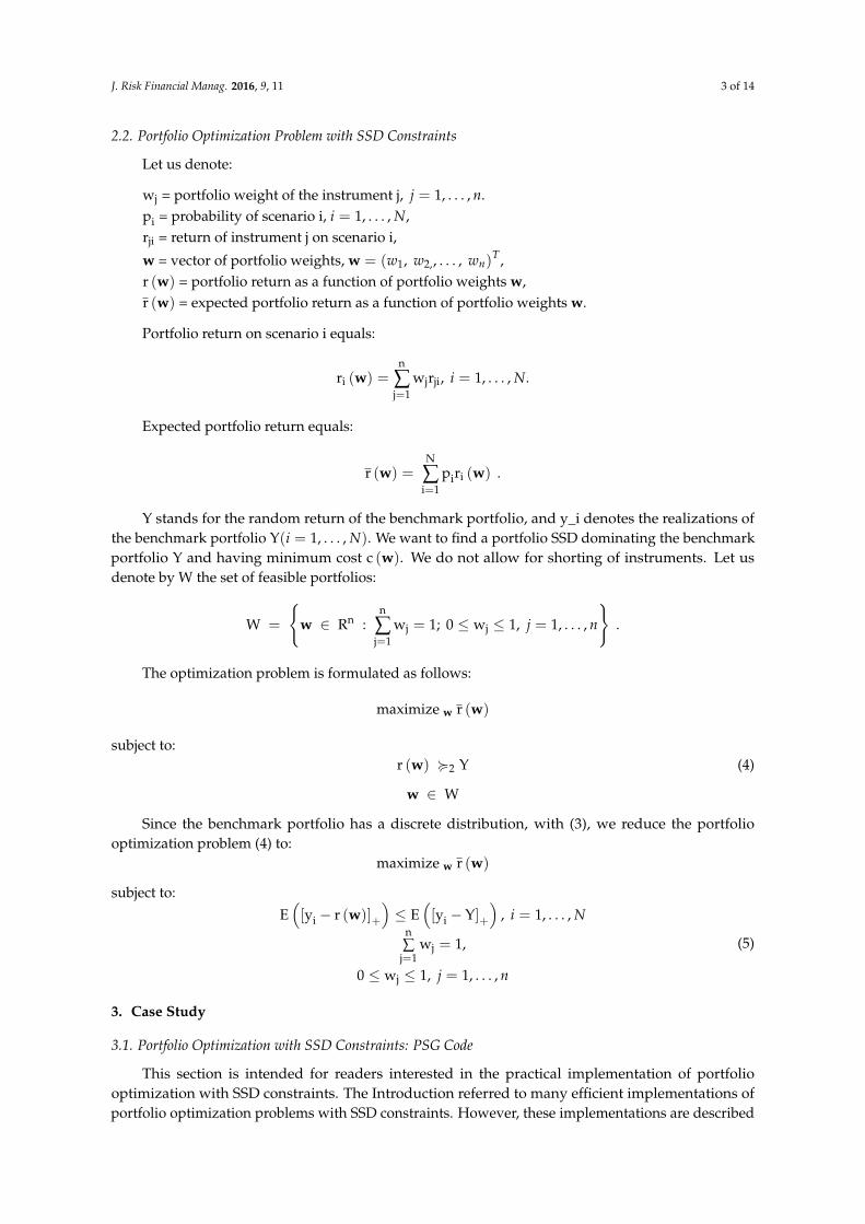
2.2. Portfolio Optimization Problem with SSD Constraints

Let us denote:

wj = portfolio weight of the instrument j, j = 1, . . . , n.pi = probability of scenario i, i = 1, . . . , N,rji = return of instrument j on scenario i,

w = vector of portfolio weights, w = (w1, w2,, . . . , wn)T ,

r (w) = portfolio return as a function of portfolio weights w,r (w) = expected portfolio return as a function of portfolio weights w.

Portfolio return on scenario i equals:

ri (w) =n

∑j=1

wjrji, i = 1, . . . , N.

Expected portfolio return equals:

r (w) =N

∑i=1

piri (w) .

Y stands for the random return of the benchmark portfolio, and y_i denotes the realizations ofthe benchmark portfolio Y(i = 1, . . . , N). We want to find a portfolio SSD dominating the benchmarkportfolio Y and having minimum cost c (w). We do not allow for shorting of instruments. Let usdenote by W the set of feasible portfolios:

W =

{w ∈ Rn :

n

∑j=1

wj = 1; 0 ≤ wj ≤ 1, j = 1, . . . , n

}.

The optimization problem is formulated as follows:

maximize w r (w)

subject to:r (w) <2 Y (4)

w ∈ W

Since the benchmark portfolio has a discrete distribution, with (3), we reduce the portfoliooptimization problem (4) to:

maximize w r (w)

subject to:E([yi − r (w)]+

)≤ E

([yi − Y]+

), i = 1, . . . , N

n∑

j=1wj = 1,

0 ≤ wj ≤ 1, j = 1, . . . , n

(5)

3. Case Study

3.1. Portfolio Optimization with SSD Constraints: PSG Code

This section is intended for readers interested in the practical implementation of portfoliooptimization with SSD constraints. The Introduction referred to many efficient implementations ofportfolio optimization problems with SSD constraints. However, these implementations are described


in research papers, and they are not readily available for portfolio optimization practitioners. Theoptimization problem (5) can be directly solved with PSG software without additional coding. PSG isfree for academic purposes. We posted at this link [22] several instances of solved problems (codes,data and solutions) in PSG Run-File (text) format and in PSG MATLAB (MathWorks, Natick, MA,USA) format. Below is the code for Problem (5) in PSG Run-File (text) format:Maximize

avg_g(matrix_sde)

Constraint: =1

Linear(matrix_budget)

MultiConstraint: ≤vector_ubound_sdpm_pen(vector_benchmark_sd, matrix_sde)

Box: ≥0, ≤1

Matrix “matrix_sde” contains a set of scenarios for instruments of the portfolio. The function“avg_g (matrix_sde)” calculates the average return of the portfolio defined by the matrix of scenarios.Linear function “linear (matrix_budget)” is used in the budget constraint; it is defined by the coefficientsin the matrix “matrix_budget”. SSD constraints are defined by the partial moment function “pm_pen(vector_benchmark_sd, matrix_sde)”, which depends on the “vector_benchmark_sd” containing thecomponents of the vector, yi, i = 1, . . . , N and the matrix of scenarios “matrix_sde” for instruments.

The vector “vector_ubound_sd” contains values E([yi − Y]+

), i = 1, . . . , N. The PSG code does not

have cycles; basically, it is presenting the problem (5) in analytic format with precoded functions.The website link [22] also contains data for the PSG MATLAB Toolbox for solving Problem (5) withdata imported from PSG text format. Furthermore, the MATLAB subroutine for Problem (5) wasautomatically generated from the PSG MATLAB Toolbox. A reader can solve Problem (5) by using thePSG MATLAB subroutine without learning the PSG capabilities. This MATLAB subroutine was usedin cycles in the out-of-sample simulations described in the following section.

Further, we discuss several numerical runs posted at the link [22]. The problems were solvedwith a PC with 3.14 GHz.

PROBLEM_1 describes three instances of portfolio optimization problems considered in thefollowing section. We found portfolios of stocks, which SSD dominate, the DAX, Dow Jones andS&P 100 indices. The instances have 3046, 3020 and 3020 scenarios (daily returns) and 26, 29 and90 variables (stocks from the indices included in the optimization), accordingly. The solution times are0.27, 0.05 and 0.21 s, accordingly. The PSG automatic procedure for removing redundant constraintsremoved 8, 0 and 2 constraints in the three instances, accordingly.

PROBLEM_2 describes a dataset with 30,000 scenarios considered in Fabian et al. [18]. Thisdataset contains many repeated (coinciding) nonlinear constraints. The PSG MultiConstraint setting inthe problem statement does automatic preprocessing and removes redundant and repeated constraints.The initial number of constraints (corresponding to the number of scenarios) is 30,000; the automaticPSG preprocessing of constraints reduces this number to 972. The solution time is 1.41 s.

PROBLEM_3 describes the same dataset as PROBLEM_2 with 30,000 scenarios, but all SSDconstraints are manually specified in the list. The list includes only 972 constraints, because wemanually removed repeated constraints. The solution time is 1.40 s.

PSG is free for academic purposes. The PSG solution times for similar dimensions are comparablewith the solution times of specialized algorithms described in Dentcheva and Ruszczynski [12,14],Dentcheva and Ruszczynski [16], Rudolf and Ruszczynski [13], Roman et al. [17] and Fabian et al. [18,19].The advantage of the described problems and PSG codes is that the numerical runs can be easilyverified with the data posted at the link [22]. Similar problems can be solved by replacing data in thematrices included in the PSG code. Since PSG codes are specified in analytic format, it is possible tomodify the codes without significant effort. For instance, additional constraints, such as “cardinality”,can be included in the problem statement to limit the number of securities in an optimal portfolio.


3.2. Mean-Variance Portfolios versus Portfolios with SSD Constraints

This section calculates mean-variance optimal portfolios and optimal portfolio with SSDconstraints specified by (5) for datasets of stocks from the Dow Jones, S&P 100 and DAX indices.

The first dataset includes stocks from the Dow Jones Index (DJI), and the DJ Index is consideredas a benchmark. Similar, the second and third datasets include stocks from the S&P 100 and DAXindices, and the S&P 100 and DAX indices were used as a benchmark, respectively. The data weredownloaded from Yahoo! Finance [23] and include 3020, 3020 and 3046 historical daily returns ofstocks from 1 January 2004 to 31 December 2015 for the DJ, S&P 100 and DAX indices respectively. Thelists of stocks in the indices are taken on 31 December 2015. Therefore, we considered only 29 stocksfrom the DJ Index, 90 stocks from the S&P 100 Index and 26 stocks from the DAX Index (Appendix Bcontains the list of the stocks selected for this paper). The stock returns on a daily basis, rji, werecalculated using the logarithm of the ratio of the stock adjusted closing prices, fi ,

rji = ln (fi/fi−1) .

We adjusted for splits the stocks prices of four companies from the DAX Index2. We considereddaily returns as equally probable scenarios. We calculated SSD-based portfolios described in (5),equally weighted, minimum variance and mean-variance portfolios with the constant and time-varyingcovariance matrices. Shorting is not allowed, and the sum of portfolio weights is equal to one,

n

∑j=1

wj = 1, wj ≥ 0, j = 1, . . . , n.

Here is a brief description of the portfolios:

i. Equally Weighted (EW)All stocks in the portfolio are equally weighted. Every stock has the same weight 1/n, where n isthe number of stocks in the portfolio.

ii. Minimum Variance (MinVar)The minimum variance portfolio has minimum variance without any constraint on portfolioreturn. Shorting is not allowed, and the sum of the portfolio weights is equal to one.

iii. Mean-Variance (Mean-Var)The mean-variance portfolio [1] uses the mean return and the variance of the stock returns.We considered Mean-Var problems having variance in the objective function and the expectedportfolio return of 8% per year in the constraint. Shorting is not allowed, and the sum of theportfolio weights is equal to one. We imposed a 0.2 upper bound constraint on the positions.

The numerical code was implemented with MATLAB R2012b [24]. We have used the PSGriskprog subroutine for MATLAB environment to solve MinVar and mean-variance portfolio problems.The calculations were performed on a notebook having a 2.5-GHz CPU and 8 GByte of RAM.

Table 1 shows the expected yearly returns of the portfolios for the considered approaches.

2 Deutsche Boerse AG (DB1.DE), Fresenius SE & Co. KGaA (FRE.DE), Infineon Technologies AG (IFX.DE) and Merck & Co.(MRK.DE) stock prices are adjusted for splits.


Table 1. Expected yearly returns of portfolios. EW, Equally Weighted; MinVar, Minimum Variance;Mean-Var, Mean-Variance; SSD, Second-Order Stochastic Dominance.

Portfolios DJI S&P 100 DAX

EW 0.04014 0.08509 0.09139MinVar 0.03419 0.08795 0.13362

Mean-Var 0.08327 0.08327 0.08327SSD 0.08762 0.24250 0.17922

Benchmark 0.04374 0.04287 0.08439

The SSD dominating portfolios can be used for actual investments. At least in the past, theseportfolios SSD dominated the corresponding indices. Moreover, the expected yearly return of theportfolio SSD dominating the DJ index equals 0.08762 and significantly exceeds the DJ index return inthis period. Similar observations are valid for the portfolio of S&P 100 and DAX indices; the expectedyearly returns of portfolio SSD dominating the benchmarks equal 0.24250 and 0.17922, respectively.

We compared solving times of SSD constrained optimization (using the PSG subroutine) withthe MinVar and Mean-Var approaches (using the PSG riskprog subroutine). Data loading and solvingtimes are given in Table 2; all problems are solved almost instantaneously.

Table 2. Loading and solving times (in seconds) with PSG in the MATLAB environment.

DJI S&P 100 DAX

Problem Loading Solving Loading Solving Loading Solving

SSD constrained (PSG code) 2.11 0.12 1.39 0.19 1.80 0.11MinVar (PSG riskprog) 0.27 0.01 0.33 0.01 0.26 0.01

Mean-Var (PSG riskprog) 0.38 0.01 0.44 0.02 0.38 0.01

3.3. Out-Of-Sample Simulations

We have evaluated the out-of-sample performance of several variants of mean-variance portfoliosand SSD constrained portfolios. We considered a time series framework where the estimation period(750 and 1000 days) is rolled over time. Portfolios are re-optimized on every first business day of themonth using the recent historical daily returns (750 or 1000). We kept constant positions during themonth. We set a 9% per year return constraint in Mean-Var problem. If the expected return 9% peryear is not feasible (in the beginning of the month), then we set a 6% expected return constraint, and ifwe still do not have feasibility, we reduce the expected return to 3% and then to 0%.

The classical mean-variance model considers the constant covariance matrix. For theout-of-sample simulations, we also considered the time-dependent covariance matrix using theConstant and Dynamic Conditional Correlation GARCH (CCC and DCC) models in the MinVar andMean-Var approaches. Further, we briefly describe the estimation procedure for the time-dependentcovariance matrices.

We considered constant and dynamic conditional correlation GARCH models for estimationof large time-dependent covariance matrices [25–28]. We estimated the time-dependent covariancematrix using Ht with a simple GARCH(1,1) model. The CCC-GARCH model assumes that correlationsare constant, R = ρij, and that covariances may change over time, and the time-dependent covariancematrix Ht is extracted from this model, where Ht = DtRDt. The DCC-GARCH model assumes thatcorrelations may change over time, and time-dependent covariance matrix Ht is extracted from themodel, where Ht = DtRtDt. Here, Dt is the diagonal matrix from a univariate GARCH model, andRt is the time-dependent correlation matrix [29]. This paper assumes the simplest conditional meanreturn equation where rj = N−1 ∑N

i=1 rji is the sample mean, and the deviation of returns (rt − r) isconditionally normal with zero mean and time-dependent covariance matrix Ht [30]. We used Ht

in MinVar and Mean-Var problems. For the estimation of the time-dependent covariance matrix,


we used the MFE Toolbox3 [31]. The difficulty in the estimation of the covariance matrices withthe DCC model is that the time-dependent conditional correlation matrix has to be positive definitefor all time moments. We observe that with small in-sample time intervals (such as 250 days), thevariance-covariance matrix may not be positive definite. Therefore, we have used 750 and 1000 daysas the in-sample periods.

Figures 1–6 show the out-of-sample compounded daily returns of the portfolios.



Figure 1. Compounded (on daily basis) returns of portfolios consisting of DJ stocks, t = 750. CCC,

Constant Conditional Correlation; DCC, Dynamic Conditional Correlation.

Figure 2. Compounded (on daily basis) returns of portfolios consisting of DJ stocks, t = 1000.

Figure 3. Compounded (on daily basis) returns of portfolios consisting of S&P 100 stocks, t = 750.

Figure 1. Compounded (on daily basis) returns of portfolios consisting of DJ stocks, t = 750. CCC,Constant Conditional Correlation; DCC, Dynamic Conditional Correlation.






Figure 3. Compounded (on daily basis) returns of portfolios consisting of S&P 100 stocks, t = 750.







Figure 3. Compounded (on daily basis) returns of portfolios consisting of S&P 100 stocks, t = 750. Figure 3. Compounded (on daily basis) returns of portfolios consisting of S&P 100 stocks, t = 750.

3 The CCC-GARCH and DCC-GARCH models are estimated by using MFE Toolbox for MATLAB software produced byKevin Sheppard.

J. Risk Financial Manag. 2016, 9, 11 8 of 14J. Risk Financial Manag. 2016, 9, 11 8 of 14

Figure 4. Compounded (on daily basis) returns of portfolios consisting of SP100 stocks, t = 1000.

Figure 5. Compounded (on daily basis) returns of portfolios consisting of DAX stocks, t = 750.


The out-of-sample performances of portfolios are represented in Tables 3–8. The tables include

yearly compounded portfolio returns for the years 2007–2015, the Total compounded Return (T_R)

and the Sharpe Ratio (Sh_R).

In Table 3 (DJ stocks, t = 750), the SSD constrained portfolio has the highest T_R (1.3961) and

Sh_R (0.5761) higher than all considered portfolios, except DCC Mean-Var and CCC Mean-Var.






















The out-of-sample performances of portfolios are represented in Tables 3–8. The tables includeyearly compounded portfolio returns for the years 2007–2015, the Total compounded Return (T_R)and the Sharpe Ratio (Sh_R).

In Table 3 (DJ stocks, t = 750), the SSD constrained portfolio has the highest T_R (1.3961) andSh_R (0.5761) higher than all considered portfolios, except DCC Mean-Var and CCC Mean-Var.


Table 3. Yearly compounded returns, Total compounded Return (T_R) and Sharpe Ratio (Sh_R) forDJ stocks (t = 750).

Portfolios 2007 2008 2009 2010 2011 2012 2013 2014 2015 TR Sh_R

EW 1.0514 0.8322 1.1166 1.0611 1.0280 1.0561 1.1243 1.0501 1.0010 1.3300 0.5398MinVar 1.0712 0.9169 1.0445 1.0147 1.0549 1.0433 1.0764 1.0253 0.9932 1.2557 0.4736

Mean-Var 1.0666 0.8344 1.0600 1.0565 1.0776 1.0393 1.0498 1.0728 1.016 1.2771 0.5303CCC MinVar 1.074 0.9285 0.9971 1.0085 1.0585 1.0295 1.0725 1.0429 1.0116 1.2363 0.4230

CCC Mean-Var 1.0805 0.8312 1.0499 1.0557 1.0742 1.0361 1.058 1.0722 1.0545 1.3252 0.5801DCC MinVar 1.0755 0.9209 1.0174 1.0076 1.0680 1.0310 1.0710 1.0475 1.0145 1.2725 0.4977

DCC Mean-Var 1.0814 0.8394 1.0623 1.0558 1.0785 1.0373 1.0636 1.0690 1.0538 1.3649 0.6422SSD 1.1202 0.8023 1.0873 1.1037 1.0109 1.0640 1.0827 1.0666 1.0421 1.3961 0.5761

Benchmark 1.0531 0.6157 1.1540 1.0958 1.0321 1.0652 1.2584 1.0688 0.9661 1.1715 0.1660

In Table 4 (DJ stocks, t = 1000), the SSD constrained portfolio has the highest T_R (1.5317) andSh_R (0.9008).

Table 4. Yearly compounded returns, Total compounded Return (T_R) and Sharpe Ratio (Sh_R) forDJ stocks (t = 1000).

Portfolios 2008 2009 2010 2011 2012 2013 2014 2015 TR Sh_R

EW 0.8322 1.1166 1.0611 1.0280 1.0561 1.1243 1.0501 1.0010 1.2650 0.4948MinVar 0.9132 1.0424 1.0162 1.0495 1.0583 1.0773 1.0309 0.9821 1.1719 0.3458

Mean-Var 0.8614 1.0930 1.0724 1.0832 1.0278 1.0512 1.0564 1.0021 1.2509 0.5384CCC MinVar 0.9515 1.0168 1.0184 1.0444 1.0427 1.0700 1.0592 1.0006 1.2169 0.4356

CCC Mean-Var 0.8129 1.0824 1.0692 1.0808 1.0382 1.0874 1.0657 1.0375 1.2692 0.5521DCC MinVar 0.9403 1.0236 1.0198 1.0513 1.0272 1.0719 1.0568 1.0075 1.2097 0.4303

DCC Mean-Var 0.8134 1.0791 1.0695 1.0840 1.0409 1.0848 1.0671 1.0494 1.2866 0.5785SSD 0.8416 1.0914 1.1057 1.0848 1.0449 1.1149 1.1013 1.0836 1.5317 0.9008

Benchmark 0.6157 1.1540 1.0958 1.0321 1.0652 1.2584 1.0688 0.9661 1.1124 0.1325

In Table 5 (S&P 100 stocks, t = 750), the SSD constrained portfolio has the highest T_R (3.0027)and Sh_R (0.9157).

Table 5. Yearly compounded returns, Total compounded Return (T_R) and Sharpe Ratio (Sh_R) forS&P 100 stocks (t = 750).


EW 1.0974 0.5795 1.2285 1.1490 0.9799 1.1736 1.3212 1.1218 0.9566 1.4633 0.3491MinVar 1.1968 0.7712 1.0044 1.1932 1.2649 1.0415 1.0066 1.2232 0.9882 1.7728 0.5230



DCC Mean-Var 1.1289 0.7363 1.1177 1.0927 1.2164 1.0040 1.1480 1.2090 1.0062 1.7312 0.5401SSD 1.3903 0.6163 1.2721 1.2017 1.0769 1.1489 1.4382 1.2542 1.0270 3.0027 0.9157

Benchmark 1.0255 0.5803 1.1532 1.0846 0.9839 1.1240 1.2667 1.0958 0.9908 1.1319 0.1342

In Table 6 (S&P 100 stocks, t = 1000), the SSD constrained portfolio has the highest T_R (1.9756)and Sh_R (0.7110).


Table 6. Yearly compounded returns, Total compounded Return (T_R) and Sharpe Ratio (Sh_R) forS&P 100 stocks (t = 1000).


EW 0.5795 1.2285 1.149 0.9799 1.1736 1.3212 1.1218 0.9566 1.3335 0.3054MinVar 0.7704 1.0417 1.1724 1.2598 0.9527 1.0614 1.1961 0.9929 1.4233 0.3610



DCC Mean-Var 0.7067 1.0691 1.1331 1.2236 1.1016 1.1708 1.2256 0.9758 1.6157 0.5068SSD 0.6225 1.1775 1.2189 1.1021 1.2194 1.2811 1.1809 1.0876 1.9756 0.7110

Benchmark 0.5803 1.1532 1.0846 0.9839 1.124 1.2667 1.0958 0.9908 1.1038 0.1231

In Table 7 (DAX stocks, t = 750), the SSD constrained portfolio has T_R (1.9364) higher than allconsidered portfolios, except CCC MinVar, and Sh_R (0.5164) higher than all considered portfolios,except CCC MinVar and DCC MinVar.

Table 7. Yearly compounded returns, Total compounded Return (T_R) and Sharpe Ratio (Sh_R) forDAX stocks (t = 750).


EW 1.1476 0.5003 1.2887 1.1687 0.8119 1.2526 1.2034 1.0217 1.1013 1.2582 0.1883MinVar 1.1195 0.5865 1.1608 1.0742 1.1487 1.1591 1.1537 1.0698 1.2479 1.7328 0.5114



DCC Mean-Var 1.1334 0.5993 0.9764 1.1661 1.1019 1.1105 1.0407 1.1002 1.2220 1.3685 0.2998SSD 1.2125 0.6067 0.9658 1.2335 0.9980 1.2800 1.3673 1.0785 1.1449 1.9364 0.5164

Benchmark 1.2082 0.5555 1.1891 1.1411 0.8181 1.2671 1.2414 1.0123 1.0656 1.3213 0.2248

In Table 8 (DAX stocks, t = 1000), the SSD constrained portfolio has T_R (1.4897) and Sh_R(0.39520) higher than all considered portfolios, except MinVar, CCC MinVar and DCC MinVar.

Table 8. Yearly compounded returns, Total compounded Return (T_R) and Sharpe Ratio (Sh_R) forDAX stocks (t = 1000).


EW 0.5003 1.2887 1.1687 0.8119 1.2526 1.2034 1.0217 1.1013 1.0561 0.0864MinVar 0.5959 1.147 1.0714 1.148 1.1541 1.1371 1.0747 1.2772 1.5177 0.4489



DCC Mean-Var 0.5688 1.1566 1.1647 1.0249 1.1996 1.0188 1.0792 1.1939 1.2427 0.2429SSD 0.6165 1.0476 1.2101 0.9354 1.2022 1.302 1.1201 1.1483 1.4897 0.3952

Benchmark 0.5555 1.1891 1.1411 0.8181 1.2671 1.2414 1.0123 1.0656 1.0718 0.1042

Appendix A shows the weights of SSD constrained portfolios at the last month of theout-of-sample period and portfolio weights with all in-sample data. Appendix B shows companycodes and names for the Dow Jones, SP500 and DAX indices.

4. Conclusions

This paper used Portfolio Safeguard (PSG) for portfolio optimization with SSD constraints.The algorithms are very efficient and can be run on a regular PC. The index portfolio optimization


instances have 3046, 3020 and 3020 scenarios (daily returns) and 26, 29 and 90 variables, accordingly.The solution times are 0.27, 0.05 and 0.21 s for these instances. Another instance with 76 variablesand 972 scenarios was optimized during 1.4 s. We have done out-of-sample simulations andcompared SSD constrained portfolios with the minimum variance and mean-variance portfolios.The portfolios were constructed from the stocks of the DJ, S&P 100 and DAX indices. The SSDconstrained portfolio demonstrated quite good out-of-sample performance and in the majority of caseshad the highest compounded return and Sharpe ratio (among the considered portfolios). We thinkthat SSD constrained optimization can be widely used in actual portfolio management, similar tomean-variance optimization.

Author Contributions: N. Fidan Keçeci wrote the paper and conducted the case study. V. Kuzmenko wasinvolved in proving mathematical statements and in software development for the case study. S. Uryasevprovided an overall guidance of the project.

Conflicts of Interest: The authors declare no conflict of interest.

Appendix A

Table A1. Weights of SSD constrained portfolios at the last month of the out-of-sample period andweights with all in-sample data. Stocks with zero positions for all periods (750, 1000 and 3020 days forDJ and S&P 100 and 750, 1000 and 3046 days for DAX) are skipped.

DJ Weights S&P100 Weights DAX Weights

Code 750Days

1000days

3020Days CODE 750

Days1000Days

3020Days Code 750

Days1000Days

3046Days

AAPL 0 0 0.2 AAPL 0 0 0.2 ADS.DE 0 0 0.075DIS 0.2 0.2 0.2 ALL 0 0.028 0 ALV.DE 0 0.0555 0HD 0.2 0.2 0.2 AMZN 0.021 0.016 0.031 BAYN.DE 0 0.066 0.2

MCD 0 0 0.2 BIIB 0 0 0.086 CON.DE 0.2 0.2 0.2MSFT 0.2 0.2 0 BMY 0.016 0 0 DAI.DE 0.063 0.132 0NKE 0.2 0.2 0.2 CVS 0 0.004 0 DB1.DE 0.137 0 0UNH 0.2 0.2 0 DIS 0.086 0.101 0 DPW.DE 0 0.2 0

GD 0.046 0 0 DTE.DE 0.2 0 0GILD 0.063 0.155 0.127 FRE.DE 0.2 0.2 0.2HD 0.021 0.2 0 SDF.DE 0 0 0.125

LMT 0.2 0.2 0.043 IFX.DE 0.2 0 0LOW 0.001 0.023 0 MRK.DE 0 0.1466 0.2MCD 0 0 0.113MO 0.186 0.172 0.2

MSFT 0.058 0 0NKE 0.2 0.005 0.2RTN 0.016 0.096 0

SBUX 0.045 0 0WBA 0.041 0 0

Appendix B

Table B1. DJ and DAX company codes and names.

DAX DJ

Code Name Code Name

1 EOAN.DE E.ON SE AAPL Apple Inc.2 ADS.DE Adidas AG AXP American Express Company3 ALV.DE Allianz SE BA The Boeing Company4 BAS.DE BASF SE CAT Caterpillar Inc.5 BAYN.DE Bayer AG CSCO Cisco Systems, Inc.6 BEI.DE Beiersdorf AG CVX Chevron Corporation7 BMW.DE Bayerische Mot. Werke Aktienges. DD E. I. du Pont de Nemours and Company


Table B1. Cont.

DAX DJ

Code Name Code Name

8 CBK.DE Commerzbank AG DIS The Walt Disney Company9 CON.DE Continental Aktiengesellschaft GE General Electric Company10 DAI.DE Daimler AG GS The Goldman Sachs Group, Inc.11 DB1.DE Deutsche Boerse AG HD The Home Depot, Inc.12 DBK.DE Deutsche Bank AG IBM Int. Business Machines Corporation13 DPW.DE Deutsche Post AG INTC Intel Corporation14 DTE.DE Deutsche Telekom AG JNJ Johnson & Johnson15 FME.DE Fres. Med. Care AG & Co. KGAA JPM JPMorgan Chase & Co.16 FRE.DE Fresenius SE & Co. KGaA KO The Coca-Cola Company17 HEI.DE Heidelberg Cement AG MCD McDonald’s Corp.18 SDF.DE K + S Aktiengesellschaft MMM 3M Company19 IFX.DE Infineon Technologies AG MRK Merck & Co. Inc.20 LHA.DE Deutsche Luft. Aktiengesellschaft MSFT Microsoft Corporation21 LIN.DE Linde Aktiengesellschaft NKE Nike, Inc.22 MRK.DE Merck KGaA PFE Pfizer Inc.23 MUV2.DE Münchener R.G.A. PG The Procter & Gamble Company24 SAP.DE SAP SE TRV The Travelers Companies, Inc.25 SIE.DE Siemens Aktiengesellschaft UNH UnitedHealth Group Incorporated26 TKA.DE ThyssenKrupp AG UTX United Technologies Corporation27 VZ Verizon Communications Inc.28 WMT Wal-Mart Stores Inc.29 XOM Exxon Mobil Corporation

Table B2. S&P 100 company codes and names.

Code Name Code Name

1 AAPL Apple Inc. IBM International Business Machines2 ABT Abbott Laboratories INTC Intel Corporation3 ACN Accenture plc JNJ Johnson & Johnson Inc.4 AIG American International Group Inc. JPM JP Morgan Chase & Co5 ALL Allstate Corp. KO The Coca-Cola Company6 AMGN Amgen Inc. LLY Eli Lilly and Company7 AMZN Amazon.com LMT Lockheed-Martin8 APA Apache Corp. LOW Lowe’s9 APC Anadarko Petroleum Corp. MCD McDonald’s Corp.10 AXP American Express Inc. MDLZ Mondelez International11 BA Boeing Co. MDT Medtronic Inc.12 BAC Bank of America Corp MET MetLife Inc.13 BAX Baxter International Inc. MMM 3M Company14 BIIB Biogen Idec MO Altria Group15 BK Bank of New York MON Monsanto16 BMY Bristol-Myers Squibb MRK Merck & Co.17 BRK.B Berkshire Hathaway MS Morgan Stanley18 C Citigroup Inc. MSFT Microsoft19 CAT Caterpillar Inc. NKE Nike20 CL Colgate-Palmolive Co. NOV National Oilwell Varco21 CMCSA Comcast Corporation ORCL Oracle Corporation22 COF Capital One Financial Corp. OXY Occidental Petroleum Corp.23 COP ConocoPhillips PEP PepsiCo Inc.24 COST Costco PFE Pfizer Inc.25 CSCO Cisco Systems PG Procter & Gamble Co26 CVS CVS Caremark QCOM Qualcomm Inc.27 CVX Chevron RTN Raytheon Company28 DD DuPont SBUX Starbucks Corporation29 DIS The Walt Disney Company SLB Schlumberger30 DOW Dow Chemical SO Southern Company21 EBAY eBay Inc. SPG Simon Property Group, Inc.32 EMC EMC Corporation T AT&T Inc.33 EMR Emerson Electric Co. TGT Target Corp.34 EXC Exelon TWX Time Warner Inc.35 F Ford Motor TXN Texas Instruments36 FCX Freeport-McMoran UNH UnitedHealth Group Inc.


Table B2. Cont.

Code Name Code Name

37 FDX FedEx UNP Union Pacific Corp.38 FOXA Twenty-First Century Fox, Inc. UPS United Parcel Service Inc.39 GD General Dynamics USB US Bancorp40 GE General Electric Co. UTX United Technologies Corp41 GILD Gilead Sciences VZ Verizon Communications Inc.42 GS Goldman Sachs WBA Walgreens Boots Alliance43 HAL Halliburton WFC Wells Fargo44 HD Home Depot WMT Wal-Mart45 HON Honeywell XOM Exxon Mobil Corp

References

1. Markowitz, H. Portfolio Selection. J. Financ. 1952, 7, 77–91. [CrossRef]2. Mann, H.B.; Whitney, D.R. On a Test of Whether one of Two Random Variables is Stochastically Larger than

the Other. Ann. Math. Stat. 1947, 18, 50–60. [CrossRef]3. Lehmann, E.L. Ordered Families of Distributions. Ann. Math. Stat. 1955, 26, 399–419. [CrossRef]4. Levy, H. Stochastic Dominance: Investment Decision Making under Uncertainty; Springer: Berlin, Germany, 2015.5. Muller, A.; Stoyan, D. Comparison Methods for Stochastic Models and Risks; John Wiley & Sons: Chichester,

UK, 2002.6. Shaked, M.; Shanthikumar, J.G. Stochastic Orders and Their Applications; Academic Press: Boston, MA,

USA, 1994.7. Whitmore, G.A.; Findlay, M.C. (Eds.) Stochastic Dominance: An Approach to Decision-Making Under Risk;

Lexington Books: Lanham, MD, USA, 1978.8. Lizyayev, A. Stochastic dominance efficiency analysis of diversified portfolios: Classification, comparison

and refinements. Ann. Oper. Res. 2012, 196, 391–410. [CrossRef]9. Ogryczak, W.; Ruszczynski, A. Dual Stochastic Dominance and Related Mean-Risk Models. SIAM J. Optim.

2002, 13, 60–78. [CrossRef]10. Dentcheva, D.; Ruszczynski, A. Optimization with Stochastic Dominance Constraints. SIAM J. Optim. 2003,

14, 548–566. [CrossRef]11. Kuosmanen, T. Efficient Diversification According to Stochastic Dominance Criteria. Manag. Sci. 2004, 50,

1390–1406. [CrossRef]12. Dentcheva, D.; Ruszczynski, A. Portfolio optimization with stochastic dominance constraints. J. Bank. Financ.

2006, 30, 433–451. [CrossRef]13. Rudolf, G.; Ruszczynski, A. Optimization Problems with Second Order Stochastic Dominance Constraints:

Duality, Compact Formulations, and Cut Generation Methods. SIAM J. Optim. 2008, 19, 1326–1343.[CrossRef]

14. Dentcheva, D.; Ruszczynski, A. Inverse stochastic dominance constraints and rank dependent expectedutility theory. Math. Program. 2006, 108, 297–311. [CrossRef]

15. Kopa, M.; Chovanec, P. A second-order stochastic dominance portfolio efficiency measure. Kybernetika 2008,44, 243–258.

16. Dentcheva, D.; Ruszczynski, A. Inverse cutting plane methods for optimization problems with second-orderstochastic dominance constraints. Optimization 2010, 59, 323–338. [CrossRef]

17. Roman, D.; Darby-Dowman, K.; Mitra, G. Portfolio construction based on stochastic dominance and targetreturn distributions. Math. Program. Ser. B 2006, 108, 541–569. [CrossRef]

18. Fabian, C.I.; Mitra, G.; Roman, D.; Zverovich, V. An enhanced model for portfolio choice with SSD criteria:A constructive approach. Quant. Financ. 2011, 11, 1525–1534. [CrossRef]

19. Fabian, C.I.; Mitra, G.; Roman, D. Processing second-order stochastic dominance models using cutting-planerepresentations. Math. Program. 2011, 130, 33–57. [CrossRef]

20. American Optimal Decisions, Inc. Portfolio Safeguard (PSG). Available online: http://aorda.com/index.php/portfolio-safeguard/ (accessed on 31 December 2015).

http://dx.doi.org/10.1111/j.1540-6261.1952.tb01525.x

http://dx.doi.org/10.1214/aoms/1177730491

http://dx.doi.org/10.1214/aoms/1177728487

http://dx.doi.org/10.1007/s10479-012-1123-4

http://dx.doi.org/10.1137/S1052623400375075

http://dx.doi.org/10.1137/S1052623402420528

http://dx.doi.org/10.1287/mnsc.1040.0284

http://dx.doi.org/10.1016/j.jbankfin.2005.04.024

http://dx.doi.org/10.1137/070702473

http://dx.doi.org/10.1007/s10107-006-0712-x

http://dx.doi.org/10.1080/02331931003696350

http://dx.doi.org/10.1007/s10107-006-0722-8

http://dx.doi.org/10.1080/14697680903493607

http://dx.doi.org/10.1007/s10107-009-0326-1

http://aorda.com/index.php/portfolio-safeguard/

http://aorda.com/index.php/portfolio-safeguard/


21. Ogryczak, W.; Ruszczynski, A. From stochastic dominance to mean-risk models: Semideviations as riskmeasures. Eur. J. Oper. Res. 1999, 116, 33–50. [CrossRef]

22. Case Study: Portfolio Optimization with Second-Order Stochastic Dominance Constraints. Available online:http://www.ise.ufl.edu/uryasev/research/testproblems/financial_engineering/portfolio-optimization-with-second-orders-stochastic-dominance-constraints/ (17 August 2016).

23. Yahoo! Finance. Available online: https://www.finance.yahoo.com (accessed on 31 December 2015).24. MATLAB R2012b, The MathWorks, Inc.: Natick, Massachusetts, United States, 2012.25. Engle, R.F.; Sheppard, K. Theoretical and Empirical Properties of Dynamic Conditional Correlation Multivariate

GARCH; NBER Working Paper No. w8554; National Bureau of Economic Research: Cambridge, MA,USA, 2001.

26. He, C.; Terasvirta, T. An Extended Constant Conditional Correlation GARCH Model and Its Fourth-MomentStructure. Econom. Theory 2004, 20, 904–926. [CrossRef]

27. Tse, Y.K.; Tsui, A.K.C. A Multivariate Generalized Autoregressive Conditional Heteroscedasticity Modelwith TimeVarying Correlations. J. Bus. Econ. Stat. 2002, 20, 351–362. [CrossRef]

28. Engle, R. Dynamic Conditional Correlation: A Simple Class of Multivariate Generalized AutoregressiveConditional Heteroskedasticity Models. J. Bus. Econ. Stat. 2002, 20, 339–350. [CrossRef]

29. Bauwens, L.; Laurent, S.; Rombouts, J.V. Multivariate GARCH models: A survey. J. Appl. Economy. 2006, 21,79–109. [CrossRef]

30. Alexander, C. Market Risk Analysis: Practical Financial Econometrics; John Willey & Sons: Hoboken, NJ,USA, 2008.

31. Kevin Sheppard Oxford-Man Institute of Quantitative Finance, Oxford, U.K. MFE Toolbox. Available online:https://www.kevinsheppard.com/MFE_Toolbox (accessed on 12 October 2015).

© 2016 by the authors; licensee MDPI, Basel, Switzerland. This article is an open accessarticle distributed under the terms and conditions of the Creative Commons Attribution(CC-BY) license (http://creativecommons.org/licenses/by/4.0/).

http://dx.doi.org/10.1016/S0377-2217(98)00167-2

http://www.ise.ufl.edu/uryasev/research/testproblems/financial_engineering/portfolio-optimization-with-second-orders-stochastic-dominance-constraints/

http://www.ise.ufl.edu/uryasev/research/testproblems/financial_engineering/portfolio-optimization-with-second-orders-stochastic-dominance-constraints/

https://www.finance.yahoo.com

http://dx.doi.org/10.1017/S0266466604205059

http://dx.doi.org/10.1198/073500102288618496

http://dx.doi.org/10.1198/073500102288618487

http://dx.doi.org/10.1002/jae.842

https://www.kevinsheppard.com/MFE_Toolbox

http://creativecommons.org/

http://creativecommons.org/licenses/by/4.0/.

portfolios dominating indices: optimization with second

Documents