portfolio turnpikes - washington university in st. louisthe portfolio turnpike models. portfolio...

Portfolio TurnpikesPhilip H. DybvigWashington University in Saint Louis

L. C. G. RogersUniversity of Bath

Kerry BackWashington University in Saint Louis

Portfolio turnpike theorems show that if preferences at large wealth levels aresimilar to power utility, then the investment strategy converges to the powerutility strategy as the horizon increases. We state and prove two simple andgeneral portfolio turnpike theorems. Unlike existing literature, our main resultdoes not assume independence of returns and depends only on discounting offuture cash flows. We also provide a critique of portfolio turnpike results, basedon the observations that (1) the time required for convergence is often too large tobe relevant, and (2) there is no convergence for consumption withdrawal problems.

Turnpike theorems in finance make a seductive promise: when the horizonis long, we can obtain essentially optimal portfolio weights by solving a rel-atively simple problem assuming power utility with a shape similar to thatof the correct utility function at large wealth levels. Although the literaturecontains a number of these results with different technical variations, themain assumptions that are common in the existing literature are (1) returnsare independent over time (and in most articles i.i.d.), and (2) investmentscan grow over time because the riskless rate is positive. It is the purpose ofthis article to provide a critical examination of this literature and provide anew perspective on these results. There are two main contributions in this ar-ticle. One is to provide a simple and general turnpike result that helps to putthe literature in perspective. The second is to provide numerical examplesthat indicate whether convergence is fast enough for practical use. Our mainfindings are (1) it is the growth of the economy as reflected in interest ratesor discount bond prices, not independence, that is critical for the results, and(2) convergence is too slow to be of practical interest, provided we assumereal rates of interest are small enough to be plausible. We conclude thatwhile portfolio turnpike theorems enhance our intuition and understandingof portfolio problems, they are not particularly useful in practice.

The authors are grateful for partial support by EPSRC grant GR/K00448. Address correspondence toPhilip H. Dybvig, Washington University Olin School, Campus Box 1133, 1 Brookings Dr., St. Louis,MO 63130-4899, or e-mail: [email protected].

The Review of Financial StudiesSpring 1999 Vol. 12, No. 1, pp. 165–195c© 1999 The Review of Financial Studies 0893-9454/99/$1.50

The Review of Financial Studies / v 12 n 1 1999

The term “turnpike theorem” has its origins in growth theory. Accordingto Dorfman, Samuelson, and Solow (1958),

It is, in a sense, the single most effective way for the system to grow, sothat if we are planning long-run growth, no matter where we start andwhere we desire to end up, it will pay in the intermediate stages to get intoa growth phase of this kind. It is exactly like a turnpike paralleled by a net-work of minor roads. There is a fastest route between any two points; andif origin and destination are close together and far from the turnpike, thebest route may not touch the turnpike. But if origin and destination are farenough apart, it will always pay to get on to the turnpike and cover distanceat the best rate of travel, even if this means adding a little mileage at eitherend. The best intermediate capital configuration is one which will growmost rapidly; even if it is not the desired one, it is temporarily optimal.

Based on this analogy, these results are called turnpike theorems, and asignificant literature has grown out of this idea. For an agent maximizingexpected utility of terminal wealth at a distant horizon, portfolio turnpiketheorems say that the agent’s optimal portfolio is insensitive to propertiesof the utility function at low wealth levels. Such results always assume amarket which is growing indefinitely (as they clearly must); it is then notsurprising that the values of the utility at low wealth levels are unimportant,as the agent can always get away from these low levels simply by followingthe growing market. In particular, portfolio turnpike theorems say that for allutility functions that are similar (in some suitably defined sense) to a powerutility function at large wealth levels, the optimal portfolio strategy spendsmost of its time over a large horizon following a portfolio strategy similarto the portfolio strategy of the power utility function, a neighborhood ofwhich is the turnpike.

To introduce turnpike theorems without the full weight of the formalmodel, we provide examples in Section 1. These examples form the basis ofour critique of turnpike results. Our critique looks at two separate problems.First, the optimal path may not lie near the turnpike unless one has anextremely long horizon. Examples with reasonable parameter values suggestthat it may take a horizon in excess of 50 or 100 years before the optimalportfolio choice is close to its asymptotic value, even if the utility functionis identical above the initial wealth level. The rate of interest, properlyinterpreted as a real rate of interest, seems to be a critical parameter indetermining the rate of convergence. Faster convergence would require usto assume an unreasonably large real rate of interest. The slow convergencesuggests that the portfolio turnpike results are of little practical import:using the asymptotically correct strategy may be far from optimal, even atthe largest horizons likely to be encountered in practice.

The second problem with the turnpike results is that they do not hold forconsumption-withdrawal problems. While many investment problems may

166

Portfolio Turnpikes

have overall horizons that are very large or even unbounded (such as themanagement of a university endowment), these problems involve ongoingwithdrawals for consumption, which are assumed away by the structure ofthe portfolio turnpike models. Portfolio turnpike theorems can be relied onas a useful approximation only when the time until the first consumptionwithdrawal is very large, and this is unlikely to be encountered in practice.

In Section 2 we describe the formal model and state our main result,Theorem 1; this is a comparison theorem that contains many existing resultsin the literature. We show that if two agents have similar marginal utilities atlarge consumption levels, they must have nearly the same wealth process andportfolio strategy at early times when the horizon is distant. The intuition forour main result is simple: assuming positive interest rates (or something likethat), our portfolio outgrows the low wealth levels for which the two utilityfunctions are significantly different. If all reinvestment were at the risklessrate, it would be obvious that it is the shape of the utility function at largewealth levels that governs the indirect utility function at short horizons.What is more subtle is to see that the states of nature with low optimalconsumption at the end, while occuring with positive probability given thepresence of risk taking, are not very significant economically, and have asmall influence on initial portfolio choice. From the previous literature itmight seem that this follows from independence of returns and some sort oflaw of large numbers; our results do not require independence and thereforewe conclude that it is discounting alone, not discounting combined withindependence, that drives turnpike results.

This main result assumes complete markets in a continuous-time model;the local means and variances of security returns can follow fairly generaladapted processes. We impose regularity through existence of moments ofthe state price density rather than through specific assumptions about thereturns themselves, such as assuming that returns are independent over timeor that stock prices are diffusions. We consider the portfolio strategies oftwo agents, and unlike the literature, we do not assume that either agentnecessarily has constant relative risk aversion. Utility functions satisfy auniform continuity property which certainly holds if the relative risk aver-sion is bounded above and below.

One result which is not covered by Theorem 1 is that of Hubermanand Ross (1983). Apart from the inessential difference of being stated indiscrete time, their result uses a weaker notion of equivalence of utilities(regular variation of marginal utilities, with the same exponent), but it makesa stronger assumption (independence over time) about returns. Under thecontinuous-time analogues of these assumptions, we prove (Theorem 2)the continuous-time analogue of the Huberman–Ross result. This is the firstcontinuous-time result of this sort, and it provides a bridge between thediscrete- and continuous-time literatures. One innovation in this result isthat we assume much less smoothness on preferences than do Huberman

167


and Ross or the rest of the literature. This is possible because of a result thatshows that there is a smooth utility function with a slightly different horizonthat has exactly the same portfolio choice and wealth process. This resultpermits us to apply the results assuming smooth preferences to preferenceswith kinks.

The literature on portfolio turnpike theorems includes discrete-time mod-els [Mossin (1968), Leland (1972), Hakansson (1974), Huberman and Ross(1983)] and continuous-time models [Cox and Huang (1992), Huang andZariphopoulou (forthcoming)]. All of these articles assume i.i.d. returns,with the exception of Huberman and Ross. Huberman and Ross assumereturns are independent across periods, with bounded support. We do notassume independence in our main result. In all of the previous literature,it was also assumed that the reference utility function has constant relativerisk aversion, which we have not assumed [instead, we assume the weakeruniform continuity condition of Equation (27)].

There are different assumptions in the literature regarding how the utilityfunction converges to the reference utility function at large wealth levels.In order to compare our Equation (26), made in Section 2, to the previousliterature, we need to specialize our model by assuming the reference utilityfunction has constant relative risk aversion. With this specialization, Equa-tion (26) is the same assumption made by Huang and Zariphopoulou and isstrictly more general than the assumptions of Mossin, Leland, and Cox andHuang. However, it is less general than that of Huberman and Ross, andapparently simply different from Hakansson’s.

The proofs of both Theorem 1 and Theorem 2 are relegated to an ap-pendix, although the text does outline the main ideas of the proofs. Con-vergence of relative risk aversion implies regular variation, which in turnimplies the regularity condition of Theorem 1, which shows that many re-sults in the literature can be read off from our main results. These resultsand related comparisons are shown in Lemma 1. Section 3 closes the article,and the Appendix contains the proofs.

1. Examples and Critique

The portfolio turnpike results tell us that, given utility functions that areasymptotically similar at large wealth, the portfolio strategies are asymp-totically similar at large horizons. This section uses examples to help thereader to develop an intuition for the turnpike results and their limitations.

The major limitations of the turnpike results may be summarized intwo critiques: first, examples show that, with reasonable parameter values(especially when the real riskless rate is reasonably small), the convergencemay be slow (even when the utility function differs from a power functiononly at levels below the initial wealth, we may not be near convergence evenwith a horizon as long as 100 years!); and, second, we should not expect any

168

Portfolio Turnpikes

turnpike results in consumption withdrawal problems. This second critiqueis implicit or explicit in many of the turnpike articles, but it is worthy ofattention, especially in combination with the other critique: no consumptionwithdrawal over 50 years seems unusual.

In later sections of the article, we will specify our formal model moreprecisely, but for now we will present just enough notation to be able topresent the examples without proof. Throughout the article, we will assumea continuous-time model in which the underlying uncertainty is generated bya standard Wiener process that may be multidimensional. For the exampleswe will specialize this to fixed coefficients in a world with a one-dimensionalWiener process and a single riskless asset. We will taker to be the fixedriskless rate,µ to be the fixed mean return on the risky asset, andσ tobe the fixed standard deviation of return on the risky asset. As is wellknown, the effective budget constraint in this problem can be written asW0 = E[CξT ], where W0 is initial wealth,C is consumption,T is thehorizon, andξt = exp(−(r − γ 2/2)t − γ Zt ) for γ ≡ (µ− r )/σ . Finally,we choose in this section to remain vague on the definition of when twoutility functions are “similar at large wealth levels.” Suffice it to say thatthere are a number of definitions in the literature and that our examples haveutility functions that are similar whatever definition we use (although as aninessential matter they may not satisfy regularity assumed by the literatureat low wealth levels). Formal definitions are given in Section 2.

Example 1Here we take utilities

u0(C) ≡{

C1−R

1−R for C > 0−∞ for C ≤ 0

(1)

and

u1(C) ≡{(C−K )1−R

1−R for C > K−∞ for C ≤ K

(2)

whereK is the translation andR> 0 is the shared risk-aversion parameter.1

It is easy to verify that these two utility functions are similar in the sense ofEquation (26) given that theR’s are the same.

With u0 and u1 defined in this way, the solutions for the two utilityfunctions are closely related for reasons given by Cass and Stiglitz (1970).By a simple change of variables that converts the problem for one utility

1 Formally, whenK is negative we want to relax the nonnegative wealth constraint in a way that does notcreate an arbitrage so negative consumption can be permitted, for example, by some sort ofL p integrabilitycondition or a looser lower bound on wealth. Addressing this purely technical issue in detail would takeus too far afield of our main purpose.

169


Table 1Distance from the turnpike: positively translated CRRA

Years to maturityr 1 2 5 10 25 50 100

2% 96.12 92.45 82.62 69.31 43.53 22.54 7.264% 92.45 85.72 69.31 50.41 22.54 7.26 0.926% 88.99 79.68 58.83 37.82 12.56 2.55 0.128% 85.72 74.24 50.41 28.98 7.26 0.92 0.02

10% 82.62 69.31 43.53 22.54 4.28 0.34 0.00

The table gives the percentage error from using the asymptotic valueinstead of the optimum. For example, if it is optimal to invest 50%of wealth in the risky asset, an entry of 10.00 in the table implies theasymptotic rule would give 55% instead. The utility function is constantrisk aversion translated by 50% of initial wealth, that is,K = W0/2.The entries in this table are not sensitive toµ (if not equal tor ), σ (if notzero), orR (if positive). The annual (real) riskless rater and the numberof years to maturityT are varied in the table.

function into the other we have that any solution has the property that

C1T = K + W0− K E[ξT ]

W0C0T (3)

relates the two consumptions. If we taker to be constant (as we will for thecalculations), the portfolio investment needed to achieveK uses only theriskless asset, and the portfolios are related by

θ1t;T = W0− Ke−rT

W0θ0t;T , (4)

since the discount factor isE[ξT ] = e−rT whenr is constant. By the turnpiketheorem (or by direct computation), the two portfolio strategies convergeasT increases. According to this result, the relative error for agent 1 fromusing the asymptotic risky asset portfolioθ0t;T instead of the correct one,defined to be

(θ0t;T − θ1t;T )/θ1t;T ,

is given byK/(W0erT − K ), independent ofR and the parameters of therisky asset return processes.

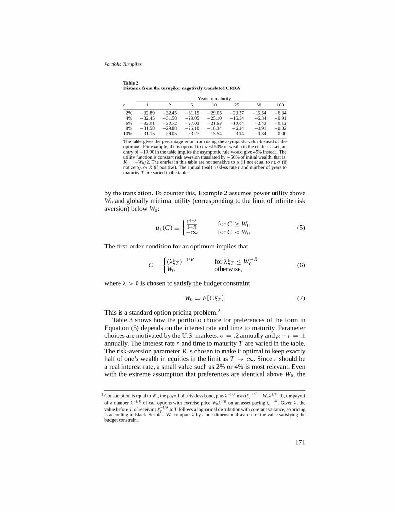
For power utility translated by 50% of initial wealth, Tables 1 and 2 showthe percentage error we would make in choosing what is optimal for thepower utility (as is asymptotically correct as the horizon increases) insteadof what is actually optimal. At reasonable real interest rates (2% or 4%),convergence is probably too slow to make this a useful approximation.

Example 2The class of examples based on translated power utility is very suggestivethat convergence tends to be slow. However, one weakness of this class ofexamples is that the entire utility function is changed (at least somewhat)

170

Portfolio Turnpikes

Table 2Distance from the turnpike: negatively translated CRRA


2% −32.89 −32.45 −31.15 −29.05 −23.27 −15.54 −6.344% −32.45 −31.58 −29.05 −25.10 −15.54 −6.34 −0.916% −32.01 −30.72 −27.03 −21.53 −10.04 −2.43 −0.128% −31.58 −29.88 −25.10 −18.34 −6.34 −0.91 −0.02

10% −31.15 −29.05 −23.27 −15.54 −3.94 −0.34 0.00

The table gives the percentage error from using the asymptotic value instead of theoptimum. For example, if it is optimal to invest 50% of wealth in the riskless asset, anentry of−10.00 in the table implies the asymptotic rule would give 45% instead. Theutility function is constant risk aversion translated by−50% of initial wealth, that is,K = −W0/2. The entries in this table are not sensitive toµ (if not equal tor ), σ (ifnot zero), orR (if positive). The annual (real) riskless rater and number of years tomaturityT are varied in the table.

by the translation. To counter this, Example 2 assumes power utility aboveW0 and globally minimal utility (corresponding to the limit of infinite riskaversion) belowW0:

u1(C) ≡{

C1−R

1−R for C ≥ W0

−∞ for C < W0(5)

The first-order condition for an optimum implies that

C ={(λξT )

−1/R for λξT ≤ W−R0

W0 otherwise,(6)

whereλ > 0 is chosen to satisfy the budget constraint

W0 = E[CξT ]. (7)

This is a standard option pricing problem.2

Table 3 shows how the portfolio choice for preferences of the form inEquation (5) depends on the interest rate and time to maturity. Parameterchoices are motivated by the U.S. markets:σ = .2 annually andµ− r = .1annually. The interest rater and time to maturityT are varied in the table.The risk-aversion parameterR is chosen to make it optimal to keep exactlyhalf of one’s wealth in equities in the limit asT → ∞. Sincer should bea real interest rate, a small value such as 2% or 4% is most relevant. Evenwith the extreme assumption that preferences are identical aboveW0, the

2 Consumption is equal toW0, the payoff of a riskless bond, plusλ−1/R max(ξ−1/RT −W0λ

1/R,0), the payoff

of a numberλ−1/R of call options with exercise priceW0λ1/R on an asset payingξ−1/R

T . Givenλ, the

value beforeT of receivingξ−1/RT atT follows a lognormal distribution with constant variance, so pricing

is according to Black–Scholes. We computeλ by a one-dimensional search for the value satisfying thebudget constraint.

171


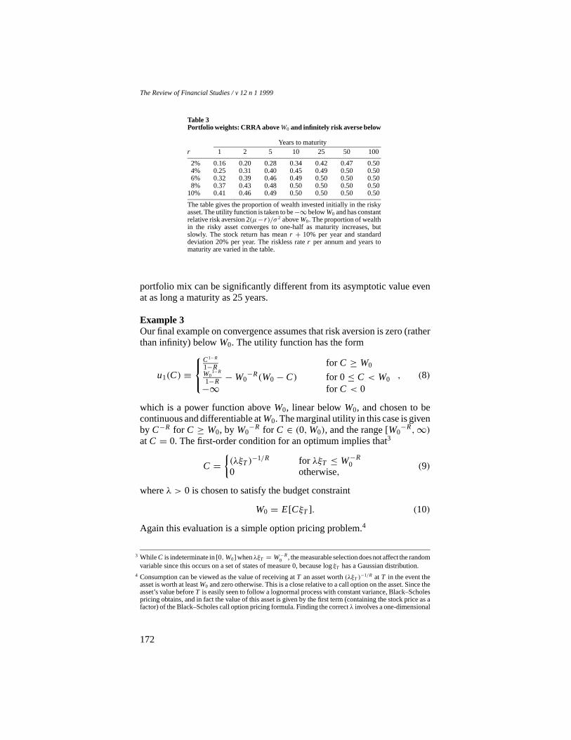
Table 3Portfolio weights: CRRA aboveW0 and infinitely risk averse below


2% 0.16 0.20 0.28 0.34 0.42 0.47 0.504% 0.25 0.31 0.40 0.45 0.49 0.50 0.506% 0.32 0.39 0.46 0.49 0.50 0.50 0.508% 0.37 0.43 0.48 0.50 0.50 0.50 0.50

10% 0.41 0.46 0.49 0.50 0.50 0.50 0.50

The table gives the proportion of wealth invested initially in the riskyasset. The utility function is taken to be−∞belowW0 and has constantrelative risk aversion 2(µ− r )/σ 2 aboveW0. The proportion of wealthin the risky asset converges to one-half as maturity increases, butslowly. The stock return has meanr + 10% per year and standarddeviation 20% per year. The riskless rater per annum and years tomaturity are varied in the table.

portfolio mix can be significantly different from its asymptotic value evenat as long a maturity as 25 years.

Example 3Our final example on convergence assumes that risk aversion is zero (ratherthan infinity) belowW0. The utility function has the form

u1(C) ≡

C1−R

1−R for C ≥ W0W0

1−R

1−R −W0−R(W0− C) for 0≤ C < W0

−∞ for C < 0

, (8)

which is a power function aboveW0, linear belowW0, and chosen to becontinuous and differentiable atW0. The marginal utility in this case is givenby C−R for C ≥ W0, by W0

−R for C ∈ (0,W0), and the range [W0−R,∞)

atC = 0. The first-order condition for an optimum implies that3

C ={(λξT )

−1/R for λξT ≤ W−R0

0 otherwise,(9)

whereλ > 0 is chosen to satisfy the budget constraint

W0 = E[CξT ]. (10)

Again this evaluation is a simple option pricing problem.4

3 WhileC is indeterminate in [0,W0] whenλξT = W−R0 , the measurable selection does not affect the random

variable since this occurs on a set of states of measure 0, because logξT has a Gaussian distribution.4 Consumption can be viewed as the value of receiving atT an asset worth(λξT )

−1/R at T in the event theasset is worth at leastW0 and zero otherwise. This is a close relative to a call option on the asset. Since theasset’s value beforeT is easily seen to follow a lognormal process with constant variance, Black–Scholespricing obtains, and in fact the value of this asset is given by the first term (containing the stock price as afactor) of the Black–Scholes call option pricing formula. Finding the correctλ involves a one-dimensional

172

Portfolio Turnpikes

Table 4Portfolio weights: CRRA aboveW0 and risk neutral below


2% 1.46 1.27 1.02 0.85 0.66 0.56 0.514% 1.37 1.15 0.87 0.69 0.53 0.50 0.506% 1.27 1.03 0.73 0.57 0.50 0.50 0.508% 1.17 0.91 0.62 0.52 0.50 0.50 0.50

10% 1.08 0.81 0.55 0.50 0.50 0.50 0.50

The table gives the proportion of wealth invested initially in therisky asset. The utility function is taken to be linear belowW0and has constant relative risk aversion 2(µ − r )/σ 2 aboveW0.The proportion of wealth in the risky asset converges to one-half as maturity increases, but slowly. The stock return has meanr + 10% per year and standard deviation 20% per year. Theriskless rater per annum and years to maturity are varied in thetable.

Table 4 shows how the portfolio choice for preferences of the form inEquation (8) depends on the interest rate and time to maturity. Parameterchoices are motivated by the U.S. markets:σ = .2 annually andµ− r = .1annually. The interest rater and time to maturityT are varied in the table.The risk-aversion parameterR is chosen to make it optimal to put exactlyhalf of one’s wealth in equities in the limit as the horizon tends to infinity.For reasonable parameter values, convergence can be very slow as before.

1.1 Failure of turnpike results for consumption withdrawal problemsConsider the following investment problem with consumption withdrawal,written in terms of consumption (with the portfolio strategy implicitly sub-stituted out).

Problem 1. Choose adapted and right-continuous{ct } to maximizeE[∫ T

0 u(ct )e−δtdt] subject to E[∫ T

0 ξt ctdt] = W0.

The point of this section is to show that we cannot expect to have aportfolio turnpike theorem in a consumption-withdrawal problem such asProblem 1. The reason is that while consumption in the far future mayreflect growth to very large levels of consumption (depending on the relationbetween the impatience parameterδ and the other parameters), consumptionat nearby dates reflects the shape of the utility function at relatively smallconsumption levels, even as the horizon increases indefinitely. This resultis a reminder that when we talk about convergence of a portfolio strategyat long horizons, this should be interpreted as a long horizon until the firstconsumption withdrawal, not as a long horizon for the overall problem.

search for the zero of a monotone function.

173


To make the point explicitly, take the translated power case with felic-ity function u(c) = (c − K )1−R/(1− R), which is similar to the powerfunction u(c) = c1−R/(1− R) at large consumption levels. The cost ofmaintaining the lower bound to consumptionct ≡ K is given by the annu-ity formula E[

∫ Tt=0 ξt Kdt] = (1− e−rT )K/r , so we can solve forct − K

with the power felicity and initial wealthW0 − (1− e−rT )K/r . But thepower function is homothetic and therefore has consumption proportionalto wealth. Therefore consumption in the translated power case is given byK plus 1− (1−e−rT )K/rW0 times consumption in the power case, whichdoes not converge to the power consumption asT →∞. Furthermore, therisky portfolio investment is a factor 1− (1− e−rT )K/rW0 times what itwould be in the power case, which does not converge to the power portfoliochoice either. These results depend only on a fixed interest rate, existenceof solutions, and some asset always having a nonzero risk premium (so thepower portfolio choice is not the riskless asset).

2. Formal Model and Two Turnpike Theorems

In this section we present two turnpike theorems in continuous time. Thesetheorems are intended to synthesize and generalize existing results in theliterature. Both results look at preferences that are similar to some bench-mark that may not be power utility as in the literature. Theorem 1 putsvery little restriction on security returns (beyond the underlying Brown-ian model), while Theorem 2 assumes less regularity on preferences but astrong assumption (i.i.d.) on security returns. With i.i.d. returns, we requireless regularity on preferences, since investing to timeT with nonsmoothpreferences is fully equivalent to investing to an earlier time with smoothpreferences.

To begin with, we specify the market, which we shall refer to as thestandard Brownian market. Portfolio returns are defined using the standardcontinuous-time model of a complete securities market. There areN locallyrisky assets indexed byn ∈ {1,2, . . . , N} and a single locally riskless asset.The underlying uncertainty is modeled by the complete filtered probabilityspace(Ä, (Ft )t≥0,F, P) generated by anN-dimensional Wiener process{Zt |t ∈ [0,∞)}with independent components, and all processes are adaptedto (Ft )t≥0. Conditional expectation with respect toFt will be denoted byEt . The riskless asset bears an interest rate following a processr and localreturns to the risky assets are given by

µtdt + σtd Zt , (11)

where theN-vector processµ gives the mean returns and the nonsingularN × N matrix processσ relates the random part of stock returns to theunderlying sources of noise. We denote by6 ≡ σσ ′ the covariance matrix

174

Portfolio Turnpikes

of returns.5 We define thediscountprocess by

βt ≡ exp

(−∫ t

τ=0rτdτ

), (12)

and therisk-neutral change of measureprocess by

ρt ≡ exp

(−∫ t

τ=0γ ′τd Zτ − 1

2

∫ t

τ=0|γτ |2dτ

), (13)

whereγt ≡ σ−1t (µt−rt1), and1 is a vector of ones. By its definition,ρ is

a local martingale; we shall assume

ρ is a martingale, (14)

so that we may consistently define the risk-neutral probability measureQby

EQt [x] ≡ E[ρt x] (15)

for any boundedFt -measurable random variablex. As a last piece of nota-tion, we shall define thestate-price densityprocess

ξt ≡ ρtβt . (16)

We make the regularity assumption that for allt , ξt has all moments, positiveand negative:

(∀η ∈ <, t <∞) E[ξηt ] <∞. (17)

This is a relatively modest assumption, which would follow ifr andσ−1(µ−r 1) were assumed to be bounded processes (which would also suffice tomakeρ a martingale.) This completes the definition of the standard Brow-nian market.

Within this framework, the wealth processwt of an agent who at timetholds the vectorθt of dollar investments in the locally risky assets satisfies

wt ≡ W0+∫ t

τ=0(rτwτdτ + θ ′τ {(µτ − rτ1)dτ + στd Zτ }), (18)

whereW0 is the agent’s initial wealth, and we require the nonnegative wealthand consumption constraints

(∀t) wt ≥ 0 (19)

5 Nonsingularity ofσ and an equal number of assets and sources of noise is a convenience. What is actuallyneeded to avoid arbitrage is that the vectorµ− r 1 of excess returns must be in the span of the columns ofσ to ensure that priced risk has positive variance. For Theorem 1, we also require thatσ should have fullcolumn rank for completeness. (For Theorem 2, essential completeness, over the states distinguished bysecurity returns, is always true even ifσ does not have full column rank.) The theorems and proofs areotherwise the same except using appropriate left-inverses or generalized inverses.

175


and

C ≤ wT , (20)

which rule out borrowing without repayment, doubling strategies, and re-lated arbitrages. In terms of thediscounted wealth process

wt ≡ βtwt , (21)

the budget equation [Equation (18)] takes the simple form

wt = W0+∫ t

τ=0θ ′τ {(µτ − rτ1)dτ + στd Zτ }, (22)

whereθ ≡ βθ . Applying Ito’s lemma toρtwt shows that the discountedwealth process is aQ-local martingale.

A typical agent solves the following problem.

Problem 2. Choose C and adapted{θt } to maximize Eu(C) subject toEquations (18), (19), and (20).

The horizonT is fixed, but is thought of as extremely large, and wherethe von Neumann–Morgenstern (vN–M) utility functionu of the agent isconvenient in the sense now to be defined. A utility functionu : (C,∞)→< is said to beconvenientif it is strictly increasing and strictly concave, andhas a continuous first derivative, withu(C) equal to the right limit atC ifthe limit exists.

To manage the boundary atC, whether or not the derivative is finite there,wewill consider thederivativecorrespondence (or support correspondence)6

defined by

u′(C) ≡ {m ∈ <|(∀D > C)u(D) ≤ u(C)+m(D − C)}, (23)

where we identify the set containing a single element with the element toallow us the usual notation at points of differentiability (which are allC > Cgiven our assumptions).

Here then is the main result of the article.

Theorem 1.Consider two agents 0 and 1 with convenient utilities u0 andu1 respectively, with common initial wealth W0, each solving Problem 2 in

6 Using the derivative correspondence can handle interior points of nondifferentiability as well as boundarypoints, although to simplify our theorems we restrict ourselves to utility functions that are differentiableon the interiors of their domains.

176

Portfolio Turnpikes

the standard Brownian market. Assume that the market grows indefinitely:7

limT→∞

E[ξT ] = 0, (24)

and that the horizon T is large enough that the initial wealth will satisfythe subsistence requirements of both agents at that time, in the sense thatfor i = 1,0

W0 > E[ξT ]Ci . (25)

Assume that the two utilities are similar at infinity in the precise sense8 that

limC→∞

u′1(C)u′0(C)

= 1, (26)

and moreover that the utilities have the uniform continuity property that forall sequences an, bn→∞,

bn

an→ 1 iff

u′i (bn)

u′i (an)→ 1. (27)

If wi t ;T denotes the optimal wealth process of agent i with horizon T , andif θi τ ;T denotes the corresponding portfolio process, then for each t> 0

limT→∞

EQ|w0t;T − w1t;T | = 0, (28)

and

plimT→∞

∫ t

τ=0(θ1τ ;T − θ0τ ;T )′6τ(θ1τ ;T − θ0τ ;T )dτ = 0. (29)

(We think of theplim as being taken in actual probabilities P, but of coursethis is equivalent to taking theplim in the equivalent probability measureQ.)

Moreover,

plimT→∞

sups≤t|w1s;T − w0s;T | = 0. (30)

The formal proof of this result is in the Appendix, and we provide a sketchof the proof in the text, but first we comment briefly on the conditionson preferences and specifically the uniform continuity condition, which

7 This condition is that the riskless discount factor (the value today of one dollar at maturity) goes to zero asmaturity increases. This is certainly valid if the interest rate is constant and positive, and it would appearto be a feature of any reasonable term structure model.

8 This is the same as requiring that for each representation, the ratio of marginal utilities tends to a constant;in the proofs we will take the constant to be 1 so that Equation (26) holds.

177


is a very weak condition, especially compared with the conditions in theliterature. First note that the Inada condition

limC→∞

u′i (C) = 0 (31)

follows directly from the uniform continuity property and strict concavityof ui . Then, to see the sense in which Equation (27) is a uniform conti-nuity property, for any convenientu satisfying the Inada condition [Equa-tion (31)] with correspondingC, choose anya > log(max(C,1)) anddefine f : [a,∞) → < by f (x) = logu′(ex). This function f is thefunction we are plotting if we plotu′(·) with logarithmic scales on theaxes. Given Equation (31) and thatu is convenient, this is a continuousand strictly decreasing function and hence has a continuous inverse withdomain f [a,∞) = (−∞, f (a)]. Equation (27) is equivalent to uniformcontinuity of f and f −1 on their domains, given the assumptions (positiv-ity, continuity, strict monotonicity, and the Inada condition) already madeaboutu′i .

The CRRA case of the existing literature is the special case of linearf and f −1, but Equation (27) also holds for a significantly larger classof functions, including, for example, all twice continuously differentiablefunctions whose relative risk aversion is bounded above and bounded belowaway from zero, as well as allu for whichu′ varies regularly at infinity withexponent−R < 0. In effect, regular variation would say that the utilityfunction looks similar to a power function at large consumption levels; forour Equation (27) it suffices for the function to look similar to differentpower functions in a bounded set of powers along different sequences oflarge wealth levels. While we have stated that this condition must holdsymmetrically for both utility functions, it suffices to assume it for oneutility function, since it must then follow for the other given Equation (26);since it is satisfied by CRRA preferences, a much stronger form of thisassumption has been assumed in all the previous literature. For the readerwishing to know more about the connection between this assumption andother forms of regularity, we offer the following lemma which is proven inthe Appendix.9

9 On a minor technical point, Huberman and Ross assume the marginal utility function is regularly varyingwith index−R, 0 < R < 1. They state that this is equivalent to relative risk aversion converging toR as wealth tends to infinity. However, convergence of relative risk aversion is a stronger condition.Consider a utility function defined forx > C ≥ 0 as an integral of the marginal utility functionu′(x) =x−R exp(−γ sinx/x) for some constantγ . For γ sufficiently close to zero, one can show thatu′′ < 0,so the utility function is a strictly monotone, concave function. This marginal utility function is regularlyvarying at infinity with coefficientR. This means that limx→∞ u′(ax)/u′(x) = a−R for all a > 0.However, the coefficient of relative risk aversion isR+ γ cosx − γ sinx/x, which does not converge toR asx→∞.

It is important to note that the counterexample does not affect Huberman and Ross’s main result, whichassumed the weaker condition of regular variation.

178

Portfolio Turnpikes

Lemma 1. Assume a convenient utility function satisfying the Inada condi-tion [Equation (31)]. Then the implications

(i )⇒ (i i )⇒ (i i i )⇔ (i v)⇒ (v)⇔ (vi )⇔ (vi i )

hold among the statements (i)–(vii) defined below. As above, f(x) ≡ log(u′(exp(x))) and a is any number larger thanlog(max(C,1)).

(i) Relative risk aversion converges as wealth increases: u is twice contin-uously differentiable with(∀C)u′′(C) > 0 andlimC↑∞ −Cu′′(C)/u′(C) =R∗ > 0.

(ii) Relative risk aversion bounded above and below away from zero: uis twice continuously differentiable and(∃R, R)(∀C ∈ [exp(a),∞))(0 <R< −Cu′′(C)/u′(C) < R).

(iii) Lipschitz condition on f and f−1: (∃K , K > 0)(∀x, y ∈ [log(a),∞), y > x)(K (y − x) ≤ f (x) − f (y) ≤ K (y − x)). (Note that thisexpression combines the Lipschitz conditions for f and f−1 given that weknow f′ < 0.)

(iv) Declines in marginal utility are bounded above and below by powerfunctions:(∃k, k′)(∀C ∈ [exp(a),∞),∀C′ > C)(1 > (C/C′)k > u′(C′)/u′(C) > (C/C′)k′).

(v) Uniform continuity of f and f−1: (∀ε > 0)(∃δ > 0)(∀x, y ∈[a,∞))((|x − y| < δ)⇒ (| f (x)− f (y)| < ε)) and the analogous condi-tion for f−1.

(vi) Equation (27) for all sequences{an}, {bn} taking values in[a,∞).(vii) Equation (27) for all sequences{an}, {bn} → ∞ taking values in

[a,∞).Proof. The formal proof is in the Appendix. One of the critical observationsin the proof is that whenu is twice differentiable,f ′(x) = exu′′(ex)/u′(ex),which provides the link betweenf and the relative risk aversion.

Now we sketch the proof of Theorem 1; the formal proof is in the Ap-pendix. The proof is in six steps. The first and third steps are by now standard[see, e.g., Karatzas (1989)], but we include them for completeness.

The first step shows that the budget constraint and nonnegative wealthconstraint can be collapsed to a “static” budget constraint,E[ξTwT ] ≤ W0.

The second step shows that the similarity and uniform continuity ofmarginal utility functions imply corresponding properties of the inversemarginal utility functions.

The third step constructs and characterizes the unique optimum for eachagent; as is well known, agenti ’s optimal wealth for horizonT can beexpressed aswiT ;T = Ii (λiT ξT ) for someλiT > 0, whereIi is the inverseto u′i .

The fourth step establishes convergence of the Lagrange multipliers thatcharacterize the optima; limT→∞ λ0T

λ1T= 1.

179


The fifth step shows the two wealth processes converge [Equation (28)],and the last step deduces the remaining statements [Equations (29) and (30)]from Equation (28) using the Burkholder–Davis–Gundy inequalities.

As announced in the introduction, we also state here the second mainresult of this article, which is the continuous-time analogue of the result ofHuberman and Ross (1983), albeit with less smoothness assumed for thepreferences. This result assumes i.i.d. returns and a benchmark portfoliothat exhibits CRRA (as did Huberman and Ross), but the sense of similarity[Equation (33)] is much weaker than the sense [Equation (26)] in Theorem 1.One particular innovation in the proof is the smoothing of preferences byrandomization that comes from looking at a slightly different time horizon:the portfolio choice for preferences for whichu′′(·) does not exist is thesame as the portfolio choice of a very smooth utility function at a slightlyshorter horizon. This proof technique allows us to construct a proof for thevery smooth case (based on Fourier inversion and exact formulas for thewealth and portfolio processes) and then use the smoothing to extend theproof to the general case when preferences are less smooth.

Theorem 2.Consider two agents in a standard Brownian market in whichthe processes r,σ , andµ are all deterministic, and in which the marketgrowth condition [Equation (24)] holds. Suppose that agent 0 has marginalutility

u′0(C) = C−R C > 0, (32)

where R> 0 (corresponding to power or log utility), and that agent 1 has aconvenient utility function whose marginal utility varies regularly at infinitywith exponent−R, which is to say

(∀a > 0) limC↑∞

u′1(aC)

u′1(C)= a−R. (33)

The agents start with the same initial wealth W0 and solve Problem 2.(i) Then for large horizons the optimal wealth processes are close in the

sense that for all t> 0

limT→∞

EQ|w0t;T − w1t;T |2 = 0, (34)

from which we deduce that we even have

limT→∞

EQ

[sup

s∈[0,t ](w1s;T − w0s;T )2

]= 0, (35)

180

Portfolio Turnpikes

and convergence of portfolios

limT→∞

EQ

[ess sup

s∈[0,t ]|θ1s;T − θ0s;T |2

]= 0. (36)

(ii) The portfolio strategy and wealth process for agent0 do not dependon the horizon T and can be written as

θ0t = w0t R−16−1

t (µt − rt1) (37)

and

w0t = W0ξ−1/Rt exp

(−(R−1− 1)

∫ t

s=0(rs+ κs/2R)ds

)(38)

where

κs ≡ (µs− rs1)′6−1s (µs− rs1). (39)

Agent 1’s portfolio proportions converge to agent 0’s proportions in thesense that for each t> 0

ess sups∈[0,t ]

∣∣∣∣ θ1s;Tw1s;T

− R−16−1s (µs− rs1)

∣∣∣∣ T↑∞−→ 0, (40)

in probability.

The proof of this result is also in the Appendix, but we give here somecomments on the conditions and an outline of the strategy of the proof.The assumption of adeterministicstandard Brownian market is the ana-logue of the assumption of independent returns used by Huberman andRoss in their discrete-time result; the returns in the deterministic standardBrownian market are indeed independent over disjoint time intervals. Wecannot apply Theorem 1 because (for example) the utilityu1 for whichu′1(x) = x−R/ log(2+ x) satisfies Equation (33), but the comparison con-dition [Equation (26)] needed for Theorem 1 fails. It is not surprising that theconclusions of Theorem 2 are stronger than those of Theorem 1, in view ofthe stronger assumptions; however, we conjecture that the main conclusion[Equation (28)] of Theorem 1 may remain true even if the utilities satisfyonly the less stringent conditions of Equations (32) and (33) of Theorem 2rather than Equation (26).

The essential part of the proof is to notice that in the deterministic stan-dard Brownian market, the expressionwiT ;T = Ii (λiT ξT ) and the fact thatthe discounted optimal wealth process is aQ-martingale allow us to writethe optimal wealth process asws;T = h(ξs, s, T), whereh(x, s, T) ≡E[ξsT I (xλTξsT)] andξsT ≡ ξT/ξs is the state-price density for purchase ats of a claim atT . By carrying out the Itˆo expansion of the optimal wealth

181


process, we can identify the optimal portfolio, which we deduce must be

θs;T = −ξshx(ξs, s, T)6−1s (µs− rs1). (41)

Now if we formally differentiate the expression forh with respect tox, wefind that

hx(x, s, T) = E[λTξ2sT I ′(xλTξsT)]

= −x−1E

[ξsT

I (xλTξsT)

R(I (xλTξsT))

], (42)

where R(·) is the familiar risk aversion function defined to beR(x) ≡−xu′′(x)/u′(x). The form of agent 0’s optimal portfolio now follows (sinceR is constant); the asymptotic similarity of the policies for the two agentsrequires analysis ofhx for agent 1, showing that the main part of the expec-tation is due to sample paths for whichR(I (xλTξsT)) is very close toR.

There is a technical point in the proof, namely that the formal differen-tiation of h cannot lead to any expression of the form we have givenif Iis not differentiable; and we have made no assumption of differentiabilityof I1. The way round this point is to introduce a smoothed version of theutility of agent 1, smoothed in a cunning way so that the optimal behaviorof the original agent 1 and the smoothed agent 1 agree on [0, t ]. The aux-iliary results needed to deal with this are given separately as Lemma 2 andProposition 1.

3. Conclusion

Portfolio turnpike theorems are interesting conceptually because they de-scribe the limiting behavior of portfolio strategies as the investment horizonincreases. Unfortunately their practical importance is limited by the slowrate of convergence.

4. Appendix

Proof of Lemma 1. Recall that a utility functionu : (C,∞)→ < is said to beconvenientif it is strictly increasing and strictly concave, and has a continuous first derivative, withu(C) equal to the right limit atC if the limit exists.

(i)⇒ (ii): Under the assumptions,R(C) ≡ −Cu′′(C)/u′(C) is continuous on [a,∞)and converges at∞ to R∗ > 0, which implies thatR(·) is bounded on the whole interval.The smallest value is eitherR∗ > 0 achieved in the limit asC increases, or it is achievedat some finiteC∗. Sinceu′′(C∗) < 0 andu′(C∗) > 0, the minimum is positive.

(ii) ⇒ (iii): Since f ′(x) = exp(x)u′′(exp(x))/u′(exp(x)) = −R(exp(x)), 0> −R< f ′(x) < −R, and f Lipschitz follows from integrating this expression.Similarly the derivative off −1(x) is 1/( f ′ ◦ f −1)(x), which is bounded between−1/Rand−1/R, from which it follows that f −1 is Lipschitz.

(iii) ⇔ (iv): This follows immediately from substitution of the definition off .

182

Portfolio Turnpikes

(iii) ⇒ (v): Simply takeδ = ε/K to prove uniform continuity off , or δ = εK toprove uniform continuity off −1.

(v) ⇔ (vi): Actually the “only if” part of Equation (27) is equivalent to uniformcontinuity of f , and the “if” part of Equation (27) is equivalent to uniform continuityof f −1. We prove the equivalence for the “only if” part of Equation (27) and uniformcontinuity of f ; the proof of the other part is identical. Lettingxn ≡ log(an) andyn ≡ log(bn) and using the definition off , the “only if” part of Equation (27) isequivalent to|yn−xn| → 0⇒ | f (yn)− f (xn)| → 0. But this is just uniform continuityof f by definition of the limits.

(vi)⇔ (vii): This equivalence follows because the continuity off and f −1 impliesuniform continuity on compact sets. Therefore any failure of one of the limits musthappen on an unbounded pair of sequences, which can be taken without loss of generality(by taking an increasing subsequence) to tend to∞. Conversely, if we have convergenceon all unbounded pairs of sequences tending to∞, uniform continuity on compact setsimplies convergence for all sequences.

Proof of Theorem 1. The proof contains the six steps described in the text.

Step 1: Feasible consumption. We will omit the subscriptsi for the agent andT forthe horizon in this part. Given the horizonT , the set of random terminal consumptionsC consistent with Equations (18) and (19) is the set of nonnegative random variablesCsatisfying

E[ξTC] ≤ W0. (43)

The necessity of Equation (43) follows from applying Itˆo’s lemma toξtwt [as defined inEquations (16) and (18)] and observing that it is a local martingale and by nonnegativitytherefore a supermartingale. Consequently, by Equation (20),E[ξTC] ≤ E[ξTwT ] ≤E[ξ0w0] = W0. Conversely, if nonnegativeC satisfies Equation (43), setwT = C +(W0− E[ξTC])/E[ξT ]. ThenE[ξTwT ] = W0. Let W0+

∫ t

τ=0φ′τd Zτ be the predictable

representation of the martingaleMt ≡ Et [ξTwT ], whereEt indicates expectations basedon information (Zs for 0 ≤ s ≤ t) known att . Setwt = ξ−1

t Mt . Then Equations (20)and (19) follow from Equation (43) and positivity ofξ , andw andθt ≡ ξ−1

t (σ ′)−1φ +wt6

−1t (µt − rt1) satisfy Equation (18).

Step 2: Inverse marginal utility functions. Agenti ’s inverse marginal utility function,

Ii (x) ≡{(u′i )

−1(x) for x < limC↓Ciu′i (C)

Ci otherwise,(44)

will play an important role in the analysis. Note thatu′i may be a correspondence butnot a function, since if limC↓C

iu′i (C) <∞, u′i (Ci ) = [limC↓C

iu′i (C),∞). However, by

positivity, continuity, and monotonicity ofu′i and the Inada condition [Equation (31)],Ii (x) is a well-defined and continuous function for all positivex. Equation (27) on themarginal utilities implies an analogous property for the inverse marginal utilities: for allsequencesxn, yn ↓ 0,

Ii (yn)

Ii (xn)→ 1 iff

yn

xn→ 1. (45)

Given monotonicity ofu′i and the Inada condition [Equation (31)], this follows immedi-ately from Equation (27) if we setbn ≡ Ii (yn)andan ≡ Ii (xn). And, given Equation (45),

183


Equation (26) implies a similar condition on inverse marginal utility functions:

limx↓0

I1(x)

I0(x)= 1. (46)

To see this, note that

I1(x)

I0(x)= I0(u′0(I1(x)))

I0(x)

=I0(

u′0(I1(x))

u′1(I1(x))

x)

I0(x). (47)

As x ↓ 0, u′0(I1(x))/u′1(I1(x)) converges to 1 by Equation (26), so the expression inEquation (47) converges to 1 by Equation (45).

An additional implication of Equation (45) is thatI (x) grows no faster than a powerof x asx ↓ 0. Specifically, Equation (45) implies that there existsγ < 1 andε > 0 suchthat

(∀x ∈ (0, ε), y ∈ (γ x, x))I (y)

I (x)≤ e.

Otherwise there would existγn ↑ 1,xn ↓ 0, andγn ≤ yn/xn ≤ 1 such thatI (yn)/I (xn) >

e> 1, which would contradict the “if” part of Equation (45). This implies that forx < ε,

I (x) = I (ε)I (γ ε)

I (ε)

I (γ 2ε)

I (γ ε)· · · I (γ Nε)

I (γ N−1ε)

I (x)

I (γ Nε)≤ I (ε)eN+1,

whereN is defined by

εγ N+1 ≤ x ≤ εγ N .

This, in conjunction with monotonicity, yields

(∀x > 0) I (x) ≤ A+ Bx1/ logγ (48)

for some constantsA andB, that is,I (x) is bounded by a constant plus a power timesa constant.

Step 3: Existence and characterization of unique optimal demandAgain we omitsubscripts indicating the agent and the horizon. The optimal consumption for an agentmaximizesEu(C)among random variables bounded below byC subject to the constraintof Equation (43). The first-order necessary conditions for this optimization are

(∃λ ≥ 0) C = I (λξT ) (49)

together with the constraint of Equation (43) as an equality. To see that this is sufficientwhether or not limC↓C u′(C) is finite, note thatλξT is always a member of the derivativecorrespondenceu′(I (λξT )) and therefore for any other random consumptionD satis-fying the budget constraintE[DξT ] ≤ W0, Eu(D) ≤ E[u(I (λξT ))+ λξT (D − C)] ≤E[u(I (λξT ))], where the last inequality follows from the budget constraints. To verifythatE[u(I (λξT ))] is finite, setD = W0/E[ξT ] to compute a lower bound, and substituteEquation (23) atC = C+1 to apply Equations (48) and (17) to compute an upper bound.(As with other variables,λ varies with the agent and horizon, but we are suppressing

184

Portfolio Turnpikes

this dependence.) Therefore the problem reduces to one of findingλ such that10

E[ξT I (λξT )] = W0. (50)

Since I (x) is bounded by a constant plus a power times a constant, andξ possessesall moments,E[ξT I (λξT )] < ∞ for all λ, and by Lebesgue’s monotone convergencetheorem,E[ξT I (λξT )] is a continuous function ofλ.

The functionλ 7→ f (λ) ≡ E[ξT I (λξT )] maps(0,∞) into (CE[ξT ],∞), is un-bounded (because of the Inada condition), and is strictly decreasing in the open intervalwhere f > CE[ξT ]; therefore the assumption that wealth is greater than the presentvalue of subsistence consumption [Equation (25)] implies that there exists a uniqueλ

satisfying Equation (50).To summarize, there exists a unique optimal consumption given by Equation (49)

whereλ is the unique solution to Equation (50). This optimal consumption is generatedby the portfolio policy described in the derivation of Equation (43). The uniquenessof the portfolio policy follows from uniqueness of the predictable representation andnonsingularity ofσ .

Step 4: Convergence of Lagrange multipliers. LetλiT denote the Lagrange multiplierdescribed in the previous step for agenti with horizonT . We will show that

limT→∞

λ0T

λ1T= 1. (51)

By symmetry, it suffices to show that lim infT→∞ λ0T/λ1T ≥ 1.Suppose to the contrary that lim infT→∞ λ0T/λ1T < 1. Then there existsδ < 1 and

an unbounded setT of terminal times such that(∀T ∈ T )λ0T/λ1T ≤ δ. ForT ∈ T ,

W0 = E[ξT I0(λ0TξT )]

≥ E[ξT I0(δλ1TξT )]

≥ E[ξT I0(δλ1TξT ) : λ1TξT < ε], (52)

for anyε ≥ 0, where the notationE[z : A] denotes the integral of the random variablez over the eventA.

We claim that Equation (45) implies the existence ofκ > 1 andε > 0 such that

(∀x ∈ (0, ε)) I0(δx)

I0(x)≥ κ.

To see this, note that otherwise there would existxn ↓ 0 andκn ↓ 1 such that

1≤ I0(δxn)

I0(xn)≤ κn ↓ 1,

which would contradict the “only if” part of Equation (45).Equation (46) guarantees that by takingε sufficiently small we can ensure that

10 This omits one degenerate case, corresponding intuitively toλ = ∞, in whichCE[ξT ] = W0 andu(C) iswell defined. In that case, the optimum is the only feasible strategy, for which consumption isC. For theturnpike result,E[ξT ] tends to 0 as maturity increases, and we have that the degenerate case never arisesfor sufficiently largeT .

185


I0(x)/I1(x) ≥ 1/√κ, so we have

(∀x ∈ (0, ε)) I0(δx)

I1(x)≥ √κ > 1.

Applying this to Equation (52) gives

W0 ≥√κE[ξT I1(λ1TξT ) : λ1TξT < ε]

= √κW0 −√κE[ξT I1(λ1TξT ) : λ1TξT ≥ ε]

≥ √κW0 −√κ I1(ε)E[ξT : λ1TξT ≥ ε]

≥ √κW0 −√κ I1(ε)E[ξT ]

→ √κW0,

where we have also used, successively, Equation (50), the monotonicity ofI1, thenonnegativity ofξT , and Equation (24). The contradictionW0 ≥ √κW0 shows thatlim inf T→∞ λ0T/λ1T ≥ 1 and by symmetry that limT→∞ λ0T/λ1T = 1.

Step 5: Convergence of wealth processes. In this step we will establish Equation (28).Recall from steps 1 and 3 that the optimal wealth process of agenti is

wi t ;T ≡ ξ−1t Et [ξT Ii (λiT ξT )], (53)

so Equation (28) will follow (by the conditional version of Jensen’s inequality) from

limT→∞

E[ξT |I0(λ0TξT )− I1(λ1TξT )|] = 0. (54)

Consider anyγ > 0. By Equation (45), there existsδ < 1 andε > 0 such that

(∀x ∈ (0, ε))∣∣∣∣ I0(δ

−1x)

I0(x)− 1

∣∣∣∣ ≤ γ and∣∣∣ I0(δx)

I0(x)− 1∣∣∣ ≤ γ.

Otherwise there would existδn ↑ 1 andxn ↓ 0 such that either∣∣∣∣ I0(δ−1n xn)

I0(xn)− 1

∣∣∣∣ > γ or∣∣∣ I0(δxn)

I0(xn)− 1∣∣∣ > γ,

and either case would violate the “if” part of Equation (45). By Equation (46), we cantakeε sufficiently small that

(∀x ∈ (0, ε))∣∣∣ I1(x)

I0(x)− 1∣∣∣ ≤ γ,

so

(∀x ∈ (0, ε)) I0(δ−1x)

I1(x)≥ (1− γ )2 and

I0(δx)

I1(x)≤ (1+ γ )2. (55)

By step 4, there existsT0 such that

(∀T ≥ T0) δ ≤ λ0T

λ1T≤ δ−1.

Whenλ1TξT ≥ ε, we have

0≤ I1(λ1TξT ) ≤ I1(ε),

186

Portfolio Turnpikes

for T ≥ T0,

0≤ I0(λ0TξT ) ≤ I0(δε).

Hence,

E [ξT |I1(λ1TξT )− I0(λ0TξT )| : λ1TξT ≥ ε] ≤ (I1(ε)+ I0(δε))EξT → 0,

asT →∞, by Equation (24).Whenx ≡ λ1TξT < ε andT ≥ T0, we have from Equation (55) that

I0(λ0TξT )

I1(x)≥ I0(δ

−1x)

I1(x)≥ (1− γ )2,

andI0(λ0TξT )

I1(x)≤ I0(δx)

I1(x)≤ (1+ γ )2.

Therefore ∣∣∣ I0(λ0TξT )

I1(λ1TξT )− 1∣∣∣ ≤ (1+ γ )2 − 1.

It follows that

E [ξT |I1(λ1TξT )− I0(λ0TξT )| : λ1TξT < ε]

≤(γ 2 + 2γ

)E [ξT I1(λ1TξT ) : λ1TξT < ε]

≤(γ 2 + 2γ

)W0,

using Equation (50) for the last inequality. Sinceγ can be taken arbitrarily small, thisestablishes Equation (54).

Step 6: Convergence of portfolio processes. Fix t . From steps 1 and 3 and the defi-nitions, the processβtwi t ;T , 0≤ t ≤T , is a Q martingale for eachi andT and is givenby

βtwi t ;T = W0 +∫ t

τ=0

βτ θ′i τ ;Tστd ZQ

τ , (56)

whered ZQs ≡ d Zs + σs

−1(µs − rs1)ds is a Q Wiener process. Hence

1t;T ≡ βt (w1t;T − w0t;T )

is a Q martingale, and its quadratic variation from 0 tot is

[1T ]t =∫ t

τ=0

β2τ (θ1τ ;T − θ0τ ;T )′6τ (θ1τ ;T − θ0τ ;T )dτ. (57)

It suffices to show that this quadratic variation converges in probability to 0 asT →∞,because ∫ t

τ=0

(θ1τ ;T − θ0τ ;T )′6τ (θ1τ ;T − θ0τ ;T )dτ ≤ [1T ]t supτ∈[0,t ]

β−2τ , (58)

where the supremum is finite sinceβ is a continuous and positive process.

187


Let 1∗t;T denote supτ≤t |1τ ;T |, and consider anyp ∈ (0,1). The Burk-holder–Davis–Gundy inequalities [see, e.g., Rogers and Williams (1987), IV.42] yield,for some absolute constantcp,

E(([1T ]t )

p/2)≤ cpE

[(1∗t;T )

p].

Convergence of [1T ]t to 0 in L p/2(Ä,Ft , Q) will imply the desired convergence inprobability (in Q and therefore inP), so it suffices to show that1∗t;T converges to 0 inL p(Ä,Ft , Q). This will also achieve the proof of Equation (30).

Next, for eachT > t anda > 0 we apply Doob’s submartingale inequality [see, e.g.,Rogers and Williams (1994), II.70.1] to theQ martingale1s;T , s ∈ [0, t ]. This yields

Q(1∗t;T > a

)≤ a−1EQ|1t;T |, (59)

and hence in particular

Q(1∗t;T > a

)≤ (a−1EQ|1t;T |) ∧ 1,

wherex ∧ y denotes the smaller ofx andy. Combining this result with the fact that forany nonnegative random variableX and positivep,

EQ X p =∫ ∞

a=0

pap−1Q(X > a)da,

we have that

EQ[|1∗t;T |p] =∫ ∞

a=0

pap−1Q(1∗ > a)da

≤∫ ∞

a=0

pap−1((a−1EQ[|1t,T |]) ∧ 1)da

= 1

1− pEQ[|1t;T |] p. (60)

In conjunction with Equation (28), this implies that, for any increasing unboundedsequenceT , the sequence{1∗t;T }, T ∈ T must converge to 0 inL p(Ä,Ft , Q), and weare done.

Proof of Theorem 2. Existence of a unique optimum follows from the first part ofTheorem 1. Uniform continuity of Equation (27) follows from our regularity onu [eitherEquation (32) or (33)], and existence of all moments ofξ and the martingale change ofmeasure follow from the boundedness on compact intervals ofrs, |µs − rs|, and|σ−1

s |.The rest of the required assumptions are the same.

Proposition 1 (below) shows that we can restrict attention without loss of generalityto utility functionsu1, satisfying the smoothness properties (i)–(iv) of Lemma 2 (alsobelow), and we will take them as given from now on.

Independence of returns over time (µt , σt , andrt nonstochastic) implies that theconditional distribution ofξT/ξt conditional onFt is the same lognormal distributionas the unconditional distribution. Therefore dropping the label for the agent for the time

188

Portfolio Turnpikes

being, Equation (53) implies we can write the wealth process as

ws;T = h(ξs, s, T) (61)

where

h(x, s, T) ≡ E[ξsT I (xλTξsT)] (62)

andξsT ≡ ξT/ξs is the state-price density for purchase atsof a claim atT . The bound (iv)in Lemma 2 on the derivative ofI and lognormality ofξT/ξs allows us to differentiateunder the expectation to obtain

hx(x, s, T) = E[λTξ2sT I ′(xλTξsT)]

= −x−1E[ξsT

I (xλTξsT)

R(I (xλTξsT))

]. (63)

In the risk-neutral probabilities, the discounted wealth process is a local martingale,and from Equation (56) it is

d(βsws;T ) = βsθ′s;Tσsd ZQ

s , (64)

whereas expanding discounted wealthβsws;T = βsh(ξs, s, T) using Ito’s lemma andthe various definitions [Equations (16), (12), (13), and6 ≡ σσ ′] yields

d(βsws;T ) = −βshx(ξs, s, T)ξs(µs − rs1)′6−1s σsd ZQ

s . (65)

Matching coefficients, the portfolio process must be essentially

θs;T = −ξshx(ξs, s, T)6−1s (µs − rs1). (66)

For agent 0, whose relative risk aversion is constant and equal toR, Equations (63)and (61) imply that−ξshx(ξs, s, T) = R−1ws;T , and we obtain the standard expressionof Equation (37) for the reference portfolio process. The form [Equation (38)] of thereference wealth process also follows easily.

Shortly we will prove Equation (34), but first let us explain how the remainingconclusions of the theorem will then follow.

Sinceβt (w1t;T −w0t;T ) is aQ martingale, Doob’sL2 martingale maximal inequality[Rogers and Williams (1987), Lemma II.31] and Equation (34) imply that

EQ

[sups≤t

β2t (w1t;T − w0t;T )2

]T↑∞−→ 0, (67)

and sinceβs is nonstochastic and bounded below away from zero on [0, t ], Equation (35)follows immediately.

To verify Equation (36), first note from Equation (63) that

ξ2s (h

1x(ξs, s, T)− h0

x(ξs, s, T))

= −Es

[ξT

( I1(λ1TξT )

R1(I1(λ1TξT ))− I0(λ0TξT )

R0(I0(λ0TξT ))

)]is a P martingale and thereforeφs;T ≡ βsξs(h1

x(ξs, s, T) − h0x(ξs, s, T)) is a Q mar-

tingale [as will be important because ofφ’s close connection to the portfolio choice inEquation (66)], and therefore by Jensen’s inequalityEQφ2

s;T is nondecreasing ins. This

189


provides the initial inequality in the following, which is also based on Equations (65)and (66), the definition ofκs, and the assumptions thatσ is nonsingular andµ − r 1 isnonzero:

(EQφ2t;T )

∫ t+1

s=t

κsds ≤ EQ

∫ t+1

s=t

φ2s;Tκsds

< EQ

∫ t+1

s=0

φ2s;Tκsds

= EQ

∫ t+1

s=0

β2s (θ1s;T − θ0s;T )′6s(θ1s;T − θ0s;T )ds

= EQβ2t+1(w1,t+1;T − w0,t+1;T )2. (68)

Given Equation (34) is true for arbitraryt (including t + 1), the last expressionmust go to zero asT increases. But the first expression is justEQ[φ2

t;T ] multiplied by apositive constant. Sinceφs;T is a martingale, Doob’sL2 martingale maximal inequality(cited above) implies thatEQ sups∈[0,t ] φ

2s;T also tends to zero asT increases. The result

[Equation (36)] follows from the definition ofφ, Equation (66), the fact thatβs isnonstochastic and bounded below away from 0 on [0, t ], and the fact that|µ− r 1| and|σ−1| are nonstochastic and assumed bounded on [0, t ].

The convergence of portfolio proportions [Equation (40)] follows directly from Equa-tions (35)–(38) and the equivalence ofP andQ for random variables measurable withrespect toFt .

We have left only to verify Equation (34). We do this by bounding

EQβ2t (w1t;T − w0t;T )2 = EQ

∫ t

s=0

β2sκs(ξs(h

1x − h0

x)(ξs, s, T))2ds (69)

using the following bound. Fix arbitraryε > 0 and chooseD such thatC > D implies|R1(C)−1− R−1| < ε [as we can by (iii) of Lemma 2]. From two parts of Equation (63),the arguments used to derive them, and the bound (iv) in Lemma 2,11

|x(h1x − h0

x)(x, t, T)|=∣∣E[xξ2

tTλ1T I ′1(xλ1TξtT )+ R−1ξtT I1(xλ1TξtT ) : I1(xλ1TξtT ) ≤ D]

− E[ξtT

{ I1(xλ1TξtT )

R1(I1(xλ1TξtT ))− I1(xλ1TξtT )

R

}: I1(xλ1TξtT ) ≥ D]

]− R−1E[ξtT (I1(xλ1TξtT )− I0(xλ0TξtT ))]

∣∣≤∣∣E[xξ2

tTλ1T (xλ1TξtT )−1 A′(1+ (u′1(D))−γ

′)]∣∣+ ∣∣R−1E[ξtT D]

∣∣+ |E[ξtT I1(xλ1TξtT )ε]| + R−1

∣∣h1(x, t, T)− h0(x, t, T)∣∣

= A′(1+ (u′(D))−γ ′)E[ξtT ] + R−1DE[ξtT ] + εh1(x, t, T)

+ R−1|h1(x, t, T)− h0(x, t, T)|≤ A′(1+ (u′(D))−γ ′)E[ξtT ] + R−1DE[ξtT ] + εh0(x, t, T)

11 Recall the notationE[x : y] is the same integral asE[x] except with the domain limited to the set onwhich y is true.

190

Portfolio Turnpikes

+ (R−1 + ε)|h1(x, t, T)− h0(x, t, T)|≤ ε + εh0(x, t, T)+ (R−1 + ε)|h1(x, t, T)− h0(x, t, T)|, (70)

for T sufficiently large [by Equation (24)]. With Equation (69) this implies that

ψ(t) ≡ EQβ2t (w1t;T − w0t;T )2

≤ EQ

∫ t

s=0

β2sκs(ε + εh0(ξs, s, T)

+ (R−1 + ε)|h1(ξs, s, T)− h0(ξs, s, T)|)2ds

= EQ

∫ t

s=0

β2sκs(ε + εw0s;T + (R−1 + ε)|w1s;T − w0s;T |)2ds

≤ 4

∫ t

s=0

κs((R−1 + ε)2ψ(s)+ β2

sε2 + β2

sε2EQ[w2

0s;T ])ds. (71)

Gronwall’s lemma [Dieudonn´e (1969), 10.5.1.3] implies a bound onψ(t) that can bemade arbitrarily small sinceε > 0 is arbitrary, given the form [Equation (38)] ofw0t

and the uniform bounds onκs (inherited from|σ−1| and|µ− r 1|) andβs on [0, t ]. Thiscompletes the proof.

Here is the lemma that tells us that there is a smoothed version ofu1 with niceproperties. There are many ways of performing the smoothing; the particular choicehere is one that is useful in Proposition 1 which is used in the proof of Theorem 2.

Lemma 2. Suppose the von Neumann–Morgenstern utility function u is strictly increas-ing and strictly concave and that the marginal utility is regularly varying at infinity withindex−R for some R> 0, that is,(∀a > 0) limC↑∞ u′(aC)/u′(C) = a−R. Let I be theinverse of u′ (as before). Fixα > 0 and define

I (x) ≡∫ ∞

−∞exp

(−y2

2α

)I (xey)

dy√2πα

, (72)

and letu(C) be any integral of the inverse ofI . Then,(i) I ∈ C∞,(ii) I (x)/I (x)→ exp(αR2/2) as x↓ 0,(iii) R(C) ≡ −Cu′′(C)/u′(C)→ R as C↑ ∞, and(iv) (∃A′ > 0, γ ′ > 0) 0< I ′(x) ≤ x−1 A′(1+ x−γ

′).

Proof. The proof builds on basic properties of regularly varying functions given byBingham, Goldie, and Teugels (1987), henceforth BGT. Sinceu′ is decreasing andregularly varying with index−R, it follows that I is decreasing and regularly varyingwith index−1/Rat the origin (by the definitions in BGT, section 1.4.2 and the inversiontheorem 1.5.12, in which the actual inverse is an asymptotic inverse). Most of the resultsin BGT are stated for regular variation around infinity; to apply them toI they mustbe translated through the definitions in BGT, section 1.4.2. Specifically,I (x) regularlyvarying of index−1/R at the origin is equivalent toI (1/x) regularly varying of index1/R at infinity.

191


To show the existence of certain integrals, it will be useful to note an implicationof Potter’s bound (BGT, Theorem 1.5.6.iii) and positivity and monotonicity ofI . Thenthere existsx∗ such that for ally > 0 and allx, 0< x ≤ x∗,

0≤ I (y)

I (x)≤ 2 max

{(y/x)−1/R−1,1

}, (73)

where the first argument of the maximum comes from Potter’s bound and the secondargument comes from monotonicity ofI . In particular, settingx = x∗ implies that forall y > 0,

0≤ I (y) < 2I (x∗)((y/x∗)−1/R−1 + 1). (74)

(i) We can rewrite Equation (72) as

I (x) =∫ ∞

−∞exp(−(y− log(x))2/2α)I (ey)dy/

√2πα, (75)

and therefore the result follows from Equation (74).(ii) By Equation (72),

I (x)

I (x)=∫ ∞

y=−∞e−y2/2α I (xey)

I (x)

dy√2πα

. (76)

By regular variation, limx↓0 I (xey)/I (x) = e−y/R, and therefore the integral of the point-wise limit of the integrand iseα/2R2

. Substituting in the bound of Equation (73) impliesthe integrand is integrable uniformly inx, so by Lebesgue’s dominated convergencetheorem, the limit of the integral is the integral of the limit.

(iii) Since R(c) = −d log(u′(c))/d log(c) and I is the inverse ofu′, R( I (x)) =(−d log( I (x))/d log(x))−1 = (−x I ′(x)/ I (x))−1. Therefore we want to show that asx ↓ 0 (so I (x) ↑ ∞), R is the limit of

R(x) =(−x I ′(x)/I (x)

I (x)/I (x)

)−1

. (77)

We know from (ii) that the limit of the denominator iseα/2R2, so we need to show that

the numeratorN (x) tends to−eα/2R2/R asx ↓ 0. From Equation (75),

N (x) = − x

I (x)

d

dx

∫ ∞

y=−∞exp(−(y− log(x))2/2α)I (ey)dy/

√2πα

= − x

I (x)

∫ ∞

−∞

y−log(x)

xαexp(−(y−log(x))2/2α)I (ey)dy/

√2πα

= −∫ ∞

−∞

y

αexp(−y2/2α)

I (xey)

I (x)dy/√

2πα. (78)

192

Portfolio Turnpikes

By regular variation, limx↓0 I (xey)/I (x) = e−y/R, and therefore the integral of thepointwise limit of the integrand iseα/2R2

/R. Substituting in the bound of Equation (73)implies the integrand is integrable uniformly inx, so by Lebesgue’s dominated conver-gence theorem, the limit of the integral is the integral of the limit.

(iv) Since the numeratorN (x) ≡ −x I ′(x)/ I (x), Equation (78) is equivalent to

I ′(x) = − I (x)

xα

∫ ∞

−∞y exp(−y2/2α)

I (xey)

I (x)dy/√

2πα. (79)

The integral can be bounded independently ofx by substituting Equation (73) into theintegrand, and the result follows from Equation (74).

Proposition 1. Under the assumptions of Theorem 2 and given fixed t, the wealth pro-cesses and optimal demands for all s∈ [0, t ] and all T sufficiently large are the sameas for a different problem satisfying the same assumptions and for which the utilityfunctions satisfy additionally the smoothness properties (i)–(iv) of Lemma 2.

Proof. The intuition of the proof is that the stochastic evolution ofξ implies that theimplied preferences at a point in time before the end are smoother than the preferencesat the end. To make the smoothing comparable for differentT , it is easiest to considerthe smoothing over some fixed time interval aftert (we consider specifically the interval[t, t +1]) rather than an interval ending atT that might not be directly comparable withan interval ending at a differentT .

We take as given the (nonstochastic) processes forµ, r , andσ , and will specifynew (nonstochastic) processesµ, r , andσ , and a new utility functionui preserving theproperties of preferences in the theorem but also satisfying the smoothness properties(i)–(iv) of Lemma 2.

Definev ≡∫ t+1

s=t(µs − rs1)′6−1

s (µs − rs1)ds, which is equal to the variance oflog(ξt+1/ξt ) in the original problem. In the new problem we will takeui to be an integralof the inverse of

I (x) =∫ ∞

z=−∞ezI (xez)e−z2/2v dz√

2πv. (80)

It is easy to verify (by completing the square in the exponent) thatI (x) = ev/2 I (xev),where I is defined in the statement of Lemma 2, and thereforeI inherits the requiredsmoothness properties (i)–(iv) fromI .

For the return processes we want to make the noise inξ plus the noise alreadyembedded intoI the same as the noise inξ , so that for allT > t + 2 and alls ∈ [0, t ],log(ξT/ξs)) has the same distribution asz+ log(ξT/ξs), wherez ∼ N(0, v) is drawnindependently ofξ . We will also make sure thatξs andξs are identical fors ∈ [0, t ]. Allthis will ensure that the Lagrange multiplierλi , as in Equation (49), and consequentlythe wealth process, as in Equation (53), and the implementing portfolio process are thesame in the new problem, and we will be done. To accomplish this we define

r s ≡ rs, (81)

σs ≡{σ(s+t+2)/2 for s ∈ [t, t + 2]σs otherwise

, (82)

193


and

µs ≡{

rs + 1√2(µ(s+t+2)/2 − r (s+t+2)/2) for s ∈ [t, t + 2]

µs otherwise. (83)

Note Added in Proof

During typesetting, we learned of a related paper by Jin (1998) that hasturnpike results for consumption withdrawal problems. Jin’s results wouldseem to be inconsistent with our examples in Section 1.1. It seems that theexplanation of the discrepancy is a hidden assumption in Jin’s proof: thefiniteness of the suprema in the definitions ofM1,ε and M2,ε toward thebottom of page 1011 in Jin’s article is a strong condition that certainly doesnot have to hold in general. It is related to regular variation ofu′−1 andU ′−1

at infinity (corresponding to small wealth levels, since marginal utilitiesare decreasing), not at zero as assumed in the definition of the classU onpage 1007. Because of this hidden assumption and Jin’s assumption that thepure rate of time preference is zero, the asymptotic regime considered byJin has verylow consumption levels approaching zero for any fixed initialtime interval. This feature is qualitatively similar to our assumption of noconsumption withdrawal before maturity: in each case the turnpike theoremrelies on having no significant consumption withdrawal in early years.

ReferencesBingham, N. H., C. M. Goldie, and J. L. Teugels, 1987,Regular Variation, Cambridge University Press,Cambridge, Mass.

Cass, D., and J. Stiglitz, 1970, “The Structure of Investor Preferences and Asset Returns, and Separabilityin Portfolio Allocation,”Journal of Economic Theory, 2, 122–160.

Cox, J. C., and C. Huang, 1992, “A Continuous-Time Portfolio Turnpike Theorem,”Journal of EconomicDynamics and Control, 16, 491–507.

Dieudonne, J., 1969,Foundations of Modern Analysis, Academic Press, New York.

Dorfman, R., P. A. Samuelson, and R. M. Solow, 1958,Linear Programming and Economic Analysis,McGraw-Hill, New York.

Hakansson, N. H., 1974, “Convergence to Isoelastic Utility and Policy in Multiperiod Portfolio Choice,”Journal of Financial Economics, 1, 201–224.

Huang, C., and T. Zariphopoulou, “Turnpike Behavior of Long-Term Investments,” forthcoming inFinance and Stochastics.

Huberman, G., and S. A. Ross, 1983, “Portfolio Turnpike Theorems, Risk Aversion, and Regularly VaryingFunctions,”Econometrica, 51, 1345–1361.

Jin, X., 1998, “Consumption and Portfolio Turnpike Theorems in a Continuous-Time Finance Model,”Journal of Economic Dynamics and Control, 22, 1001–1026.

Karatzas, I., 1989, “Optimization Problems in the Theory of Continuous Trading,”SIAM Journal ofControl and Optimization, 27, 1221–1259.

194

Portfolio Turnpikes

Leland, H., 1972, “On Turnpike Portfolios,” in G. Szego and K. Shell (eds.),Mathematical Models inInvestment and Finance, North-Holland, Amsterdam.

Mossin, J., 1968, “Optimal Multiperiod Portfolio Policies,”Journal of Business, 3, 373–413.

Rogers, L. C. G., and D. Williams, 1987,Diffusions, Markov Processes and Martingales, Vol. 2: ItoCalculus, Wiley, New York.

Rogers, L. C. G., and D. Williams, 1994,Diffusions, Markov Processes and Martingales, Vol. 1:Foundations, Wiley, New York.

195

portfolio turnpikes - washington university in st. louisthe portfolio turnpike models. portfolio...

Documents