Portfolio Optimization: NewCapabilities and Future Methods

Ralph E. Steuer∗ and Yue QiTerry College of Business

University of GeorgiaAthens, Georgia 30602-6253 USA

andMarkus Hirschberger

Department of MathematicsUniversity of Eichstatt-Ingolstadt

Eichstatt, Germany

November 17, 2005

Abstract

• In this paper we present what we feel is a superior capability for com-puting the “efficient frontier” (henceforth called the “nondominatedfrontier”) of many portfolio selection problems in finance. The com-puter capability is designated MPQ (for multi-parametric quadraticprogramming) and has been programmed in Java.

• MPQ possesses several advantages. One is that MPQ is useful onlarge-scale applications (up to at least 2,000 securities in mean-varianceoptimization). Another is that MPQ runs in reasonable time withdense covariance matrices thus obviating the need in many cases todiagonalize the covariance matrix structure for CPU-time purposes. A

∗Corresponding author rsteuer@uga.edu

1

third is that instead of solving an ε-constraint formulation repetitivelyto obtain a dotted or piecewise linear representation of a mean-variancenondominated frontier, MPQ can solve for the exact nondominatedfrontier in usually only a fraction of the time.

• Furthermore, by utilizing a multi-parametric part of MPQ, the com-puter capability also shows promise for computing the nondominatedsurfaces of portfolio problems with additional linear objectives such asdividends, liquidity, social responsibility, amount invested in R&D, andso forth.

Keywords: Portfolio selection, efficient frontiers, piecewise parabolic seg-ments, ε-constraint methods, diagonalizing the covariance matrix structure,dense covariance matrices, quadratic multiple criteria optimization, paraboloidicplatelets.

1 Introduction

Because of the degree to which the effectiveness of an economy rests uponits ability to most beneficially allocate its capital, no stone should be leftunturned in trying to better understand the investment process. In thisvein, our attention is drawn to the problem of portfolio selection in thatmuch of what is “modern portfolio theory” (see Elton, Gruber, Brown andGoetzmann [8]) is closely linked to the efficient frontiers (but what we willcall “nondominated frontiers”) of such problems.

With portfolio selection a problem at the intersection of finance and op-erations research (that is, quadratic programming and multiple criteria op-timization), our purposes in this paper are to

(a) survey the popular software package situation with regard to the com-putation of the nondominated frontiers of mean-variance portfolio se-lection problems

(b) introduce a high-speed capability for computing mean-variance non-dominated frontiers of large-scale problems

(c) show how additional objectives such as dividends, liquidity, social re-sponsibility, growth in sales, and so forth, can be incorporated into atheory of multiple objective portfolio selection

2

(d) discuss the types of methods necessary for solving portfolio optimiza-tion problems that also possess additional objectives.

Our motivation with regard to item (a) stems from the current softwaresituation as represented, for example, by Cplex [6], LINGO [35, 36], Matlab[29], Mathematica [41], Optimizer by Markowitz and Todd [27], and premiumversions of Solver [40]. These packages presumably cover the tools usedby most portfolio optimization users. However, only Optimizer is able tocompute an exact nondominated frontier1, and only Optimizer is written forthe public domain. Written in VBA (Visual Basic for Applications), thispackage’s only drawback is that it is only able to run with a maximum of248 securities as a consequence of the 256-column limitation of Excel.

The difficulties with the other packages, all of which are commercial, areseveral. Of course, each comes with a price tag. This is understood. But foryour money, what is frustrating is that not one of the commercial packagesenables the creation of an executable. This is inhibiting to research as nothingwritten on any of the packages can be written for the public domain. Thismeans that a routine developed on one researcher’s machine cannot in generalbe run on another researcher’s machine without another purchased copy ofthe software installed on the other machine.

What is also a major disappointment, and this gets at item (b), is thecomputer performance of the packages on portfolio problems. Not being ableto compute an exact nondominated frontier, the best they can do is to pro-duce a dotted or piecewise linear representation of a nondominated frontier.Requiring repetitive optimizations, the CPU-times required to generate suchrepresentations quickly become onerous on problems with more than about600-800 securities. About the only way to avoid severe CPU-times on largeproblems with the packages is to somehow simplify the covariance matrixstructure, such as by diagonalizing it as in Markowitz and Perold [26]. Sincesuch covariance matrix simplifications typically involve a loss of informa-tion, what then results is a dotted or piecewise linear representation of thenondominated frontier of an approximation of the original problem.

In contrast to the above packages, the computerized capability MPQ ofHirschberger, Qi and Steuer [13] offers the following advantages. MPQ (i) iswritten for the public domain for academic researchers, (ii) is written in Java

1Actually, LINDO, by means of its PARA command, is able to compute an exactnondominated frontier. However, LINDO is being replaced by LINGO, and the PARAcommand is not, as of this writing, included in LINGO.

3

for transportability, (iii) does not involve repetitive optimizations and (iv)can compute, without any necessity to simplify dense covariance matrices,the exact nondominated frontiers of problems with up to 2,000 securities.Moreover, the time taken by MPQ to compute an exact nondominated fron-tier is usually dramatically less than the time required by any of the com-mercial packages to compute a dotted or piecewise linear representation of anondominated frontier.

Our motivation with regard to item (c) stems from the work of Aouni,Ben Abdelaziz and El-Fayedh [1], Arenas Parra, Bilbao Terol and RodrıguezUrıa [2], Bana e Costa and Soares [3], Ehrgott, Klamroth and Schwehm[7], Guerard and Mark [11], Hallerbach and Spronk [12], Lo, Petrov andWierzbicki [20], Ogryczak [32], Zopounidis and Doumpos [42], and others,involving multi-attribute portfolio selection. Since its inception in the 1950sby Markowitz [24, 25], portfolio selection has focused almost exclusively onthe first two moments of the single random variable of portfolio return. How-ever, in many of today’s more complex environments, portfolio managers areincreasingly interested in monitoring other measures such as mentioned in(c) in the management of their portfolios. In this connection, we show howmultiple objectives are able to enter the general theory of portfolio selectionand how the multiple objectives should then be modeled for solution.

With regard to item (d) the goal is to be able to solve portfolio problemsthat possess multiple objectives. This involves understanding the nature ofwhat is no longer a nondominated “frontier,” but a nondominated “surface.”Then the potential of MPQ to compute such nondominated surfaces is out-lined along with strategies for searching a nondominated surface for a mostpreferred point on it. Preliminary computational experience is reported forcertain problems with up to 400 securities.

The paper is organized as follows. In Section 2 we provide portfolioselection theory basics and in Section 3 we discuss the benefits of framingportfolio selection as a multiple criteria optimization problem. In Section 4we review the properties of portfolio problems that can be solved for in closedform. In Section 5 we discuss the computation of nondominated frontiers ofproblems that require mathematical programming and report CPU-times.In Section 6 we show how the theory of mean-variance portfolio selectioncan be broadened to include additional objectives. Section 7 discusses futuremethods with regard to the solution of multiple objective portfolio selectionproblems, and Section 8 consists of concluding remarks.

4

2 Portfolio Theory Basics

The well-known problem of portfolio selection is as follows. Assume

(a) n securities

(b) an initial sum to be invested

(c) a beginning of a holding period

(d) an end of the holding period

Let x = (x1, . . . , xn) be termed an investment proportion vector. We also callx a portfolio as it specifies the proportions of the initial sum to be invested inthe n securities at the beginning of the holding period that are to be held fixeduntil the end of the holding period. With expected value µ = (µ1, . . . , µn)and n× n covariance matrix

Σ =

σ11 σ12 · · · σ1n

σ21 σ22...

...σn1 · · · σnn

,

let r = (r1, . . . , rn) specify the percent returns of the n securities to be realizedover the holding period. Note that the ri are random variables. Thus for agiven x, portfolio return

R(x, r) =n∑

i=1

rixi = rTx

that is, the percent return to be earned on the portfolio over the course of theholding period, is a random variable. The reason to use R(x, r) as notationfor the portfolio return random variable is that both r and x are needed todefine it. Note that the expected value and variance of R(x, r) are givendeterministically by

E[R(x, r)] =n∑

i=1

µixi = µTx

and

V [R(x, r)] =n∑

i=1

n∑j=1

xiσijxj = xTΣx

5

Under the assumptions that security prices accurately reflect value andthat the investor’s overall focus2 in portfolio selection is to singularly pursuethe goal of wealth maximization, the problem of portfolio selection is tomaximize the portfolio return random variable as in

max{R(x, r) = rTx} (1)

s.t. x ∈ S

where S is the set of all feasible investment proportion vectors. In general,

S = {x ∈ Rn | Ax ≤ b, 1Tx = 1, αi ≤ xi ≤ ωi} (2)

where the αi and ωi are lower and upper bounds on the xi. However, inmany problems, it is not uncommon for A to be vacuous. As its purposeis to reflect the investor’s overall focus, we will refer to (1) as the investor’sstochastic reflection program.

While (1) may look like a linear program, it is not a linear program. Thedifficulty with (1) is that the ri are not known until the end of the holdingperiod, but the xi must be chosen at the beginning of the holding period.This is why the word “stochastic” has been included in the nomenclaturefor (1) – and how to solve a program with stochastic properties requires adecision. The decision involves how to replace the stochastic program, in thiscase the stochastic reflection program, with a deterministic one for solution.In the spirit of Caballero, Cerda, Munoz, Rey and Stancu-Minasian [4] andSteuer, Qi and Hirschberger [38], an ideal replacement problem is what wewill call an equivalent deterministic implementation problem in the sense thatall solutions that solve the equivalent deterministic implementation problemare potentially optimal in the stochastic program, and vice versa. We realizethat the names given to the programs are a bit ponderous, but they shouldhelp with clarity as we proceed through the paper.

One of the contributions of Markowitz is his choice of

min {xTΣx} (3)

s.t. µTx = ρ ρ ∈ [a, b]

x ∈ S

2in the same sense that Saaty, for example in [34], uses the concept in his works

6

as the equivalent deterministic implementation problem3 for (1) where [a, b]is the smallest interval by which (3) can generate the nondominated frontier.For a given ρ ∈ [a, b], xρ solves (3) if random variable R(xρ, r) has thesmallest variance of all portfolio return random variables whose expectedvalues equal ρ. In (variance, expected-return) space, ((xρ)TΣxρ,µTxρ) is thenondominated point associated with ρ. Thus the task of (3) is to computethe set of all nondominated points

{(xTΣx,µTx) ∈ R2 | x solves (3) for some ρ ∈ [a, b]} (4)

Since the graph of (4) is an upward-sloping curve as shown in Figure 1, wesee the penchant for use of the term “frontier.” In the graph, znmv signi-fies the nondominated point of minimum variance and znmer signifies thenondominated point of maximum expected return. Thus for the a and b of(3),

a = znmv2 and b = znmer

2

where znmv2 is the second component of znmv ∈ R2 and znmer

2 is the secondcomponent of znmer ∈ R2.

The durability of Markowitz’s designation of (3) as an equivalent deter-ministic implementation problem is derived from the fact that it has sincebeen justified under two sets of assumptions. One is that (3) is valid pro-vided the investor’s utility function is a function of only the single argumentR(x, r) and that the utility function is increasing and quadratic in that ar-gument. Another is that (3) is valid as long as the vector of security returnsr follows the multinormal distribution. What is remarkable is that the the-ory of mean-variance portfolio selection that took hold in the 1950s is stillthe prevailing theory of portfolio selection today. Part of the reason for itslongevity is that to supplant an entrenched theory, one must come up with abetter theory, and this has not been done. However, the theory of multiplecriteria portfolio selection outlined later in this paper shows that the theoryof present-day mean-variance analysis can at least be expanded to a supersetof itself under many circumstances.

3manytimes one sees this formulation with the ρ-constraint written in inequality formµT x ≥ ρ

7

Standard Deviation

Expecte

d R

etu

rn

znmer

znmv

b

a

Figure 1: This is a typical nondominated frontier in (standard-deviation,expected-return) space. The last part of the portfolio process is to selecta best point on the nondominated frontier and then identify an inverse im-age in S of the point as an optimal portfolio. Note that while theory andcomputation in portfolio selection are generally carried out in terms of vari-ance, nondominated frontiers are most often shown to users with standarddeviation on the horizontal axis.

3 Multiple Criteria Optimization

We now wish to convey the benefits of treating portfolio selection as a multi-ple criteria optimization problem (Ehrgott [9] is a recent reference). This isdone because equivalent deterministic implementation problem (3) is recog-nized as a family of ε-constraint formulations whose purpose is to generateall nondominated points of the multiple criteria optimization problem

min{xTΣx } (5)

max{µTx}s.t. x ∈ S

Recall (see Steuer [37], Chap. 8) that in an ε-constraint formulation ofa multiple criteria optimization problem, all but one of the objectives areconverted to constraints with the εi right-hand sides of the constraints set totarget values at the discretion of the user.

Formulation (5), in our opinion, is a more appropriate way to express theproblem of mean-variance portfolio selection because it does not confoundthe problem with the method used to solve it – and the ε-constraint methodis not the only way to solve for the set of all nondominated points. For

8

instance, the family of weighted-sums problems

max{λ µTx− xTΣx } λ ∈ [0,∞) (6)

s.t. x ∈ S

is also a valid way to solve for all mean-variance nondominated points.As for terminology, consider the multiple criteria optimization problem

max or min {f1(x) = z1} (7)

...

max or min {fk(x) = zk}s.t. x ∈ S

in which k is the number of objectives and the zi are criterion values. Insingle-criterion optimization there is the usual feasible region S in decisionspace Rn. But when k > 1, it is useful to consider feasible region Z = {z ∈Rk | z = f (x), x ∈ S} in criterion space Rk. In this way, each x ∈ S indecision space has an image z ∈ Z in criterion space, and each z ∈ Z incriterion space has at least one inverse image x ∈ S in decision space.

In a multiple criteria optimization problem, a criterion vector z ∈ Z iseither nondominated or dominated. Let J+ = { i | fi(x) is to be maximized}and J− = {j | fj(x) is to be minimized}. Then we have

Definition 1 Let z ∈ Z. Then z is nondominated in (7) if and only if theredoes not exist another z ∈ Z such that (i) zi ≥ zi for all i ∈ J+, and zj ≤ zj

for all j ∈ J−, and (ii) zi > zi or zj < zj for at least one i ∈ J+ or j ∈ J−.Otherwise, z ∈ Z is dominated.

The set of all nondominated criterion vectors is called the nondominatedset. Whereas vectors z ∈ Z in criterion space are either nondominated ordominated, points x ∈ S in decision space are either efficient or inefficientas follows.

Definition 2 Let x ∈ S. Then x is efficient in (7) if and only if its imagecriterion vector z = (f1(x), . . . , fk(x)) is nondominated. Otherwise, x isinefficient.

9

The set of all efficient points is called the efficient set. Notice how Definitions1 and 2 enable us to define nondominance in criterion space and efficiency indecision space regardless of the number objectives or their min-max status.

A side benefit of using formulation (5) along with Definitions 1 and 2 isthat no longer should ε-constraint formulations such as in (3) induce impre-cise definitions of the nondominated frontier as seen in Jones

“An efficient portfolio has the highest expected return for a givenlevel of risk, or the lowest level of risk for a given level of expectedreturn” [18] p. 526

Mayo [30] p. 163, and other writings. The imprecision of the quote is demon-strated in Figure 2 in which the nondominated frontier is the curve betweenznmv and znmer, inclusive. For each of the horizontal dashed-line levels of ex-pected return, the portfolios of lowest risk are inefficient, and for each of thevertical dashed-line levels of risk, the portfolios of highest expected returnare also inefficient, thus contradicting the quote.

z1

Standard Deviation

Expecte

d R

etu

rn

Z

znmer

znmv

z2

z3

Figure 2: A troublesome portfolio-selection feasible region Z for imprecisedefinitions of the types of points that comprise the nondominated frontier.

To define optimality in multiple criteria optimization, let V : Z → Rbe the decision maker’s k-argument function (where the k arguments arethe criterion values zi) to be maximized over Z. Then, any zo ∈ Z thatmaximizes V over Z is an optimal criterion vector, and any inverse imageof zo, that is, any xo ∈ S such that (f1(x

o), . . . , fk(xo)) = zo, is an optimal

solution. We are interested in the efficient and nondominated sets because ifV is such that more-is-better-than-less for each zi, i ∈ J+, and less-is-better-than-more for each zj, j ∈ J−, then any optimal criterion vector is a member

10

of the nondominated set, and any inverse image of an optimal criterion vectoris a member of the efficient set. Since expected return is in the first categoryand variance is in the second, this means that to find an optimal portfolioone only needs to find a most preferred criterion vector in the nondominatedset, and then take an inverse image. This is precisely Markowitz’s protocolfor identifying an optimal portfolio [24, 25, 27].

4 Computing Nondominated Frontiers I

We now focus on two categories of mean-variance portfolio selection models

min {xTΣx = z1} (8.1)

max {µTx = z2} (8.2)

s.t. x ∈ S (8.3)

as distinctly different methods are pursued to obtain the nondominated fron-tier.

In the first category is the invertible-covariance-matrix, unrestricted-variablemodel. In this model, Σ in (8.1) is invertible and S in (8.3) is given by

{x ∈ Rn | 1Tx = 1} (9)

With no lower or upper bounds on any of the xi, the model is susceptible tocriticism about being unrealistic. Also, it is often hard for Σ to be invert-ible as all covariance matrices derived from fewer than n observations arenon-invertible. Nevertheless, the model has been of considerable academicinterest in that its efficient and nondominated sets can be solved by formulaas demonstrated in many places such as in Roll [33], Huang and Litzenberger[16], Ingersoll [17], Luenberger [22], and Campbell, Lo and Mackinlay [5].

Properties of invertible-covariance-matrix, unrestricted-variable modelsinclude the following.

(a) Feasible region Z ⊂ R2 in criterion space is unbounded to theright (in the direction of increasing variance or standard devia-tion).

(b) The boundary of Z to the left, called the minimum varianceboundary, is a parabola in (variance, expected-return) space –and a hyperbola in (standard-deviation, expected-return) space.

11

(c) The nondominated frontier is the top half of the parabola, in-clusive, in (variance, expected-return) space – and the top halfof the hyperbola, inclusive, in (standard-deviation, expected-return) space

(d) Let x1 and x2 be portfolios whose criterion vectors are on theminimum variance boundary. Then the criterion vectors of alllinear combinations of x1 and x2 are also on the minimum vari-ance boundary.

(e) Because of the invertibility of Σ, each point on the nondominatedfrontier has one and only one inverse image in S.

To illustrate some of what can be computed by formula, form

T =

[µTΣ−1µ µTΣ−111TΣ−1µ 1TΣ−11

]≡

[c dd f

]

in which 1 ∈ Rn is a vector of ones. This 2 × 2 matrix is formed becauseT itself, or elements thereof, are employed in many of the formulas. Forinstance,

(a) the expected return of the minimum variance portfolio xnmv is givenby

znmv2 =

d

f

(b) the variance component zp1 of a point zp = (zp

1 , zp2) on the nondom-

inated frontier whose expected return is fixed to be zp2 , where zp

2 ≥znmv2 , is given by

zp1 = [zp

2 1]T−1

[zp2

1

]

(c) the (efficient) investment proportion vector xp whose image is thenondominated criterion vector zp is given by

xp = Σ−1 [µ 1]T−1

[zp2

1

]

12

Since all linear combinations of points in S whose criterion vectors are on theminimum variance boundary have criterion vectors on the minimum varianceboundary, the set of all efficient points is given by

{x ∈ Rn | x = xnmv + α(xp − xnmv), α ≥ 0}

as long as criterion vector of xp 6= xnmv is some other point on the nondom-inated frontier (i.e., zp

2 > znmv2 ). Then the nondominated frontier is given

parametrically by

{(xTΣx,µTx) ∈ R2 | x = xnmv + α(xp − xnmv), α ≥ 0}

5 Computing Nondominated Frontiers II

In the second category of mean-variance models portfolio selection modelsare those that require mathematical programming for the computation orcharacterization of their nondominated frontiers. A problem is typically inthis category when its feasible region S is more complicated than in (9) suchas when there are lower and upper bounds on the xi as in

S = {x ∈ Rn | 1Tx = 1, αi ≤ xi ≤ ωi} (10)

or when its Σ is non-invertible4. Thus, this is the category of essentially allrealistic, meaningful, practical, and sizable mean-variance problems.

Properties of portfolio selection models in this category include the fol-lowing.

(a) With S as given in (10), all problems have bounded feasibleregions S and Z.

(b) The minimum variance boundary of Z is piecewise parabolic in(variance, expected-return) space – and piecewise hyperbolic in(standard-deviation, expected-return) space.

(c) Points on the nondominated portion of the minimum varianceboundary separating one parabolic (or hyperbolic) segment fromthe next are called “turning points.”

(d) When Σ is non-invertible, points on the nondominated frontiermay have multiple inverse images.

13

0.005

0.015

0.025

0.035

0 0.05 0.1 0.15 0.2

Standard Deviation

Exp

ecte

d R

etu

rn

0.005

0.015

0.025

0.035

0 0.05 0.1 0.15 0.2

Standard Deviation

Exp

ecte

d R

etu

rn

0.005

0.015

0.025

0.035

0 0.05 0.1 0.15 0.2

Standard Deviation

Exp

ecte

d R

etu

rn

Figure 3: For an n = 25 problem, above we have a 10-point dotted repre-sentation of the nondominated frontier, its piecewise linear representation ofthe nondominated frontier, and the problem’s exact nondominated frontier(that consists of 16 hyperbolic segments, one of which is hardly discernable).

14

There are two approaches for computing the nondominated frontiers ofproblems that require mathematical programming. One is the ε-constraintapproach which involves solving (3) repetitively for different values of ρ from[a, b] to produce a dotted or piecewise linear representation of the nondomi-nated frontier as in the first two graphs of Figure 3. The other is to obtainthe exact nondominated frontier as in the last graph of Figure 3 by com-puting all of its parabolic segments using some form of parametric quadraticprogramming.

Other than for the invertible-covariance-matrix, unrestricted-variable model,the ε-constraint approach is the standard approach. For problems requiringmathematical programming, it is the approach commonly described in text-books and it is the approach commonly recommended when using any of thecommercial packages such as Cplex, LINGO, Matlab, Mathematica, Solverand SAS [23]. This is because all of the mentioned packages do not possessany tools for conducting parametric quadratic programming.

The tasks to be carried out in the ε-constraint approach are as follows.First, it is necessary to obtain the upper and lower bounds of the inter-val [a, b]. To compute upper bound b, the expected return of the point ofmaximum expected return on the nondominated frontier, we solve the linearprogram

max {µTx} (11)

s.t. x ∈ S

With xmax ∈ S the point returned by (11), b = µTxmax.Lower bound a cannot always be computed with certainty. To compute a,

the expected return of a point of minimum variance on the minimum varianceboundary, we solve the quadratic programming problem

min {xTΣx} (12)

x ∈ S

With xnose ∈ S the point returned by (12), we set a = µTxnose. If the “nose”of Z is a single point, then a = a = µTxnose and we are okay. Otherwise, ifZ has a flat nose as in Figure 2 with vertical line segment z1 to znmv, thenµTxnose might be less than a. This is because the image of xnose might besome point other than znmv on the vertical segment, in which case a < a.

4Σ, of course, must be positive semidefinite to be a valid covariance matrix.

15

What is frustrating with the packages is that they are not good at indicatingwhether or not alternative optima exist. Fortunately, Z’s with flat noses arerare in practice. It usually takes a contrived example to create a problemwith a flat nose.

An ε-constraint routine that computes [a, b] ⊇ [a, b] and then repetitivelysolves (3) for different values of ρ from [a, b] is as in the following seven-stepprocedure.

Step 1. Input Σ, µ, α, ω and N .

Here, N is the number of points desired for the construction of a dottedor piecewise linear representation of the nondominated frontier.

Step 2. Solve linear program (11). Let xmax ∈ S be the point re-turned by (11). Set b = µTxmax.

Note that if (11) has alternative optima such as illustrated by the hori-zontal line segment from znmer to z2 in Figure 2, there is no guarantee thatthe image of xmax is znmer. This is because its image could be some otherpoint along the horizontal line segment. Thus, unless we have some definitiveway of ruling out alternative optima, we cannot with confidence utilize theimage of xmax as the topmost point on the nondominated frontier.

Step 3. Solve quadratic program (12). Let xnose ∈ S be the pointreturned by (12). Set a = µTxnose, δ = (b − a)/N and leti = 0.

Note that if Z has a flat nose, the image of xnose may not be nondomi-nated. Rather than wrestle with the possibility that Z has a flat nose, it issimplest to let the image of xnose be the bottommost point of the ε-constraintfrontier.

Step 4. Let i = i + 1.

Step 5. Solve ε-constraint program (3) with ρ = b− δ(i− 1).

Note that on the first iteration, (3) solves for the topmost point on thenondominated frontier. Then, as ρ decreases with the incrementation of i,the routine produces points going down the minimum variance boundary,stopping just before the bottommost point computed in Step 3.

Step 6. If i < (N − 1), go to Step 4.

16

Note that this routine involves N + 1 optimizations because two are re-quired to assure that a correct topmost point is obtained.

Step 7. With the N points generated, display the thus determineddotted or piecewise linear representation of the nondomi-nated frontier. Stop.

The other approach for computing the nondominated frontiers of prob-lems with feasible regions S as in (2) or (9) is to use parametric quadraticprogramming. There are three possibilities, and all produce exact nondomi-nated frontiers. One is to use Markowitz’s critical line algorithm. Introducedin [25], a recent re-description of the algorithm is available in [27]. However,it is not easy to master this algorithm, and this may explain why one sees sofew implementations of it as compared to ε-constraint approaches.

A second possibility is to form the Kuhn-Tucker system of linear equa-tions resulting from (3) and then perform parametric programming on theequations involving ρ. A third possibility is to form the Kuhn-Tucker systemof linear equations resulting from (6) and then perform parametric program-ming on the equations involving λ.

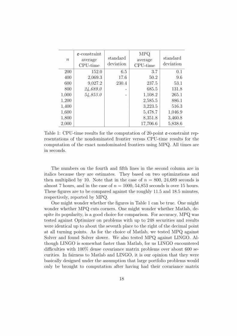
After coding the seven-step ε-constraint routine in Matlab, experimentswere conducted to compare CPU-times with MPQ. Results are in Table 1.The first column of the table specifies problem size in terms of the number ofsecurities n. For each of the non-italicized entries in the table, the sample sizewas 10 problems. Feasible region S in all problems was as in (10) with all αi =0 and all ωi = 1. In all problems, the Σ covariance matrices were 100% denseand were randomly generated using the method described in Hirschberger, Qiand Steuer [15]. To correspond to real covariance matrices, the diagonal andoff-diagonal elements had the same distributional characteristics as possessedby the real data alluded to in Table 3 of [15]. All experiments were conductedon a Dell 1.6GHz Centrino laptop with 1GB of RAM.

On the first line of the Table are the results for problems of size n = 200.Whereas it took Matlab on average 152 seconds to complete the 21 optimiza-tions required for a 20-point ε-constraint representation of a nondominatedfrontier, it took MPQ on average less than 4 seconds to compute an en-tire exact nondominated frontier. On the second line, with problems of sizen = 400, the numbers are 2,069 seconds and 50 seconds, respectively. Whatwe are observing is that, on average, MPQ takes less time to compute anentire exact nondominated frontier than it takes Matlab to compute just asingle point.

17

nε-constraint

averageCPU-time

standarddeviation

MPQaverage

CPU-time

standarddeviation

200 152.0 6.5 3.7 0.1400 2,069.3 17.6 50.2 9.6600 9,027.2 230.4 237.5 53.1800 24,689.0 - 685.5 131.8

1,000 54,853.0 - 1,108.2 265.11,200 2,585.5 886.11,400 3,223.5 516.31,600 5,478.7 1,046.91,800 8,351.8 3,460.82,000 17,706.6 5,838.6

Table 1: CPU-time results for the computation of 20-point ε-constraint rep-resentations of the nondominated frontier versus CPU-time results for thecomputation of the exact nondominated frontiers using MPQ. All times arein seconds.

The numbers on the fourth and fifth lines in the second column are initalics because they are estimates. They based on two optimizations andthen multiplied by 10. Note that in the case of n = 800, 24,689 seconds isalmost 7 hours, and in the case of n = 1000, 54,853 seconds is over 15 hours.These figures are to be compared against the roughly 11.5 and 18.5 minutes,respectively, reported by MPQ.

One might wonder whether the figures in Table 1 can be true. One mightwonder whether MPQ cuts corners. One might wonder whether Matlab, de-spite its popularity, is a good choice for comparison. For accuracy, MPQ wastested against Optimizer on problems with up to 248 securities and resultswere identical up to about the seventh place to the right of the decimal pointat all turning points. As for the choice of Matlab, we tested MPQ againstSolver and found Solver slower. We also tested MPQ against LINGO. Al-though LINGO is somewhat faster than Matlab, for us LINGO encountereddifficulties with 100% dense covariance matrix problems over about 600 se-curities. In fairness to Matlab and LINGO, it is our opinion that they werebasically designed under the assumption that large portfolio problems wouldonly be brought to computation after having had their covariance matrix

18

structures diagonalized. Unfortunately, diagonalizing a covariance matrixstructure is typically accompanied by a loss of information. Actually, CPU-times on the order of those reported by MPQ might be possible using the“fast algorithm” outlined in Markowitz, Todd, Xu and Yamane [28] on cer-tain problems. However, with that algorithm one must start with historicalobservations or scenarios, not a covariance matrix. MPQ has no such re-strictions. Anyway, a coded version of that algorithm is not known to beanywhere available. Thus with MPQ, we appear to get the best of severalworlds. Not only is it faster than anything avialable, it computes exactnondominated frontiers (as opposed to the approximations of the packages).Moreover, it can do so on dense covariance matrix problems that are largerthan anything that can be handled, as demonstrated, by either Matlab orLINGO.

As seen in Table 1, for the most difficult of mean-variance problems (i.e.,those with 100% dense covariance matrices), MPQ represents both a “better”and a “new” capability. For problems up to about 600-800 securities, it is abetter capability as it can typically compute an exact nondominated frontierin much less time than it takes Matlab to produce an approximation. Onproblems over about 800 securities, MPQ represents a new capability fordense covariance matrix problems as both Matlab and LINGO each run intotheir own difficulties while MPQ is still able to operate well within reasonabletime.

6 Multiple Criteria in Portfolio Selection

The mean-variance framework we have been discussing is summarized inFigure 4. With this figure as a reference point, the endeavor now is toexpand upon the framework with multiple objectives to provide a theoryof portfolio selection to meet the modeling needs of additional groups ofinvestors for which the assumptions of conventional mean-variance analysisoften fall short.

One such group of investors would consist of those who have the sameoverall focus as in the mean-variance theory we have been studying, exceptthat they do not buy into the assumption that all elements in µ and Σ canbe known with certainty at the beginning of the holding period. Investorsin this group might well wish to monitor their portfolios with other randomvariables such as dividends, growth in sales, and amount invested in R&D to

19

to onlymake money

?

overall focus

max{ rTx}s.t. x ∈ S

?

stochasticreflectionprogram

min{xTΣx }max{µTx}s.t. x ∈ S

equivalentdeterministic

implementationprogram

Figure 4: Hierarchical structure of the overall focus, stochastic reflection ofthe overall focus, and equivalent deterministic implementation of the stochas-tic reflection of conventional (mean-variance) portfolio selection.

hedge against errors that might be made when attempting to wrestle withinformation derived from inaccurate µ’s and Σ’s alone. Another group ofinvestors would consist of those who, in addition to end-of-holding-periodportfolio return, distinctly have other stochastic criteria, perhaps rangingfrom liquidity to social responsibility, that they would like to have simulta-neously maximized.

To articulate the concerns embedded in an investor’s more complex overallfocus, objectives such as from

max{dTx} dividends (13)

max{gTx} growth in sales

max{ aTx} amount invested in R&D

max{ sTx} social responsibility

max{ `Tx} liquidity

where d, g, a, s, ` ∈ Rn are random vectors, can be appended to portfolioreturn in the stochastic reflection program. Along with an equivalent de-terministic implementation of the (multiobjective) stochastic reflection pro-gram, we have Figure 5.

At the overall focus level in Figure 5, the intent is to build a portfo-

20

to build a multiplecriteria portfolio

?

overall focus

max{ rTx}...

s.t. x ∈ S

?

stochasticreflectionprogram

min{xTΣx }max{µTx}

...s.t. x ∈ S

equivalentdeterministic

implementationprogram

Figure 5: Hierarchical structure of the overall focus, stochastic reflection ofthe overall focus, and equivalent deterministic implementation of the stochas-tic reflection of multiple objective portfolio selection.

lio that achieves an investor’s optimal trade-off among various factors. Thethree vertical dots in the stochastic reflection program indicate the randomvariables in addition to portfolio return that are also to be optimized to thegreatest extent possible. In the equivalent deterministic implementation pro-gram, the vertical dots indicate the deterministic objectives that are utilizedto implement the objectives listed in the multiobjective stochastic reflectionprogram. While one could see the creation of a pair of expected value andvariance objectives for each stochastic objective, this does not always haveto be the case. As discussed in Caballero et al. [4], other alternatives exist.One such alternative is to simply implement a stochastic objective in theform of just its expected value. This could be appropriate with random vari-ables whose variance is much less or is not as important as others. One couldperhaps argue that most of the stochastic objectives listed in (13) could becandidates for such treatment.

21

7 Future Methods

With the potential of having one or more quadratic and two or more linearobjectives, equivalent deterministic implementation programs can becomedifficult. In fact, beyond the theoretical work of Guddat [10], there is littleto nothing in the literature about how to compute the nondominated setsof such problems. However, in the case of one quadratic and two linear ob-jectives, progress is being made in Hirschberger, Qi and Steuer [14] and onthis we comment. With an understanding of nondominated sets in the one-quadratic-one-linear and one-quadratic-two-linear situations, one should bein a position to perceive the nature of nondominated sets in one-quadratic-three-or-more-linear situations. While the protocol of first computing thenondominated set and then selecting from it a most preferred solution re-mains the same, the mechanics of carrying out these tasks involve a signifi-cant step up in difficulty.

With three or more objectives, the nondominated set is no longer, inthe parlance of mean-variance optimization, a frontier, but it is now a sur-face. Consider a one-quadratic-two-linear case. Instead in being piecewiseparabolic in R2, the nondominated set is now platelet-wise paraboloidic inR3 (like tiles on the front of a space shuttle) as in Figure 6. Fortunately,with some extra coding, the algorithm programmed into MPQ allows for ageneralization to one quadratic and multiple linear objectives. We are notaware of any other research, either published or in progress, that can com-pute the exact nondominated sets of such problems. In computing an exactnondominated set, what MPQ is able to output includes: (1) the equation ofthe paraboloid that each nondominated platelet is a part of, (2) the cornerpoints (as indicated by z1 to z4 in Figure 6) of each nondominated plateletin criterion space, and (3) the extreme points (not shown) of the polyhe-dron subset of efficient points in S that corresponds to each nondominatedplatelet. That is, the set of all images of points in an efficient polyhedronsubset constitutes a nondominated platelet on the surface of Z, and the set ofall inverse images of points on a nondominated platelet constitute an efficientpolyhedron subset within or on the surface of S.

Preliminary computational experience with MPQ on computing the non-dominated sets of portfolio problems with the same characteristics as in Table1, but with an extra linear objective, are given in Table 2. For example, witha sample size of 10, problems of size n = 300 had on average almost 2,132platelets and took on average 23.5 seconds to compute. More extensive re-

22

Expecte

d R

etu

rn

Standard Deviation

z1

z3

z2

z2

2nd Linear

Figure 6: A portrayal of the platelet-wise nature of a nondominated surfaceof a one-quadratic-two-linear problem, with the corner points of the shadedplatelet as indicated.

sults will be reported in the future.

nnumber

ofplatelets

standarddeviation

MPQaverage

CPU-time

standarddeviation

100 1,131.2 414.6 0.8 0.1200 1,815.0 249.2 4.9 0.7300 2,131.6 599.9 23.5 7.0400 2,117.8 637.8 65.9 28.6

Table 2: Results for the computation of all platelets of the nondominatedsets of one-quadratic-two-linear portfolio problems using MPQ. Times are inseconds.

With regard to the searching of a nondominated set of a problem such asin Table 2, one strategy is to discretize the nondominated set to some desireddegree of resolution. This can be accomplished platelet by platelet as follows.For a given platelet, take convex combinations of the extreme points of itspolyhedron subset in S. Because platelet size tends to increase the moredistant a platelet is away from the point in Z that minimizes the quadraticobjective, one would probably want to increase the number of convex combi-nations the further a platelet is away. Then with perhaps thousands, tens ofthousands, or hundreds of thousands of points, the question is how to iden-

23

tify a most preferred one. Four strategies come to mind. One is to employmultiple probing as in the variant of the Tchebycheff Method described inSteuer, Silverman and Whisman [39]. Another is to pursue a projected linesearch strategy as advanced in Korhonen and Karaivanova [19]. A third isto utilize a criterion vector component classification scheme as, for instance,in Miettinen [31]. And a fourth might involve the utilization of some of thevisualization techniques from Lotov, Bushenkov and Kamenev in [21].

8 Conclusions

The capabilities of MPQ provide not only a new capability for mean-varianceportfolio optimization but a new world of possibilities with regard to themodeling and solution of multiple objective portfolio selection formulations.As discussed in Section 1, codes for solving for exact nondominated frontiersare generally not known to be available, either in public domain form orwithin the context of popular commercial packages, for problems with morethan 248 securities. Furthermore, as shown in the leftmost two columns ofTable 1, it is basically not possible using software such as Matlab to computeeven approximations of the nondominated frontier in problems with densecovariance matrices beyond about 800 securities in reasonable time (say 4hours). However, as shown in the rightmost two columns of Table 1, MPQ cancompute exact nondominated frontiers of dense covariance matrix problemswith up to near 2,000 securities in reasonable time.

In addition, as shown in Table 2, MPQ is able to compute exact nondom-inated frontiers of tri-criterion dense covariance matrix formulations with upto at least 400 securities in reasonable time. This opens up a whole new worldof modeling possibilities, and with the importation of methods from multiplecriteria optimization, new areas of portfolio optimization that weren’t evenworth contemplating because of the futility of the solution situation beforecan now be brought to the forefront.

References

[1] B. Aouni, F. Ben Abdelaziz, and R. El-Fayedh. Chance constrainedcompromise programming for portfolio selection. Laboratoire LARO-

24

DEC, Institut Superieur de Gestion, La Bardo 2000, Tunis, Tunisia,2005.

[2] M. Arenas Parra, A. Bilbao Terol, and M. V. Rodrıguez Urıa. A fuzzygoal programming approach to portfolio selection. European Journal ofOperational Research, 133(2):287–297, 2001.

[3] C. A. Bana e Costa and J. O. Soares. A multicriteria model for portfoliomanagement. European Journal of Finance, 10(3), 2004. 198-211.

[4] R. Caballero, E. Cerda, M. M. Munoz, L. Rey, and I. M. Stancu-Minasian. Efficient solution concepts and their relations in stochasticmultiobjective programming. Journal of Optimization Theory and Ap-plications, 110(1):53–74, 2001.

[5] J. Y. Campbell, A. W. Lo., and A. C. Mackinlay. The Econometrics ofFinancial Markets. Princeton University Press, Princeton, New Jersey,1997.

[6] Cplex. “Cplex 9.1 User’s Manual,” ILOG, Inc., Mountain View, Cali-fornia, 2005.

[7] M. Ehrgott, K. Klamroth, and C. Schwehm. An MCDM approachto portfolio optimization. European Journal of Operational Research,155(3):752–770, 2004.

[8] E. J. Elton, M. J. Gruber, S. J. Brown, and W. Goetzmann. ModernPortfolio Theory and Investment Analysis. John Wiley, New York, 6thedition, 2002.

[9] M. Erhgott. Multicriteria Optimization. Springer, Berlin, 2nd edition,2005.

[10] J. Guddat. Stability in convex quadratic programming. Operations-forschung und Statistik, 7:223–245, 1976.

[11] J. B. Guerard and A. Mark. The optimization of efficient portfolios:The case for an R&D quadratic term. Research in Finance, 20:217–247,2003.

25

[12] W. G. Hallerbach and J. Spronk. A multidimensional framework forfinancial-economic decisions. Journal of Multi-Criteria Decision Analy-sis, 11(3):111–124, 2002.

[13] M. Hirschberger, Y. Qi, and R. E. Steuer. Quadratic parametric pro-gramming for portfolio selection with random problem generation andcomputational experience. In-preparation working paper, Departmentof Banking and Finance, University of Georgia, Athens, 2006.

[14] M. Hirschberger, Y. Qi, and R. E. Steuer. Tri-criterion quadratic-linearprogramming. In-preparation working paper, Department of Bankingand Finance, University of Georgia, Athens, 2006.

[15] M. Hirschberger, Y. Qi, and R. E. Steuer. Randomly generatingportfolio-selection covariance matrices with specified distributional char-acteristics. European Journal of Operational Research, 2006. forthcom-ing.

[16] C. F. Huang and Litzenberger R. H. Foundations for Financial Eco-nomics. Prentice-Hall, Englewood Cliffs, New Jersey, 1988.

[17] J. E. Ingersoll. Theory of Financial Decision Making. Rowman & Lit-tlefield, 1987.

[18] C. P. Jones. Investments: Analysis and Management. John Wiley &Sons, New York, 7th edition, 2000.

[19] P. Korhonen and J. Karaivanova. An algoithm for projecting a referencedirection onto the nondominated set of given points. IEEE Transactionson Systems, Man, and Cybernetics, 29(5):429–435, 1999.

[20] A. W. Lo, C. Petrov, and M. Wierzbicki. It’s 11pm – Do you knowwhere your liquidity is? The mean-variance-liquidity frontier. Journalof Investment Management, 1(1):55–93, 2003.

[21] A. B. Lotov, V. A. Bushenkov, and G. K. Kamenev. Interactuve DecisionMaps: Approximation and Visualization of Pareto Frontier. KluwerAcademic Publishers, Boston, 2004.

[22] D. G. Luenberger. Investment Science. Oxford University Press, NewYork, 1997.

26

[23] SAS Institute Inc. Stock Market Analysis Using the SAS System: Port-folio Selection and Evaluation, Cary, North Carolima, 1994.

[24] H. M. Markowitz. Portfolio selection. Journal of Finance, 7(1):77–91,1952.

[25] H. M. Markowitz. The optimization of a quadratic function subject tolinear constraints. Naval Research Logistics Quarterly, 3:111–133, 1956.

[26] H. M. Markowitz and A. Perold. Portfolio analysis with factors andscenarios. Journal of Finance, 36(14):871–877, 1981.

[27] H. M. Markowitz and G. P. Todd. Mean-Variance Analysis in PortfolioChoice and Capital Markets. Frank J. Fabozzi Associates, New Hope,Pennsylvania, 2000.

[28] H. M. Markowitz, P. Todd, G. Xu, and Y. Yamane. Fast computationof mean-variance efficient sets using historical covariances. Journal ofFinancial Engineering, 1(2):117–132, 1992.

[29] Matlab. Optimization Toolbox for Use with Matlab, Version 7.0.1 (R14),Mathworks, Inc., Natick, Massachusetts, 2004.

[30] H. P. Mayo. Investments: An Introduction. Harcourt, Fort Worth,Texas, 6th edition, 2000.

[31] K. M. Miettinen. Nonlinear Multiobjective Optimization. Kluwer,Boston, 1999.

[32] W. Ogryczak. Multiple criteria linear programming model for portfolioselection. Annals of Operations Research, 97:143–162, 2000.

[33] R. Roll. A critique of the asset pricing theory’s tests. Journal of Finan-cial Economics, 4:129–176, 1977.

[34] T. L. Saaty. Decision Making for Leaders. RWS Publications, Pitts-burgh, 1999–2000 edition, 1999.

[35] L. Schrage. Optimization Modeling with LINGO. Lindo Publishing,Chicago, 2003.

[36] L. Schrage. LINGO User’s Guide. Lindo Publishing, Chicago, 2004.

27

[37] R. E. Steuer. Multiple Criteria Optimization: Theory, Computation andApplication. John Wiley, New York, 1986.

[38] R. E. Steuer, Y. Qi, and M. Hirschberger. Multiple objectives in portfolioselection. Journal of Financial Decision Making, 1(1):11–26, 2005.

[39] R. E. Steuer, J. Silverman, and A. W. Whisman. A combined Tcheby-cheff/aspiration criterion vector interactive multiobjective programmingprocedure. Management Science, 39(10):1255–1260, 1993.

[40] Frontline Systems. “Premium Solver Platform 6.5,” Incline Village,Nevada, 2005.

[41] S. Wolfram. The Mathematica Book. Wolfram Media, 5th edition, 2003.

[42] C. Zopounidis and M. Doumpos. INVESTOR: A decision support sys-tem based on multiple criteria for portfolio selection and composition.In A. Colorni, M. Paruccini, and B. Roy, editors, A-MCD-A Aide MultiCritere a la Decision - Multiple Criteria Decision Aiding, pages 371–381.European Commission Joint Research Centre, Brussels, 2000.

28

Summary

This paper addresses the problem of portfolio selection in finance. In manycases, currently available software to compute the efficient frontier runs intodifficulty in problems with more than about 600 securities. To proceed be-yond this size, it is often necessary to modify the problem in which casethere is typically a loss of information. In this paper, we discuss a computercapability that can exactly compute mean-variance efficient frontiers of prob-lems with up to 2,000 securities in very reasonable time (even if a problem’scovariance matrix is 100% dense).

The paper also discusses an augmentation to the theory of portfolio se-lection that allows multiple objectives (such as dividends, liquidity, socialresponsibility, amount invested in R&D, and so forth) to be incorporatedinto the portfolio selection process. In such problems, the efficient set is nolonger a “frontier,” but is now best described as a “surface” with the inter-esting property that it is composed of platelets (like on the back of a turtle).Moreover, the computer capability that can extend exact computations ofmean-variance efficient frontiers out to 2,000 securities also has, after addi-tional coding, the ability to exactly compute all of the platelets of multipleobjective efficient surfaces of problems with up to about 400 securities.

29