portfolio management using structured products - kth · pdf fileportfolio management using...
TRANSCRIPT

Royal Institute of Technology
Master’s Thesis
Portfolio management using structuredproducts
The capital guarantee puzzle
Markus [email protected]
Stockholm, January 2011


Abstract
The thesis evaluates the concept of a structured products fund and investigates how a fund basedon structured products should be constructed to be as competitive as possible. The focus lieson minimizing the risk of the fund and on capital guarantee. The difficulty with this type ofallocation problem is that the available products mature before the investment horizon, thusthe problem of how the capital should be reinvested arises. The thesis covers everything fromnaive fund constructions to more sophisticated portfolio optimization frameworks and results inrecommendations regarding how a portfolio manager should allocate its portfolio given differentsettings. The study compares different fund alternatives and evaluates them against, competing,benchmark funds.
The thesis proposes a framework called the modified Korn and Zeytun framework whichallocates a portfolio based on structured products, which have maturity prior to the end of theinvestment horizon, in optimal CVaR sense (i.e. appropriate for funds).
The study indicates that the most important concept of a structured products fund is trans-action costs. A structured products fund cannot compete against e.g. mixed funds on the marketif it cannot limit its transaction costs at approximately the same level as competing funds. Theresults indicate that it is possible to construct a fund based on structured products that is com-petitive and attractive given low commission and transaction costs.
Keywords: Structured products fund, structured products, portfolio theory, portfolio optimiza-tion, portfolio management, Conditional Value-at-Risk, transaction costs


Acknowledgements
I would like to thank my supervisor at KTH Mathematical Statistics, Filip Lindskog, for greatfeedback and guidance as well as my supervisors at Nordea Markets, Karl Lindqvist and WilliamSjöberg, for essential knowledge in the field of structured products, feedback and ideas.
Stockholm, January 2011
Markus Hveem
v


Table of Contents
1 Introduction 11.1 Market risk . . . . . . . . . . . . . . . . . . . . . . . . . . . . . . . . . . . . . . . 11.2 Capital guarantee . . . . . . . . . . . . . . . . . . . . . . . . . . . . . . . . . . . . 11.3 Purpose . . . . . . . . . . . . . . . . . . . . . . . . . . . . . . . . . . . . . . . . . 21.4 Outline . . . . . . . . . . . . . . . . . . . . . . . . . . . . . . . . . . . . . . . . . 3
2 Theoretical Background 52.1 Risk measures . . . . . . . . . . . . . . . . . . . . . . . . . . . . . . . . . . . . . . 5
2.1.1 Absolute lower bound . . . . . . . . . . . . . . . . . . . . . . . . . . . . . 52.1.2 Value-at-Risk . . . . . . . . . . . . . . . . . . . . . . . . . . . . . . . . . . 62.1.3 Conditional Value-at-Risk . . . . . . . . . . . . . . . . . . . . . . . . . . . 7
2.2 Principal component analysis . . . . . . . . . . . . . . . . . . . . . . . . . . . . . 72.3 Scenario based optimization . . . . . . . . . . . . . . . . . . . . . . . . . . . . . . 9
2.3.1 Conditional Value-at-Risk . . . . . . . . . . . . . . . . . . . . . . . . . . . 102.3.2 Minimum regret . . . . . . . . . . . . . . . . . . . . . . . . . . . . . . . . 10
2.4 Transaction costs . . . . . . . . . . . . . . . . . . . . . . . . . . . . . . . . . . . . 11
3 Financial Assets 153.1 Definition of a structured product . . . . . . . . . . . . . . . . . . . . . . . . . . 15
3.1.1 Dynamics . . . . . . . . . . . . . . . . . . . . . . . . . . . . . . . . . . . . 163.2 Zero-coupon bond . . . . . . . . . . . . . . . . . . . . . . . . . . . . . . . . . . . 173.3 Plain vanilla call option . . . . . . . . . . . . . . . . . . . . . . . . . . . . . . . . 17
3.3.1 A note regarding the critique against B & S . . . . . . . . . . . . . . . . . 18
4 The Capital Protection Property 194.1 Capital guarantee . . . . . . . . . . . . . . . . . . . . . . . . . . . . . . . . . . . . 194.2 Naive fund constructions . . . . . . . . . . . . . . . . . . . . . . . . . . . . . . . . 20
4.2.1 Naive fund construction number 1 . . . . . . . . . . . . . . . . . . . . . . 204.2.2 Naive fund construction number 2 . . . . . . . . . . . . . . . . . . . . . . 254.2.3 Analysis and summary . . . . . . . . . . . . . . . . . . . . . . . . . . . . . 294.2.4 Prevalent risk factors . . . . . . . . . . . . . . . . . . . . . . . . . . . . . . 29
4.3 Investigation of the option portfolio . . . . . . . . . . . . . . . . . . . . . . . . . 314.3.1 Portfolio construction and modeling . . . . . . . . . . . . . . . . . . . . . 314.3.2 Portfolios and results . . . . . . . . . . . . . . . . . . . . . . . . . . . . . . 324.3.3 Analysis and implications . . . . . . . . . . . . . . . . . . . . . . . . . . . 35
4.4 Comparison with competition . . . . . . . . . . . . . . . . . . . . . . . . . . . . . 364.4.1 Client base . . . . . . . . . . . . . . . . . . . . . . . . . . . . . . . . . . . 374.4.2 Benchmark fund . . . . . . . . . . . . . . . . . . . . . . . . . . . . . . . . 374.4.3 Structured products fund 1 . . . . . . . . . . . . . . . . . . . . . . . . . . 374.4.4 Scenarios . . . . . . . . . . . . . . . . . . . . . . . . . . . . . . . . . . . . 394.4.5 Results, structured products fund vs benchmark . . . . . . . . . . . . . . 394.4.6 Analysis and summary . . . . . . . . . . . . . . . . . . . . . . . . . . . . . 424.4.7 Additional stress test . . . . . . . . . . . . . . . . . . . . . . . . . . . . . . 444.4.8 Backtesting . . . . . . . . . . . . . . . . . . . . . . . . . . . . . . . . . . . 45
vii

4.4.9 Structured products fund 2 . . . . . . . . . . . . . . . . . . . . . . . . . . 474.5 Alternative definitions of capital protection . . . . . . . . . . . . . . . . . . . . . 51
4.5.1 Definition 1 - Absolute lower bound . . . . . . . . . . . . . . . . . . . . . 514.5.2 Definition 2 - CVaR . . . . . . . . . . . . . . . . . . . . . . . . . . . . . . 52
5 Modeling Financial Assets 535.1 Volatility and option pricing . . . . . . . . . . . . . . . . . . . . . . . . . . . . . . 535.2 Index . . . . . . . . . . . . . . . . . . . . . . . . . . . . . . . . . . . . . . . . . . 535.3 Yield curve . . . . . . . . . . . . . . . . . . . . . . . . . . . . . . . . . . . . . . . 545.4 A PCA model for the yield curve and index . . . . . . . . . . . . . . . . . . . . . 54
5.4.1 Data set . . . . . . . . . . . . . . . . . . . . . . . . . . . . . . . . . . . . . 555.4.2 PCA results . . . . . . . . . . . . . . . . . . . . . . . . . . . . . . . . . . . 555.4.3 Historical simulation . . . . . . . . . . . . . . . . . . . . . . . . . . . . . . 565.4.4 Monte Carlo simulation . . . . . . . . . . . . . . . . . . . . . . . . . . . . 58
6 Portfolio Optimization 656.1 Fixed portfolio weights . . . . . . . . . . . . . . . . . . . . . . . . . . . . . . . . . 656.2 Rolling portfolio weights . . . . . . . . . . . . . . . . . . . . . . . . . . . . . . . . 696.3 Benchmark fund . . . . . . . . . . . . . . . . . . . . . . . . . . . . . . . . . . . . 716.4 Dynamic portfolio weights . . . . . . . . . . . . . . . . . . . . . . . . . . . . . . . 72
6.4.1 Modifying the Korn and Zeytun framework . . . . . . . . . . . . . . . . . 736.4.2 Dependence of the initial yield curve . . . . . . . . . . . . . . . . . . . . . 756.4.3 Observed paths . . . . . . . . . . . . . . . . . . . . . . . . . . . . . . . . . 76
6.5 Transaction costs . . . . . . . . . . . . . . . . . . . . . . . . . . . . . . . . . . . . 786.6 Summary . . . . . . . . . . . . . . . . . . . . . . . . . . . . . . . . . . . . . . . . 806.7 Backtesting . . . . . . . . . . . . . . . . . . . . . . . . . . . . . . . . . . . . . . . 81
7 Conclusions 83
Bibliography 85
Appendices 91
A Naive fund constructions - Additional scenarios 91
B Option portfolios - Additional portfolios 93
C SPF vs Benchmark - Additional scenarios 95
D Correlations between the market index and the yield curve 99
E Optimization problem - Arbitrary start yield curve 101
M. Hveem viii (103)

CHAPTER 1Introduction
Structured products are a structured form of investment vehicles that consists of a bond anda market exposed financial instrument. The popularity of investing in Equity-Linked Notes,and other structured products, has been significant exceeding 55.1 billion SEK in Sweden aloneduring 2009 (My News Desk, 2010, [32]). One reason for their popularity is that they possessthe property of capital guarantee. Thus many investors have a belief that these products are safeand do not realize the impact of credit risk. An investor can by investing in structured productsparticipate in the market besides the capital guaranteed part (the bond). Thus investors areprotected in bear markets and participate in bull markets.
The other major risk for an investor is market risk; the key to avoid market risk is bydiversifying. Market risk imposes a demand for applying a diversification framework, similarto the one of Markowitz’s (1952, [30]) seminal work on basic portfolio management theory,applicable to structured products. Most studies in the area have been conducted by using astructured product, a bond, the underlying and an option on the underlying as the investmentuniverse in a one period model (as in Martellini et al. (2005, [31])), which is inadequate to describethe investment universe for e.g. a hedge fund. The first study conducted on the subject, using alonger investment horizon than the time to maturity for the structured product, was performedby Korn and Zeytun (2009, [27]). This setup is more relevant for an investor that must rebalanceits portfolio at different intermediate time points, and especially when the investor is allowed toinvest in more than just one structured product.
1.1 Market risk
It has been shown in studies of the Swedish market for structured products that an investor usingstructured products in a diversified portfolio can achieve a fair return during bull markets andtake advantage of the capital protection property (to some extent) of the structured products inthe bear markets (Hansen and Lärfars, 2010, [19]; Johansson and Lingnardz, 2010, [25]).
These studies indicate that there are advantages of diversification when investing in structuredproducts against market risk. Many investors on the Swedish market of structured products aresmall private investors and thus not willing to commit most of their capital in one investmentcategory (Shefrin, 2002, [35]). Hence to offer the advantages of diversification in structuredproducts to small investors the concept of a fund based on structured products emerges. Bycreating a fund based on structured products it is possible to decrease the required amountinvested for each individual investor and practically gain the same advantages as if the investorhad the possession itself.
1.2 Capital guarantee
The concept of market risk and diversifying using a set of numerous assets is very appealing to aninvestor, especially if the investment is capital guaranteed. The main issue is that the portfoliobased on several structured products with different maturities will not be capital guaranteed.
1

Chapter 1. Introduction
When, in the setting of structured products, a product is capital guaranteed it means thatthe investor will at least receive the invested amount, at maturity (when disregarding the impactof defaults). In the setting of a fund the investment horizons will instead be overlapping andof approximately one to five years, thus the capital guarantee should be measured during eachof these investment periods. Problem arises when the fund holds positions in products withmaturity beyond the investment horizon, since all structured products can have a value of zerobefore maturity due to changes in interest, movement of the underlying etc. Also if products havematurity prior to the investment horizon’s end the issue of how the payoff should be reinvestedarises. Consider that the fund should not only be guaranteed during one investment horizon,but several, each new investor wants to have the property of capital guarantee over its owninvestment horizon. Thus if the fund should be capital guaranteed for each investor, with aninvestment horizon of τi years, the return of the portfolio of every single τi year long time periodshould be positive. It is obvious that it is difficult to gain the property of capital guarantee incombination with the possibility of a high return.
0 5 10 15 20 250
20
40
60
80
100
120
X: 24Y: 92.84
Quarter
$
Price Underlying
NAV FundStart of investment
Figure 1.1: The underlying has 1% in return each quarter until quarter 12, when the investor buysa share of the fund, after quarter 12 the underlying has −5% in return quarterly, σ =0.15, r = 0.015 p.q., hence the fund is not capital guaranteed.
The example in Figure 1.1 illustrates the value of a fund that consists of rolling capitalguaranteed Equity-Linked Notes (notional amount of the bond equals to the price of the product)each quarter with a maturity of three years. Thus each product is capital guaranteed but thefund is not capital guaranteed over the three-year time horizon. The investor in this example isan investor with an investment horizon of three years and holds only capital guaranteed products(a total of 23 products, 12 at a time) with a maximum time to maturity of three years. Duringthis time period the fund value decreases with 7.16%, hence the simple naive fund constructionis not capital protected.
As the price of the underlying goes up the value of the fund increases since the options gainmore in value. This implies that after twelve quarters, when the underlying has gone up a totalof 12.68%, the fund’s NAV consists of options in a high extent, which makes the investment morerisky and erasing the capital guarantee.
1.3 Purpose
The purpose of this thesis is to investigate if it is possible to construct a portfolio based onstructured products that possesses the property of capital protection. The focus lies on developingan alternative definition of capital protection, since there obviously does not exist any structuredproducts fund (SPF) fulfilling the requirements of absolute capital guarantee. The objective is
M. Hveem 2 (103)

1.4. Outline
also to investigate how a fund with as low downside risk as possible, with a decent expectedreturn (should be competitive in relation to competing funds), should be constructed. Theinvestigation is performed numerically based on simulating trajectories of future price patternsfor available structured products and by solving an optimization problem allocating the portfoliobased on CVaR constraints as in Uryasev (2000, [38]). Since the thesis will only consider investingin products with the same underlying the importance of using a scheme based on Black andLitterman’s (1992) studies in [8] is reduced, thus exploring the impact of active subjective viewson the investment choice is left for future research, as well as the possibility of multiple underlying.
The thesis focuses on market associated risks and will not evaluate the impact of credit riskon the portfolio choice. Thus when investigating if the products are capital protected the impactof defaults is neglected, this is usually how the terminology capital protection is used in theconcept of structured products.
1.4 Outline
Chapter 2 covers the most fundamental basics which the thesis has its foundation in, such as thetheory of risk measures, scenario based optimization and principal component analysis. It is notnecessary for the reader to go through this chapter, since it is not imperative to understand thesetheories to understand the result. In Chapter 3 the definition of a structured product is coveredand how the individual components are priced. Chapter 4 covers the issue of capital guarantee,the definition of capital guarantee, how the portfolio should be allocated initially to attain ashigh degree of capital protection as possible. The chapter covers everything from naive fundconstructions to benchmarking with potential competition. A scheme to minimize the downsiderisk is also described in the chapter.
Chapter 5 covers how the financial assets are modeled and discloses the details regarding thePCA. Chapter 6 covers three proposed allocation schemes, where a modified Korn and Zeytunframework is recommended. In the last chapter conclusions are drawn regarding the results andrecommendations for future studies are given.
M. Hveem 3 (103)


CHAPTER 2Theoretical Background
This chapter covers the theoretical background that the reader should be familiar with to under-stand how the study is conducted. By understanding the concepts in this chapter it is also easierto understand how to replicate the results and also the assumptions affecting the results. Thechapter will cover everything from risk measures and principal component analysis (which is anintegral part of the modeling) to scenario based optimization and transaction costs. Notable, itis not necessary to understand the concepts discussed in this chapter to understand the resultsof the study.
To ensure full clarity for the reader matrices are written as bold upper case characters, vectorsas bold lower case characters and transposed with superscript T, not only in this chapter butalso throughout the whole paper.
2.1 Risk measures
The concept of risk has been around finance for more than fifty years. Markowitz introducedhis seminal work within portfolio theory during 1952 [30] where he used standard deviation(volatility) as risk measure to find the optimal tradeoff between risk and return. Since thenit has been shown that assets’ log returns are not multivariate normal distributed and that thedistribution of stock returns often exhibit negative skewed kurtosis (Fisher, 1999, [14]), especiallyaround extreme events such as the 1987 stock market crash, the Black Monday 19th Octoberwhen the Dow Jones Industrial Average dropped by 508 points to 1738.74, a 22.61% decrease(Browning, 2007, [11]). Such extreme events prove that measuring risk with the variance is notadequate, not even for stock returns.
A portfolio containing derivatives is not, in general, symmetric and variance (even if stockreturns are relative symmetric) is thus not an adequate risk measure. Some risk measures havebeen introduced to capture these heavy tailed, skewed distributions such as Value-at-Risk (VaR),Conditional-Value-at-Risk (CVaR, closely related to Expected Shortfall) (Acerbi, 2002, [3]). An-other risk measure, which is not as commonly used as VaR and CVaR is the absolute lowerbound, which measures the worst-case outcome.
Further the net worth of the fund portfolio at time T is denoted as X = XT −Xt, where Xt
is the value of the portfolio at time t.
2.1.1 Absolute lower boundAn acceptable portfolio is a portfolio which final net worths are those that are guaranteed toexceed a certain fixed number (e.g. a percentage of the initial investment) c, i.e. the set ofacceptable portfolios must fulfill these requirements,
A = {X ∈ X : X ≥ c} ,
which gives the risk measure,
ρ (X ) = min {m : m (1 + rf ) + X ∈ A} = min {m : m (1 + rf ) + X ≥ c} .
5

Chapter 2. Theoretical Background
x0 = x0 (X ) is denoted as the smallest value that X can take, notice that,
ρ (X ) = min {m : m (1 + rf ) + X ≥ c} =c− x0
1 + rf.
Thus the definition is regarding the worst possible outcome of the position at time T . Whenregarding absolute capital guarantee the portfolio satisfies ρ (X ) ≤ 0 (Hult and Lindskog, 2009,[23]).
2.1.2 Value-at-Risk
Value-at-Risk (VaR) is one of the most important concepts within risk management and is alsoregulated by the FSA in many countries and by the guidelines from the second Basel Accordregarding minimum capital requirements (BIS, 2006, [5]). The idea of VaR is that VaRα (Lw) isthe value that the portfolio’s loss will be less than or equal to with a probability of α. Thus VaRis given as (a similar notation is given in [27]),
• Let Lw denote the loss of the portfolio with the portfolio weights w, and the probability ofLw not exceeding a threshold m as,
ψ (w,m) = P (Lw ≤ m) .
• Then Value-at-Risk VaRα (Lw) is defined as the loss with a confidence level of α ∈ [0, 1]by,
VaRα (Lw) = min {m ∈ R : ψ (w,m) ≥ α} ,
or,
VaRα (Lw) = min {m ∈ R : P (Lw ≤ m) ≥ α} .
• Where Lw = −Rw, where Rw is the return associated with the portfolio vector w, and thereturn is defined as,
Rw =final wealthinitial wealth
− 1.
There exists several areas of critique against VaR; one of the most common critiques is that itis not a coherent risk measure (Hult and Lindskog, 2009, [23]). Also it is not very useful fordistributions that have heavy tails, since it only measures the outcomes at the quantile α. Manyblame Value-at-Risk of being an integral part why a financial system may fail, since the modelunderestimates the risk/implication of market crashes (Brooks and Persand, 2000, [10]) anddoes not take into account the size of the losses exceeding VaR, thus traders have the possibilityto hide risk in the tail. Also, VaR is a non-convex and non-smooth function which in manycases has multiple local maximums and minimums, thus it is very hard to construct a portfoliooptimization scheme which is effective enough to still be robust and give valid results (Uryasev,2000, [38]).
Instead of VaR many authors propose Conditional Value-at-Risk (CVaR), which is mucheasier to implement in portfolio optimization as proposed by Uryasev et al. in [28, 33, 38]. AlsoAlexander et al. (2006, [4]) have recently developed an optimization scheme which is very efficientfor minimizing CVaR and VaR for portfolios of derivatives, but it is much more complex thanthe one proposed by Uryasev et al., and Alexander et al.’s theory will not be covered in thispaper.
M. Hveem 6 (103)

2.2. Principal component analysis
2.1.3 Conditional Value-at-Risk
CVaR is based on the definition of VaR since it is the expected loss under the condition that theloss exceeds or equals the VaR, i.e. it is defined as,
CVaRα (Lw) = E [Lw | Lw ≥ VaRα (Lw)] .
CVaR is a coherent risk measure and more adequate than VaR since it discloses the expectationof the loss if the loss exceeds the VaR, which is an important concept in risk management.The goal of portfolio optimization is often to maximize the return subject to a demand on themaximum risk acceptable. The optimization problem reduces to a linear optimization problemwith linear constraints, in the CVaR case. The advantage with a linear optimization problem isthat it can be solved using the simplex method.
Krokhmal et al. (2002, [28]) have shown that the solutions to the optimization problems,
minx∈X−R (x) , s.t. CVaRα (Lw) ≤ C, (2.1)
and,minx∈X−R (x) , s.t. Fα (w, β) ≤ C, (2.2)
give the same minimum value where,
Fα (w, β) = β +1
1− α
∫y∈Rm
[L (w, y)− β]+p (y) dy,
CVaRα (Lw) = minβ∈R
Fα (w, β) ,
and L (w, y) is the loss function associated with the portfolio vector w, y ∈ Rm is the set ofuncertainties which determine the loss function. If the CVaR constraint in 2.1 is active, then(w∗, β∗) minimizes 2.2 if and only if w∗ minimizes 2.1 and β∗ ∈ arg minβ∈R Fα (w, β). Whenβ∗ ∈ arg minβ∈R Fα (w, β) reduces to a single point, then β∗ gives the corresponding VaR withconfidence level of α (Korn and Zeytun, 2009, [27]). Thus it is possible to solve the optimizationproblem 2.2 instead, which is easily transformed to a linear optimization problem (disclosedin Section 2.3), since it generates the same solution as 2.1, for the proof and more detailedinformation please consult [28, 33, 38].
2.2 Principal component analysis
Principal component analysis (PCA) is a common tool to generate scenarios for changes inthe yield curve and returns for other types of assets. The idea of PCA is that data sets ofintercorrelated quantities can be separated into orthogonal variables, which explains the varianceand dependence in the data in a simpler way. Thus the number of factors to simulate can bereduced drastically by reducing the number of risk factors to model. A whole yield curve can oftenbe reduced into only three factors, or so-called principal components, thus PCA is a useful tool togenerate scenarios that are parsimonious. Studies have shown that by using principal componentanalysis only two or three principal components are often enough to describe more than 95% ofthe variation in a yield curve (Barber and Copper, 2010, [6]; Litterman and Scheinkman, 1991,[29]). The main idea is to transform the data to a new orthogonal coordinate system such thatthe greatest variance by any projection of data comes to lie on the first coordinate (i.e. firstprincipal component), the second greatest variance by any projection on the second coordinateand so on.
M. Hveem 7 (103)

Chapter 2. Theoretical Background
Consider a setting with m assets, n number of observations and that the asset returns aregiven as a n×m matrix denoted R̃. It is important to center the returns/data by subtracting itsmean to perform the PCA and also normalize the data by dividing with
√(n− 1) (or by
√n).
Let denote R = R̃−µ√n−1 , this type of PCA is referred to as covariance PCA since the matrix RTR
is a covariance matrix (the covariance matrix of the returns). It is also common with correlationPCA, in which each variable is divided by its norm, making RTR a correlation matrix (mostcommon in statistical packages such as MATLAB and R), correlation PCA will be used in thisthesis (Abdi, 2010, [2]).
By using singular value decomposition R can be written on the following form,
R = P∆QT,
where P is a n×n orthonormal matrix, Q is a m×m orthonormal matrix (called loading matrixand each column corresponds to one PC) and ∆ is a n × m matrix with non-negative valueson the diagonal. The PCA creates new variables called principal components, which are linearcombinations of the original variables and are defined in a way such that the amount of variationassociated with them are in decreasing order and orthogonal to each other. Let denote the factorscores F (observations of the principal components) as,
F = P∆,
thus,F = P∆ = P∆QTQ = RQ,
which implies that the ith observation of the jth original variable is expressed as follows,
ri,j = QT1,jFi,1 + ...+ QT
m,jFi,m.
Next RTR, is investigated,
RTR =(P∆QT)T P∆QT = Q∆TPTP∆QT = Q∆T∆QT = Q∆2QT.
∆ is a diagonal matrix and ∆2 equals the diagonal matrix Λ containing the (positive) eigenvaluesλ1, ..., λn to RTR (since RTR is a positive semi-definite matrix), Q is an orthogonal matrix.An orthogonal matrix has the property QT = Q−1, thus QTQ = QQT = I. The columns inQ, q1, ...qm are the corresponding eigenvectors of RTR, which are orthonormal. It is possibleto assume, without loss of generality, that the columns of Λ and Q are ordered such that thediagonal elements in Λ appear in descending order. Note that,
Cov(FT) = E
[QTRTRQ
]= QTCov (R) Q = QTRTRQ = Λ,
thus the components of F are uncorrelated and have variances λ1 ≥ ... ≥ λm, in that order. Itcan be shown that the returns R are uncorrelated expressed on the orthogonal basis, which isshown by Hult et al. (2010) in [24].
The idea of PCA is as mentioned to reduce the number of variables needed to describethe data. Only the variables that add important information to the sample are interestingand withdrawn, thus the PCs that add the most variability. To investigate the contribution ofvariability of each PC the ratio λi∑m
j=1 λjis studied. It is most often possible to describe the whole
dependence structure for a data set with just the first K PCs, as when modeling the yield curve.Thus the returns are given by,
ri,j =
K∑k=1
QTk,jFi,k + εi,j .
Hence to simulate new returns; simulate factor scores (PCs) and use the factor loadings tocalculate the return. The sample must also be rescaled with its standard deviation and mean.For more information regarding PCA and yield curve modeling please advise [2, 29, 36].
M. Hveem 8 (103)

2.3. Scenario based optimization
2.3 Scenario based optimization
There are in general two approaches to portfolio optimization problems: mean-variance andscenario optimization. One of the frontrunners within mean-variance optimization was Markowitz(1952, [30]), also many others have been well awarded for their contributions within this field. Asthe concept of skewness and kurtosis has become more prevalent the importance of scenario basedoptimization has increased. Thus one of the most important uses of scenario based optimizationis that it actually allows derivatives/options to be part of the product mix, which is not in generalthe case with a mean-variance optimization (Grinold, 1999, [17]).
This thesis considers portfolios of structured products, thus it is imperative to use scenariooptimization when allocating amongst the assets. Important to mention is that the optimizationis totally dependent on the scenarios, thus with the wrong assumptions or scenarios the resultwill most likely be sub-optimal.
The idea of scenario based optimization is to turn a stochastic problem into a deterministicproblem by simulating future scenarios for all available assets. The problem stops being stochasticwhen the scenarios are generated and the problem is (most often) transformed to linear form,which can be solved by mathematical linear techniques.
To gain a qualitative solution adequate scenarios must be generated, in particular Scherer(2004, [34]) states that the scenarios must be:
• Parsimonious - as few scenarios as possible to save computation power, or time.
• Representative - the scenarios must be representative and give a realistic representation ofthe relevant problems and not induce estimation error.
• Arbitrage-free - scenarios should not allow arbitrage to exist.
There exist several different methods of simulating data, two of these are bootstrappinghistorical empirical data and Monte Carlo simulation, i.e. drawing samples from a parametricdistribution.
When bootstrapping historical empirical data, also known as historical simulation, the userdraws random samples from the empirical distribution, e.g. if the user is trying to simulate annualreturns the user may draw 12 monthly returns from the empirical distribution, thus generatingan annual return. The draws are performed with replacement, thus if the user is simulating 1,000yearly returns the user draws for example 12,000 samples of monthly return from the empiricaldistribution. Notable is that bootstrapping leaves correlation amongst the samples unchanged,but destroys autocorrelation. Since bootstrapping is done by repeated independent draws, withreplacement, the data will look increasingly normal as the number of samples increases.
Monte Carlo simulation is similar to historical simulation where the sample is, instead ofdrawn from the empirical distribution, drawn from a parametric distribution. The parametricdistribution may be attained by fitting a statistical distribution to a historical sample of data.If the assets are independent of each other the user can fit an individual distribution to eachasset. A popular way of simulating from a parametric distribution is by using e.g. copulas orautoregressive (AR) models.
In a scenario based optimization N available assets to allocate in are considered with the addedfeature of S possible return scenarios. To solve a scenario based optimization problem there areusually two steps to consider:
Step 1. Simulate S paths of returns for the assets i = 1, ..., N .
Step 2. Define a linear optimization problem on those simulated paths, which can be solvedusing the simplex method.
M. Hveem 9 (103)

Chapter 2. Theoretical Background
2.3.1 Conditional Value-at-RiskThe CVaR problem can be (as mentioned earlier) converted to a linear optimization problem,for more details regarding how the problem is transformed please advise [28, 33, 38]. The linearCVaR problem based on scenario simulation is defined as follows,
maxw,z,β
1
S
S∑k=1
RwT,k,
such that:
RwT,k = w1R1T,k + ...+ wNR
NT,k, k = 1, ..., S
RwT,k + β + zk ≥ 0, k = 1, ..., S
β +1
S (1− α)
S∑k=1
zk ≤ C,
zk ≥ 0, k = 1, ..., S
w1 + ...wN = 1,
wi ≥ 0, i = 1, ..., N
where, α is the confidence level of CVaR, β is a free parameter which gives VaR in the optimumsolution of the CVaR problem, RiT,k is the return for asset i for scenario k until time T andwi the weight held in asset i (Krokhmal et al., 2002, [28]). The index k corresponds to whichscenario, the index i corresponds to which asset, S is the number of simulated paths and N thenumber of assets. The problem can be solved using the simplex method, which is to prefer due toits efficiency. Thus the simulation based CVaR problem is a problem that is relative well definedsince the increasing power of today’s personal computers enables the possibility to solve theseproblems to a reasonable cost.
It is also possible to write the portfolio choice problem with the CVaR as minimizationobjective, resulting into the following linear approximation based on scenarios,
minw,z,β
β +1
S (1− α)
S∑k=1
zk,
such that:
RwT,k = w1R1T,k + ...+ wNR
NT,k, k = 1, ..., S
RwT,k + β + zk ≥ 0, k = 1, ..., S
1
S
S∑k=1
RwT,k ≥ Rtarget,
zk ≥ 0, k = 1, ..., S
w1 + ...wN = 1,
wi ≥ 0, i = 1, ..., N
Notable is that the two different problems generate the same efficient frontier.
2.3.2 Minimum regretMinimum regret is an optimization scheme based on scenario optimization, which maximizesthe least favorable outcome of S scenarios given a certain demand on return. It is possible to
M. Hveem 10 (103)

2.4. Transaction costs
formulate the optimization problem as a linear problem based on scenarios and it is defined asfollows (Scherer, 2004, [34]).
Let Rmin, be the worst possible outcome and RT,k be the expected return vector over allscenarios thus,
maxw∈RN
Rmin
such that:
w1R1T,k + ...+ wNR
NT,k ≥ Rmin, k = 1, ..., S
wTRT,k ≥ Rtarget,
w1 + ...wN = 1,
wi ≥ 0, i = 1, ..., N.
By using this scheme the downside is restricted, this type of allocation is preferable for reallyrisk-averse investors since they know the extent of their worst outcome. It is possible to modifythe setup to an equivalent optimization scheme that is defined as follows,
maxw∈RN
wTRT,k
such that:
w1R1T,k + ...+ wNR
NT,k ≥ Rmin, k = 1, ..., S
w1 + ...wN = 1
wi ≥ 0, i = 1, ..., N
2.4 Transaction costs
Transaction costs are important to take into consideration since they can change the profitabilityof an investment. An investor will have to pay transaction costs every time it rebalances itsportfolio due to several factors. The most common transaction costs are such as brokeragecommission, bid-ask spread, market impact (volume etc.) Scherer (2004, [34]) suggests thattransaction costs, tc, are of the following functional form,
tc = Commission +BidAsk
-Spread + θ
√Trade volumeDaily volume
.
The bid-ask spread is expressed as a percentage and θ is a constant that needs to be estimatedfrom the market. The problem with this model is that data is needed on daily trading volumes,which is not always available. Instead an appropriate way to estimate transaction costs is byseparating the costs into one fixed and one linear part. There are many types of optimizationproblems incorporating transaction costs and only those relevant to the study will be discussed.There are in general two different approaches to transactions costs; the direct approach restrictsthe actual cost from happening by introducing actual transaction costs, which are deducted fromthe return, thus having an impact on the result. The second is to put up restrictions upon actionsthat have transaction costs linked to them, thus preventing the reactive transaction costs, e.g.restricting turnover and/or trading constraints.
Let wi be the weight invested in asset i, winitiali the weight invested in asset i prior to the
reallocation, w+i as a positive weight change and w−i as a negative weight change (asset sold).
Thus the weight invested in asset i after the reallocation is given as: wi = winitiali + w+
i − w−i .
M. Hveem 11 (103)

Chapter 2. Theoretical Background
Proportional Transaction Costs
One of the most common types of transaction costs is proportional transaction costs, whichmeans that the transaction costs are proportional to the amount bought or sold of the asset. LetTC+
i be the proportional transaction cost associated with buying asset i and TC−i be the costassociated with selling asset i. The budget constraint in the traditional portfolio optimizationproblem is
∑i wi = 1 which now must be modified since the transactions have to be paid out of
the existing budget, thus instead the budget constraint is as follows,n∑i=1
wi +
n∑i=1
(TC+
i w+i + TC−i w
−i
)= 1.
By introducing transaction costs the reward function is changed from∑ni=1 wiµi to
∑ni=1 wi (1 + µi)
since∑ni=1 wi ≤ 1.
The linear CVaR problem based on scenario based optimization and proportional transactioncosts can be formulated as follows,
maxw,w+,w−,z,β
1
S
S∑k=1
(1 +RwT,k
),
such that:
β +1
S (1− α)
S∑k=1
zk ≤ C,
1 +RwT,k =(1 +R1
T,k
)w1 + ...+
(1 +RNT,k
)wN , k = 1, ..., S
RwT,k + β + zk ≥ 0, k = 1, ..., S
zk ≥ 0, k = 1, ..., S
N∑i=1
wi +
N∑i=1
(TC+
i w+i + TC−i w
−i
)= 1,
wi = winitiali + w+
i − w−i , i = 1, ..., N
wi ≥ 0, i = 1, ..., N
w+i ≥ 0, i = 1, ..., N
w−i ≥ 0, i = 1, ..., N
Proportional transaction costs are popular to model with since they do not add a lot of complexityto the optimization program. Also most of the transaction costs in the market are proportional,thus making it a good and adequate choice (Krokhmal et al., 2002, [28]).
Fixed Transaction Costs
Fixed transaction costs arise as soon as a particular asset is traded. The fixed transaction costsare not dependent on the trade size, thus a trade of $1 and $1,000,000 will generate the samecost. Besides proportional transaction costs, fixed transaction costs is one of the most commontype of transaction costs in the market. To be able to use fixed transaction costs integer variablesδ±i must be introduced, which takes the value one if trading takes place in asset i (w±i is positive)and zero otherwise. Including proportional transaction costs, the new budget constraint is givenas,
n∑i=1
wi︸ ︷︷ ︸Holdings
+
n∑i=1
(FC+
i δ+i + FC−i δ
−i
)︸ ︷︷ ︸
Fixed TC
+
n∑i=1
(TC+
i w+i + TC−i w
−i
)︸ ︷︷ ︸
Proportional TC
= 1,
M. Hveem 12 (103)

2.4. Transaction costs
where,
w+i ≤ δ
+i w
max,
w−i ≤ δ−i w
max,
δ±i ∈ {0, 1} ,
and wmax is a large number.
The problem of using fixed transaction costs is associated with the integer variables δ±i , whichtransforms the linear optimization problem, which can be solved using the simplex method, toa mixed integer linear program. A mixed integer linear program has a higher complexity andtakes more computation power, or time, to solve thus making it inadequate for many scenarios.Hence it is preferable to consider an optimization program that does not contain binary or integervariables. The mixed integer linear program for CVaR as constraint and the return as targetfunction is defined as follows,
maxw,w+,w−,δ+,δ−,z,β
1
S
S∑k=1
(1 +RwT,k
),
such that:
β +1
S (1− α)
S∑k=1
zk ≤ C,
1 +RwT,k =(1 +R1
T,k
)w1 + ...+
(1 +RNT,k
)wN , k = 1, ..., S
RwT,k + β + zk ≥ 0, k = 1, ..., S
zk ≥ 0, k = 1, ..., S
N∑i=1
wi +
n∑i=1
(FC+
i δ+i + FC−i δ
−i
)+
+
N∑i=1
(TC+
i w+i + TC−i w
−i
)= 1,
wi = winitiali + w+
i − w−i , i = 1, ..., N
wi ≥ 0, i = 1, ..., N
0 ≤ w+i ≤ δ
+i w
max, i = 1, ..., N
0 ≤ w−i ≤ δ−i w
max, i = 1, ..., N
δ±i ∈ {0, 1} , i = 1, ..., N
M. Hveem 13 (103)


CHAPTER 3
Financial Assets
This chapter covers the basics behind the financial assets, e.g. what types of instruments thatare available and how they are priced. It is not necessary to read the chapter for someone whois well familiar with structured products. In this thesis three types of assets are available for theinvestor, these are: a risk-less asset (bond), a risky index (an Exchange Traded Fund (ETF))and structured products (Equity-Linked Notes) with the risky index as underlying. The bondis a theoretical asset where the default probability of the issuer is zero. The ETF is assumed tofollow the index perfectly, thus this market is relative theoretical. The structured products arecombinations of bonds and derivatives with the index as underlying.
3.1 Definition of a structured product
Structured products are in general synthetic investment instruments that are created to meetspecial needs for customers that cannot be met by the current market. These needs are oftenfocused on low downside risk on one hand and the possibility of growth on the other. This isusually achieved by constructing a portfolio consisting of securities and derivatives. Hence thereare endless combinations of possible structured products, thus there exists no standard product.According to Martellini et al. (2005, [31]) was the first structured form of asset managementthe introduction of portfolio insurance such as the constant proportion or option based portfolioinsurance strategy. Later on this has spurred the development of more exotic structures andcreative constructions. The main reason for such constructions is to fit the investors’ risk andaspiration preferences.
Today the most common setup for a structured product is the combination of a zero-couponbond and an option. The type of option varies widely and most often a plain vanilla option witha certain equity index, equity, currency, etc., as underlying is used; these products are usuallycalled Equity-Linked Notes (ELN). Since only the option part is exposed to the market, theproducts are often also called capital guaranteed investment vehicles. Investment structures thatpossess the property of capital guarantee are usually called notes, thus structured products thatposses a minimum of 100% capital guarantee are often called Principal protected notes (PPN).
Examples of other types of options used in structured products are such as basket options,rainbows, look-back options, path dependent options and barrier options (HSBC, 2010, [21]).These products will not be used in this thesis due to their computational heavy pricing modelsinvolving, in many cases, Monte Carlo based option pricing methods. In the future when referringto a structure product this thesis will refer to an Equity-Linked Note.
The example in Figure 3.1 is of a structured product that consists of a zero-coupon bondand an option. The notional amount (amount paid at maturity T = 1) of the zero-couponbond equals the price of the structured product at time t = 0. Thus the investment is capitalguaranteed since the minimum amount that the investor (conditional on that the issuer of thezero-coupon bond has not defaulted) receives is the price at time t = 0. Note that the bond’sface value is deterministic and the payoff of the option is stochastic.
The idea of the structured product is usually that most of its value is contributed by the
15

Chapter 3. Financial Assets
0 10
50
100
150
Bond Value
Option Value
Bond Value(Deterministic)
Option Payoff(Stochastic)
Structured product
Time
Pro
po
rtio
n [
%]
Figure 3.1: Structure of a structured product, time t = 0 is time of issuance and T = 1 is the time ofmaturity, the bond payoff is deterministic and the option payoff is stochastic.
zero-coupon bond. The relation between how much is invested in the zero-coupon bond and theoption depends on the price of the zero-coupon bond (in theory, in practice it also depends onthe fees taken by the issuer). Thus different constructions are available depending on the currentmarket climate, e.g. in a regime with low interest rates the zero-coupon bonds are expensiveand thus the amount left for buying options is relative small. The leveraged exposure to theunderlying is called participation rate (HSBC, 2010, [21]). The participation rate is measured inpercentage (or you might call it number of contracts).
3.1.1 DynamicsEquity-Linked Notes in this thesis have notional amount of the bond and strike price equal to theprice of the underlying when issued, i.e. the options are plain vanilla at-the-money call options.Let denote,
T as the time of maturityS0 as the value of the underlying at the time of issuanceST as the value of the underlying at maturityk as the participation rateC as the price of the optionB as the price of the zero-coupon bond with notional amount S0
r as the risk-free interest rate
Thus the payoff at maturity of the structured product can be written as,
S0︸︷︷︸Bond part
+ kmax (ST − S0, 0)︸ ︷︷ ︸Option part
,
where the participation rate, k, is given by,
k =S0 −B0
C.
Thus the amount paid out to the investor at maturity, T , in dollars per dollar invested is givenby,
1 + kmax
(ST − S0
S0, 0
),
M. Hveem 16 (103)

3.2. Zero-coupon bond
i.e. k controls how much the investor will participate in the market. Notable is that k is increasingin r and decreasing in σ (volatility) as seen in Figure 3.2. The option prices are calculated withBlack-Scholes formula as disclosed in Section 3.3. As the volatility increases the price of theoption increases, thus decreasing the participation rate. When the interest rate increases theprice of the zero-coupon bond decreases, thus increasing the participation rate.
0
2
4
6
8
10
5101520253035404550
0
10
20
30
40
50
60
70
80
90
100
Interest rate rt [%]
k=k(σ,r)
Volatility σ [%]
Par
tici
pat
ion
rat
e k
[%
]
Figure 3.2: The surface plot shows the relation between the interest rate rt, the volatility σ and theparticipation rate k (rt, σ) for T = 1.
3.2 Zero-coupon bond
A zero-coupon bond is a bond that pays no coupons, the only cash flow generated from a zero-coupon bond is the notional amount (face value) paid at maturity. Thus using a continuouscompounding for the interest rate the price of a risk-less zero-coupon bond at time t, withmaturity T and notional amount $1 is given by,
Bt = e−rt(T−t),
where rt is the risk-free rate at time t.
3.3 Plain vanilla call option
A plain vanilla call option, also called European call option is a product that gives the holder theright, not the obligation, at maturity, time T , to buy the underlying asset S for the predefinedstrike price K. The price of the asset S at time T is denoted as ST . Since the holder does nothave the obligation to exercise the option, the option will have the following payoff X at time T ,
X = max (ST −K, 0) .
The price at time t of the European call option is denoted C (St,K, t, T, r, σ, δ) where St is theprice of the underlying at time t, K the strike price, T the time of maturity, r the risk-free rate,
M. Hveem 17 (103)

Chapter 3. Financial Assets
σ the volatility and δ the continuous dividend yield. It is common to price these options withBlack-Scholes formula, which is given below (Black and Scholes, 1973, [9]; Hull, 2002, [22]),
C (St,K, t, T, r, σ, δ) = Π (t;X) ,
where,Π (t;X) = Ste
−δ(T−t)N [d1 (t, St)]− e−r(T−t)KN [d2 (t, St)] , (3.1)
and,
d1 (t, s) =1
σ√T − t
{ln( sK
)+
(r − δ +
1
2σ2
)(T − t)
},
d2 (t, s) = d1 (t, s)− σ√T − t.
N is the cumulative distribution function for the standard normal distribution. It is importantto understand the underlying assumptions of Black-Scholes formula. These are such as thatthe stock returns are lognormal distributed, constant volatility, constant risk-free rate, etc. TheBlack-Scholes market model under the probability measure P is given as (Björk, 2009, [7]),
dS (t) = µS (t) dt+ σS (t) dW (t) , S (0) = s
dB (t) = rB (t) dt, B (0) = 1
where W is a Brownian Motion (i.e. Wiener process), µ the drift and σ the volatility. Notableis that the transform under this market model to the risk-neutral probability measure Q onlytransforms the drift µ to r by using Girsanov’s theorem, which implies that the volatility σ isthe realized volatility observed at the market (Björk, 2009, [7]).
Notable is that the assumption of a continuous dividend yield is adequate in the setting ofmodeling an index, since it is reasonable to assume that the dividends are spread all over theyear for different components of the index.
3.3.1 A note regarding the critique against B & SIt is commonly known that the market model above has sustained a lot of critique since Black andScholes proposed it in 1973 [9]. The main area of criticism is the assumption of lognormal returnsand thus the dependence of the normal distribution (Björk, 2009, [7]). Instead many authors suchas Heston (1993, [20]) and Hagan et al. (2007, [18]) propose models that incorporate stochasticvolatility and the volatility-smile. Empirical evidence has shown that asset returns are skewedand exhibit kurtosis. Since the Black-Scholes formula seems inadequate to price plain vanillaoptions using the original definition with realized (historical) volatility, practitioners usually usethe so-called implied volatility instead. Implied volatility is the volatility so that Black-Scholesformula gives the correct market price.
Since the thesis is regarding structured products the pricing of these options is only relevant inthe context of structured products. Wasserfallen and Schenk (1996, [39]) found that the prices ofstructured products are not affected systematically by using either realized volatility or impliedvolatility. The study compared the theoretical value of the structured products (using bothrealized and implied volatility) with the observed price at the primary and secondary market.
Thus the effect of using realized volatility in comparison to implied volatility in the pricingof the structured products can be disregarded in this thesis since the error in comparison withthe primary and secondary market is negligible (Wasserfallen and Schenk, 1996, [39]). HenceBlack-Scholes formula is an adequate choice for pricing the ELNs.
M. Hveem 18 (103)

CHAPTER 4
The Capital Protection Property
One of the most appealing properties of Equity-Linked Notes is the capital guarantee. MostEquity-Linked Notes are constructed such that the notional amount of the bond equals the issueprice. Thus the investor is guaranteed to not loose any capital. Investors suffer from a syndromecalled loss-aversion, which means that they often make irrational decisions just to avoid loosingany capital (Shefrin, 2002, [35]). This is one main factor why people invest in structured products,the neat construction of market participation and capital guarantee.
The concept of a structured products fund is very appealing since the investor gains diver-sification amongst the assets, with different strikes and maturities (and by several underlying,which is excluded in this paper). As mentioned in the introduction, several studies recent yearshave shown that structured products actually are a good investment choice for rational investors,as long as the investor uses a diversification framework. The problem with structured productsis that they usually require that the investor invests a minimum amount in each structuredproduct. The market for structured products is quite large and during 2009 the total marketfor ELNs was 55.1 billion SEK in Sweden alone, a large proportion of these investors are smallprivate investors. If an investor should diversify its portfolio amongst structured products theinvested amount increases to relative high levels, since each product has a required minimuminvested amount.
Investors do not, according to Shefrin (2002, [35]), prefer to invest a huge percentage of theirtotal capital in one single type of investment. Thus the only reasonable way for small investors todiversify in structured products, without requiring a huge amount of capital, would be to investin a fund that is based on structured products. Problem arises when trying to construct a fundin a way such that the property of capital guarantee is retained.
This chapter covers a relative broad spectrum of topics. First of all the definition of capitalguarantee is discussed and how it relates to a fund. A large part of the chapter is used todiscuss so called naive fund constructions. These constructions are simple forms of funds basedon structured products that are used to evaluate how the fund should be constructed so thatthey carry as little downside risk as possible. The chapter also covers a similar study conductedfor option portfolios, where it is investigated how an investor should allocate amongst ATM calloptions, at issuance, to limit the downside risk as much as possible. The results from these twosections are then combined to investigate certain limits for the possession allowed in structuredproducts, to limit the downside risk. In the end alternative definitions of capital protection arediscussed to decide under which risk measure the structured products fund should be allocated.
4.1 Capital guarantee
When describing a fund based on capital guaranteed products it is quite easy to believe thatthe fund itself also would be capital guaranteed, it is not as easy as that. A capital guaranteedproduct is considered to be capital guaranteed over a certain investment period, e.g. three years.Thus the investment horizon is finite and fixed for every investor. When considering a fund,the investor base is widely varying and most investors have different investment horizons and
19

Chapter 4. The Capital Protection Property
investment times. This means that for a fund to be capital guaranteed it needs to be capitalguaranteed for all maturities and all overlapping time periods. Most financial products can havea value of zero prior to their maturity based on different market risk factors, thus the value ofthe fund at intermediate time points may converge to zero with a positive probability. It is nowquite obvious that a fund that holds these properties is a fund practically only investing in therisk-free rate, which is not a desirable result.
Thus it is now quite clear that a fund based on structured products will not hold the propertyof capital guarantee for all investors, maybe not for even anyone. This implies that the termi-nology must be changed from capital guarantee to capital protection. Since capital protectionis a more diffuse definition that only states that the capital is protected, not guaranteed. Thusa fund that uses the terminology capital protection in its marketing campaign only needs toshow that some of the capital base is protected. Thus it is important to notice the differencebetween capital guarantee and capital protection, while smaller private investors may not noticethe difference, the difference is significant.
In the following sections it will be covered how a fund should be constructed to attain asmuch capital protection as possible. This includes naive fund constructions and investigationsof option portfolios etc.
4.2 Naive fund constructions
This section covers naive fund constructions; these constructions are created to understand moreof the dynamics of funds constructed of only structured products. The naive fund constructionsare probably the simplest possible funds based on structured products, thus called naive fundconstructions. By understanding more of the factors affecting the return of the naive fund, it ispossible to gain knowledge of how a portfolio should be allocated amongst different structuredproducts, to have as much capital protection as possible.
This section covers two different naive fund constructions and how changes in the differentrisk factors affect the return of the fund over an investment period. These different changes arestressed through using predefined scenarios, not simulation. The reason why simulation is notused is that the outcomes should be independent on the market model, as far as possible. Manymore scenarios, than the ones disclosed in this thesis, have been tested but only some the mostunfavorable scenarios are disclosed, since these scenarios are the only interesting scenarios whenregarding capital guarantee.
All structured products, in this chapter, have a time to maturity of three years at issuance;a new structured product is issued each quarter. Thus it takes twelve quarters until the firstproduct has matured, thus it is for simplicity assumed that the fund is launched to the publicduring quarter twelve. It is assumed that investors have an investment horizon of three years,thus the scenarios will be for six years, three prior to the investment (since the price of structuredproducts are path dependent) and three years after the investment.
The first fund construction is a fund that is rolling capital guaranteed structured products.Hence the notional amount of the bond equals the price of the structured product at issuance.Thus the fund is just rolling capital guaranteed products with twelve different maturities. A newproduct is bought every quarter with the payoff of the product that matures the same quarter.
The second fund construction is a fund that buys a standardized ELN at the start of thefund and buys a new customized structured product each following quarter. The new customizedstructured product has the same ratio of option:bond value as the fund prior to the rebalancing,thus maintaining the fund’s ratio options:bonds relatively intact.
4.2.1 Naive fund construction number 1
A new structured product, that is 100% capital guaranteed, is issued every quarter where itsprice equals the notional amount of the bond as well as the price of the underlying. Thus the
M. Hveem 20 (103)

4.2. Naive fund constructions
ratio options:bonds value is determined by the interest rate and the volatility, each product hasmaturity three years after they are issued. The structured products follow the dynamics givenin Section 3.1.1.
Naive fund construction number one is a fund that is rolling the available structured products.Every structured product matures after three years, which means that the fund buys the newlyissued structured product every quarter with the payoff of the matured product (it is assumedthat the fund can hold infinitesimal fractions of the structured products). Hence the fund willhold a maximum of twelve products each quarter.
The fund has to start somewhere and since the product prices are path dependent it isnecessary to start the fund three years prior that the investor invests in it (in this setting).Below follows a more detailed description of the fund. Denote,
i as the quarter the product was issuedβit as the value of the bond issued at quarter i at time tOit as the value of the ATM call option issued at quarter i at time tSt as the price of the underlying at time tVt as the value of the fund at time tc (St,K, t, T, r, σ) as the value of a call option at time t with strike K, maturity time Tki as the participation rate in the option issued at quarter irft as the risk-free interest rate at time trit as the return of product i between t− 1 and trt as the return vector between t− 1 and tσt as the volatility at time twit as the weight allocated in the product issued at quarter i at time twt as the weight vector at time t
As mentioned above, the structured products follow the dynamics given in Section 3.1.1 thusthe following formulas describe the prices of the structured products, the bonds are priced as,
βit =
Sie−rt(i+12−t), if i ≤ t ≤ i+ 12
0, otherwise
the participation rate of the option issued at quarter i is given as,
ki =
(Si − βii
)c (Si, Si, i, i+ 12, ri, σi)
=Si(1− e−12ri
)c (Si, Si, i, i+ 12, ri, σi)
,
the value of the call option issued at quarter i at time t is given as,
Oit =
kic (St, Si, t, i+ 12, rt, σt) , if i ≤ t ≤ i+ 11
kimax (St − Si, 0) , if t = i+ 12
0, otherwise
Hence the return between t− 1 and t for the structured product issued at quarter i is given as,
rit =βit +Oit
βit−1 +Oit−1− 1.
M. Hveem 21 (103)

Chapter 4. The Capital Protection Property
Now that the return for each structured product between each time period is known the attentioncan again be turned towards the fund (the return of each product is the only necessary informationto calculate the return of the fund). The portfolio weights will be given differently betweenquarters 0-11 and 12-24, since there is only one product available at quarter 0, only two productsavailable at quarter 1 and so on. Thus the portfolio sells of some of its capital each quarter toallocate this in the newly issued product, until there are twelve products. At quarter 0 the fundbuys the newly issued product, at quarter 1 the fund sells of 50% of its possession to allocatein the newly issued product, at quarter 2 the fund sells of 33.33% of its possession to allocatein the newly issued product, at quarter 3 the fund sells of 25% of its possession to allocate inthe newly issued product and so on until the first product matures, thus the portfolio weight forasset i at time t between quarters 0-11 is given as,
wit | 0 ≤ t ≤ 11 =
(1 + rit
)wit−1
(1 + rt)T
wt−1
t
t+ 1, otherwise
1/(i+ 1), if i = t
0, if i > t
The first product matures during quarter twelve, thus there is a different allocation scheme toconsider from quarter twelve and onwards. The payoff of the matured product is as from quartertwelve reinvested in the newly issued product (it is only rolling over the product). Thus theportfolio weight for asset i at time t from quarter twelve and onwards is given as,
wit | t ≥ 12 =
(1 + rit
)wit−1
(1 + rt)T
wt−1, otherwise
(1 + ri−12t
)wi−12t−1
(1 + rt)T
wt−1, if i = t
0, if i ≤ t− 12 or i > t
The fund’s return is the weighted return of all the assets’ returns, thus the value of the fund isgiven as,
Vt =
{St, if t = 0
Vt−1 (1 + rt)T
wt−1, otherwise
Scenarios, underlying
The next step is to investigate some of the most important scenarios for the fund construction.These scenarios should stress the fund construction such that weaknesses are disclosed. Bydisclosing the worst-case scenarios it is possible to counter these characteristics by changing thefund construction.
Note that only some of the most unfavorable scenarios are disclosed in this thesis, less unfa-vorable scenarios are not disclosed, since they are not of importance (see Appendix A for morescenario examples).
As mentioned earlier, it is assumed that the investors have an investment horizon of threeyears and invest after three years (when the fund is announced on the market). It is importantthat the investment horizon coincides with the time to maturity of the structured products, sincethe individual structured product issued at the start of the investment provides absolute capitalguarantee for the investors and is their alternative investment. The scenarios are constructed tostress the negative outcomes and as shown in Section 4.2.4 the underlying is the most prevalent
M. Hveem 22 (103)
4.2. Naive fund constructions
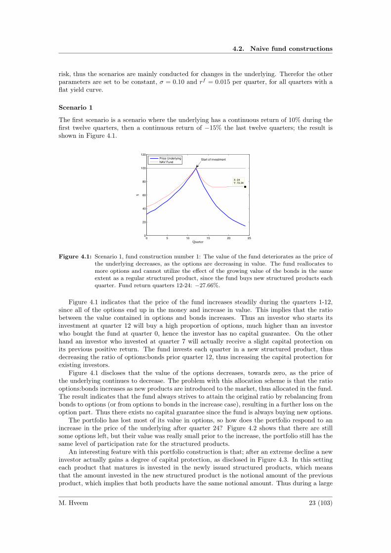
risk, thus the scenarios are mainly conducted for changes in the underlying. Therefor the otherparameters are set to be constant, σ = 0.10 and rf = 0.015 per quarter, for all quarters with aflat yield curve.
Scenario 1
The first scenario is a scenario where the underlying has a continuous return of 10% during thefirst twelve quarters, then a continuous return of −15% the last twelve quarters; the result isshown in Figure 4.1.
0 5 10 15 20 250
20
40
60
80
100
120
X: 24Y: 72.34
Quarter
$
Price Underlying
NAV FundStart of investment
Figure 4.1: Scenario 1, fund construction number 1: The value of the fund deteriorates as the price ofthe underlying decreases, as the options are decreasing in value. The fund reallocates tomore options and cannot utilize the effect of the growing value of the bonds in the sameextent as a regular structured product, since the fund buys new structured products eachquarter. Fund return quarters 12-24: −27.66%.
Figure 4.1 indicates that the price of the fund increases steadily during the quarters 1-12,since all of the options end up in the money and increase in value. This implies that the ratiobetween the value contained in options and bonds increases. Thus an investor who starts itsinvestment at quarter 12 will buy a high proportion of options, much higher than an investorwho bought the fund at quarter 0, hence the investor has no capital guarantee. On the otherhand an investor who invested at quarter 7 will actually receive a slight capital protection onits previous positive return. The fund invests each quarter in a new structured product, thusdecreasing the ratio of options:bonds prior quarter 12, thus increasing the capital protection forexisting investors.
Figure 4.1 discloses that the value of the options decreases, towards zero, as the price ofthe underlying continues to decrease. The problem with this allocation scheme is that the ratiooptions:bonds increases as new products are introduced to the market, thus allocated in the fund.The result indicates that the fund always strives to attain the original ratio by rebalancing frombonds to options (or from options to bonds in the increase case), resulting in a further loss on theoption part. Thus there exists no capital guarantee since the fund is always buying new options.
The portfolio has lost most of its value in options, so how does the portfolio respond to anincrease in the price of the underlying after quarter 24? Figure 4.2 shows that there are stillsome options left, but their value was really small prior to the increase, the portfolio still has thesame level of participation rate for the structured products.
An interesting feature with this portfolio construction is that; after an extreme decline a newinvestor actually gains a degree of capital protection, as disclosed in Figure 4.3. In this settingeach product that matures is invested in the newly issued structured products, which meansthat the amount invested in the new structured product is the notional amount of the previousproduct, which implies that both products have the same notional amount. Thus during a large
M. Hveem 23 (103)

Chapter 4. The Capital Protection Property
0 5 10 15 20 25 30 35 400
20
40
60
80
100
120
140
X: 36Y: 137.8
Quarter
$
Price Underlying
NAV Fund
Start of investment
0 5 10 15 20 250
20
40
60
80
100
120
X: 24Y: 108.1
Quarter
$
Price Underlying
NAV FundStart of investment
Figure 4.2: Extensions of scenario 1: The fund still has a lot of options held in the portfolio at quarter24, thus an appreciation in the underlying generates a high return even though the previousdecrease in the price.
0 10 20 30 40 50 600
20
40
60
80
100
120
Quarter
$
Price Underlying
NAV FundStart of investment
Figure 4.3: The fund has a floor which it does not cross (given a flat and constant yield curve) sincethe portfolio is in practice just rolling bonds.
decline the fund’s value has a period of 12 quarters, where the value repeats itself. This meansthat an investor at quarter 25 or 37 will in practice hold an identical position in bonds andoptions as seen in Figure 4.3 (note that this is a special case with the flat and constant yieldcurve), thus the portfolio is in some sense capital guaranteed over the twelve month period inthis case assuming a flat and constant yield curve, given the previous decline in the underlying.On the other hand this happens since the investor buys almost only bonds and a small fractionof options, thus the upwards potential is limited during the first quarters of a bull market.
Scenario 2
The second scenario is a scenario where the underlying has zero in return during the first twelvequarters, then a continuous return of −15% the last twelve quarters; the result is shown in Figure4.4. It can be expected that the outcome of this scenario should be very similar as the previousone, since the scenarios do not differ a lot from each other.
The fund value increases slightly during quarters 0-12 due to the interest of the bonds, whilethe option value declines due to the theta value of the options. As the underlying crashes duringquarters 12-24 so does the option value, thus most of the value is contributed by the bonds at
M. Hveem 24 (103)

4.2. Naive fund constructions
0 5 10 15 20 250
20
40
60
80
100
120
X: 24Y: 91.89
Quarter
$
Price Underlying
NAV FundStart of investment
Figure 4.4: Scenario 2, fund construction number 1: 0% in return of the underlying for twelve quarters,then continuous return of −15% each quarter. Fund return quarters 12-24: −8.11%.
quarter 15. This implies that, as the underlying continues to drop in price, there is not muchvalue left in options to affect, thus after a few quarters the fund is almost rolling bonds (sincethe decrease in option value each quarter reflects the increase of the bond value proportion ofthe total value).
Thus the portfolio actually has, in this scenario, a restricted downside over the time horizon.Hence the key to capital protection is to avoid holding products that are far in the money, sincethey have a large percentage of value contained in the options. Therefor the portfolio should berebalanced such that these assets are underweighted.
4.2.2 Naive fund construction number 2The naive fund construction number 2 differs slightly from the previous one. The first productfollows the same dynamics as in the previous subsection (100% capital guaranteed) but all theother products are not standardized. Instead the structured products issued after quarter 0 arecustomized in a way such that the ratio between the value contained in options and in bonds ismaintained relative stable for the fund. Thus every new structured product that is issued hasa participation rate such that the ratio between its option value and bond value, at issuance,equals the fund’s ratio between option value and bond value at this quarter. The price of thestructured product equals the price of the underlying at issuance, which is also the option’s strikeprice.
Every structured product matures three years after issuance, which means that the fund buysthe newly issued structured product every quarter with the payoff of the matured product (it isassumed that the fund can hold infinitesimal fractions of the structured products). Hence thefund will hold a maximum of twelve products each quarter.
The fund has to start somewhere and since the product prices are path dependent it isnecessary to start the fund three years prior that the investor invests in it (in this setting).Below follows a more detailed description of the fund (the same notations as in the previoussubsection will be used).
The bonds’ notional amounts depend on both the price of the underlying and the ratiooptions:bonds in the fund. The fund’s percentage of capital held in bonds at quarter i is givenas,
i−1∑j=0
βji(βji +Oji
)wji , and the percentage held in options as,i−1∑j=0
Oji(βji +Oji
)wji
M. Hveem 25 (103)

Chapter 4. The Capital Protection Property
thus the bond prices are given as,
βit =
Sie−rt(i+12−t), if i = 0
i−1∑j=0
βji(βji +Oji
)wjiSie12ri−rt(i+12−t), if i ≤ t ≤ i+ 12
0, otherwise
the participation rate of the option issued at quarter i is given as,
ki =
(Si − βii
)c (Si, Si, i, i+ 12, ri, σi)
=Si(1− e−12ri
)c (Si, Si, i, i+ 12, ri, σi)
, if i = 0
i−1∑j=0
Oji(βji +Oji
)wji Sic (Si, Si, i, i+ 12, ri, σi)
, otherwise
the value of the call option issued at quarter i at time t is given as,
Oit =
kiC (St, Si, t, i+ 12, rt, σt) , if i ≤ t ≤ i+ 11
kimax (St − Si, 0) , if t = i+ 12
0, otherwise
Hence the return between t− 1 and t for the structured product issued at quarter i is given as,
rit =βit +Oit
βit−1 +Oit−1− 1.
Now that it is known how the return for each structured product between each time period iscalculated the attention can again be turned towards the fund and how the portfolio weights arecalculated (since the return of the products each quarter depends on the weights the previousquarter). The portfolio weights will be given differently between quarters 0-11 and 12-24, sincethere is only one product available at quarter 0, only two products available at quarter 1 and soon. Thus the portfolio sells of some of its capital each quarter to allocate this in the newly issuedproduct, until there are twelve products. At quarter 0 the fund buys the newly issued product,at quarter 1 the fund sells of 50% of its possession to allocate in the newly issued product, atquarter 2 the fund sells of 33.33% of its possession to allocate in the newly issued product, atquarter 3 the fund sells of 25% of its possession to allocate in the newly issued product and so onuntil the first product matures, thus the portfolio weight for asset i at time t between quarters0-11 is given as,
wit | 0 ≤ t ≤ 11 =
(1 + rit
)wit−1
(1 + rt)T
wt−1
t
t+ 1, otherwise
wit = 1/(i+ 1), if i = t
wit = 0, if i > t
M. Hveem 26 (103)

4.2. Naive fund constructions
The first product matures during quarter twelve, thus there is a different allocation scheme toconsider from quarter twelve and onwards. The payoff of the matured product is as from quartertwelve reinvested in the newly issued product. Thus the portfolio weight for asset i at time tfrom quarter twelve and onwards is given as,
wit | t ≥ 12 =
(1 + rit
)wit−1
(1 + rt)T
wt−1, otherwise
(1 + ri−12t
)wi−12t−1
(1 + rt)T
wt−1, if i = t
0, if i ≤ t− 12 or i > t
The fund’s return is the weighted return of all the assets’ returns, thus the value of the fund isgiven as,
Vt =
{St, if t = 0
Vt−1 (1 + rt)T
wt−1, otherwise
Scenarios, underlying
The next step is to investigate some of the most important scenarios for the fund construction.These scenarios should stress the fund construction such that weaknesses are disclosed. Bydisclosing the worst-case scenarios it is possible to counter these characteristics by changing thefund construction.
Note that only some of the most unfavorable scenarios are disclosed in this thesis, less unfa-vorable scenarios are not disclosed, since they are not of importance.
As mentioned earlier, it is assumed that the investors have an investment horizon of threeyears and invest after three years (when the fund is announced on the market). It is importantthat the investment horizon coincides with the time to maturity of the structured products, sincethe individual structured product issued at the start of the investment provides absolute capitalguarantee for the investors and is their alternative investment. The scenarios are constructed tostress the negative outcomes and as shown in Section 4.2.4 the underlying is the most prevalentrisk, thus the scenarios are mainly conducted for changes in the underlying. Therefor the otherparameters are set to be constant, σ = 0.10 and rf = 0.015 per quarter, for all quarters with aflat yield curve.
Scenario 1
The first scenario is a scenario where the underlying has a continuous return of 10% during thefirst twelve quarters, then a continuous return of −15% the last twelve quarters; the result isshown in Figure 4.5.
Figure 4.5 shows that the value of the fund increases a lot as the underlying increases, due tothe increase of the options and their convexity. Thus an investor that buys the fund at quartertwelve buys a high proportion of options instead of bonds, since the fund maintains its ratio ofoptions:bonds relative stable when rebalancing. The fund’s proportion held in options convergestowards zero after seventeen quarters, thus bonds constitute almost all of the value. Figure 4.5discloses that the fund actually has a positive return after quarter 17, due to the positive returnof the bonds, even though the market continues to decrease, as the value of the option part isalready zero.
If the market goes down during twelve consecutive months an increase in the market wouldnot have any affect on the value of the fund, since it would not contain any options anymore.This fund construction creates a certain level of capital protection, but not in the desired way
M. Hveem 27 (103)

Chapter 4. The Capital Protection Property
0 5 10 15 20 250
20
40
60
80
100
120
X: 24Y: 61.68
Quarter
$
Price Underlying
NAV FundStart of investment
Figure 4.5: Scenario 1, fund construction number 2: Similar result as in the previous fund construc-tion. As the price of the underlying increases the ratio options:bonds increases heavilyto approximately 1:1 from 16.47:83.53, thus a new investor at quarter twelve can looseapproximately half of its investment. Fund return quarters 12-24: −38.32%.
since it is useless after a huge decline. It is also too risky since gains from the options are notreallocated to bonds, creating a huge downside after a bull market. Also, when the market turnsbust during consecutive quarters the portfolio reduces its participation heavily with the market,which can imply that the fund is only allocating in bonds and that it is no longer a structuredproducts fund.
Scenario 2
The second scenario is a scenario where the underlying has zero in return during the first twelvequarters, then a continuous return of −15% the last twelve quarters; the result is shown in Figure4.6.
0 5 10 15 20 250
20
40
60
80
100
120
X: 24Y: 116.4
Quarter
$
Price Underlying
NAV FundStart of investment
Figure 4.6: Scenario 2, fund construction number 2: The ratio options:bonds is very low since theprice of the underlying does not move until quarter 12. Thus the fall of the price of theunderlying does not really affect the value of the fund a lot. Fund return quarters 12-24:16.36%.
All options end out of the money, thus the option part’s value quickly converges towards zero
M. Hveem 28 (103)

4.2. Naive fund constructions
and the portfolio gains a positive return from the remaining bonds.
4.2.3 Analysis and summary
The most preferable fund construction is construction number one since it has less extremeoutcomes. Also fund construction number one will continue to participate in the market eventhough the market has decreased a lot. The fund also provides capital protection, when themarket has gone up, for investors who experienced the bull-market.
Based on these results it is easy to conclude that there is a big advantage to rebalance theportfolio at intermediate time points so that the ratio options:bonds does not exceed a certainlimit. This implies that it is possible to protect new investors from for example scenario 1. It isalso desirable to increase the ratio options:bonds in the same way as it is done in fund constructionnumber 1 after a market crash, if the fund wants to increase the possibility of appreciation, butthis should not be conducted when trying to minimize the risk. Using the allocation scheme infund construction number 1 implies that the fund slowly rebalances towards its original ratiooptions:bonds. On the other hand rebalancing up the ratio options:bonds each quarter when ithas decreased under a certain limit would imply that the portfolio’s risk increases i.e. there arepros and cons with every decision.
Fund construction number 2 is not desirable at all since it is a very risky investment strategyand does not hold the desired characteristics.
Concluded, it is important that the allocation scheme has a focus on rebalancing the rateoptions:bonds, where there exists a maximum acceptable limit. This can be done by for examplesolving a linear optimization problem.
The question now arises regarding how the option portfolio should be constructed, i.e. howthe weights in the different options (and thus also the structured products) should be constructedto retain as much capital protection as possible. The next section investigates how an investorshould allocate the option portfolio to have as little downside risk as possible. The reason whyit is possible to generalize the result of options to the structured products is that a change inthe underlying is the most prevalent risk of the structured products, which will be discussed inthe next subsection.
4.2.4 Prevalent risk factors
This short subsection discusses the most prevalent risk factors for an ELN. It is important todetermine the most prevalent risk factors to be able to construct a portfolio of structured productssuch that the risk is minimized.
The most volatile part of a structured product is the option, the bond is less sensitive tomovements affecting its price, i.e. the yield curve. Consider an Equity-Linked-Note with a priceof $100, price of the underlying of $100, ytm = 0.06, σ = 0.2 p.a. and a time to maturity of threeyears. The ratio options:bonds would be 16.47:83.53, a shift of the underlying downwards of 50%would induce a decrease of the product’s value of 15.9743. The yield to maturity would haveto increase to 13.08% to cause a price drop that big. There is not a huge risk with changes inthe yield curve that are not extreme since if the yield curve goes up bonds will be less expensiveand the bonds bought will generate a higher return, as seen in Figure 4.7 which depicts a hugechange in the interest rate. Also the interest rate risk is very small for buy and hold strategies,since the investor is guaranteed a fixed amount in the future, thus a fixed yield.
Figure 4.8 depicts the sensitivity of an ELN w.r.t. the underlying and the interest rate, theELN is much more sensitive to changes in the underlying than in the yield curve. Thus it ismore important to focus on changes in the underlying than the interest rate. When consideringa buy and hold portfolio (which most funds practice, it is reasonable to assume that the wholeportfolio will not rebalanced each quarter due to transaction costs) it is a much larger risk thatthe option is out of the money close to maturity than that the bond has a low price close to
M. Hveem 29 (103)

Chapter 4. The Capital Protection Property
0 5 10 15 20 250
20
40
60
80
100
120
X: 24
Y: 100.3
Quarter
[%]
Interest Rate
NAV FundStart of investment
Figure 4.7: The interest rate goes from 2% p.a. to 14% p.a. during just a few quarters. The investordoes not have a negative return over the whole period. The big risk is if a change occursjust prior to the end of the investment horizon, but as it can be seen, the impact is stilllimited.
maturity. Thus the interest rate risk of holding an existing bond is much smaller than holdingthe option.
0
50
100
150
200
0
5
10
15
60
80
100
120
140
160
St
T = 3
Interest Rate r [%]
EL
N P
rice [
%]
70
80
90
100
110
120
130
140
150
0
50
100
150
200
0
5
10
15
90
100
110
120
130
St
T = 0.5
Interest Rate r [%]
EL
N P
rice [
%]
95
100
105
110
115
120
125
Figure 4.8: The surface plots describe how changes in the yield and price of the underlying affect theprice of an ELN. σ = 0.2, K = 100, as time decreases so does the sensitivity to changes inthe yield curve.
There may also be a risk with a decrease in volatility. But, as a consequence of the definitionof volatility, the volatility increases as the price goes down (since the drift is in general positive),thus the two risk factors counter each other’s impact on the price. Thus a decrease in volatilityis not a big concern since it happens when the price of the underlying goes up, which affects theoption price more than the volatility as seen in Figure 4.9.
Hence it is possible to generalize the optimal allocation of options, in min risk sense, to aportfolio of structured products since the options in the ELNs are significantly more risky thanthe bonds. The next section will therefor investigate how the option portfolio should be allocatedto minimize the negative outcomes.
M. Hveem 30 (103)

4.3. Investigation of the option portfolio
0
50
100
150
200
0
10
20
30
40
50
0
20
40
60
80
100
St [%]Volatility σ [%]
Op
tio
n P
rice
0
10
20
30
40
50
60
70
80
90
Figure 4.9: The surface plot describes the relationship between changes in volatility and the price,price is the dominant factor. Strike K = 100, r = 0.06, T = 3.
4.3 Investigation of the option portfolio
The purpose of this section is to investigate how the option portfolio should be allocated to min-imize the negative outcomes in sense of the underlying, since the minimum-risk option portfolioshould in most cases yield the minimum-risk ELN portfolio.
The options are priced with Black-Scholes formula as given in Equation 3.1. The optionprices are assumed to not be smaller than 0.5% of the price of the underlying, before maturity,to prevent unrealistic results. Without setting such boundaries some options may have returnsin the size of 1030 between two quarters.
The study covers different portfolio constructions (only those relevant are shown) and howthe scenarios are modeled to stress the different portfolio allocations. The section also generatesa recommendation regarding how an option portfolio should be allocated such that the risk isminimized.
4.3.1 Portfolio construction and modeling
The portfolios that are investigated consist of only plain vanilla at-the-money call options atissuance on the underlying index. To test which portfolio setups that are best in min risk sensethe study will conduct Monte Carlo simulation. It is not important to replicate a certain index,since the study is looking for patterns, which should be independent as much as possible of theassumptions of the underlying. The index OMXS30 at Nasdaq OMX serves as a base for thesimulation, thus daily log returns are gathered between 1st of October 2009 to 30th of September2010. The log returns are fitted to a student’s t-distribution to attain slightly heavier tails thanfor the normal distribution, as well as a better fit. Since the investigation is investigating patternsand worst-case outcomes it does not really matter what the drift µ is set to be, thus µ is forsimplicity set to zero, the other fitted parameters for the t-distribution are: σ = 0.0105, ν = 5.69(on a days basis, it is not important what the actual parameters are since the focus lies onpatterns, which should not be sensitive to the distribution of the underlying).
The following parameters are also used: rf = 6% p.a. and the volatility used when pricingthe options is the actual realized volatility during the period of 20.5% p.a.
M. Hveem 31 (103)
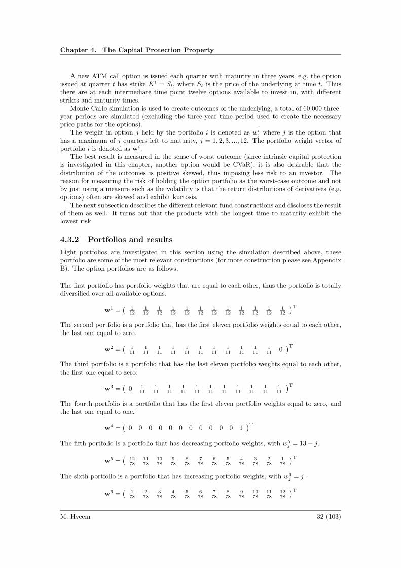
Chapter 4. The Capital Protection Property
A new ATM call option is issued each quarter with maturity in three years, e.g. the optionissued at quarter t has strike Kt = St, where St is the price of the underlying at time t. Thusthere are at each intermediate time point twelve options available to invest in, with differentstrikes and maturity times.
Monte Carlo simulation is used to create outcomes of the underlying, a total of 60,000 three-year periods are simulated (excluding the three-year time period used to create the necessaryprice paths for the options).
The weight in option j held by the portfolio i is denoted as wij where j is the option thathas a maximum of j quarters left to maturity, j = 1, 2, 3, ..., 12. The portfolio weight vector ofportfolio i is denoted as wi.
The best result is measured in the sense of worst outcome (since intrinsic capital protectionis investigated in this chapter, another option would be CVaR), it is also desirable that thedistribution of the outcomes is positive skewed, thus imposing less risk to an investor. Thereason for measuring the risk of holding the option portfolio as the worst-case outcome and notby just using a measure such as the volatility is that the return distributions of derivatives (e.g.options) often are skewed and exhibit kurtosis.
The next subsection describes the different relevant fund constructions and discloses the resultof them as well. It turns out that the products with the longest time to maturity exhibit thelowest risk.
4.3.2 Portfolios and resultsEight portfolios are investigated in this section using the simulation described above, theseportfolio are some of the most relevant constructions (for more construction please see AppendixB). The option portfolios are as follows,
The first portfolio has portfolio weights that are equal to each other, thus the portfolio is totallydiversified over all available options.
w1 =(
112
112
112
112
112
112
112
112
112
112
112
112
)TThe second portfolio is a portfolio that has the first eleven portfolio weights equal to each other,the last one equal to zero.
w2 =(
111
111
111
111
111
111
111
111
111
111
111 0
)TThe third portfolio is a portfolio that has the last eleven portfolio weights equal to each other,the first one equal to zero.
w3 =(
0 111
111
111
111
111
111
111
111
111
111
111
)TThe fourth portfolio is a portfolio that has the first eleven portfolio weights equal to zero, andthe last one equal to one.
w4 =(
0 0 0 0 0 0 0 0 0 0 0 1)T
The fifth portfolio is a portfolio that has decreasing portfolio weights, with w5j = 13− j.
w5 =(
1278
1178
1078
978
878
778
678
578
478
378
278
178
)TThe sixth portfolio is a portfolio that has increasing portfolio weights, with w6
j = j.
w6 =(
178
278
378
478
578
678
778
878
978
1078
1178
1278
)TM. Hveem 32 (103)

4.3. Investigation of the option portfolio
The seventh portfolio is a portfolio that has equal portfolio weights in assets 2-10, zero otherwise.
w7 =(
0 19
19
19
19
19
19
19
19
19 0 0
)TThe eighth portfolio is a portfolio that has equal portfolio weights in assets 2-11, zero otherwise.
w8 =(
0 110
110
110
110
110
110
110
110
110
110 0
)TThe results for the different option portfolios are disclosed in Figure 4.10, there are also
additional option portfolios disclosed in Appendix B.Figure 4.10 and Appendix B show that the portfolios where the options closest to maturity
are underweighted have “better” distributions since they exhibit less negative skewness. Also theworst-case outcome is much better for portfolios that have underweighted the options closest tomaturity. Fewer number of assets in the portfolio results in, in most cases, a more risky portfolio,both in worst-case and in distribution. Notable is that the portfolio that has the best worst-caseoutcome is the portfolio that holds 100% of its holdings in the option with the longest time tomaturity (Portfolio 4).
Figure 4.12a shows that options with a longer time to maturity are less sensitive to thechanges in time (θ = ∂P
∂t ). Thus the value reduction coming in form of the reduction in time,ceteris paribus, is less if the investor holds options with a long time to maturity. Also the delta(∆ = ∂P
∂s ) for options that are in the money is higher for options close to maturity than optionswith a long time to maturity as depicted in Figure 4.12b.
As a fund manager it would be quite unreasonable to allocate all the capital in the sameasset, thus it is adequate to demand that the fund diversifies itself, to not overweight. Usuallya portfolio manager is not allowed to invest more than a certain percentage (say 30%) in aparticular asset, it is in this case beneficial to diversify along almost all options, except the oneclosest to maturity (which has the highest risk, since it might be “all or nothing”). The resultsin Figure 4.10, B.1 and B.2 indicate that it does not really matter how the portfolio diversifiesamongst the assets since the results are quite similar as long as the portfolio holds a relativelarge proportion of the holdings in products with a longer time to maturity. Thus it might bereasonable to diversify by holding only four options with a long time to maturity as in Portfolio16 in Appendix B or for example diversify over the whole spectrum and attain approximatelythe same results.
It would be desirable if the return distribution for the portfolio of options over 36 monthswould look somewhat similar to the return distribution of a single option from issue to maturityas seen in Figure 4.11. The results shown in the figures indicate that it is not possible to attainthe same type of distribution as for a single option when investing in several options over 36months.
−5 0 5 10 15 200
1000
2000
3000
4000
5000
6000
7000
Plain vanilla option return
Return [%]
Outc
om
es
Figure 4.11: The histogram shows the distribution of a plain vanilla option’s one-year return, issuedATM (T = 1).
M. Hveem 33 (103)

Chapter 4. The Capital Protection Property
−0.25 −0.2 −0.15 −0.1 −0.05 0 0.05 0.1 0.150
20
40
60
80
100
120
140
160
180
Option portfolio average monthly returns (36 months periods)
Average return per month
Outc
om
es
(a) Portfolio 1, −22.37%.
−0.25 −0.2 −0.15 −0.1 −0.05 0 0.05 0.1 0.150
20
40
60
80
100
120
140
160
Option portfolio average monthly returns (36 months periods)
Average return per month
Outc
om
es
(b) Portfolio 2, −21.88%.
−0.2 −0.15 −0.1 −0.05 0 0.05 0.1 0.150
20
40
60
80
100
120
140
160
180
Option portfolio average monthly returns (36 months periods)
Average return per month
Ou
tco
mes
(c) Portfolio 3, −17.64%.
−0.2 −0.15 −0.1 −0.05 0 0.05 0.1 0.150
50
100
150
200
250
Option portfolio average monthly returns (36 months periods)
Average return per month
Outc
om
es
(d) Portfolio 4, −16.15%.
−0.3 −0.25 −0.2 −0.15 −0.1 −0.05 0 0.05 0.1 0.150
20
40
60
80
100
120
140
160
180
Option portfolio average monthly returns (36 months periods)
Average return per month
Outc
om
es
(e) Portfolio 5, −27.69%.
−0.25 −0.2 −0.15 −0.1 −0.05 0 0.05 0.1 0.150
20
40
60
80
100
120
140
160
180
200
Option portfolio average monthly returns (36 months periods)
Average return per month
Outc
om
es
(f) Portfolio 6, −20.71%.
−0.2 −0.15 −0.1 −0.05 0 0.05 0.1 0.150
20
40
60
80
100
120
140
160
180
Option portfolio average monthly returns (36 months periods)
Average return per month
Outc
om
es
(g) Portfolio 7, −19.80%.
−0.2 −0.15 −0.1 −0.05 0 0.05 0.1 0.150
20
40
60
80
100
120
140
160
180
Option portfolio average monthly returns (36 months periods)
Average return per month
Outc
om
es
(h) Portfolio 8, −18.91%.
Figure 4.10: Histograms over the outcomes for option portfolios 1-8, the worst-case average 36 monthreturn is given in the caption.
M. Hveem 34 (103)

4.3. Investigation of the option portfolio
An optimal portfolio would be positive skewed, with a limited downside. The most benefi-cial construction fulfilling these criteria is Portfolio 3, as indicated in Figure 4.10c (as well asconsidering the worst-case outcome). Hence it is important to diversify over a large set of assetsto reduce the risk, when constructing a portfolio only consisting of options. On the other handas the time to maturity decreases, the risk increases (the theta and delta (given that the optionis in the money) in particular, as disclosed in Figure 4.12). Thus when constructing a portfoliowith structured products it is important to not overweight in the shorter tenors.
The main result is that the fund should diversify over a number of assets and also avoidinvesting in the products with a short time to maturity. Next follows an analysis of how theresults found in Section 4.2 and in this section should be combined to construct a desirablestructured products fund.
050
100150
200
0
10
20
30
40
−4.5
−4
−3.5
−3
−2.5
−2
−1.5
−1
−0.5
0
St
Months to maturity
Op
tio
n T
het
a (Θ
)
(a) The plot describes a plain vanilla call option’s theta(time value), the theta is heavily decreasing in time,implying that the holder looses a lot of capital froma time change close to maturity, ceteris paribus.
0
50
100
150
2000
10
20
30
40
0
0.2
0.4
0.6
0.8
1
Months to maturityS
t
Op
tio
n D
elta
(∆
)
(b) The plot describes a plain vanilla call option’s delta,options closer to maturity are more sensitive whenthey are in the money than options with a longertime to maturity.
Figure 4.12: The Figure a) illustrates an option’s theta value, the Figure b) illustrates an option’sdelta value for different levels of in the money and time to maturity.
4.3.3 Analysis and implications
In this subsection follows a combination of a summary, an analysis and a description of theimplications from the studies in this chapter so far.
It is known from Section 4.2 that it is desirable to rebalance the portfolio when the ratiooptions:bonds exceeds a predetermined level (which depends on the risk profile of the fund) tolimit the downside risk. The reason why the ratio options:bonds suddenly exceeds a certain levelis (most often) due to either an increase in the price of the underlying (increasing the valueof the options) or in the yield curve (reducing the value of the bonds). Thus by rebalancingthe portfolio the downside risk is limited since the proportion of options is reduced. This isan important concept since it protects new investors, the fund must be able to guarantee newinvestors that they do not buy more than a certain percentage of options. Without this guaranteethe purpose of the fund is lost, by appealing to investors’ loss aversion (Shefrin, 2002, [35]).
By rebalancing the portfolio after a period of growth the value held in bonds increases. Thusthe existing investors will receive a certain level of capital protection on their gains. The tradeoffis that the portfolio at the same time limits the upside of the investment (the tradeoff between riskand return). These characteristics appeal to psychological concepts within Behavioral Finance,where investors tend to sell assets too early during growth, since they are conservative andpeople do not expect the market to continue appreciating (disposition effect) (Frazzini, 2006,[15]; Kahneman and Tversky, 1979, [26]). Thus investors want to rebalance their portfolio after
M. Hveem 35 (103)

Chapter 4. The Capital Protection Property
a period of appreciation.During bear markets, when the portfolio decreases in value, it may be desirable to rebalance
the portfolio’s ratio of options:bonds towards a desired level. The rebalancing should not beconducted in the same manner as when the ratio exceeds a certain level, instead it may bedesirable to slowly re-establish the portfolio’s ratio options:bonds to the original level. Withoutthis reallocation the fund will not have as much upside for new investors. Thus it is a balanceact for the fund how it should change the ratio options:bonds in a way that both new investorsand current investors appreciate. The next section will investigate how this ratio/level shouldbe chosen and its implications on downside risk.
Since Equity-Linked Notes are considered in this paper the options are far more risky than thebonds, thus by allocating the portfolio according to the minimum risk choice w.r.t. the optionsshould also yield the minimum risk choice for the structured products.
As stated previously, there is no need to investigate changes of volatility, since the volatilityand the price of the underlying usually counter each other (Glot, 2005, [16]). Thus the impactof volatility can be neglected when choosing portfolio weights. The inflation goes up whenthe market goes up, thus also interest rates. When markets go down, investors flee to saferinstruments such as bonds, thus pushing up the price and decreasing the yield. This implies thatthe price changes of bonds and call options are negatively correlated.
As seen in Section 4.3 the best choice to minimize the downside risk for a portfolio of optionsis by diversification in the longer (and middle) tenors. Thus it is not desirable to hold positionsin options that have a short time to maturity.
When considering a portfolio of structured products it might be non-desirable to overweightthe newly issued products during bear markets since they will have a substantial proportion ofoption value in them compared to the other products. Thus if the portfolio overweights/allocatesto the newly issued ELNs it will always reallocate capital to newly issued options, which is notdesirable in bear markets. Hence instead of allocating according to Portfolio 3, as when onlyconsidering an option portfolio, a higher degree of capital protection during bear markets will beattained by investing using either Portfolio 7 or 8. Thus it is reasonable to invest using Portfolio3 in general and after drops in the index allocate the portfolio according to Portfolio 7.
It is desirable to rebalance the portfolio such that the ratio options:bonds are held undercontrol, but how should this be conducted, for which levels etc? These issues will be investigatedin the next section where a comparison with existing mixed funds results in optimal choices ofthe ratio options:bonds.
4.4 Comparison with competition
A lot of assumptions have to be made in able to construct the fund. One way to make adequateassumptions is to relate to the fund’s competition. Investors will not invest in the fund if it is notcapable of beating its competition, at least at some aspects. The comparison will be based onthe results found in the previous sections. Thus the purpose of this section is to investigate howa potential structured products fund (SPF) performs in relation to its competition (mixed funds)during extreme scenarios. The analysis results in appropriate boundaries for the percentage ofvalue in the SPF contributed by options given a certain competing/benchmark fund.
A competing fund is a fund that has the same client base as the SPF. Thus it is imperativeto establish the SPF’s client base, so that a competing benchmark fund can be identified. Afterthat the competing fund has been identified the study investigates how different SPFs can beconstructed, such that the SPF provides a higher degree of capital protection than the benchmarkfund.
The different constructions are both stress tested with predefined extreme scenarios as wellas simulated scenarios. The different SPF strategies are also backtested against historical data.
The section covers two types of SPFs, one where the weights are based on the possession inthe structured products and one SPF where the weights in the structured products are based on
M. Hveem 36 (103)

4.4. Comparison with competition
the possession in the options. It turns out that the second one is more theoretical than the firstone. The result in this section indicates that a structured products fund should try to have apossession of 5-25% option value attained in the portfolio, with a target level of 15% to be moreattractive for investors in min risk sense than a competing mixed fund.
4.4.1 Client baseThe fund based on structured products has a high focus on capital protection. Thus the investorsthat it is suitable for are those who are looking for investments with a limited downside, ora small risk, as well as a possibility to have a return connected to the market. These arerisk-aversive investors who usually are looking for a combination of bonds and stocks. Todaymany of these investors invest in mixed funds, which diversify their portfolios in both debtand equity instruments to lower the risk level, hence it is this alternative which is an adequatebenchmark. Thus mixed funds are identified to be the competition to the SPF, hence thestructured products fund must provide a lower downside risk than competing mixed funds to bean attractive investment alternative.
Next follows a more detailed description of the benchmark fund.
4.4.2 Benchmark fund
It is assumed that a reasonable benchmark fund is a mixed fund that aims at holding 30% (εbench)of its capital in stocks and 70% in bonds with up to three years until maturity (to match theSPF). The benchmark fund rebalances its position every three months, if the level of stocks heldis not within 30% ± 10% (δbench). The investment within stocks is considered in this study tobe conducted in the index (or an ETF), which is also the underlying for the SPF. An exampleof a price development of this type of benchmark fund is disclosed in Figure 4.13. The figureshows that the benchmark fund gains value as the market is appreciating and does not decreasesignificantly as the market takes a turn for the worse. Thus it has some of the desired propertiesfor a SPF, imposing an adequate benchmark. The focus is now turned to the construction of thestructured products fund.
0 50 100 15050
100
150
200
250
300
350
400
450
Month
$
Price Underlying
NAV Benchmark
Figure 4.13: The co-movements of the underlying and the benchmark fund, for εbench = 0.3, δbench =0.1 and r = 0.06 p.a, random scenario.
4.4.3 Structured products fund 1The fund constructions in this section are based on the results gained in Section 4.2 and 4.3, thusthe portfolio diversifies broadly amongst the available products. Portfolio 7 will be used, since
M. Hveem 37 (103)

Chapter 4. The Capital Protection Property
the test is conducted for bear markets (in Appendix C results for Portfolio 3 are disclosed), thusthe portfolio holds equal weights in products i = 2 − 10 where i denotes the maximum numberof quarters until maturity for the product as previously.
A new capital guaranteed structured product is issued each quarter with maturity in threeyears, price equal to the price of the underlying and also the notional amount of the bond, asin Section 4.2.1. The fund also has the possibility of investing in short-term debt, in this casebonds that have maturity the next quarter. Thus the fund can by investing in the short-termdebt reduce the percentage of value placed in options. A target level of options held in the fund’sportfolio is also introduced, this target level is the desired percentage of the fund’s value thatshould be constituted by options, let denote this target level as εSPF. Notable is that the fundis not allowed to short the short-term debt.
The fund rebalances its portfolio of structured products each quarter as previously, accordingto the weights and maturity amongst the structured products, and also the proportion placed inadditional bonds.
The fund adjusts the proportion placed in the short-term debt subject to its level of optionvalue as a percentage of the total fund. The portfolio is allowed to deviate a percentage δSPF fromits target level of options. Thus the portfolio is rebalanced if the percentage of value contributedby the options exceeds εSPF + δSPF (or is less than εSPF− δSPF) by allocating in short-term debtrather than the structured products, thus attaining the target level.
w̃ denotes the weight vector for the structured products excluding the short-term debt (theweights amongst the structured products), the weight in the short-term debt at time t is denotedas wbt . Thus the actual weights (except wbt ) for each time-period is given by:
wt =(1− wbt
)w̃,
and since the focus lies on Portfolio 7 from Section 4.3 the following weights are used,
w̃ =(
0 19
19
19
19
19
19
19
19
19 0 0
)T.
Note that wb0 = 0 and w0 = w̃, the proportion of value of the fund contributed by bonds isdenoted αb, and αo is the proportion of value of the fund contributed by options. Which givesus the following definitions,
αbt = wbt +(1− wbt
) n∑i=1
w̃iβit
βit +Oit,
αot =(1− wbt
) n∑i=1
w̃iOit
βit +Oit,
where n is the number of available products (12 in this case), thus the portfolio is rebalancedeach quarter if,
αot ≤ εSPF − δSPF or αot ≥ εSPF + δSPF.
The portfolio is rebalanced with the aim that αo should equal εSPF, this is not always possiblesince it is not allowed to short the short-term debt, which implies that the new portfolio weightsare given as,
wnewt =
wtεSPF
αot, if
∑i
witεSPF
αot≤ 1
w̃, if∑i
witεSPF
αot> 1
M. Hveem 38 (103)

4.4. Comparison with competition
these weights are the weights excluding the short-term debt, thus the new allocation in theshort-term debt is as follows,
wbt = 1− 1Twnewt .
The fund is not allowed to short the short-term debt (to minimize the risk), thus it cannot holdnegative positions in wbt . This implies that the short-term debt is used as a safe haven to avoida too high exposure to the market.
The purpose with the following subsections is to determine the adequate levels for εSPF andδSPF such that the fund has a greater protection (towards extreme downside risk) than thebenchmark portfolio(s), and still has a good upside potential. The levels will be determined suchthat the SPF provides a greater capital protection for market crashes of −20% p.a. and more.
4.4.4 Scenarios
This subsection describes the scenarios that the SPF and benchmark fund are stressed with. Thescenarios are not simulated since it is desirable that the SPF provides capital protection for somespecified market crashes.
The scenarios should stress the SPF and the benchmark fund towards negative outcomes, thusexpose the funds in an extent where they disclose weakness (which is a market crash immediatelyafter a strong increase in the market, as seen in the previous sections). The focus lies on scenarioswith an up-going market followed by a market crash (as the worst-case scenarios in Section 4.2),five different scales of market crashes are investigated, −80%,−50%,−30%,−20% and −10%p.a. during four years. Two different settings prior to the crash will be investigated, the firstsetting with a bull market with a return of 30% in return p.a. between months 0-48 (Scenario A).The second scenario is quite similar, 30% return p.a. during months 0-48 and a return of 50%each month for months 48-50 (Scenario B). The idea is that since the funds can only rebalanceto short-term debt every three months that the funds can be stressed even more if an extremeincrease occurs during a period where the funds cannot rebalance. Thus these two types ofscenarios should cover the worst types of extreme outcomes for the funds (for more extremescenarios please consult Appendix C).
Hence the market crash in Scenario A is between months 48-96 and in Scenario B betweenmonths 50-98.
After the crash the market experiences an increase of 30% p.a. until month 144 (12 years).An annual interest rate of 6% is assumed for the bonds as well as the short-term debt (flat yieldcurve is assumed for simplicity), the scenarios can be seen in Figure 4.14.
The reason why predefined stressed scenarios are studied instead of simulation in this sub-section is that the study is trying to stress test the funds in particular scenarios and see if theSPF has the desired properties. Also it is imperative that the results gained from this study areindependent of the models selected for the underlying and that they can be generalized to anydistribution or market model, thus it is appropriate to select scenarios without simulation.
The next subsection covers the results over how the funds perform in the different scenariosand how the results should be interpreted.
4.4.5 Results, structured products fund vs benchmark
The focus lies on the worst-case outcomes of the SPF (based on Portfolio 7) and the benchmarkfund given different scenarios and values for ε and δ. The objective is to construct a SPF suchthat it has more favorable worst-case outcomes than the benchmark portfolio.
Various results are disclosed in Figure 4.14, Table 4.1 and 4.2. Table 4.1 discloses the resultregarding the SPF, its worst-case outcome given the different scenarios, εSPF and δSPF. Table 4.2discloses in the same manner the result regarding the benchmark fund, its worst-case outcomegiven the different scenarios, εbench and δbench.
M. Hveem 39 (103)

Chapter 4. The Capital Protection Property
Return IndexMonths 48-96 /50-98 p.a.
εSPF δSPF Scenario A Worst-Case Return
Scenario B Worst-Case Return
-80% 1 1 -18.53% -56.07%-80% 0.3 0.1 -18.53% -37.62%-80% 0.25 0.1 -11.95% -32.18%-80% 0.20 0.1 -11.35% -22.62%-80% 0.15 0.1 -2.85% -15.20%-80% 0.15 0.05 -2.54% -19.22%-80% 0.10 0.05 -1.06% -9.59%-50% 1 1 -17.46% -48.50%-50% 0.3 0.1 -17.46% -33.04%-50% 0.25 0.1 -11.57% -25.42%-50% 0.20 0.1 -11.03% -18.39%-50% 0.15 0.1 -3.42% -11.48%-50% 0.15 0.05 -6.20% -16.71%-50% 0.10 0.05 -1.82% -7.59%-30% 1 1 -16.64% -37.40%-30% 0.3 0.1 -16.64% -22.49%-30% 0.25 0.1 -13.24% -19.26%-30% 0.20 0.1 -11.31% -13.63%-30% 0.15 0.1 -5.00% -5.41%-30% 0.15 0.05 -7.32% -10.23%-30% 0.10 0.05 -3.45% -3.54%-20% 1 1 -14.60% -26.84%-20% 0.3 0.1 -14.60% 14.64%-20% 0.25 0.1 -11.13% -10.59%-20% 0.20 0.1 -9.72% -6.15%-20% 0.15 0.1 -3.95% 0.34%-20% 0.15 0.05 -6.09% -3.38%-20% 0.10 0.05 -2.55% 2.90%-10% 1 1 -9.60% -14.08%-10% 0.3 0.1 -9.60% -4.75%-10% 0.25 0.1 -6.78% -1.81%-10% 0.20 0.1 -5.81% 0.43%-10% 0.15 0.1 -1.65% 3.82%-10% 0.15 0.05 -3.11% 1.23%-10% 0.10 0.05 0.22% 4.79%
Table 4.1: SPF 1: Worst-case outcomes for SPF 1 based on Portfolio 7 given scenarios A and B, εSPF
and δSPF, the worst-case period is always the 36 month following the initiation of the crash.
M. Hveem 40 (103)
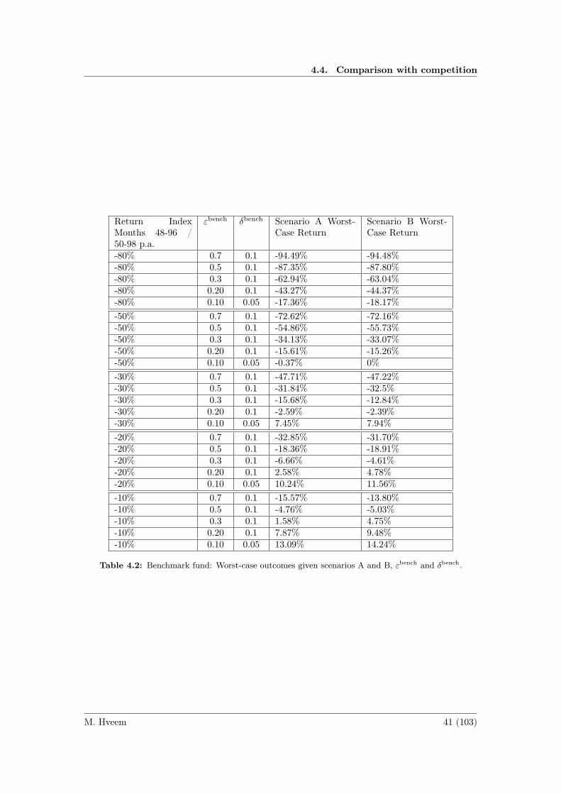
4.4. Comparison with competition
Return IndexMonths 48-96 /50-98 p.a.
εbench δbench Scenario A Worst-Case Return
Scenario B Worst-Case Return
-80% 0.7 0.1 -94.49% -94.48%-80% 0.5 0.1 -87.35% -87.80%-80% 0.3 0.1 -62.94% -63.04%-80% 0.20 0.1 -43.27% -44.37%-80% 0.10 0.05 -17.36% -18.17%-50% 0.7 0.1 -72.62% -72.16%-50% 0.5 0.1 -54.86% -55.73%-50% 0.3 0.1 -34.13% -33.07%-50% 0.20 0.1 -15.61% -15.26%-50% 0.10 0.05 -0.37% 0%-30% 0.7 0.1 -47.71% -47.22%-30% 0.5 0.1 -31.84% -32.5%-30% 0.3 0.1 -15.68% -12.84%-30% 0.20 0.1 -2.59% -2.39%-30% 0.10 0.05 7.45% 7.94%-20% 0.7 0.1 -32.85% -31.70%-20% 0.5 0.1 -18.36% -18.91%-20% 0.3 0.1 -6.66% -4.61%-20% 0.20 0.1 2.58% 4.78%-20% 0.10 0.05 10.24% 11.56%-10% 0.7 0.1 -15.57% -13.80%-10% 0.5 0.1 -4.76% -5.03%-10% 0.3 0.1 1.58% 4.75%-10% 0.20 0.1 7.87% 9.48%-10% 0.10 0.05 13.09% 14.24%
Table 4.2: Benchmark fund: Worst-case outcomes given scenarios A and B, εbench and δbench.
M. Hveem 41 (103)

Chapter 4. The Capital Protection Property
The structured products fund provides, as the tables indicate, (in general for the same levelsof ε and δ as the benchmark fund) a much higher safety in extreme downturn markets (−80%drop), since it does not short bonds to reallocate its portfolio. It is not a huge difference betweenthe worst-case outcomes for different extreme scenarios (−30 to −80% drops) when regardingthe SPF (Table 4.1), since the value of the options does not decrease a lot more in the −80%case than in the −30% case. Table 4.2 shows that the benchmark fund on the other hand suffersto a high extent when the index has huge negative returns since it reallocates every three-monthto the index, thus not providing a limit where it cannot lose more capital. It is important tonotice that the SPF appreciates quite a lot when the market starts to go up again, which isvery desirable as seen in Figure 4.14. The SPF has a greater upside for huge increases thanthe benchmark fund (Figure 4.14). Notable is that it takes longer time for the SPF than thebenchmark fund to appreciate after the market turns bust, it is this effect which also creates thecapital protection property, since it takes a few quarters to increase the participation rate.
Table 4.1 shows that the SPF is in general more sensitive to a large drop in the stock marketafter an extreme increase without having the possibility to rebalance the portfolio (Scenario B)than to Scenario A. The SPF is less sensitive to Scenario B if it is only followed by a correctionin the market (return of −10% to −20% p.a.). This is due to that the SPF does not suffer a lotof the decline between months 50-51 and the portfolio is rebalanced at month 51 to lower levels,thus making it less sensitive to a market crash. On the other hand the portfolio does not benefitso much of the rebalancing possibility during month 51 in the case of a huge decline betweenmonths 50-51, such as in the −80% drop scenario (Table 4.1). Notable is that the results arequite similar if there is a drop of −80% per month between months 50-51, the results for thisscenario are disclosed in Appendix C1.
Since the fund rebalances its portfolio at month 48 a sense of upper loss limit, which theinvestor cannot lose more than if it starts its investment horizon at quarter 48, is created. Thisimplies that if the fund experiences a total market crash (−100%) the investor still holds itsposition in bonds, while the market linked assets would by worth zero. Thus the investor losesa “maximum” (in sense of the underlying) of ε + δ which is applicable to both the SPF andbenchmark fund. But the value invested in options is convex and more volatile than investingin the underlying. Thus a decline with 50% may erase almost all value attained in the options.Hence the criteria εSPF + δSPF < εbench + δbench must hold if the SPF should have a highercapital protection for declines of the scale 30-50%.
One interesting property that is not disclosed in the tables is that the fund can limit itsdownside significantly using two different δSPF, one for the upside (δSPF
+ ) and one for the downside(δSPF− ). By increasing the downside limit δSPF
− the fund has a higher tolerance for holding short-term debt than when having a symmetrical δSPF. Important to notice is that as δSPF
− increasesit will be harder for the SPF to appreciate after a bear market since it accepts higher levels ofshort-term debt and does not reallocate in a high extent to structured products.
Next follows an analysis regarding the results and an interpretation regarding their implica-tions for a portfolio manager.
4.4.6 Analysis and summary
As mentioned earlier an adequate benchmark fund is a fund which has εbench = 0.3 and δbench =0.1. Thus the desired weights of εSPF and δSPF should provide better capital protection againstdownside risk than the benchmark fund. It is reasonable to demand that the SPF should be lesssensitive to market drops of −20% p.a. or more (it is difficult to find portfolio weights for thefund that would be less sensitive at a −10% market drop2, as seen in Table 4.1 and 4.2). Byinspecting Table 4.1 and 4.2 it is easy to notice that the adequate levels for εSPF and δSPF are0.15 respectively 0.1 (notable is that these boundaries also provides a better worst-case outcome
1The scenarios considered in the appendix are worse, but if those scenarios would occur the investor wouldhave, most certainly, bigger problems to consider than its position in the SPF.
2Since the price of the options is more volatile than for stocks and indices.
M. Hveem 42 (103)

4.4. Comparison with competition
0 50 100 1500
20
40
60
80
100
120
140
Month
$
Price Underlying
NAV Fund
NAV Benchmark
(a) Scenario A, −80% market crash.
0 50 100 1500
20
40
60
80
100
120
140
Month
$
Price Underlying
NAV Fund
NAV Benchmark
(b) Scenario B, −80% market crash.
0 50 100 1500
20
40
60
80
100
120
140
Month
$
Price Underlying
NAV Fund
NAV Benchmark
(c) Scenario A, −30% market crash.
0 50 100 1500
20
40
60
80
100
120
140
Month
$
Price Underlying
NAV Fund
NAV Benchmark
(d) Scenario B, −30% market crash.
0 50 100 1500
20
40
60
80
100
120
140
Month
$
Price Underlying
NAV Fund
NAV Benchmark
(e) Scenario A, −15% market crash.
0 50 100 1500
20
40
60
80
100
120
140
Month
$
Price Underlying
NAV Fund
NAV Benchmark
(f) Scenario B, −15% market crash.
0 50 100 1500
20
40
60
80
100
120
140
Month
$
Price Underlying
NAV Fund
NAV Benchmark
(g) Scenario A, −10% market crash.
0 50 100 1500
20
40
60
80
100
120
140
Month
$
Price Underlying
NAV Fund
NAV Benchmark
(h) Scenario B, −10% market crash.
Figure 4.14: Illustrative example of the scenarios and movements of the SPF 1 (Portfolio 7) and thebenchmark fund for εSPF = 0.15, εbench = 0.3, δSPF = 0.1, δbench = 0.1.
M. Hveem 43 (103)

Chapter 4. The Capital Protection Property
for a −15% market crash as depicted in Figure 4.14). Examples of outcomes for Portfolio 7 usingdifferent εSPF and δSPF with different scenarios are disclosed in Figure 4.14.
Thus a SPF should have the parameters εSPF = 0.15, δSPF = 0.1 to provide better capitalprotection than a benchmark fund that has εbench = 0.3 and δbench = 0.1.
These are just some of the possible boundaries; by increasing εSPF to 0.2 or 0.25 the fund ismore aggressive and can take advantage of the momentum gained during bull markets (as wellas increasing the possibility of a higher return after bear markets, Figure 4.14). Thus the level ofεSPF needs to be decided in comparison with the competition and how the SPF is managed, thefund’s goals etc. It is important to contemplate regarding what the fund is trying to accomplishand what tradeoffs different portfolio choices imply.
To summarize the previous sections: it is important to diversify the SPF over a numerousset of assets (Section 4.3). The fund should avoid investing in structured products that havematurity in the nearest future, since these are very volatile and in practice almost only a betwith a high theta (cost of making the bet). Also the fund should during a bear market avoidoverweighting newly issued products (Section 4.3). In a downturn market investing in newlyissued products increases the value held in options in the portfolio, thus increasing the risk.Thus the fund manager should, when trying to minimize the downside risk, allocate broadly overthe spectrum of available products, except in the products that are about to mature (especiallyduring bull markets) and newly issued products during bear markets.
It is important that the fund manager reallocates some of the return to either cash or short-term debt, as the SPF value increases, hence maintaining the ratio between the capital allocatedin options and bonds at a reasonable level (Section 4.2 and 4.4). This implies that the fundlocks in some of its previous return as it appreciates, thus protecting the previous profits. Italso protects new investors from investing in a (too) high proportion of options in relation tothe holdings in bonds. These effects are really desirable and in line with human behavior torebalance due to loss-aversion (Kahneman and Tversky, 1979, [26]). When the manager does notrebalance the portfolio investors may invest in a fund with a high risk, due to the volatility ofthe option payoffs. It is, as shown in this study, imperative that the fund manager understandsthe risk of investing in structured products in a sophisticated portfolio, with different maturities,and how the capital protection is affected by the market returns and the reallocations.
It is not only important to rebalance the portfolio after a series of appreciations to decreasethe risk of the fund. The fund manager should after periods of deprecation rebalance (if anyexisting) holdings from short-term debt to the structured products to increase the optionality (inthis case the proportion of options) in the portfolio to avoid that new investors will suffer fromthe fund’s previous decline (Section 4.4). It is also important to rebalance the portfolio after adecline to give the previous investors the possibility to “win the losses back” as people prefer thisre-investment strategy due to get-evenitis (Shefrin, 2002, [35]).
Thus when formulating an optimization algorithm, that allocates amongst different structuredproducts, there are several constraints that should be made such that the risk of the portfoliois held under control. The proportion held in options should be restricted as done in thissection, the fund manager decides the appropriate limits depending on what the SPF is tryingto attain in capital protection sense and in relation to competition. It is also wise to limit theproportion invested in each structured product (to diversify adequately), and when minimizingthe absolute downside it is recommended to avoid overweighting the newly issued products duringbear markets and products maturing the upcoming period.
The SPF 1 has been stressed for the predefined scenarios, and the appropriate levels of εSPF
and δSPF have been attained. Next follows an additional stress test to assure that these levelsalso provide better outcomes than the benchmark fund under simulated scenarios.
4.4.7 Additional stress test
The stress test is conducted to ensure that the SPF 1 yields a higher degree of capital protectionthan a benchmark fund given the attained levels of εSPF and δSPF also for other scenarios than
M. Hveem 44 (103)

4.4. Comparison with competition
−0.4 −0.2 0 0.2 0.4 0.6 0.8 1 1.2 1.40
500
1000
1500
2000
2500
3000
3500Histogram over the SPF:s 36 month (overlapping) returns
Return
Outc
om
es
(a) SPF 1: min: -23.05%, mean:16.19%, max: 127.19%.
−0.4 −0.2 0 0.2 0.4 0.6 0.8 1 1.20
500
1000
1500
2000
2500
3000Histogram over the Benchmark funds 36 month (overlapping) returns
Return
Outc
om
es
(b) Benchmark: min: -24.01%,mean: 15.35%, max: 105.45%.
−1 0 1 2 3 4 50
500
1000
1500
2000
2500
3000
3500
4000Histogram over the Underlying 36 month (overlapping) returns
Return
Outc
om
es
(c) Underlying: min: -80.59%,mean: 6.3%, max: 455.26%.
Figure 4.15: Histograms over 36 months returns for the competing funds and the stress test.
the ones specified above. Thus SPF 1 has εSPF = 0.15 and δSPF = 0.1, which should yield betterworst-case outcomes than the benchmark fund according to the study conducted above.
The same type of Monte Carlo simulation as performed in Section 4.3 is used, thus the dailylog returns for the index are modeled with a student’s t-distribution with ν = 5.69, σ = 0.0105and µ = 0 on a days basis. The following parameters are also used: rf = 6% p.a. and thevolatility used when pricing the options is 20.5% p.a.
The drift equals to zero, since the model should be stressed towards negative outcomes,notable is that it is not important exactly what the parameters are since the study searchesfor patterns. The study is conducted through investigating 500,000 36-month periods and the36 months return. The result is disclosed in Figure 4.15, which indicates that SPF 1 has themost desirable distribution of the three and the most limited downside. Thus the result (Figure4.15 and the specified outcomes) shows that SPF 1 is a better investment alternative than thebenchmark fund, and certainly the index when considering downside risk. Notable is also thatSPF 1 has a higher upside than the benchmark fund (comparing Figure 4.15a and 4.15b), thusit may aspire to investors who are looking for a decent upside and a limited downside. Figure4.15a indicates that SPF 1 has a positive skewed distribution, which is optimal for risk-averseinvestors, kurtosis is also displayed on the positive side and not the negative side. The resultsfor a stress test where µ equals −30% p.a. is discloses in Appendix C (Figure C.1), notable isthat SPF 1 is superior in extreme worst-case scenarios as well.
Now that it is concluded how a SPF should be constructed w.r.t. εSPF and δSPF it is interestingto investigate how the fund would have performed in the past through a backtest. Thus the nextsubsection focuses on a backtest for the SPF and how it would have performed historically.
4.4.8 Backtesting
A backtest means that a modeled is tested on historical data and evaluated on that basis. Thusthe strategy for the SPF described above (using Portfolio 7) is applied with the Nasdaq OMXS30Index as underlying between 1996-01-02− 2010-09-30. The volatility used is the realized volatilityover every last three-month period. The interest rates for the zero-coupon bonds are given bythe STIBOR (Stockholm Interbank Offered Rate). This is a good proxy for the interest ratesfor ELNs in the Nordic market where the bonds are issued by local investment banks, thus theSTIBOR rate reflects the rate of the zero-coupon bonds for ELNs issued in Sweden in SEK. Therisk-free rate is assumed to equal the STIBOR, since this is a quite conservative choice and acommon rate to use as the risk-free rate (a higher rf will yield a lower return for the SPF). Fortenors over one year quoted SEK swap rates are used, available on Bloomberg. The backtest-results for different portfolios are disclosed below, for different εSPF and δSPF. Higher εSPF andδSPF implies a higher downside risk and the historical worst-case scenario is best for the mostrestrictive choice of εSPF and δSPF. Thus as mentioned earlier, the choice of these parametersshould depend on the goals of the fund and thus determine the risk-level.
M. Hveem 45 (103)

Chapter 4. The Capital Protection Property
The time horizon considering capital protection is of three years as mentioned earlier. Theworst-case outcome over all overlapping three years periods for the benchmark is −14.17% andfor the index −67.79%, SPF 4.16a: −2.13%; SPF 4.16b: −8.15%; SPF 4.16c: −9.95%; SPF4.16d: −16.30%. Thus most of the portfolios had a better worst-case return than the benchmarkfund for the OMXS30 index between 1996 to the third quarter of 2010.
1996 1998 2000 2002 2004 2006 2008 2010 2012100
150
200
250
300
350
400
Year
$
Nasdaq OMXS30
NAV Fund
NAV Benchmark
(a) εSPF = 0.10, δSPF = 0.05.
1996 1998 2000 2002 2004 2006 2008 2010 2012100
150
200
250
300
350
400
Year
$
Nasdaq OMXS30
NAV Fund
NAV Benchmark
(b) εSPF = 0.15, δSPF = 0.1.
1996 1998 2000 2002 2004 2006 2008 2010 2012100
150
200
250
300
350
400
Year
$
Nasdaq OMXS30
NAV Fund
NAV Benchmark
(c) εSPF = 0.2, δSPF = 0.1.
1996 1998 2000 2002 2004 2006 2008 2010 2012100
150
200
250
300
350
400
Year
$
Nasdaq OMXS30
NAV Fund
NAV Benchmark
(d) εSPF = 0.25, δSPF = 0.1.
Figure 4.16: Backtest results: OMXS30 vs SPF 1 (Portfolio 7) and Benchmark.
1996 1998 2000 2002 2004 2006 2008 2010 2012100
150
200
250
300
350
400
Year
$
Nasdaq OMXS30
NAV Fund
NAV Benchmark
(a) εSPF = 0.10, δSPF = 0.05.
1996 1998 2000 2002 2004 2006 2008 2010 2012100
150
200
250
300
350
400
Year
$
Nasdaq OMXS30
NAV Fund
NAV Benchmark
(b) εSPF = 0.15, δSPF = 0.1.
1996 1998 2000 2002 2004 2006 2008 2010 2012100
150
200
250
300
350
400
Year
$
Nasdaq OMXS30
NAV Fund
NAV Benchmark
(c) εSPF = 0.2, δSPF = 0.1.
1996 1998 2000 2002 2004 2006 2008 2010 2012100
150
200
250
300
350
400
Year
$
Nasdaq OMXS30
NAV Fund
NAV Benchmark
(d) εSPF = 0.25, δSPF = 0.1.
Figure 4.17: Backtest results: OMXS30 vs SPF 1 (Portfolio 3) and Benchmark.
The results indicate that the SPFs have the desired properties. Notable is that the comparisonis done with the OMXS30, which is not including dividends and a benchmark fund, based onthis index. Thus it is not a perfect benchmark and a more adequate benchmark is disclosed inChapter 6. This standard index version is used in this chapter to be able to cover two marketcrashes; the total return version only exists since 2002.
The next subsection is regarding an alternative to the SPF 1 described above. The bigdifference lies in their allocation schemes for the structured products, but it will not be coveredas extensively as SPF 1 since SPF 2 is mostly of theoretical interest.
M. Hveem 46 (103)

4.4. Comparison with competition
4.4.9 Structured products fund 2The structured products in SPF 1 were allocated using a fixed weights scheme, which indicatedthe weights allocated in the certain structured products. Thus it is impossible to guarantee thatthe fund will hold the desired amount of options from the different tenors in comparison to eachother using SPF 1. This means that the portfolio may overweight certain options significantly,even though the total value held in options are under control, through the limits of εSPF andδSPF. The optimal portfolio weights that minimized the risk of movements in the underlyingwere discovered in Section 4.3. Thus to minimize the risk of movements in the underlying thefund should allocate the portfolio based rather on the options itself than based on the structuredproducts. This means that the allocation algorithm calculates the weights for the structuredproducts based on the proportion of options:bonds in the products and the desired relation ofconcentration amongst the options.
Now consider the same setting as for the SPF 1, the only thing that is different is that theweights are attained through a different scheme. The downside risk should be minimized formovements in the underlying. Thus option Portfolio 3 will be used as a base to calculate theadequate portfolio weights for the structured products. Important to notice is that this section isvery theoretical and has less practical applications than SPF 1, which is quite realistic. SPF 2 isquite theoretical since the ratio options:bonds may decline significantly for some products if themarket turns bust. Thus infinitesimal positions in some products and huge positions in othersmay be necessary to attain the desired level of options held in each tenor. This implies thatthe scheme may be adequate in times of normal market movements, but is disrupted in stressedscenarios. This scheme would also generate massive transaction costs, since the portfolio weightsbetween two time periods often would change significantly, since the value of options is morevolatile than the whole structured product.
The same products are available as for SPF 1. The fund reallocates its portfolio in the samemanner as for SPF 1 (using the short-term debt etc.), the only difference is that w̃ differs. Theweight vector amongst the options is denoted woptions and is in this case given as follows,
woptions =(
0 111
111
111
111
111
111
111
111
111
111
111
)T,
let ξ be the first non-zero element of woptions, j its index and oit =Oi
t
βit+O
it. A temporary weight
vector wtemp (t) is created, given as,
wtempi (t) =
0, if i < j
ξ, if i = j
woptionsi
ojtoit, if i > j
thus w̃ is given as,
w̃t =wtemp (t)
1Twtemp (t).
The rest of the allocation scheme is exactly the same as in Section 4.4.3 for the SPF 1.The same analysis is conducted for this fund construction as for SPF 1. The results for
Scenario A and B are given in Table 4.3. By comparing the results in Table 4.1 and 4.3 it iseasy to see that the SPF 2 has much better worst-case outcomes including every scenario andevery selection of εSPF and δSPF than SPF 1. The Portfolio 3 was the best choice to minimizedownside risk with in Section 4.3, thus it is reasonable that SPF 2 should beat SPF 1 in termsof worst-case outcome w.r.t. the underlying.
Figure 4.14 and 4.19 indicate that SPF 2 does not only provide a better protection duringthe market crash but also a better future potential when the market starts to appreciate andturns into a bull market.
M. Hveem 47 (103)

Chapter 4. The Capital Protection Property
In the SPF 2 case it is possible to choose εSPF2
= 0.20 and still have a lower downside riskthan the benchmark fund.
The same analysis, implications etc. are applicable to SPF 2 in the exact same way as SPF1. Hence only the results are disclosed for the interested reader.
The following section discusses the terminology capital protection and how it should be usedfurther in this thesis.
1996 1998 2000 2002 2004 2006 2008 2010 2012100
150
200
250
300
350
400
Year
$
Nasdaq OMXS30
NAV Fund
NAV Benchmark
(a) εSPF = 0.10, δSPF = 0.05
1996 1998 2000 2002 2004 2006 2008 2010 2012100
150
200
250
300
350
400
Year
$
Nasdaq OMXS30
NAV Fund
NAV Benchmark
(b) εSPF = 0.15, δSPF = 0.1
1996 1998 2000 2002 2004 2006 2008 2010 2012100
150
200
250
300
350
400
Year
$
Nasdaq OMXS30
NAV Fund
NAV Benchmark
(c) εSPF = 0.2, δSPF = 0.1
1996 1998 2000 2002 2004 2006 2008 2010 2012100
150
200
250
300
350
400
Year
$
Nasdaq OMXS30
NAV Fund
NAV Benchmark
(d) εSPF = 0.25, δSPF = 0.1
Figure 4.18: Backtest results: OMXS30 vs SPF 2 (Portfolio 3) and Benchmark.
M. Hveem 48 (103)

4.4. Comparison with competition
0 50 100 1500
20
40
60
80
100
120
140
Month
$
Price Underlying
NAV Fund
NAV Benchmark
(a) Scenario A, −80% market crash.
0 50 100 1500
20
40
60
80
100
120
140
Month
$
Price Underlying
NAV Fund
NAV Benchmark
(b) Scenario B, −80% market crash.
0 50 100 1500
20
40
60
80
100
120
140
Month
$
Price Underlying
NAV Fund
NAV Benchmark
(c) Scenario A, −30% market crash.
0 50 100 1500
20
40
60
80
100
120
140
Month
$
Price Underlying
NAV Fund
NAV Benchmark
(d) Scenario B, −30% market crash.
0 50 100 1500
20
40
60
80
100
120
140
Month
$
Price Underlying
NAV Fund
NAV Benchmark
(e) Scenario A, −15% market crash.
0 50 100 1500
20
40
60
80
100
120
140
Month
$
Price Underlying
NAV Fund
NAV Benchmark
(f) Scenario B, −15% market crash.
0 50 100 1500
20
40
60
80
100
120
140
Month
$
Price Underlying
NAV Fund
NAV Benchmark
(g) Scenario A, −10% market crash.
0 50 100 1500
20
40
60
80
100
120
140
Month
$
Price Underlying
NAV Fund
NAV Benchmark
(h) Scenario B, −10% market crash.
Figure 4.19: Illustrative example of scenarios and movements of the SPF 2 (Portfolio 3) and benchmarkfund for εSPF = 0.15, εbench = 0.3, δSPF = 0.1, δbench = 0.1.
M. Hveem 49 (103)

Chapter 4. The Capital Protection Property
Return IndexMonths 48-96 /50-98 p.a.
εSPF δSPF Scenario A Worst-Case Return
Scenario B Worst-Case Return
-80% 1 1 -11.79% -30.67%-80% 0.3 0.1 -11.79% -20.76%-80% 0.25 0.1 -11.79% -18.51%-80% 0.20 0.1 -4.74% -14.24%-80% 0.15 0.1 -4.58% -10.11%-80% 0.15 0.05 0.00% -8.22%-80% 0.10 0.05 1.20% -2.61%-50% 1 1 -10.89% -21.42%-50% 0.3 0.1 -10.89% -14.66%-50% 0.25 0.1 -10.89% -12.07%-50% 0.20 0.1 -4.30% -6.10%-50% 0.15 0.1 -2.47% -2.51%-50% 0.15 0.05 -3.26% -3.90%-50% 0.10 0.05 1.24% 2.25%-30% 1 1 -9.48% -15.39%-30% 0.3 0.1 -9.48% -9.08%-30% 0.25 0.1 -9.48% -6.76%-30% 0.20 0.1 -3.70% -3.11%-30% 0.15 0.1 -2.24% 0.93%-30% 0.15 0.05 -2.49% -0.74%-30% 0.10 0.05 -1.16% 4.08%-20% 1 1 -8.17% -11.80%-20% 0.3 0.1 -8.17% -6.90%-20% 0.25 0.1 -8.17% -4.69%-20% 0.20 0.1 -3.98% -1.20%-20% 0.15 0.1 -1.61% 2.82%-20% 0.15 0.05 -1.72% 0.88%-20% 0.10 0.05 1.76% 5.54%-10% 1 1 -5.88% -7.25%-10% 0.3 0.1 -5.88% -3.77%-10% 0.25 0.1 -5.88% -1.60%-10% 0.20 0.1 -1.67% 0.80%-10% 0.15 0.1 0.00% 4.69%-10% 0.15 0.05 -0.60% 2.36%-10% 0.10 0.05 3.29% 7.16%
Table 4.3: SPF 2: Worst-case outcomes for the SPF 2 based on Portfolio 3 option weights givenscenarios A and B, εSPF and δSPF.
M. Hveem 50 (103)

4.5. Alternative definitions of capital protection
4.5 Alternative definitions of capital protection
Since it is not possible to construct a capital guaranteed SPF it is imperative to discuss the usageof the terminology capital protection. The terminology capital guarantee is something absolute,which indicates that the portfolio will not have a negative return. It is absolute in the sense thatit cannot be distorted and it is not possible to argue that a placement is capital guaranteed if itmay have a negative return (still not taking the credit risk into consideration). The terminologycapital protection on the other hand is more diffuse and flexible.
Still, it is quite easy to have the same associations to the word protection as the word guar-antee, and many investors mix up the terminologies (Chuan, 2008, [12]). Thus while it is notpossible to call the fund capital guaranteed it is essential that the fund uses the terminologycapital protected in its communication with the investors to appeal to their loss-aversion (Kah-neman and Tversky, 1979, [26]). What does it mean that an investment is capital protected?Capital protection means, according to UBS (2010, [37]), that the investor is guaranteed a certainminimum repayment of the invested amount in the end of its investment term (time horizon).Thus when claiming that a fund is capital protected it should have a limited downside risk, i.e.a certain percentage of the investment should be guaranteed.
This leads us to the purpose of this section, alternative definitions of capital protection. Byusing the original definition and modify it slightly it may be possible to construct a fund whichfulfills the requirements for an alternative definition of capital protection.
The focus lies on two alternative definitions of capital protection. These definitions areevaluated regarding their pros and cons and which definition is best to use. Note that thesealternative definitions are for capital protection, not guarantee. The capital protection propertyis regarding a certain time horizon, i.e. if the investors hold their position during this time horizonthey will receive a certain level of capital protection.
4.5.1 Definition 1 - Absolute lower boundThis definition is a worst-case scenario based definition, which means that the portfolio’s perfor-mance should be Monte Carlo simulated with a certain number of scenarios, N , which generatesa worst-case outcome for the portfolio. The aim of the portfolio allocation is that the worst-casescenario should exceed the invested amount X0 times the degree of capital protection κ (de-termines the degree of capital protection, can be any positive number). Hence the portfolio isconsidered as capital protected if,
miniXiT > κX0 i = 1, ..., N,
where XiT is the portfolio value at time T (end of the investment horizon) for the ith scenario.
Pros
This is probably the most concrete definition of capital protection since the worst outcomesimulated actually would exceed the minimum acceptable level of return. The investor can bequite confident that it will not lose more capital than the given level over the time horizon. It isalso possible to use a sophisticated algorithm to solve the linear optimization problem as givenin Section 2.3.2, ensuring a well-defined solution to the problem.
Cons
The point of using this definition is to quantify the worst-case outcome, but the worst-caseoutcome will always be based on the scenarios, the assumptions regarding the market model and
M. Hveem 51 (103)

Chapter 4. The Capital Protection Property
how the underlying is modeled, the options, the yield curve etc. Also, how many scenarios areneeded? Choosing between N = 10,000, 50,000 or 100,000 scenarios, which one is adequate?The problem is that when increasing the number of scenarios, the number of extreme outliersare also increased, so how is it possible to determine the adequate number of scenarios to use,since the worst-case scenario would for most portfolios converge to −100% in return given thatN → ∞? Another problem with this definition is that it can be extremely hard to find aportfolio that actually fulfills this requirement (depending on the choice of κ, e.g. if κ = 1 theportfolio may end up in only investing in bonds and almost nothing in options, thus eliminatingthe possibility to gain when the market goes up). A negative side of this definition is also thatthe risk measure is only saying something about the worst-case outcome, not anything about theremaining unfavorable outcomes.
4.5.2 Definition 2 - CVaRThis definition is based on CVaR, which means that the CVaR for the portfolio at some quantile αmust be less than (1− κ)X0, for a determined level of capital protection κ. For more informationregarding the definition of CVaR please consult Section 2.1.3. Thus the portfolio is consideredto be capital protected if,
CVaRα (Lw) = E [Lw | Lw ≥ VaRα (Lw)] ≤ (1− κ)X0
Pros
A positive side of this definition is that it is more realistic (in sense that a portfolio may actuallyfulfill the requirement even for high values of κ) than the worst-case definition. It is more robust,it is a coherent risk measure and the result converges as the number of scenarios grows. Also itmay be a more adequate definition than the worst-case definition, since it discloses, “if it goesbad, how bad does it get?” and not only for the worst-case scenario. For example by using thequantile α = 0.95 CVaR is the expected value of the loss for the 5% worst outcomes. It is also arisk measure that can capture the risk of heavy tails and skewness. Thus it is possible to capturea lot of the risk using CVaR, much more than using a worst-case outcome definition. Anotheradvantage is that the linear optimization problem for CVaR is well defined and easy to solveusing the simplex method.
Cons
The negative aspect is that it does not provide an absolute definition of capital protection, if theCVaR is positive it does not guarantee that there are no negative outcomes.
CVaR is the risk measure that will be used further on in this thesis, due to its major benefits.Note that it is possible to use the alternative definition 1 in the same manner as with alternativedefinition 2 in the upcoming scenario optimization, by solving the minimum regret optimizationproblem instead. The portfolio weights will in general differ for the two different risk measures,since they measure different things. The focus on minimizing the worst-case outcome may imposea high risk for the investor, leading to a suboptimal portfolio.
M. Hveem 52 (103)
CHAPTER 5Modeling Financial Assets
Modeling the financial assets is one of the most important issues in portfolio optimization andallocation problems. It is of great importance that the risk factors are modeled in a way suchthat they reflect the underlying risk factors. This thesis studies Equity-Linked Notes, thus thecomponents that must be modeled are: the yield curve, the underlying and the volatility. Theserisk factors determine the fair price of the fund. The reason why the previous study has been soextensive is to avoid, as far as possible, dependence on the chosen market model in this chapter.
5.1 Volatility and option pricing
It is important that the options in this study can be priced through a closed-form expression, sincethe study involves the usage of Monte Carlo simulation and a simulation based pricing modelwould thus be too computer intensive. The Black-Scholes formula for option pricing will thereforbe used for pricing the plain vanilla options, since it provides a fast and adequate pricing model.The problem with Black-Scholes formula is that it does not always price the options correctlydue to the misspecification that the price of an asset follows a geometric brownian motion. Theimplied volatility is the volatility that should be used in Black-Scholes formula so that it givesthe fair price of the option. Thus by using Black-Scholes formula and implied volatility thecorrect price is attained. The thesis is regarding ELNs and as discussed earlier, in Section 3.3.1,there are no systematic differences for the prices of ELNs when using either implied volatility orrealized volatility (Wasserfallen and Schenk, 1996, [39]). Thus the volatility will be modeled asthe realized volatility during one year, thus it is based on 52 weekly observations of the indexlog returns.
It is important to notice that the liquidity of options on OMXS30 is quite poor, which impliesthat it is hard to find appropriate historical data such that the price of the options can be modeledthrough implied volatility (surfaces). Thus it may reduce the misspecification and error in pricingon the Nordic market to use realized volatility instead of implied volatility.
The dividend rate of the index must be estimated, since the OMXS30 index is not includingdividends. There exists a total return version of OMXS30, where dividends are reinvested inthe index, which is available on Bloomberg. When comparing the total return index with thestandardized version it is easy to see that the total return index yields a higher return of approx-imately 3.0% p.a. using continuous compounding during the observed time period (since 2002when it first was started to 15th of November 2010), which implies that the expected dividendyield is 3.0% p.a. in the Black-Scholes model.
5.2 Index
There exists countless of models describing the movements of a stock or an index. Probably themost popular model is to describe the movements of the underlying as a geometric brownianmotion as done by Black and Scholes (1973, [9]). It is also common to model the returnsby using for example normal variance mixtures (Aas, 2006, [1]; Hult and Lindskog, 2009, [23]).
53

Chapter 5. Modeling Financial Assets
Another popular model is proposed by Heston (1993) in [20] where he proposes a model includingstochastic volatility that results in a closed-form expression for option pricing.
Since the aim of this chapter is to model scenarios, for the risk factors so that the scenarioscan be evaluated in an optimization problem, it is desirable to have a model that is easy to samplefrom, also it is important to maintain the correlation in the data. Not only the underlying shouldbe modeled but also the yield curve, thus it is necessary to consider the dependence structurebetween the index and the yield curve. An adequate method to use is principal componentanalysis (PCA) as described in Section 2.2. There exists significant dependence between a yieldcurve and its market’s corresponding index, e.g. in the Swedish market the STIBOR is notindependent of the stock index OMXS30. The correlation between OMXS30 and the Swedishyield curve is negative for shorter tenors and positive for tenors above one year (also the absolutevalue of the correlation is much higher for longer tenors). The correlation is in general higher forweekly returns than for daily returns during the observed time period. The correlation matricesfor daily, weekly and yearly log returns between OMXS30 and the SEK rates between 1M to 3Yare disclosed in Appendix D. Thus it is better to use weekly log returns for the simulation sincethe dependence structure amongst the data is not contaminated as much as the daily log returnsby noise.
Since one of the most appropriate ways to model the yield curve is by PCA and since PCAalso is a good method to describe stock/index returns it is a natural choice to use PCA for thetwo combined.
1998 2000 2002 2004 2006 2008 2010
400
600
800
1000
1200
1400
Year
Index
Nasdaq OMXS30
Figure 5.1: The closing index levels of OMXS30 between January 1996 and November 2010.
5.3 Yield curve
It is as mentioned earlier a good choice to use PCA to model the yield curve changes sincea yield curve can, in general, be described by three dominant factors in a three-factor model,these are the level, steepness and curvature (Litterman and Scheinkman, 1991, [29]). Thereforthe yield curve will be modeled as described in Section 2.2 together with the index to maintainthe dependence structure. Thus the PCA should result in four significant factors, i.e. principalcomponents, which will be enough to explain most of the dependence structure in the data. Thischoice of model guarantees that the sampling of scenarios will be parsimonious.
In the described market model the STIBOR will be used as the risk-free rate, since this is acommon choice as the risk-free rate when pricing in the Swedish market. STIBOR is the dailyinterbank offered rate in Stockholm, thus it also reflects the yield on the zero-coupon bonds thatare issued by the local investment banks. Hence the STIBOR is an appropriate rate both forthe risk-free rate and the zero-coupon rate. The Swedish Riksbank publishes daily quotes of theSTIBOR on their homepage http://www.riksbank.se.
5.4 A PCA model for the yield curve and index
A four-factor model is, as mentioned earlier, enough to describe the market movements, sincethe yield curve is described by three factors and the index (mainly) by the remaining factor.
M. Hveem 54 (103)
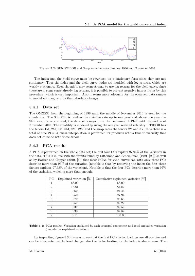
5.4. A PCA model for the yield curve and index
1998 2000 2002 2004 2006 2008 2010
1
2
3
4
5
6
7
8
Year
[%]
1M
2M
3M
6M
9M
12M
2Y
3Y
Figure 5.2: SEK STIBOR and Swap rates between January 1996 and November 2010.
The index and the yield curve must be rewritten on a stationary form since they are notstationary. Thus the index and the yield curve nodes are modeled with log returns, which areweakly stationary. Even though it may seem strange to use log returns for the yield curve, sincethese are in some sense already log returns, it is possible to prevent negative interest rates by thisprocedure, which is very important. Also it seems more adequate for the observed data sampleto model with log returns than absolute changes.
5.4.1 Data setThe OMXS30 from the beginning of 1996 until the middle of November 2010 is used for thesimulation. The STIBOR is used as the risk-free rate up to one year and above one year theSEK swap rates are used, the data set ranges from the beginning of 1996 until the middle ofNovember 2010. The volatility is modeled by using the one year realized volatility. STIBOR hasthe tenors 1M, 2M, 3M, 6M, 9M, 12M and the swap rates the tenors 2Y and 3Y, thus there is atotal of nine PCs. A linear interpolation is performed for products with a time to maturity thatdoes not coincide with these tenors.
5.4.2 PCA resultsA PCA is performed on the whole data set; the first four PCs explain 97.94% of the variation inthe data. This is in line with the results found by Litterman and Scheinkman (1991, [29]) as wellas by Barber and Copper (2010, [6]) that most PCAs for yield curves can with only three PCsdescribe more than 95% of the variation (notable is that by removing the index the first threefactors explains 97.68% of the variation). Notable is that the four PCs describe more than 95%of the variation, which is more than enough.
PC Explained variation [%] Cumulative explained variation [%]1 68.00 68.002 16.81 84.823 9.62 94.444 3.50 97.945 0.72 98.656 0.57 99.227 0.37 99.598 0.30 99.899 0.11 100.00
Table 5.1: PCA results: Variation explained by each principal component and total explained variation(cumulative explained variation).
By inspecting Figure 5.3 it is easy to see that the first PC’s factor loadings are all positive andcan be interpreted as the level change, also the factor loading for the index is almost zero. The
M. Hveem 55 (103)

Chapter 5. Modeling Financial Assets
OMXS30 1M 2M 3M 6M 9M 1Y 2Y 3Y−1
−0.8
−0.6
−0.4
−0.2
0
0.2
0.4
0.6
0.8
1
Risk Factor
Fac
tor
Load
ings
Principle Components
PC 1 (Level)
PC 2 (Steepness)
PC 3 (Index)
PC 4 (Curvature)
Figure 5.3: Factor loadings for the first four principle components, explaining changes in OMXS30 andthe yield curve up to three years.
second PC corresponds to steepness since its factor loadings change sign moving to longer tenors.The third PC corresponds to the index since the factor loading is close to one for OMXS30 andsmall for the rest of the factors. The fourth PC corresponds to curvature since products in themiddle tenors have positive factor loadings when the others have negative.
The factor loadings have been estimated during a period of approximately fifteen years. It isimportant that the factor loadings are stable through time if the distribution is used for sampling(since the estimation is used as a proxy for the future). To investigate if the model is adequatethe factor loadings and explanatory power of overlapping PCAs must be studied through timeand investigated for stability.
To conduct the study the data between January 1996 and June 2010 is divided into over-lapping three years intervals with a distance of six months. Thus this gives approximately 150observations, which is enough to retrieve a good estimation of the factor loadings.
The results are disclosed in Table 5.2, the first PC explains between 59% and 74% of thevariation and the other PCs exhibit similar patterns. On the other hand the total explanatorypower of the four PCs is always above 93.48%. Thus the four PCs explain most of the variationin the data sample regardless of which sample period selected. Notable is that the explanatorypower for the whole period was 97.94% and that the explanatory power in the model is higherduring the latter part of the time period. The PCA is computed on weekly returns in this section,performing the PCA on daily returns generates less stable results, with lower explanatory power.
The PCs’ factor loadings for the overlapping periods are disclosed in Figure 5.4. PC 1 has thesmallest variation, while the other three have higher levels of variation; the factor loadings havethe same structure for all samples. Concluded: the factor loadings are relative stable throughtime and stable enough to serve for simulation, even though the factor loadings exhibit somesample dependence.
5.4.3 Historical simulation
Historical simulation is a non-parametric model that draws samples from the empirical distri-bution with replacement. Thus to simulate new PCs; samples of factor scores should be drawnfrom the empirical distribution. This means sampling random dates (with equal probabilities)that are used to extract the corresponding factor scores, and replace the sample before the nextdraw. The advantage of using historical simulation is that the scenarios have happened in the
M. Hveem 56 (103)

5.4. A PCA model for the yield curve and index
Start End PC 1 PC 2 PC3 PC 4 Cumulative [%]Jan 1996 Dec 1998 73.51 11.18 9.74 3.09 97.52Jul 1996 Jun 1999 74.35 11.10 9.54 2.88 97.87Jan 1997 Dec 1999 67.34 11.71 10.47 3.99 93.51Jul 1997 Jun 2000 65.98 12.96 10.64 3.90 93.48Jan 1998 Dec 2000 65.80 12.96 10.74 4.08 93.59Jul 1998 Jun 2001 66.19 12.84 10.91 4.01 93.95Jan 1999 Dec 2001 64.59 14.88 11.30 3.69 94.46Jul 1999 Jun 2002 62.84 16.05 11.21 3.85 93.94Jan 2000 Dec 2002 67.95 17.38 9.75 2.91 98.00Jul 2000 Jun 2003 66.26 20.42 8.81 2.89 98.38Jan 2001 Dec 2003 65.79 21.01 8.64 2.99 98.43Jul 2001 Jun 2004 61.88 23.59 9.15 3.68 98.30Jan 2002 Dec 2004 58.80 24.77 9.00 4.53 97.10Jul 2002 Jun 2005 60.27 23.34 8.85 4.66 97.12Jan 2003 Dec 2005 61.38 21.96 9.17 4.59 97.09Jul 2003 Jun 2006 61.77 20.58 9.93 4.62 96.90Jan 2004 Dec 2006 62.62 19.84 10.16 4.44 97.07Jul 2004 Jun 2007 64.24 17.53 10.55 4.42 96.73Jan 2005 Dec 2007 63.68 18.51 10.66 4.52 97.37Jul 2005 Jun 2008 59.18 20.21 11.24 5.48 96.11Jan 2006 Dec 2008 69.61 20.96 7.58 1.20 99.35Jul 2006 Jun 2009 72.57 16.85 7.28 2.52 99.22Jan 2007 Dec 2009 71.42 17.58 7.09 2.70 98.79Jul 2007 Jun 2010 69.89 18.76 7.17 2.92 98.74Jan 1996 October 2010 68.00 16.81 9.62 3.50 97.94
Table 5.2: Variation explained by each principal component and total explained variation (cumulativeexplained variation) for 24 overlapping time periods between January 1996 and June 2010.
OMXS30 1M 2M 3M 6M 9M 1Y 2Y 3Y−1
−0.5
0
0.5
1
Risk Factor
Principle Component 1
Fac
tor
Lo
adin
gs
OMXS30 1M 2M 3M 6M 9M 1Y 2Y 3Y−1
−0.5
0
0.5
1
Risk Factor
Principle Component 2
Fac
tor
Lo
adin
gs
OMXS30 1M 2M 3M 6M 9M 1Y 2Y 3Y−1
−0.5
0
0.5
1
Risk Factor
Principle Component 3
Fac
tor
Lo
adin
gs
OMXS30 1M 2M 3M 6M 9M 1Y 2Y 3Y−1
−0.5
0
0.5
1
Risk Factor
Principle Component 4
Fac
tor
Lo
adin
gs
Figure 5.4: Factor loadings for the first four PCs for 24 overlapping time periods between January1996 and June 2010, each line corresponds to one sample.
M. Hveem 57 (103)

Chapter 5. Modeling Financial Assets
past, they are realistic and reflect the empirical distribution. Also it is really simple to implementand use historical simulation. On the other hand the problem is that there is no possibility ofimplementing new scenarios, thus the model is restricted to the outcomes of the past. This meansthat if no extreme events have happened in the past the probability of generating an extremescenario is zero. But the model is not restricted in this setup since the return over a three-yearperiod is generated from weekly returns. The model would be limited when studying only weeklyreturns, not yearly or monthly returns, thus simulating three-years returns using weekly datadoes not put any serious restrictions on the simulation.
The ith sample of the jth variable’s return using the first four PCs in a historical simulationis given as,
ri,j =
4∑k=1
QTk,jFi,k + εi,j ,
where,
εi,j ∼ N
(0,Var
[9∑k=5
QTk,jF•,k
]).
The sample should also be rescaled with its historical mean and standard deviation to attain thefinal sampled data.
5.4.4 Monte Carlo simulation
The idea of a Monte Carlo simulation is to fit a parametric distribution to the observed data;random samples are drawn from the parametric distribution to generate new data. Thus in thecase of the PCA a parametric distribution should be fitted to the observed factor scores.
By using QQ-plots, or other graphical illustrations such as histogram-fits and scatter plots,it is possible to illustrate and identify appropriate parametric distributions. It is easy to seethat the PCs can be described by t-distributions with different levels of freedom, location andscale, as shown in Figure 5.5. Scatter plots indicate that the four PCs come from a sphericaldistribution and that there exists dependence between the samples (scatter plots have ellipticalshapes) as seen in Figure 5.6.
t-location scalePC µ̂ σ̂ ν̂1 0.00 1.0296 2.41892 0.00 0.8880 4.17633 0.00 0.8189 8.87344 0.00 0.2976 2.7824
Table 5.3: The fit for a student’s t-distribution to each marginal distribution (factor scores) for thefirst four PCs attained through a maximum likelihood estimation.
Multivariate t-distribution
If ν (degrees of freedom) for the marginal distributions (in this case the individual PCs) are closeto each other it is possible to use a multivariate t-distribution, instead of using e.g. copulas. Arelative good fit is actually attained for this sample with a multivariate t-distribution, but it isnot as good as the t-copula model as disclosed further down. The following parameters for the
M. Hveem 58 (103)
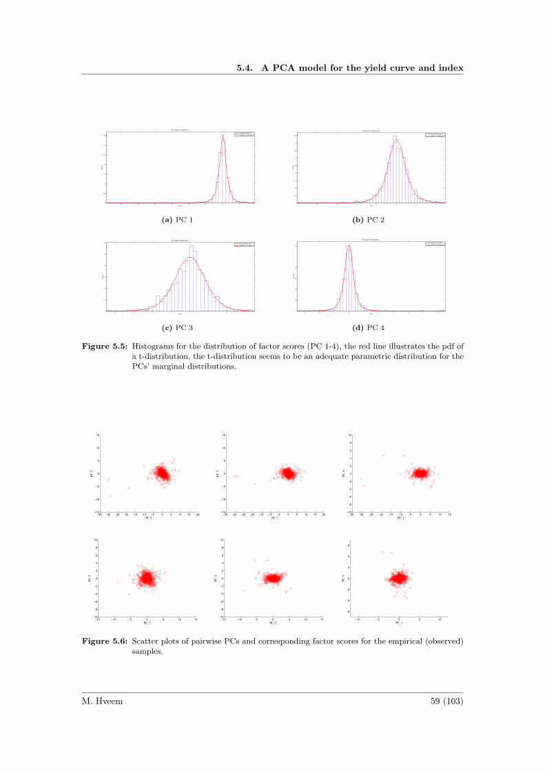
5.4. A PCA model for the yield curve and index
−30 −25 −20 −15 −10 −5 0 50
0.05
0.1
0.15
0.2
0.25
0.3
0.35
Data
Density
Principal Component 1
Factor Scores PC 1
Student’s t−distribution
(a) PC 1
−10 −8 −6 −4 −2 0 2 40
0.05
0.1
0.15
0.2
0.25
0.3
0.35
0.4
0.45
Data
Density
Principal Component 2
Factor Scores PC 2
Student’s t−distribution
(b) PC 2
−4 −3 −2 −1 0 1 2 30
0.1
0.2
0.3
0.4
0.5
0.6
Data
Density
Principal Component 3
Factor Scores PC 3
Student’s t−distribution
(c) PC 3
−3 −2 −1 0 1 2 3 4 5 60
0.2
0.4
0.6
0.8
1
1.2
Data
Density
Principal Component 4
Factor Scores PC 4
Student’s t−distribution
(d) PC 4
Figure 5.5: Histograms for the distribution of factor scores (PC 1-4), the red line illustrates the pdf ofa t-distribution, the t-distribution seems to be an adequate parametric distribution for thePCs’ marginal distributions.
−35 −30 −25 −20 −15 −10 −5 0 5 10 15 20−15
−10
−5
0
5
10
15
PC 1
PC
2
−35 −30 −25 −20 −15 −10 −5 0 5 10 15 20−15
−10
−5
0
5
10
15
PC 1
PC
3
−35 −30 −25 −20 −15 −10 −5 0 5 10 15−10
−8
−6
−4
−2
0
2
4
6
8
10
PC 1
PC
4
−15 −10 −5 0 5 10 15−10
−8
−6
−4
−2
0
2
4
6
8
10
PC 2
PC
3
−15 −10 −5 0 5 10 15−10
−8
−6
−4
−2
0
2
4
6
8
10
PC 2
PC
4
−10 −5 0 5 10
−6
−4
−2
0
2
4
6
PC 3
PC
4
Figure 5.6: Scatter plots of pairwise PCs and corresponding factor scores for the empirical (observed)samples.
M. Hveem 59 (103)

Chapter 5. Modeling Financial Assets
multivariate t-distribution are attained using a maximum likelihood estimation,
µ̂ =
0000
, Σ̂ =
2.337 0 0 0
0 0.5770 0 00 0 0.3301 00 0 0 0.1201
, ν̂ = 3.2326.
It is common to assume that the residual term is multivariate normal distributed. This is not anecessary condition and the residual term ε can be rewritten as a matrix (factor loadings) timesa stochastic vector (vector of the remaining PCs). For the observed data set the stochastic vectoris approximately multivariate t-distributed. Thus,
ri,j =
4∑k=1
QTk,jFi,k +
9∑k=5
QTk,jF
εi,k, (5.1)
where,
F ∼ tν (0,Σ) , Fε ∼ tνε (0,Σε) ,
and,
Σ̂ε =
0.0195 0 0 0 0
0 0.0154 0 0 00 0 0.0099 0 00 0 0 0.0082 00 0 0 0 0.0030
, ν̂ε = 2.8622.
Hence to perform a Monte Carlo simulation, using a multivariate t-distribution (in this setting),draw samples of F and Fε and plug in the sampled values into Equation 5.1 above. The multi-variate t-distribution is a normal variance mixture and hence easy to sample from e.g. MATLABhas an inbuilt function to perform the operation.
Copula
The marginal distributions for the factor scores are approximately t-distributed as seen above.Thus by using a Copula it is possible to maintain the marginal distributions intact and use thedependence structure from another distribution. Thus an adequate choice is to use t-marginalsand a t-copula since the dependence structure is spherical and similar to the one sampled froma t-copula. If all the marginals had the same levels of freedom it would be the exact same modelas with a multivariate t-distribution, but as seen in Table 5.3 this is not the case. The marginalsdescribed in Table 5.3 will be used for the first four PCs.
The best fit (using MATLAB’s copulafit) is a t-copula with ν̂ = 3.0617, which has thefollowing dependence structure,
ρ̂ =
1.0000 −0.4985 −0.2170 0.1680−0.4985 1.0000 −0.0841 0.0733−0.2170 −0.0841 1.0000 0.12020.1680 0.0733 0.1202 1.0000
.
To sample from the copula with t-marginals sample from a multivariate t-distribution withν̂ = 3.0617 as above, use the cumulative distribution for a univariate tν̂ variable on the sample,the samples are now uniformed samples from the tν̂ copula. Take the inverse of each cumulativemarginal distribution on the samples to attain the new centered and rescaled samples, multiplythese samples with each dispersion coefficient and add the mean to attain the final factor scoresample.
M. Hveem 60 (103)

5.4. A PCA model for the yield curve and index
−35 −30 −25 −20 −15 −10 −5 0 5 10 15 20−15
−10
−5
0
5
10
15
PC 1
PC
2
−35 −30 −25 −20 −15 −10 −5 0 5 10 15 20−15
−10
−5
0
5
10
15
PC 1
PC
3
−35 −30 −25 −20 −15 −10 −5 0 5 10 15−10
−8
−6
−4
−2
0
2
4
6
8
10
PC 1
PC
4
−15 −10 −5 0 5 10 15−10
−8
−6
−4
−2
0
2
4
6
8
10
PC 2
PC
3
−15 −10 −5 0 5 10 15−10
−8
−6
−4
−2
0
2
4
6
8
10
PC 2
PC
4
−10 −5 0 5 10
−6
−4
−2
0
2
4
6
PC 3
PC
4
Figure 5.7: Scatter plots of pairwise PCs and corresponding factor scores sampled from the multivariatet-distribution.
The error term can be modeled either through a multivariate t-distribution or any otherparametric distribution such as a copula model. It does not matter a lot which distribution ischosen since the error explains the remaining noise in the data (which is small, less than 2.5%of the total variance). By fitting a t-copula with t-marginals the following result is retrieved,
t-location scalePC µ̂ σ̂ ν̂5 0.00 0.1405 2.87716 0.00 0.1080 2.58977 0.00 0.0808 2.49638 0.00 0.0832 2.68729 0.00 0.0692 3.8576
Table 5.4: Parameters for the residual factor scores attained through a maximum likelihood estimationof t-distributions.
ρ̂ε =
1.0000 0.0658 0.1179 0.1837 0.11330.0658 1.0000 0.1380 0.1260 −0.01830.1179 0.1380 1.0000 0.2901 0.16610.1837 0.1260 0.2901 1.0000 0.13380.1133 −0.0183 0.1661 0.1338 1.0000
, ν̂ε = 3.4124.
Figure 5.9 shows that the copula provides a much better fit for the marginals than the multi-variate t-distribution. The copula provides also a better dependence structure, when comparingFigure 5.7 and 5.8 with Figure 5.6. Thus it is easy to conclude from the plots that the copulaprovides a better fit, notable is that the multivariate t-distribution does not provide a bad fit atall, just not as good as the copula model.
M. Hveem 61 (103)

Chapter 5. Modeling Financial Assets
−35 −30 −25 −20 −15 −10 −5 0 5 10 15 20−15
−10
−5
0
5
10
15
PC 1
PC
2
−35 −30 −25 −20 −15 −10 −5 0 5 10 15 20−15
−10
−5
0
5
10
15
PC 1
PC
3
−35 −30 −25 −20 −15 −10 −5 0 5 10 15−10
−8
−6
−4
−2
0
2
4
6
8
10
PC 1
PC
4
−15 −10 −5 0 5 10 15−10
−8
−6
−4
−2
0
2
4
6
8
10
PC 2
PC
3
−15 −10 −5 0 5 10 15−10
−8
−6
−4
−2
0
2
4
6
8
10
PC 2
PC
4
−10 −5 0 5 10
−6
−4
−2
0
2
4
6
PC 3
PC
4
Figure 5.8: Scatter plots of pairwise PCs and corresponding factor scores sampled from the t-copulawith t-marginals.
Hence an appropriate choice is to use either the copula model with Monte Carlo simulation orhistorical simulation, the result does not differ a lot in practice. This is particularly the case sinceweekly return data is used to simulate three years trajectories. The two models would differ muchmore if the return for just one week should be simulated. When sampling one week’s data onlyone draw is required, thus limiting the outcomes to the empirical distribution. When samplingthree-years returns from weekly returns it is still possible to generate almost an infinite numberof combinations using the empirical distribution, 156 return samples with replacement out of 781observed weeks provides 781156 different combinations, which converges towards infinity.
The advantage of using historical simulation instead of the parametric simulation is that itis much faster to use, reducing the sample time in many cases from several hours to minutes.Thus a historical simulation is used further in this thesis since a sensitivity analysis shows thatthe results are in practice identical using both.
M. Hveem 62 (103)
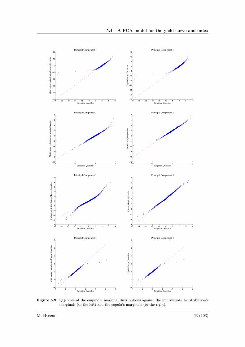
5.4. A PCA model for the yield curve and index
−35 −30 −25 −20 −15 −10 −5 0 5 10−50
−40
−30
−20
−10
0
10
20
Empirical Quantiles
Mu
ltiv
aria
te t
−d
istr
ibu
tio
n M
arg
in Q
uan
tile
sPrincipal Component 1
−35 −30 −25 −20 −15 −10 −5 0 5 10−35
−30
−25
−20
−15
−10
−5
0
5
10
15
Empirical Quantiles
Co
pu
la M
arg
in Q
uan
tile
s
Principal Component 1
−10 −5 0 5−10
−8
−6
−4
−2
0
2
4
6
8
Empirical Quantiles
Mu
ltiv
aria
te t
−d
istr
ibu
tio
n M
arg
in Q
uan
tile
s
Principal Component 2
−10 −5 0 5−12
−10
−8
−6
−4
−2
0
2
4
6
Empirical Quantiles
Co
pu
la M
arg
in Q
uan
tile
s
Principal Component 2
−5 −4 −3 −2 −1 0 1 2 3 4−5
−4
−3
−2
−1
0
1
2
3
4
5
Empirical Quantiles
Mu
ltiv
aria
te t
−d
istr
ibu
tio
n M
arg
in Q
uan
tile
s
Principal Component 3
−5 −4 −3 −2 −1 0 1 2 3 4−5
−4
−3
−2
−1
0
1
2
3
4
Empirical Quantiles
Co
pu
la M
arg
in Q
uan
tile
s
Principal Component 3
−4 −2 0 2 4 6 8−4
−2
0
2
4
6
8
Empirical Quantiles
Mu
ltiv
aria
te t
−d
istr
ibu
tio
n M
arg
in Q
uan
tile
s
Principal Component 4
−4 −2 0 2 4 6 8−4
−2
0
2
4
6
8
Empirical Quantiles
Co
pu
la M
arg
in Q
uan
tile
s
Principal Component 4
Figure 5.9: QQ-plots of the empirical marginal distributions against the multivariate t-distribution’smarginals (to the left) and the copula’s marginals (to the right).
M. Hveem 63 (103)


CHAPTER 6
Portfolio Optimization
The fund should yield a high return as well as limit the risk under CVaR. CVaR is used as riskmeasure since the distribution of the structured products is skewed and exhibits kurtosis, thusrisk measures such as standard deviation are inappropriate (as described earlier). In this chapter,the fund is allowed to rebalance the portfolio every quarter, the investment horizon is three years,the fund is allowed to allocate a maximum of 30% in each asset, CVaR will be considered forα = 0.95. All structured products in this chapter are 100% capital guaranteed and follows thedynamics given in Chapter 3, thus the structured products have a time to maturity of three yearsat issuance, the bond’s notional amount equals the price of the underlying, the strike as well asthe price of the product itself at issuance.
Only proportional transaction costs are considered since fixed transaction costs transformsthe linear CVaR optimization problem into a mixed integer linear problem, which increases thecomplexity of the problem a lot.
The chapter covers three different types of portfolio choices: fixed portfolio weights, rollingportfolio weights and dynamic portfolio weights. The different alternatives are evaluated inrelation to a benchmark fund and the most beneficial fund construction is investigated. Theresults indicate that the most beneficial setup is the dynamic portfolio weights scheme, where amodified Korn and Zeytun framework is proposed. The study indicates that the most imperativefactor that affects the return is in fact not the portfolio selection itself but instead the transactioncosts.
The first portfolio allocation strategy/scheme that is described is the fixed portfolio weightstrategy.
6.1 Fixed portfolio weights
Fixed portfolio weights is the setup where product one always is the product closest to maturityand product twelve the product with the longest time to maturity (since it exists only twelveproducts), thus it is similar to the portfolios used in Section 4.3, where there is always twelvecapital guaranteed structured products available. The portfolio will be allocated using the CVaRalgorithm described in Chapter 2 with the modification that no binary variables will be used (nofixed transaction costs), since they turn the problem into a mixed integer linear problem, whichis not desirable. The return is used as target function since this problem is better defined thanhaving the return as a constraint (needs less iterations via the simplex method). Since the fixedweights concept is used, which is a relative theoretical concept, it is interesting to investigatewhich products are more optimal than others to allocate in, when considering tenors. Thus thestudy disregards transaction costs initially to investigate the optimal choice in a perfect marketsetting. The result should be seen as a guideline for optimal portfolio choice, i.e. which types ofproducts that are better to invest in than others, regarding the tenor.
The results presented in Section 4.3 are in line with the results found in this section. Theproducts closest to maturity are associated with the highest risk, i.e. CVaR, where it was previ-ously found that the products closest to maturity have the worst outcomes of equivalent option
65

Chapter 6. Portfolio Optimization
portfolios. Investing in the products closest to maturity imposes an “all or nothing situation”for the options, while retrieving a more smooth return distribution for newly issued products asproven earlier (even though the interest rate was ignored in the previous chapters). Since similarresults are retrieved when including the effect of interest rate changes (as seen in Table 6.1) theassumption that the risk of movements in the underlying is the most prevalent risk factor canbe confirmed. Notable is that the expected return is higher for products with higher risk, thus itseems to be adequate to use a CVaR optimization scheme to attain a smooth efficient frontier.The analysis is performed via 100,000 six-year trajectory samples based on the model describedin Chapter 5. The return over the last three years of each sample trajectory is considered, sincethe first three years are needed to generate relevant price data as the price process is path depen-dent. The last three years observed price data on the market is not used as start data since theanalysis should be conducted independent of the current market. Instead different start levelsfor the yield curve will be considered, i.e. the yield curve that is in the beginning of the six-yearperiod. In this section, the yield curve as of 15th November 2010, representing a low yield casewill be used. In the appendix the case with an arbitrary yield curve is disclosed. The results arein general the same, mostly imposing just higher expected return and risk.
It is important to understand that the result may not look exactly the same for all markets.It is also important to notice that a more general concept is investigated in this section since theprevious three-year trajectories are simulated. Thus the efficient frontier would look differentif an investor would want to invest in structured products today since the current yield curve,index level, strikes and participation rates are known. Hence the results in this chapter aremainly general results, i.e. in the long run the efficient frontiers etc. would look like this, notnecessary all the time.
Thus the hypothesis that was presented in Section 4.3 was correct, the highest risk is associ-ated with products that are closest to maturity and the newly issued products have a lower riskas disclosed in Table 6.1. Thus it is reasonable to assume that the investment strategy proposedearlier in Chapter 4 is still adequate.
2 4 6 8 10 12 14 1616.5
17
17.5
18
18.5
19
19.5
20
Efficient Frontier Fixed Portfolio Weights
Portfolio CVaRα = 0.95
[%]
Expec
ted P
ort
foli
o R
eturn
[%
]
Figure 6.1: Efficient frontier for the optimization choice using the fixed portfolio weights setting, α =0.95.
The CVaR algorithm described in Chapter 2 is applied to produce a robust efficient frontier;the result is disclosed in Figure 6.1. Transaction costs have been disregarded and the restrictionthat it is only allowed to invest a maximum of 30% in each asset is in place. Since the optimizationis computer intensive, it is not possible to use a lot more than approximately 1,000 scenariosfor the efficient frontier (in a timely manner on a regular PC). Thus to attain robust results100 efficient frontiers are simulated for different risk levels (CVaR) as constraint and the averageof these weights are calculated to attain robust portfolio weights. Thus yielding a more robustefficient frontier, which reflects the intrinsic frontier in a better manner.
Figure 6.1 indicates that the expected return increases as the risk increases, and the frontier
M. Hveem 66 (103)

6.1. Fixed portfolio weights
is quite similar the frontier for a classic Markowitz optimization problem with standard deviationas risk measure.
Product Number, CVaR0.95 [%]1 2 3 4 5 6 7 8 9 10 11 12
18.46 14.88 12.41 10.52 9.33 8.04 7.08 6.40 4.68 4.23 3.92 3.74Product Number, Expected return [%]
1 2 3 4 5 6 7 8 9 10 11 1220.14 19.71 19.63 19.07 18.12 17.71 17.30 16.93 16.48 16.14 15.81 15.51
Table 6.1: The table describes the CVaR at the 95% confidence level and expected return for thedifferent products over the three-year period using the fixed portfolio weights setting.
Next the sensitivity of each scenario’s portfolio weights is analyzed. It is important to analyzethe standard deviation of the portfolio weights, since it discloses how robust the weights are, andif it is necessary to use multiple samples to attain a representative solution to the optimizationproblem. 100 samples of 1,000 scenarios for three different levels of CVaR are used, one low risk,one medium risk and one high-risk level. The portfolio weights are approximately equally robustfor the low risk scenarios and for high-risk scenarios, with slightly more robust portfolio weightsfor the high-risk level, as Table 6.2 indicates.
Weights, standard deviation [%]CVaR0.95 1 2 3 4 5 6 7 8 9 10 11 12
4% 0.80 0.95 8.69 9.7 0.04 5.25 8.82 10.67 9.07 11.03 11.94 10.068% 6.42 7.37 5.50 6.91 3.73 8.01 9.00 11.05 8.01 7.69 6.37 4.9512% 9.75 9.94 1.80 5.73 2.62 3.72 2.47 3.92 1.57 1.11 0.39 0.50
Table 6.2: The table describes the robustness (standard deviation) of the weights for a portfolio al-location using 1,000 scenarios and for three different CVaR levels using the fixed portfolioweights setting.
The sensitivity of the portfolio weights is higher with less sample scenarios. Also it is moreadequate to use CVaR as a constraint and maximizing the return as the target, than the otherway around, since it does not only require less iterations but also generates more stable portfolioweights. Table 6.2 shows that there exists significant standard deviation for the portfolio weights.So what does this imply? Since each sample has different paths up till the start of investment ahigh standard deviation implies that it is important to not use a generalized allocation scheme,since the weights shift much depending on the scenarios.
From the distribution and CVaR results for the individual products it is reasonable to assumethat lower levels of CVaR allocate most of the capital to the products with the longest time tomaturity (which is the case). But as the maximum CVaR allowed increases the portfolio willallocate in shorter products to yield a higher expected return (since the expected return increasesalmost linear over the twelve assets). Thus the frontier portfolios (weights), disclosed in Figure6.2, are attained.
Hence depending on the desired maximum risk level the portfolio weights should be chosenaccording to Figure 6.2 and the portfolio would receive the expected return according to Figure6.1.
Thus following the path of capital guarantee; a fund should allocate mainly in the last four- five products to minimize the CVaR for the portfolio. It should also, depending on its risktolerance (and transaction costs), sell of assets after a number of quarters elapsed. The risklevel and expected return will be very dependent on the transaction costs, which is importantto notice. Consider transaction costs of 2% (2% in proportional transaction costs each timethe fund sells or buys an asset) and a portfolio which holds equal weights in the longest tenorsw9 = w10 = w11 = w12. The portfolio has without transaction costs a CVaR0.95 of 3.62% and
M. Hveem 67 (103)

Chapter 6. Portfolio Optimization
4.2 5.2 6.2 7.2 8.2 9.2 10.2 11.2 12.2 13.2 14.20
10
20
30
40
50
60
70
80
90
100
Wei
ght
[%]
Portfolio CVaRα = 0.95
[%]
w1
w2
w3
w4
w5
w6
w7
w8
w9
w10
w11
w12
Figure 6.2: Portfolio weights for the efficient frontier using the fixed portfolio weights setting, α = 0.95.
an expected return of 15.98% over three years. Including the transaction costs it will have aCVaR0.95 of 9.29% and an expected return of 9.16%. On the other hand a portfolio holdingequal amounts invested in products twelve throughout seven has a CVaR0.95 of 7.52% and anexpected return of 11.75% including the transaction cost. Thus the problem must be modifiedto find a solution including transaction costs.
To solve how to allocate in an optimal way, including transaction costs, an alternative CVaRalgorithm with proportional transaction costs is introduced, which can approximate the inducedtransaction costs of a portfolio with fixed weights. The weight held in asset 12 one quarter isapproximately held in asset 11 the next quarter and so on. Thus the fund can, by solving the opti-mization problem below, attain portfolio weights that are desirable when taking in considerationtransaction costs.
maxw,w+,w−,z,β
1
S
S∑k=1
(1 +RwT,k
),
such that:
β +1
S (1− α)
S∑k=1
zk ≤ C,
1 +RwT,k =(1 +R1
T,k
)w1 + ...+
(1 +RNT,k
)wN , k = 1, ..., S
RwT,k + β + zk ≥ 0, k = 1, ..., S
zk ≥ 0, k = 1, ..., S
N∑i=1
wi +
N−1∑i=1
(TC+
i w+i + TC−i w
−i
)+ TC+
NwN = 1,
wi = wi+1 + w+i − w
−i , i = 1, ..., N − 1
wN = w1 + w+N − w
−N
wi ≥ 0, w±i ≥ 0, i = 1, ..., N
The optimal portfolio weights are investigated for the cases of no transaction costs and threedifferent levels of transaction costs, when minimizing the CVaR, given a positive return. Theoptimal weights are investigated in a setting of a low initial yield curve and the setting of anarbitrary, random start yield curve, the results are disclosed in Figure 6.3. It is in general most
M. Hveem 68 (103)
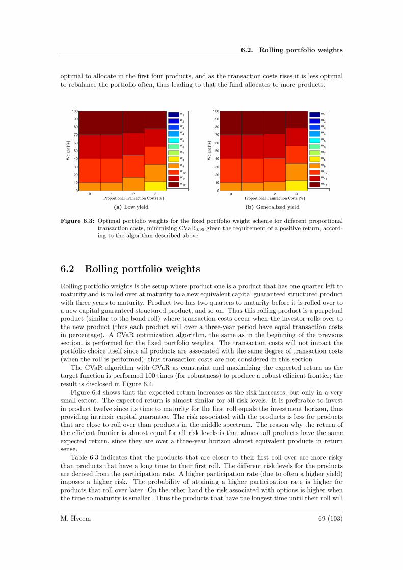
6.2. Rolling portfolio weights
optimal to allocate in the first four products, and as the transaction costs rises it is less optimalto rebalance the portfolio often, thus leading to that the fund allocates to more products.
0 1 2 30
10
20
30
40
50
60
70
80
90
100
Wei
gh
t [%
]
Proportional Transaction Costs [%]
w
1
w2
w3
w4
w5
w6
w7
w8
w9
w10
w11
w12
(a) Low yield
0 1 2 30
10
20
30
40
50
60
70
80
90
100
Wei
gh
t [%
]
Proportional Transaction Costs [%]
w
1
w2
w3
w4
w5
w6
w7
w8
w9
w10
w11
w12
(b) Generalized yield
Figure 6.3: Optimal portfolio weights for the fixed portfolio weight scheme for different proportionaltransaction costs, minimizing CVaR0.95 given the requirement of a positive return, accord-ing to the algorithm described above.
6.2 Rolling portfolio weights
Rolling portfolio weights is the setup where product one is a product that has one quarter left tomaturity and is rolled over at maturity to a new equivalent capital guaranteed structured productwith three years to maturity. Product two has two quarters to maturity before it is rolled over toa new capital guaranteed structured product, and so on. Thus this rolling product is a perpetualproduct (similar to the bond roll) where transaction costs occur when the investor rolls over tothe new product (thus each product will over a three-year period have equal transaction costsin percentage). A CVaR optimization algorithm, the same as in the beginning of the previoussection, is performed for the fixed portfolio weights. The transaction costs will not impact theportfolio choice itself since all products are associated with the same degree of transaction costs(when the roll is performed), thus transaction costs are not considered in this section.
The CVaR algorithm with CVaR as constraint and maximizing the expected return as thetarget function is performed 100 times (for robustness) to produce a robust efficient frontier; theresult is disclosed in Figure 6.4.
Figure 6.4 shows that the expected return increases as the risk increases, but only in a verysmall extent. The expected return is almost similar for all risk levels. It is preferable to investin product twelve since its time to maturity for the first roll equals the investment horizon, thusproviding intrinsic capital guarantee. The risk associated with the products is less for productsthat are close to roll over than products in the middle spectrum. The reason why the return ofthe efficient frontier is almost equal for all risk levels is that almost all products have the sameexpected return, since they are over a three-year horizon almost equivalent products in returnsense.
Table 6.3 indicates that the products that are closer to their first roll over are more riskythan products that have a long time to their first roll. The different risk levels for the productsare derived from the participation rate. A higher participation rate (due to often a higher yield)imposes a higher risk. The probability of attaining a higher participation rate is higher forproducts that roll over later. On the other hand the risk associated with options is higher whenthe time to maturity is smaller. Thus the products that have the longest time until their roll will
M. Hveem 69 (103)

Chapter 6. Portfolio Optimization
3 4 5 6 7 8 917.8
17.81
17.82
17.83
17.84
17.85
17.86
17.87
17.88
Efficient Frontier Rolling Portfolio Weights
Portfolio CVaRα = 0.95
[%]
Expec
ted P
ort
foli
o R
eturn
[%
]
Figure 6.4: Efficient frontier for the optimization choice using the rolling portfolio weights setting,α = 0.95.
risk receiving higher participation rates in the end, but they will only go through a few quarters(the ones with the least risk) until the investment horizon ends with this high participation rate.Also these products will benefit of the previous roll before the high participation rate that witha high probability had a low participation rate. Thus the average participation rate over theinvestment horizon is higher for products with 1-9 quarters to the next roll, imposing a higherrisk. The risk levels and expected returns for the twelve different rolls are given in Table 6.3.
Product (months until next roll), CVaR0.95 [%]1 2 3 4 5 6 7 8 9 10 11 12
9.28 10.57 11.43 10.63 10.68 10.31 9.73 9.12 8.15 6.86 5.06 0.00Product (months until next roll), Expected return [%]
1 2 3 4 5 6 7 8 9 10 11 1218.04 18.01 17.98 17.57 17.57 17.54 17.58 17.60 17.64 17.69 17.72 17.81
Table 6.3: The table describes the CVaR at the 95% confidence level and expected return for thedifferent products over the three-year period for the different rolls.
The robustness of the weights is also studied through investigating the standard deviationsof the weights as previously, the result is presented in Table 6.4.
Weights, standard deviation [%]CVaR0.95 1 2 3 4 5 6 7 8 9 10 11 12
4% 9.35 11.65 7.86 5.89 4.32 4.83 2.98 2.78 6.59 8.34 10.44 4.726% 12.76 12.19 10.43 7.94 7.89 7.22 5.86 5.05 12.66 13.40 11.89 12.308% 12.25 11.83 9.89 7.95 8.71 7.77 8.69 5.62 13.87 13.73 12.03 12.34
Table 6.4: The table describes the robustness (standard deviation) of the weights for a portfolio allo-cation using 1,000 scenarios and for three different CVaR levels using the rolling portfolioweights setting.
The standard deviation result is similar to the result in the previous section, which indicatesthat it is important as a portfolio manager to not use a generalized scheme for the allocation ofthe portfolio since the portfolio weights depends a lot on the previous path.
Investigating the portfolio weights for the robust efficient frontier shows that the portfolioshould, to attain lower levels of CVaR, allocate to the products that have a lower individualCVaR, which is reasonable as disclosed in Figure 6.5.
The expected return will in the long run be very similar for all rolls, while the risk profile of
M. Hveem 70 (103)

6.3. Benchmark fund
4.6 5.6 6.6 7.6 8.60
10
20
30
40
50
60
70
80
90
100
Wei
gh
t [%
]
Portfolio CVaRα = 0.95
[%]
w1
w2
w3
w4
w5
w6
w7
w8
w9
w10
w11
w12
Figure 6.5: Portfolio weights for the efficient frontier using the rolling portfolio weights setting, α =0.95.
the products differs. Thus it is better to invest in products with a long time to the next roll. Thehigh standard deviation of the portfolio weights implies that it is very important to evaluate theportfolio depending on the observed paths (yield curve, participation rate, index level etc) sincethey will impact both the expected return and the risk profile.
Thus when investing with the rolling weight scheme, it is better to allocate to the newly issuedproducts (as stated in the previous chapters and sections). It is better to invest with rollingportfolio weights than the fixed weight scheme if the expected return it yields is satisfactory.Thus by requiring a maximum of 3.80% in CVaR0.95 the portfolio will actually have an expectedreturn of 17.82% over three years (excluding transaction costs, which would increase the CVaRand decrease the expected return), compared to the fixed weights which only yields an expectedreturn of 16.88% for the same risk level, which also induces much higher transaction costs.
As described earlier in this paper, a portfolio’s risk and return is only relevant in a certaincontext, thus it is imperative that the different portfolio constructions are compared with abenchmark fund.
6.3 Benchmark fund
The analysis would be less relevant without a comparison with a relevant benchmark. Observedmarket data for the Swedish market has been used throughout the analysis in this chapter,thus the SPF must be benchmarked against alternatives at the Swedish market. Consider thebenchmark fund described earlier, which places 30% of its capital in the index, plus minus 10%,and the rest of the capital in a basket of bonds with time to maturity between three months tothree years (approximately equally weighted, rolling). This yields an expected return, over thethree years investment horizon, of 19.81% including the expectation of 3% annual dividends inthe index and a CVaR0.95 of 9.49%. The distribution of the fund returns is given in Figure 6.6.When disregarding the expectation of the dividends the portfolio instead receives an expectedreturn of 16.12% and a CVaR0.95 of 10.75%.
Thus the distributions of the two, with or without dividend, are of course almost identical,the only thing that differs is approximately a parallel shift. The results indicate that it is hardfor the SPF to compete with the benchmark fund including dividends (in terms of return) sincethe benchmark has a much higher expected return given the same risk level. Thus the SPFmust compete with the benchmark portfolio given low risk. In Table 6.5 results for differentbenchmark funds are disclosed. Notable is that transaction costs have been disregarded, whichwould decrease the expected return of these products.
M. Hveem 71 (103)

Chapter 6. Portfolio Optimization
−0.5 0 0.5 1 1.5 2 2.50
100
200
300
400
500
600
700
Benchmark Fund
CVaR0.95
= 9.49%
(a) Incl. dividend
−0.5 0 0.5 1 1.5 2 2.50
50
100
150
200
250
300
350
400
450
Benchmark Fund
CVaR0.95
= 10.75%
(b) Excl. dividend
Figure 6.6: Histograms over the sampled three-year returns for the benchmark fund, εbench = 0.3.
Incl. Dividends. Excl. Dividends.Index allocation Expected Return CVaR0.95 Expected Return CVaR0.95
10% 11.40 -1.66 10.16 -1.2020% 15.43 3.25 13.05 4.3830% 19.50 8.72 16.12 10.7540% 23.88 14.35 19.16 17.13
Table 6.5: The table discloses the expected return and CVaR for different levels of index weights overthe three-year period for a benchmark fund.
Table 6.1, 6.3 and 6.5 indicate that the SPF can compete initially (without transaction costs)in the low risk spectrum, where the rolling weights portfolio generates higher expected returnsrelative to the risk, which is also the case for the fixed portfolio weights. Thus these types offunds would be able to compete with the benchmark fund in the low risk spectrum. This is alsoin line with the idea of the SPF, which is that it should be a low risk fund, and the results showthat it is only possible for the SPF to compete against other low risk funds to yield a higherexpected return.
The next section will investigate the last allocation scheme, the dynamic portfolio weightsallocation scheme.
6.4 Dynamic portfolio weights
The allocation problem is quite complex for the SPF. It is assumed that product one is theproduct with one quarter until maturity, product two is the product with two quarters untilmaturity and so on as previously, hence there exists twelve products (the products are alsostandard). The fund manager has the possibility today to invest in twelve structured products,where only one of the products does not mature before the end of the investment horizon. Thuswhen considering to allocate the portfolio over a three-year period the fund manager needs totake in count how the payoff of the products that mature before the end of the investmenthorizon should be reinvested. It is necessary to consider the full three-year time horizon sincea portfolio allocated on a three-month basis would be suboptimal and induce high transactioncosts. Thus it is desirable to investigate the portfolio choice for the whole three-year time periodto avoid excessive transaction costs (since this is the time to maturity of the longest product thatexists). Korn and Zeytun (2009, [27]) propose a method to solve optimal investment problemswith structured products under CVaR constraints, where the investor’s investment horizon islonger than the time to maturity. Korn and Zeytun proposes the following modified multiple
M. Hveem 72 (103)

6.4. Dynamic portfolio weights
period CVaR allocation algorithm,
maxw,ν,z,β
1
S
S∑k=1
Rw,νT,k ,
such that:
Rw,νT,k = w1R1,νT,k + ...+ wN−1R
N−1,νT,k + wNR
NT,k, k = 1, ..., S
Rj,νT,k =(
1 + Πjk
) [νjj+1
(1 + rj+1
T−j,k
)+ ...+ νjN
(1 + rNT−j,k
)]− 1, j = 1, ..., N − 1
Rw,νT,k + β + zk ≥ 0, k = 1, ..., S
β +1
S (1− α)
S∑k=1
zk ≤ C,
zk ≥ 0, k = 1, ..., S
w1 + ...wN = 1,
wi ≥ 0, i = 1, ..., N
νj ≥ 0, j = 1, ..., N − 1
where νjl is the percentage of the product j’s payoff that is allocated to asset l after maturity,rlT−j,k is the return of asset l for the remaining time period (time until the end of the investmenthorizon from time j), Πj
k is the return of asset j from the start of the investment period untilits maturity and k corresponds to the scenario. Thus each product that matures is reinvestedusing the weights νjl . Note that the last product does not mature prior to the investment horizonthus RNT,k = ΠN
k . The optimization problem above is without transaction costs, the proportionaltransaction costs constraints and budget constraints can be added in the exact same way as forthe regular CVaR optimization problem.
The problem with this setting is that it is no longer a linear optimization problem. Thusit cannot be solved with only a simplex procedure. It must instead be solved by creating op-timization loops, where each intermediate rebalancing point creates a new loop. Eleven outeroptimization loops, with twelve possible products to allocate within, are needed since the portfo-lio has eleven intermediate rebalancing points. It is not feasible to allocate with this sophisticatedoptimization algorithm in this setting since the time to attain a solution would be months, notminutes or hours, and for robust weights it would take years to solve the optimization problem.Also, the optimization problem is not always convex, thus resulting in different solutions, givendifferent start values in the optimization.
6.4.1 Modifying the Korn and Zeytun framework
The algorithm described by Korn and Zeytun is adequate for a limited number of intermediatetime periods, thus relative few assets, since the iterations and as a consequence the comput-ing time grows exponentially. Concluded: it is not possible to use this algorithm to solve theallocation problem in this setting.
The optimization problem is modified by setting constraints on νjl , such that the problem iseasier to solve. Let νjl be the weights that minimize the CVaR for the particular product j includ-ing the reinvestment, thus reducing the total problem to only solving twelve linear optimizationproblems.
Thus the modified algorithm is as follows,
M. Hveem 73 (103)

Chapter 6. Portfolio Optimization
i. Sample N trajectories from the model described in Chapter 5 to attain returns forthe structured products.
ii. Solve the CVaR optimization problem with minimizing CVaR as target and the con-straint of a positive return for the period between N − 1 to N to attain νN−1,rN−1T−(N−2),k and complete the full return trajectory for product N − 1.
iii. Repeat ii until the full price trajectories for all products are known, thus betweenN − 2 to N , N − 3 to N and so on (in this case eleven optimization problems).
iv. Solve the well-defined CVaR optimization problem between 1 and N to attain initialweights w (since all scenario trajectories are known).
v. Repeat steps i - iv 100 times to attain robust portfolio weights.
The results attained through this allocation scheme are much more beneficial than the pre-vious two allocation schemes. Thus it is this allocation scheme that should be used in relationto the benchmark portfolio, since it can generate higher expected returns to the same risk level.Without taking in count transaction costs the robust efficient frontier in Figure 6.7 is attained.
3 3.5 4 4.5 5 5.5 6 6.5 7 7.5 817.45
17.46
17.47
17.48
17.49
17.5
17.51
17.52
17.53
Efficient Frontier Dynamic Portfolio Weights
Portfolio CVaRα = 0.95
[%]
Expec
ted P
ort
foli
o R
eturn
[%
]
Figure 6.7: Efficient frontier for the optimization choice using the dynamic portfolio weights and themodified Korn and Zeytun framework, α = 0.95.
The expected return does not increase a lot as the portfolio increases its risk tolerance, moststructured products in this setting have similar expected returns. Most of the reinvested capitalwill be placed in the newly issued product, since the products with the longest time to maturityhave the lowest risk. Thus the solution is in practice very similar to the one of rolling portfolioweights. Notable is that this is for the low yield setting and the solution to the problem is notalways the same, thus the solution will in many cases be similar to the one of rolling portfolioweights, but since the returns are path dependent, the risk profile will be different, depending onthe previous price data. Thus the big difference between these two models is that the modifiedKorn and Zeytun framework is dynamic and minimizes the risk of the reinvested capital andallocates based on that knowledge. Hence even though the solution in this case is extremelysimilar to the rolling weights problem, it is not the same (it generates lower risk, but also lowerreturn). The modified Korn and Zeytun algorithm allocates even more in the newly issuedproducts, especially for the lower risk segments. The expected return and CVaR for this setupare disclosed in Table 6.6.
The standard deviation of the weights are analyzed in the same way as in previous sectionsand disclosed in Table 6.7.
The standard deviation result indicates that it is important to use the scheme actively, andnot just use a static allocation scheme, to choose the portfolio weights depending on the previous
M. Hveem 74 (103)

6.4. Dynamic portfolio weights
Product, months until maturity, CVaR0.95 [%]1 2 3 4 5 6 7 8 9 10 11 12
8.80 10.04 10.96 10.26 10.24 9.87 9.48 8.74 7.74 6.38 4.68 0.00Product, months until maturity, Expected return [%]
1 2 3 4 5 6 7 8 9 10 11 1217.64 17.62 17.66 17.27 17.24 17.24 17.20 17.25 17.31 17.36 17.39 17.45
Table 6.6: The table describes the CVaR at the 95% confidence level and expected return for thedifferent products over the three-year period using the dynamic portfolio weights and themodified Korn and Zeytun framework .
Weights, standard deviation [%]CVaR0.95 1 2 3 4 5 6 7 8 9 10 11 12
4% 11.24 9.20 9.34 1.33 3.28 3.98 0.68 4.60 8.46 12.36 10.05 4.316% 12.81 13.06 12.97 2.37 6.22 7.44 4.06 6.66 9.67 12.49 13.74 12.528% 12.23 13.54 13.87 6.42 7.31 8.22 4.71 7.28 9.88 12.42 12.61 12.85
Table 6.7: The table describes the robustness (standard deviation) of the weights for a portfolio allo-cation using 1,000 scenarios and for three different CVaR levels using the dynamic portfolioweights and the modified Korn and Zeytun framework.
paths.When analyzing the portfolio weights for the different risk levels it is easy to notice that the
products with a long time to maturity are very attractive, since they both have high expectedreturn and low risk. Also the products that are close to maturity have a higher expected returnand a lower risk than the products in the middle spectrum. Therefor the algorithm allocatesmainly in products 1-3 and 10-12, as disclosed in Figure 6.8. Notable is that the algorithm isbest for low risk strategies, since it minimizes the risk of the reinvested capital, which is the goalof this thesis.
3.8 4.8 5.8 6.8 7.80
10
20
30
40
50
60
70
80
90
100
Wei
ght
[%]
Portfolio CVaRα = 0.95
[%]
w1
w2
w3
w4
w5
w6
w7
w8
w9
w10
w11
w12
Figure 6.8: Portfolio weights for the efficient frontier using the dynamic portfolio weights and themodified Korn and Zeytun framework, α = 0.95.
6.4.2 Dependence of the initial yield curveIt is important to note that the risk level and level of expected return are significantly dependenton the initial yield curve. In this chapter the yield curve from middle of November 2010 onthe Swedish market is used as an initial yield curve of the six-year period. Thus the results are
M. Hveem 75 (103)
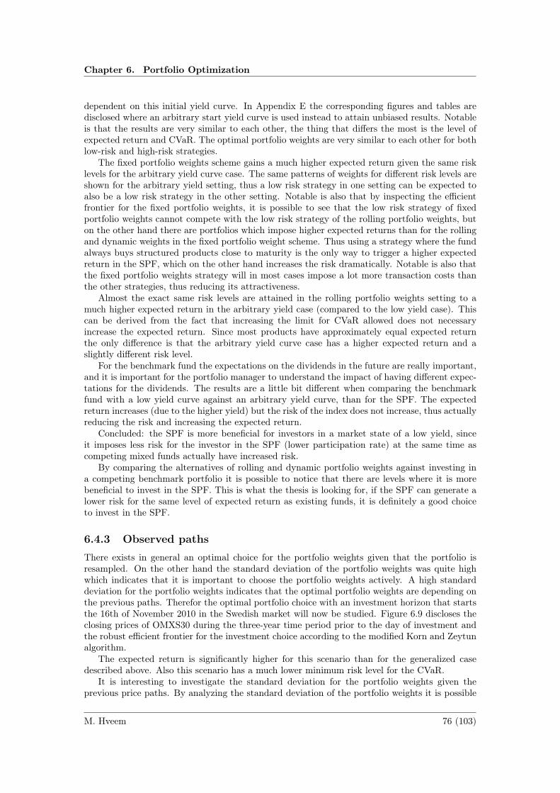
Chapter 6. Portfolio Optimization
dependent on this initial yield curve. In Appendix E the corresponding figures and tables aredisclosed where an arbitrary start yield curve is used instead to attain unbiased results. Notableis that the results are very similar to each other, the thing that differs the most is the level ofexpected return and CVaR. The optimal portfolio weights are very similar to each other for bothlow-risk and high-risk strategies.
The fixed portfolio weights scheme gains a much higher expected return given the same risklevels for the arbitrary yield curve case. The same patterns of weights for different risk levels areshown for the arbitrary yield setting, thus a low risk strategy in one setting can be expected toalso be a low risk strategy in the other setting. Notable is also that by inspecting the efficientfrontier for the fixed portfolio weights, it is possible to see that the low risk strategy of fixedportfolio weights cannot compete with the low risk strategy of the rolling portfolio weights, buton the other hand there are portfolios which impose higher expected returns than for the rollingand dynamic weights in the fixed portfolio weight scheme. Thus using a strategy where the fundalways buys structured products close to maturity is the only way to trigger a higher expectedreturn in the SPF, which on the other hand increases the risk dramatically. Notable is also thatthe fixed portfolio weights strategy will in most cases impose a lot more transaction costs thanthe other strategies, thus reducing its attractiveness.
Almost the exact same risk levels are attained in the rolling portfolio weights setting to amuch higher expected return in the arbitrary yield case (compared to the low yield case). Thiscan be derived from the fact that increasing the limit for CVaR allowed does not necessaryincrease the expected return. Since most products have approximately equal expected returnthe only difference is that the arbitrary yield curve case has a higher expected return and aslightly different risk level.
For the benchmark fund the expectations on the dividends in the future are really important,and it is important for the portfolio manager to understand the impact of having different expec-tations for the dividends. The results are a little bit different when comparing the benchmarkfund with a low yield curve against an arbitrary yield curve, than for the SPF. The expectedreturn increases (due to the higher yield) but the risk of the index does not increase, thus actuallyreducing the risk and increasing the expected return.
Concluded: the SPF is more beneficial for investors in a market state of a low yield, sinceit imposes less risk for the investor in the SPF (lower participation rate) at the same time ascompeting mixed funds actually have increased risk.
By comparing the alternatives of rolling and dynamic portfolio weights against investing ina competing benchmark portfolio it is possible to notice that there are levels where it is morebeneficial to invest in the SPF. This is what the thesis is looking for, if the SPF can generate alower risk for the same level of expected return as existing funds, it is definitely a good choiceto invest in the SPF.
6.4.3 Observed paths
There exists in general an optimal choice for the portfolio weights given that the portfolio isresampled. On the other hand the standard deviation of the portfolio weights was quite highwhich indicates that it is important to choose the portfolio weights actively. A high standarddeviation for the portfolio weights indicates that the optimal portfolio weights are depending onthe previous paths. Therefor the optimal portfolio choice with an investment horizon that startsthe 16th of November 2010 in the Swedish market will now be studied. Figure 6.9 discloses theclosing prices of OMXS30 during the three-year time period prior to the day of investment andthe robust efficient frontier for the investment choice according to the modified Korn and Zeytunalgorithm.
The expected return is significantly higher for this scenario than for the generalized casedescribed above. Also this scenario has a much lower minimum risk level for the CVaR.
It is interesting to investigate the standard deviation for the portfolio weights given theprevious price paths. By analyzing the standard deviation of the portfolio weights it is possible
M. Hveem 76 (103)
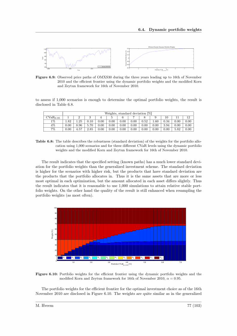
6.4. Dynamic portfolio weights
2008 2009 2010
600
700
800
900
1000
1100
Year
Index
Nasdaq OMXS30
1 2 3 4 5 6 7 826.4
26.6
26.8
27
27.2
27.4
27.6
Efficient Frontier Dynamic Portfolio Weights
Portfolio CVaRα = 0.95
[%]
Expec
ted P
ort
foli
o R
eturn
[%
]
Figure 6.9: Observed price paths of OMXS30 during the three years leading up to 16th of November2010 and the efficient frontier using the dynamic portfolio weights and the modified Kornand Zeytun framework for 16th of November 2010.
to assess if 1,000 scenarios is enough to determine the optimal portfolio weights, the result isdisclosed in Table 6.8.
Weights, standard deviation [%]CVaR0.95 1 2 3 4 5 6 7 8 9 10 11 12
1% 1.82 1.25 0.10 0.00 0.00 0.00 0.00 0.52 1.60 0.34 0.00 0.004% 0.00 8.96 5.70 0.00 0.00 0.00 0.00 0.00 0.00 3.94 0.00 0.007% 0.00 4.57 2.85 0.00 0.00 0.00 0.00 0.00 0.00 0.00 5.82 0.00
Table 6.8: The table describes the robustness (standard deviation) of the weights for the portfolio allo-cation using 1,000 scenarios and for three different CVaR levels using the dynamic portfolioweights and the modified Korn and Zeytun framework for 16th of November 2010.
The result indicates that the specified setting (known paths) has a much lower standard devi-ation for the portfolio weights than the generalized investment scheme. The standard deviationis higher for the scenarios with higher risk, but the products that have standard deviation arethe products that the portfolio allocates in. Thus it is the same assets that are more or lessmost optimal in each optimization, but the amount allocated in each asset differs slightly. Thusthe result indicates that it is reasonable to use 1,000 simulations to attain relative stable port-folio weights. On the other hand the quality of the result is still enhanced when resampling theportfolio weights (as most often).
1.8 2.8 3.8 4.8 5.8 6.8 7.80
10
20
30
40
50
60
70
80
90
100
Wei
ght
[%]
Portfolio CVaRα = 0.95
[%]
w1
w2
w3
w4
w5
w6
w7
w8
w9
w10
w11
w12
Figure 6.10: Portfolio weights for the efficient frontier using the dynamic portfolio weights and themodified Korn and Zeytun framework for 16th of November 2010, α = 0.95.
The portfolio weights for the efficient frontier for the optimal investment choice as of the 16thNovember 2010 are disclosed in Figure 6.10. The weights are quite similar as in the generalized
M. Hveem 77 (103)

Chapter 6. Portfolio Optimization
case, but they differ slightly (adjusted for the particular scenario). Thus it is imperative to adjustthe portfolio optimization depending on the previous observed paths.
6.5 Transaction costs
This section focuses on the dynamic portfolio weights setting and how transaction costs impactthe risk and return levels in comparison to the benchmark fund. The SPF is compared witha benchmark fund, which includes dividends from the index (the most realistic benchmark),for different participation levels as well as for different levels of proportional transaction costs.The transaction costs occur when an asset is bought or sold, all assets have the same level oftransaction costs, for buying as well as selling. Thus rebalancing a portfolio induces transactioncosts, both when the asset is sold and when a new asset is bought. As seen in the previous section;the most desirable setting for the dynamic portfolio weights is to minimize the portfolio’s risk,thus this will be conducted given the constraint of a positive return. Both the setting with alow start yield curve (three years prior to the initial investment horizon) and the setting withan arbitrary start yield curve are investigated. Fixed transaction costs are disregarded to avoidtransforming the problem into a mixed integer linear problem. In Table 6.9 the expected returnand CVaR0.95 for different benchmark funds and SPFs are disclosed.
Table 6.9 indicates that the SPF can compete against different benchmark funds duringdifferent market settings. In the low yield case the SPF provides, in general, lower risk to ahigher expected return than the benchmark fund with an aim of 20% index investments (whenassuming the same transaction costs level). Also the SPF is a lot less risky than the benchmarkfunds at the 30% and 40% levels.
In the arbitrary yield setting: the SPF has higher risk associated with it than the benchmarkfund at 20% level (assuming equal transaction costs for the two funds). On the other hand theSPF has a higher expected return and lower risk than the 30% benchmark fund.
The risk of the SPF increases as the yield increases, since the participation rate increases.Notable is that the risk of the bond part decreases (a bond’s delta is increasing in yield (higheryield, less sensitive to yield changes)), which implies that the benchmark portfolio’s risk decreasesas the yield increases. Thus a fund manager must be aware of these characteristics and how theyimpact the portfolio’s expected return and risk. With a higher yield the bond portfolio gainsa higher return, which explains the higher expected return for both the SPF and benchmarkportfolio in the arbitrary yield setting.
The results indicate that transaction costs is one of the most important concepts for thefund manager to consider in its portfolio. Assume that the proportional transaction costs forstructured products are approximately 3% and for the benchmark portfolio 1%, when studyingthe arbitrary yield case. Thus the SPF’s expected return is 21.83%, has a CVaR0.95 of 7.36%and the benchmark fund which allocates 30% of its assets in the index has an expected returnof 23.08%, a CVaR0.95 of 6.32% (as shown in Table 6.9). Thus the benchmark fund has both ahigher expected return and a lower risk than the SPF, thus it would be an irrational decision toinvest in the SPF.
It is not unreasonable that big funds (or investment banks) have the possibility to invest toas low transaction costs as 0.5% or even 0.25%. Thus the SPF must in the arbitrary yield casehave as low as 1.5% in proportional transaction costs to be more attractive than the benchmarkfund investing 30% of its capital in the index. It is important that the reader takes care andunderstands that these levels are dependent on the data that is used in the modeling, as wellas the underlying assumptions. The same patterns are exhibited for a huge variety of data sets,but the expected returns, CVaR at different levels varies of course. The low yield setting reflectsthe setting of having a yield of approximately 1.5% p.a. in the three-month tenor and 2.3% p.a.for the three-year tenor.
Concluded: the whole idea of a structured products fund is very dependent on the transactioncosts and it is only possible for the fund to compete with other funds, such as mixed funds, if
M. Hveem 78 (103)

6.5. Transaction costs
SPF Dynamic Weights Low yield SPF Dynamic Weights Arbitrary yieldTC [%] Expected Return [%] CVaR0.95 [%] Expected Return [%] CVaR0.95 [%]
0.00 17.69 2.79 27.19 3.990.25 17.26 3.10 26.73 4.290.50 16.82 3.41 26.25 4.591.00 16.00 3.98 25.32 5.161.50 15.21 4.54 24.41 5.732.00 14.44 5.08 23.53 6.282.50 13.70 5.61 22.67 6.823.00 12.97 6.13 21.83 7.36
Benchmark 20% Low yield Benchmark 20% Arbitrary yieldTC Expected Return [%] CVaR0.95 [%] Expected Return [%] CVaR0.95 [%]0.00 15.43 3.25 20.81 0.130.25 15.11 3.39 20.51 0.230.50 14.78 3.70 20.18 0.581.00 14.22 4.18 19.58 1.141.50 13.65 4.70 18.99 1.692.00 13.05 5.09 18.36 2.092.50 12.56 5.56 17.82 2.623.00 11.94 6.10 17.26 3.07
Benchmark 30% Low yield Benchmark 30% Arbitrary yieldTC Expected Return [%] CVaR0.95 [%] Expected Return [%] CVaR0.95 [%]0.00 19.50 8.72 24.37 5.430.25 19.26 8.97 24.04 5.790.50 18.93 9.09 23.75 6.041.00 18.30 9.66 23.08 6.321.50 17.69 10.13 22.59 6.902.00 17.08 10.51 21.97 7.302.50 16.48 10.93 21.28 7.893.00 15.84 11.44 20.68 8.20
Benchmark 40% Low yield Benchmark 40% Arbitrary yieldTC Expected Return [%] CVaR0.95 [%] Expected Return [%] CVaR0.95 [%]0.00 23.88 14.35 28.18 11.460.25 23.56 14.41 27.85 11.640.50 23.20 14.57 27.40 12.001.00 22.58 15.25 26.78 12.411.50 21.87 15.59 26.16 12.752.00 21.32 16.02 25.56 13.172.50 20.64 16.44 24.91 13.613.00 20.07 16.78 24.19 14.15
Table 6.9: The table discloses the expected return and CVaR0.95 for different levels of proportionaltransaction costs for the SPF and benchmark funds over a three-year investment horizonfor both the low yield setting and the arbitrary yield setting.
M. Hveem 79 (103)
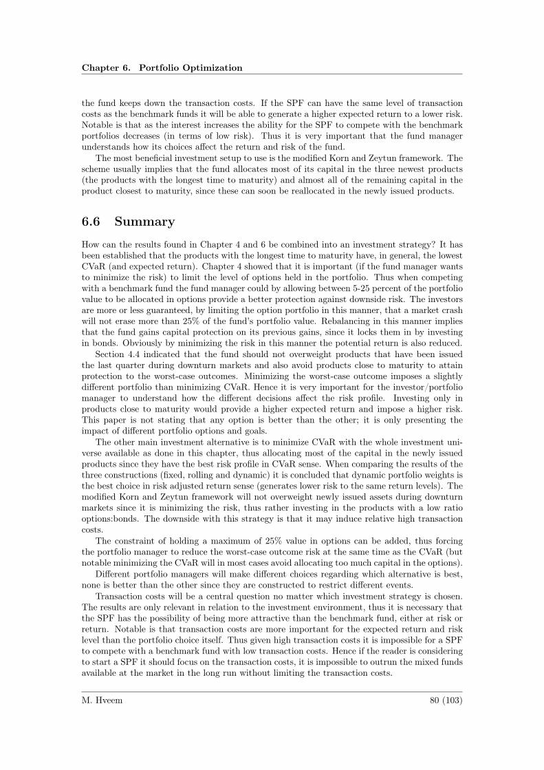
Chapter 6. Portfolio Optimization
the fund keeps down the transaction costs. If the SPF can have the same level of transactioncosts as the benchmark funds it will be able to generate a higher expected return to a lower risk.Notable is that as the interest increases the ability for the SPF to compete with the benchmarkportfolios decreases (in terms of low risk). Thus it is very important that the fund managerunderstands how its choices affect the return and risk of the fund.
The most beneficial investment setup to use is the modified Korn and Zeytun framework. Thescheme usually implies that the fund allocates most of its capital in the three newest products(the products with the longest time to maturity) and almost all of the remaining capital in theproduct closest to maturity, since these can soon be reallocated in the newly issued products.
6.6 Summary
How can the results found in Chapter 4 and 6 be combined into an investment strategy? It hasbeen established that the products with the longest time to maturity have, in general, the lowestCVaR (and expected return). Chapter 4 showed that it is important (if the fund manager wantsto minimize the risk) to limit the level of options held in the portfolio. Thus when competingwith a benchmark fund the fund manager could by allowing between 5-25 percent of the portfoliovalue to be allocated in options provide a better protection against downside risk. The investorsare more or less guaranteed, by limiting the option portfolio in this manner, that a market crashwill not erase more than 25% of the fund’s portfolio value. Rebalancing in this manner impliesthat the fund gains capital protection on its previous gains, since it locks them in by investingin bonds. Obviously by minimizing the risk in this manner the potential return is also reduced.
Section 4.4 indicated that the fund should not overweight products that have been issuedthe last quarter during downturn markets and also avoid products close to maturity to attainprotection to the worst-case outcomes. Minimizing the worst-case outcome imposes a slightlydifferent portfolio than minimizing CVaR. Hence it is very important for the investor/portfoliomanager to understand how the different decisions affect the risk profile. Investing only inproducts close to maturity would provide a higher expected return and impose a higher risk.This paper is not stating that any option is better than the other; it is only presenting theimpact of different portfolio options and goals.
The other main investment alternative is to minimize CVaR with the whole investment uni-verse available as done in this chapter, thus allocating most of the capital in the newly issuedproducts since they have the best risk profile in CVaR sense. When comparing the results of thethree constructions (fixed, rolling and dynamic) it is concluded that dynamic portfolio weights isthe best choice in risk adjusted return sense (generates lower risk to the same return levels). Themodified Korn and Zeytun framework will not overweight newly issued assets during downturnmarkets since it is minimizing the risk, thus rather investing in the products with a low ratiooptions:bonds. The downside with this strategy is that it may induce relative high transactioncosts.
The constraint of holding a maximum of 25% value in options can be added, thus forcingthe portfolio manager to reduce the worst-case outcome risk at the same time as the CVaR (butnotable minimizing the CVaR will in most cases avoid allocating too much capital in the options).
Different portfolio managers will make different choices regarding which alternative is best,none is better than the other since they are constructed to restrict different events.
Transaction costs will be a central question no matter which investment strategy is chosen.The results are only relevant in relation to the investment environment, thus it is necessary thatthe SPF has the possibility of being more attractive than the benchmark fund, either at risk orreturn. Notable is that transaction costs are more important for the expected return and risklevel than the portfolio choice itself. Thus given high transaction costs it is impossible for a SPFto compete with a benchmark fund with low transaction costs. Hence if the reader is consideringto start a SPF it should focus on the transaction costs, it is impossible to outrun the mixed fundsavailable at the market in the long run without limiting the transaction costs.
M. Hveem 80 (103)

6.7. Backtesting
6.7 Backtesting
This section investigates how the modified Korn and Zeytun algorithm would have performedhistorically. The model is backtested from the beginning of 2002 to the middle of 2010 (datafor OMXS30 total return is only available since 2002 from Bloomberg). In each time step thesimulation is based on the last four year’s data (log returns), to capture approximately a marketcycle. Proportional transaction costs at the levels 0%, 1%, 2% and 3% are considered. TheCVaR is minimized given the constraint of a positive return. Notable is that the scheme is onlyrebalancing matured capital, to avoid as much unnecessary transaction costs as possible. Theresults are compared with the benchmark fund described earlier (with 30% market participation),which is based on the total return version of OMXS30, and with the actual OMXS30 total returnversion. Figure 6.11 shows that the SPF had the desired characteristics during the financialturmoil during 2002 and during 2008-2009, imposing a high level of capital protection. Also theSPF did not actually yield any return during the latter part of 2009 and 2010, rather negativereturn. This is due to that the portfolio is rebalanced quite significantly during the last quarters(imposing negative returns due to transaction costs) and the volatility drops significantly, whichimplies that the value of the options decreases. The interest rate movements also impact thereturn during these quarters negative, the increase in the yield results in lower bond prices.
2003 2004 2005 2006 2007 2008 2009 2010
60
80
100
120
140
160
Year
[%]
Nasdaq OMXS30 Total Return
NAV Fund
SPF Benchmark
(a) TC = 0%, SPF total return 51.73%.
2003 2004 2005 2006 2007 2008 2009 2010
60
80
100
120
140
160
Year
[%]
Nasdaq OMXS30 Total Return
NAV Fund
SPF Benchmark
(b) TC = 1%, SPF total return 43.35%.
2003 2004 2005 2006 2007 2008 2009 2010
60
80
100
120
140
160
Year
[%]
Nasdaq OMXS30 Total Return
NAV Fund
SPF Benchmark
(c) TC = 2%, SPF total return 36.73%.
2003 2004 2005 2006 2007 2008 2009 2010
60
80
100
120
140
160
Year
[%]
Nasdaq OMXS30 Total Return
NAV Fund
SPF Benchmark
(d) TC = 3%, SPF total return 29.25%.
Figure 6.11: Backtesting results for the dynamic portfolio weights SPF against a benchmark mixedfund with 30% participation rate and OMXS30.
The transaction costs impact the return significantly (notable is that the benchmark fundsuffers in approximately the same extent). The problem with investing using a structured prod-ucts fund is that the structured products mature and the capital must be reinvested in newproducts, imposing new transaction costs. Thus if the fund instead invests in products that havea longer time to maturity it is possible to both reduce the risk (since products with a longer timeto maturity have lower risk) and the transaction costs.
A backtest is also conducted for the fixed portfolio weights strategy using the algorithm fromSection 6.1 and in Figure 6.3, which takes in count the transaction costs, thus allocating mostlyin the newly issued products, the result is disclosed in Figure 6.12. This strategy generates ahigher return than the dynamic portfolio weights strategy during the time period, which is moredue to a coincidence than an optimal portfolio choice, since this is just one observation. The fixedportfolio weights setting generates higher transaction costs than the dynamic portfolio weightssetting.
It is really important to not rebalance the whole portfolio every quarter, instead the fundshould mainly rebalance capital that has matured, in a setting with high transaction costs.Rebalancing the whole portfolio every quarter would in the dynamic portfolio weights setting,
M. Hveem 81 (103)

Chapter 6. Portfolio Optimization
2003 2004 2005 2006 2007 2008 2009 2010
60
80
100
120
140
160
Year
[%]
Nasdaq OMXS30 Total Return
NAV Fund
SPF Benchmark
(a) TC = 0%, SPF total return 63.64%.
2003 2004 2005 2006 2007 2008 2009 2010
60
80
100
120
140
160
Year
[%]
Nasdaq OMXS30 Total Return
NAV Fund
SPF Benchmark
(b) TC = 1%, SPF total return 45.86%.
2003 2004 2005 2006 2007 2008 2009 2010
60
80
100
120
140
160
Year
[%]
Nasdaq OMXS30 Total Return
NAV Fund
SPF Benchmark
(c) TC = 2%, SPF total return 33.81%.
2003 2004 2005 2006 2007 2008 2009 2010
60
80
100
120
140
160
Year
[%]
Nasdaq OMXS30 Total Return
NAV Fund
SPF Benchmark
(d) TC = 3%, SPF total return 30.60%.
Figure 6.12: Backtesting results for the fixed portfolio weights SPF including proportional transactioncosts against a benchmark mixed fund with 30% participation rate and OMXS30.
with 3% in transaction costs, yield 15% in return instead of approximately 29%. Thus theportfolio manager should assume a type of buy and hold strategy and mainly reallocate maturedcapital. If the fund assumes a buy and hold strategy the portfolio manager should be awareof that it still needs to rebalance the whole portfolio sometimes, e.g. when the option portfoliovalue exceeds its allowed boundary.
Thus it is recommended that, in a setting of high transaction costs, the portfolio manageruses the modified Korn and Zeytun framework to initially allocate its capital, and to reallocatethe matured capital. The importance of using a more active portfolio strategy is higher whenthe possibility of diversifying in several structured products with different underlying exists.
M. Hveem 82 (103)

CHAPTER 7
Conclusions
The thesis has studied the concept of a structured products fund (SPF) and how it should beconstructed to be competitive in risk sense. The study shows that the concept should not bedisregarded and that it is possible to construct a SPF that is competitive.
Transaction costs affect the expected return and risk level for the SPF in a high extent. Thusthe study indicates that the most important factor for a portfolio manager to consider is thetransaction costs. A SPF with high transaction costs will not have the possibility of beating thecompeting mixed funds at either risk or return. Thus the fund needs low transaction costs (inlevel with the competing funds) in order to not increase the risk and decrease the return in a toohigh extent.
The study focuses a lot on the issue of capital guarantee since it is desirable that the SPFhas the same characteristics as a capital guaranteed product. The study indicates that it is notpossible to attain a portfolio based on structured products that is capital guaranteed. The thesisinstead studies the concept of alternative capital protection and finds that a fund can be capitalprotected at a certain level for a given risk measure, the thesis uses the risk measure CVaR.Thus a fund that has a CVaR0.90 less than for example 0% can claim that the portfolio is capitalprotected on a 100% level with a confidence level of 90%. CVaR is used as a risk measure sinceit captures both skewness and kurtosis and is adequate to use in scenario based optimization. Itis also common to describe a fund’s risk characteristics via CVaR, thus making it an adequaterisk measure to benchmark through.
The thesis finds that a portfolio manager has mainly two investment schemes to allocatethe portfolio with, to minimize the downside risk, thus attaining as much capital protection aspossible. The first investment scheme is a type of rolling investment scheme where the portfoliomanager invests broadly in almost all the available products (preferably equal weights). Thefund should sell of the products when they are close to maturity (a quarter or two left), sincethese assets exhibit a lot of risk especially if they are in the money. The capital that is gainedwhen assets are sold should be reinvested in the newly issued products since they have in generalthe lowest risk associated with them. On the other hand as the index starts to decrease (duringbear markets) the portfolio should underweight newly issued products (products with the longesttime to maturity) since they are risky products in downturn markets. This scheme is used toboth restrict the risk and the induced transaction costs. The benefit with this scheme is thatit is easy to implement and that it serves as a reasonable investment choice during most timeperiods. On the other hand the scheme can induce a high-risk portfolio during unwanted marketstates, since it does not adjust to changes in the market. Thus it is impossible to control theexpected return of the investment as well as the risk level. Hence the thesis instead proposes amore sophisticated allocation algorithm, which is referred to as the modified Korn and Zeytunframework.
The modified Korn and Zeytun framework is used to minimize the risk (CVaR) given theconstraint of the expected return. This framework is very beneficial and creates low risk portfolioswith high expected return. The framework that is presented in detail in Section 6.4 shows thatit is possible to generate portfolios that have a higher expected return than competing funds toa lower risk, given that the transaction costs are low. The study is conducted with both low
83
Chapter 7. Conclusions
yield and arbitrary yield start trajectories. The results show that a SPF is most beneficial duringtimes of low yield since the risk of the SPF increases a lot as the yield goes up.
The results indicate that a SPF can be a superb investment vehicle for investors searchingfor low risk alternatives with a limited downside. They also show that it is imperative that aportfolio manager understands how the portfolio allocation affects the characteristics of the fund,since it is a rather complex issue.
It is strongly recommended to use the modified Korn and Zeytun framework to allocate theportfolio with, for a SPF, since it generates well-balanced portfolios in risk and return sense.Allocating according to the modified Korn and Zeytun framework will in most cases lead toallocating in the best available portfolio (given the constraints) in every time step since it canbe used for specific paths (adjust for the current market data).
The thesis finds that it is important, no matter which scheme is used, that the portfolio isnot allowed to hold more than a certain degree of value attained in options (a limit), to avoiddownside risk for its investors. A recommended level is that the SPF is allowed to allocate amaximum of 25% of its capital in options (within the structured products) with a target level of15%. The portfolio should be rebalanced if this limit is exceeded, hence reducing the downsiderisk.
The thesis studies ELNs with a time to maturity of three years and the results can begeneralized to products with a longer time to maturity at issuance (newly issued products, lessrisk). The thing that differs for a capital guaranteed ELN with a time to maturity of three yearsat issuance and one with a longer time to maturity (or shorter) is the ratio options:bonds. Thusa newly issued ELN with five years to maturity has a higher risk than a newly issued ELN withthree years to maturity since it has a higher proportion options. Thus it is very important to usethe boundaries of allowed proportion options:bonds especially when combining different types ofELNs. The big advantage by using the modified Korn and Zeytun framework is that it adjustsfor these discrepancies and that the portfolio manager does not need to modify the allocationmodel if it modifies its investment universe.
Thus the main result is: yes it is possible to construct a fund based on structured productsthat is competitive and exhibits a type of capital protection (i.e. in CVaR sense). Only oneunderlying for the ELNs has been used and the results can be generalized without serious lossof generality to the multi-dimensional case. A Black-Litterman approach to the optimizationproblem is left for future studies where it, in combination with the multi-underlying case, canprovide superior return due to subjective views on the market.
M. Hveem 84 (103)

Bibliography
[1] Aas, K. (2006). The Generalised Hyperbolic Skew Student’s t-distribution. Journal of Fi-nancial Econometrics, 4 (2), 275-309.
[2] Abdi, H., & Williams, L. J. (2010). Principal Component Analysis. Wiley InterdisciplinaryReviews: Computational Statistics, 2, 1-47.
[3] Acerbi, C. (2002). Spectral measures of risk: A coherent representation of subjective riskaversion. Journal of Banking & Finance, 26 (7), 1505-1518.
[4] Alexander, S., Coleman, T.F., & Li, Y. (2006). Minimizing CVaR and VaR for a portfolioof derivatives. Journal of Banking & Finance, 30 (2), 583-605.
[5] Bank For International Settlements. (2006). Basel II: International Convergence of CapitalMeasurement and Capital Standards: A Revised Framework. Basel: BIS
[6] Barber, J. R., & Copper, M. L. (2010). Principal component analysis of yield curve move-ments. Journal of Economics and Finance, 1-16, doi:10.1007/s12197-010-9142-y.
[7] Björk, T. (2009). Arbitrage Theory in Continuous Time (3rd ed.). Oxford: Oxford Finance.
[8] Black, F., & Litterman, R. (1992). Global Portfolio Optimization. Financial Analysts Jour-nal, 48 (5), 28-43.
[9] Black, F., & Scholes, M. (1973). The Pricing of Options and Corporate Liabilities. Journalof Political Economy, 81 (3), 637-654.
[10] Brooks, C., & Persand, G. (2000). Value at Risk and Market Crashes. Discussion Paper inFinance 2000-01. University of Reading.
[11] Browning, E., S. (2007, October 15). Exorcising Ghosts of Octobers Past, Wall Street Jour-nal, p. C1.
[12] Chuan, T. (2008, August, 5). Capital Protected is not Capital Guaranteed. Financial Plan-ning Central:http://www.ifa-sg.com/capital-protected-is-not-capital-guaranteed/
[13] Deng, G., Li, G., Liu, S., Mallett, J., & McCann, C. (2009). Structured Products In theAftermath of Lehman Brothers. Working Papers Securities Litigation & Consulting Group.
[14] Fisher, A. (1999). Multivariate Stock Returns Around Extreme Events: A Reassessment ofEconomic Fundamentals and the 1987 Market Crash. NYU Working Paper, No. FIN-99-071.
[15] Frazzini, A. (2006). The Disposition Effect and Underreaction to News. The Journal ofFinance, 61 (4), 2017-2046.
[16] Glot, P. (2005). Relationship Between Implied Volatility Indexes and Stock Index Returns.The Journal of Portfolio Management, 31 (3), 92-100.
[17] Grinold, R., C. (1999). Mean-Variance and Scenario-Based Approaches to Portfolio Selec-tion. Journal of Portfolio Management, 25 (2), 10-22.
85

Bibliography
[18] Hagan, P. S., Kumar, D., Lesniewski, A. S., & Woodward, D. E. (2002). Managing SmileRisk. Wilmott Magazine September 2002, 84-108.
[19] Hansen, P., & Lärfars, M. (2010). Evaluating Long-Term Performance of Structured Prod-ucts. Stockholm: Kungliga Tekniska Högskolan.
[20] Heston, S. L. (1993). A Closed-Form Solution for Options with Stochastic Volatility withApplications to Bond and Currency Options. The Review of Financial Studies, 6 (2), 327-343.
[21] HSBC. (2010, September 14). Structured Product Glossary. HSBC:http://www.hsbcnet.com/treasury/structured-products/wms-global/struc_prod_glossary.html
[22] Hull, J.C. (2002). Options, Futures, and Other, Derivatives (5th ed.). New Jersey: PrenticeHall.
[23] Hult, H., & Lindskog, F. (2009). Lecture notes in Risk management. Stockholm: RoyalInstitute of Technology.
[24] Hult, H., Lindskog, F., Hammarlid, O., & Rehn, C.-J. (2010). Risk and portfolio analysis:principles and methods, Part I. Stockholm: Royal Institute of Technology.
[25] Johansson, T., & Lingnardz, H. (2010). Evaluation of Equity-Linked Notes - an EmpiricalStudy of SEB Equity-Linked Notes. Lund: Lund University.
[26] Kahneman, D., & Tversky, A. (1979). Prospect Theory: An Analysis of Decision under Risk.Econometrica, 47 (2), 263-291.
[27] Korn, R., & Zeytun, S. (2009). Solving optimal investment problems with structured prod-ucts under CVaR constraints. Optimization, 58 (3), 291-304.
[28] Krokhmal, P., Palmquist, J., & Uryasev, S. (2002). Portfolio optimization with conditionalvalue-at-risk objective and constraints. Journal of Risk, 4 (2), 11-27.
[29] Litterman, R., & Scheinkman, J. (1991). Common Factors Affecting Bond Returns. TheJournal of Fixed Income, 1 (1), 54-61.
[30] Markowitz, H. (1952). Portfolio selection. Journal of Finance, 7 (1), 77-91.
[31] Martellini, L., Simsek, K., & Goltz, K. (2005). Structured forms of investment strategiesin institutional investors portfolios. Technical report, EDHEC Risk and Asset ManagementResearch Centre.
[32] My News Desk. (2010, January 29). Swedbank störst på indexobligationer. My News Desk:http://www.mynewsdesk.com/se/pressroom/swedbank/pressrelease/view/swedbank-stoerst-paa-indexobligationer-366818
[33] Rockafellar, R., T., & Uryasev, P. (2001). Conditional Value-at-Risk for General Loss Dis-tributions. ISE Dept. Working Paper No. 2001-5.
[34] Scherer, B. (2004) Portfolio Construction and Risk Budgeting (2nd ed.). London: RiskBooks.
[35] Shefrin, H. (2002). Beyond Greed and Fear (2nd ed.). Oxford: Oxford University Press.
[36] Soto, G. (2004) Using Principal Component Analysis to Explain Term Structure Movements:Performance and Stability. Available online at: http://ssrn.com/abstract=985404.
M. Hveem 86 (103)

Bibliography
[37] UBG AG. (2010, October, 12). Banking terms. UBS AG:http://www.ubs.com/1/e/gcc/bankingterms.html.
[38] Uryasev, P. (2000). Conditional Value-at-Risk: Optimization Algorithms and Applications.Financial Engineering News, 14, 1-5.
[39] Wasserfallen, W., & Schenk, C. (1996). Portfolio Insurance for the Small Investor in Switzer-land, The Journal of Derivatives, 3 (3), 37-43.
M. Hveem 87 (103)


Appendices
89


APPENDIX ANaive fund constructions - Additional scenarios
Naive fund construction 1
0 5 10 15 20 250
50
100
150
200
250
X: 24Y: 92.13
Quarter
$
Price Underlying
NAV Fund
Start of investment
(a) Scenario 3, −7.87%.
0 5 10 15 20 250
20
40
60
80
100
120
X: 24Y: 100
Quarter
$Price Underlying
NAV FundStart of investment
(b) Scenario 4, 0%.
0 5 10 15 20 250
20
40
60
80
100
120
X: 24Y: 92.28
Quarter
[%]
Volatility
NAV FundStart of investment
(c) Scenario 5, −7.72%.
0 5 10 15 20 250
20
40
60
80
100
120
X: 24
Y: 89.76
Quarter
[%]
Interest Rate
NAV FundStart of investment
(d) Scenario 6, −10.24%.
Figure A.1: Scenarios 3-6, return between Q12-Q24.
91


APPENDIX BOption portfolios - Additional portfolios
w9 =(
1 0 0 0 0 0 0 0 0 0 0 0)T
w10 =(
0 1 0 0 0 0 0 0 0 0 0 0)T
w11 =(
0 0 0 0 0 0 0 0 0 0 1 0)T
w12 =(
0 0 110
110
110
110
110
110
110
110
110
110
)Tw13 =
(0 0 0 0 1
818
18
18
18
18
18
18
)Tw14 =
(14
14
14
14 0 0 0 0 0 0 0 0
)Tw15 =
(0 0 0 0 1
414
14
14 0 0 0 0
)Tw16 =
(0 0 0 0 0 0 0 0 1
414
14
14
)Tw17 =
(0 0 0 0 0 0 0 0 1
10310
310
310
)Tw18 =
(18
18
18
18
18
18
18
18 0 0 0 0
)Tw19 =
(18
18
18
18 0 0 0 0 1
818
18
18
)T
−1 −0.8 −0.6 −0.4 −0.2 0 0.2 0.40
200
400
600
800
1000
1200
Option portfolio average monthly returns (36 months periods)
Average return per month
Ou
tco
mes
(a) Portfolio 9, −100%.
−0.5 −0.4 −0.3 −0.2 −0.1 0 0.1 0.20
500
1000
1500
2000
2500
Option portfolio average monthly returns (36 months periods)
Average return per month
Ou
tco
mes
(b) Portfolio 10, −47.37%.
−0.2 −0.15 −0.1 −0.05 0 0.05 0.1 0.150
50
100
150
200
250
300
Option portfolio average monthly returns (36 months periods)
Average return per month
Ou
tco
mes
(c) Portfolio 11, −19.02%.
Figure B.1: Histograms over the outcomes for option portfolios 9-11, the worst-case average 36 monthreturn is given in the caption.
93

Appendix B. Option portfolios - Additional portfolios
−0.25 −0.2 −0.15 −0.1 −0.05 0 0.05 0.1 0.150
20
40
60
80
100
120
140
160
180
Option portfolio average monthly returns (36 months periods)
Average return per month
Ou
tco
mes
(a) Portfolio 12, −20.55%.
−0.25 −0.2 −0.15 −0.1 −0.05 0 0.05 0.1 0.150
50
100
150
200
250
Option portfolio average monthly returns (36 months periods)
Average return per month
Ou
tco
mes
(b) Portfolio 13, −20.93%.
−0.4 −0.3 −0.2 −0.1 0 0.1 0.2 0.30
100
200
300
400
500
600
Option portfolio average monthly returns (36 months periods)
Average return per month
Outc
om
es
(c) Portfolio 14, −39.94%.
−0.3 −0.25 −0.2 −0.15 −0.1 −0.05 0 0.05 0.1 0.150
50
100
150
200
250
Option portfolio average monthly returns (36 months periods)
Average return per month
Outc
om
es
(d) Portfolio 15, −26.46%.
−0.2 −0.15 −0.1 −0.05 0 0.05 0.1 0.150
50
100
150
200
250
Option portfolio average monthly returns (36 months periods)
Average return per month
Outc
om
es
(e) Portfolio 16, −20.44%.
−0.25 −0.2 −0.15 −0.1 −0.05 0 0.05 0.1 0.150
50
100
150
200
250
Option portfolio average monthly returns (36 months periods)
Average return per month
Ou
tco
mes
(f) Portfolio 17, −20.74%.
−0.25 −0.2 −0.15 −0.1 −0.05 0 0.05 0.1 0.150
20
40
60
80
100
120
140
160
Option portfolio average monthly returns (36 months periods)
Average return per month
Ou
tco
mes
(g) Portfolio 18, −24.04%.
−0.25 −0.2 −0.15 −0.1 −0.05 0 0.05 0.1 0.150
20
40
60
80
100
120
140
160
180
Option portfolio average monthly returns (36 months periods)
Average return per month
Ou
tco
mes
(h) Portfolio 19, −24.47%.
Figure B.2: Histograms over the outcomes for option portfolios 12-19, the worst-case average 36 monthreturn is given in the caption.
M. Hveem 94 (103)
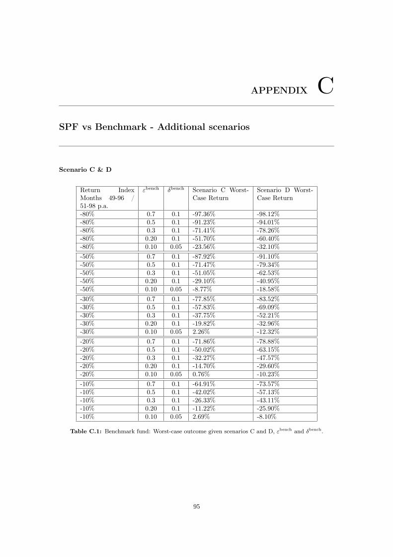
APPENDIX CSPF vs Benchmark - Additional scenarios
Scenario C & D
Return IndexMonths 49-96 /51-98 p.a.
εbench δbench Scenario C Worst-Case Return
Scenario D Worst-Case Return
-80% 0.7 0.1 -97.36% -98.12%-80% 0.5 0.1 -91.23% -94.01%-80% 0.3 0.1 -71.41% -78.26%-80% 0.20 0.1 -51.70% -60.40%-80% 0.10 0.05 -23.56% -32.10%-50% 0.7 0.1 -87.92% -91.10%-50% 0.5 0.1 -71.47% -79.34%-50% 0.3 0.1 -51.05% -62.53%-50% 0.20 0.1 -29.10% -40.95%-50% 0.10 0.05 -8.77% -18.58%-30% 0.7 0.1 -77.85% -83.52%-30% 0.5 0.1 -57.83% -69.09%-30% 0.3 0.1 -37.75% -52.21%-30% 0.20 0.1 -19.82% -32.96%-30% 0.10 0.05 2.26% -12.32%-20% 0.7 0.1 -71.86% -78.88%-20% 0.5 0.1 -50.02% -63.15%-20% 0.3 0.1 -32.27% -47.57%-20% 0.20 0.1 -14.70% -29.60%-20% 0.10 0.05 0.76% -10.23%-10% 0.7 0.1 -64.91% -73.57%-10% 0.5 0.1 -42.02% -57.13%-10% 0.3 0.1 -26.33% -43.11%-10% 0.20 0.1 -11.22% -25.90%-10% 0.10 0.05 2.69% -8.10%
Table C.1: Benchmark fund: Worst-case outcome given scenarios C and D, εbench and δbench.
95

Appendix C. SPF vs Benchmark - Additional scenarios
Scenario C Scenario DMonths 0-48, return 30% p.a. Months 0-48, return 30% p.a.Months 48-49, return -80% p.m. Months 48-50, return 50% p.a.Months 49-96, return -X% p.a. Months 50-51, return -80% p.m.Months 96-144, return 30% p.a. Months 51-98, return -X% p.a.
Months 98-144, return 30% p.a.
Return IndexMonths 49-96 /51-98 p.a.
εSPF δSPF Scenario C Worst-Case Return
Scenario D Worst-Case Return
-80% 1 1 -20.35% -61.49%-80% 0.3 0.1 -20.35% -61.49%-80% 0.25 0.1 -11.25% -51.12%-80% 0.20 0.1 -10.42% -50.03%-80% 0.15 0.1 1.32% -30.87%-80% 0.10 0.05 3.79% -25.69%-50% 1 1 -20.65% -62.31%-50% 0.3 0.1 -20.65% -62.31%-50% 0.25 0.1 -11.58% -52.17%-50% 0.20 0.1 -10.76% -51.10%-50% 0.15 0.1 0.94% -32.25%-50% 0.10 0.05 3.41% -27.27%-30% 1 1 -24.26% -63.95%-30% 0.3 0.1 -24.26% -63.95%-30% 0.25 0.1 -15.61% -54.24%-30% 0.20 0.1 -14.82% -53.22%-30% 0.15 0.1 -3.65% -35.28%-30% 0.10 0.05 -1.30% -30.43%-20% 1 1 -25.671% -64.62%-20% 0.3 0.1 -25.67% -64.62%-20% 0.25 0.1 -17.18% -55.09%-20% 0.20 0.1 -16.41% -54.09%-20% 0.15 0.1 -5.45% -36.48%-20% 0.10 0.05 -3.14% -31.72%-10% 1 1 -26.26% -64.91%-10% 0.3 0.1 -26.26% -64.91%-10% 0.25 0.1 -17.84% -55.46%-10% 0.20 0.1 -17.07% -54.47%-10% 0.15 0.1 -6.20% -37.00%-10% 0.10 0.05 -3.91% -32.28%
Table C.2: SPF 1: Worst-case outcomes for the SPF 1 Portfolio 7 given the scenarios C and D, εSPF
and δSPF.
M. Hveem 96 (103)

Portfolio 3, Scenario A & B
Return IndexMonths 48-96 /50-98 p.a.
εSPF δSPF Scenario A Worst-Case Return
Scenario B Worst-Case Return
-80% 1 1 -26.11% -57.88%-80% 0.25 0.1 -26.11% -40.90%-80% 0.20 0.1 -19.68% -35.51%-80% 0.15 0.1 -15.98% -26.94%-80% 0.15 0.05 -14.77% -29.43%-80% 0.10 0.05 -13.02% -20.77%-50% 1 1 -24.87% -49.59%-50% 0.25 0.1 -24.87% -31.78%-50% 0.20 0.1 -18.96% -27.15%-50% 0.15 0.1 -16.01% -19.28%-50% 0.15 0.05 -16.69% -23.33%-50% 0.10 0.05 -12.71% -14.78%-30% 1 1 -20.46% -37.45%-30% 0.25 0.1 -20.46% -22.40%-30% 0.20 0.1 -15.21% -16.62%-30% 0.15 0.1 -12.92% -9.19%-30% 0.15 0.05 -13.19% -13.63%-30% 0.10 0.05 -8.82% -12.84%-20% 1 1 -16.53% -26.71%-20% 0.25 0.1 -16.53% -12.91%-20% 0.20 0.1 -11.56% -8.31%-20% 0.15 0.1 -8.71% -1.35%-20% 0.15 0.05 -9.36% -5.38%-20% 0.10 0.05 -5.12% -0.79%-10% 1 1 -9.92% -13.72%-10% 0.25 0.1 -9.92% -3.5%-10% 0.20 0.1 -5.94% -1.28%-10% 0.15 0.1 -0.53% 5.44%-10% 0.15 0.05 -4.49% 0.00%-10% 0.10 0.05 0.00% 3.35%
Table C.3: SPF 1: Worst-case outcomes for the SPF 1 Portfolio 3 given scenarios A and B, εSPF andδSPF.
M. Hveem 97 (103)

Appendix C. SPF vs Benchmark - Additional scenarios
Stress testing
µ = −30% p.a. for underlying instead of 0% p.a. as in Section 4.4.7
−0.4 −0.2 0 0.2 0.4 0.6 0.8 10
500
1000
1500
2000
2500
3000
3500Histogram over the SPF:s 36 month (overlapping) returns
Return
Outc
om
es
(a) SPF 1: εSPF = 0.15, δSPF =0.1, min: −20.59%, mean:8.01%, max: 63.24%.
−0.4 −0.3 −0.2 −0.1 0 0.1 0.2 0.3 0.4 0.50
500
1000
1500
2000
2500Histogram over the Benchmark funds 36 month (overlapping) returns
Return
Outc
om
es
(b) Benchmark: εbench = 0.3,δbench = 0.1, min: −37.83%,mean: −7.70%, max: 45.03%.
−1 −0.5 0 0.5 1 1.50
500
1000
1500
2000
2500
3000
3500
4000Histogram over the Underlying 36 month (overlapping) returns
Return
Outc
om
es
(c) Underlying: min: −92.60%,mean: −56.87%, max: 129.82%.
Figure C.1: Histograms over 36 months returns for the competing funds and the modified stress test
Backtesting
1996 1998 2000 2002 2004 2006 2008 2010 2012100
150
200
250
300
350
400
Year
$
Nasdaq OMXS30
NAV Fund
NAV Benchmark
(a) εSPF = 0.10, δSPF = 0.05.
1996 1998 2000 2002 2004 2006 2008 2010 2012100
150
200
250
300
350
400
Year
$
Nasdaq OMXS30
NAV Fund
NAV Benchmark
(b) εSPF = 0.15, δSPF = 0.1.
1996 1998 2000 2002 2004 2006 2008 2010 2012100
150
200
250
300
350
400
Year
$
Nasdaq OMXS30
NAV Fund
NAV Benchmark
(c) εSPF = 0.2, δSPF = 0.1.
1996 1998 2000 2002 2004 2006 2008 2010 2012100
150
200
250
300
350
400
Year
$
Nasdaq OMXS30
NAV Fund
NAV Benchmark
(d) εSPF = 0.25, δSPF = 0.1.
Figure C.2: Backtest results: OMXS30 vs SPF 1 (Portfolio 4) and Benchmark..
M. Hveem 98 (103)

APPENDIX DCorrelations between the market index and the yield curve
Correlation matrix between OMXS30 and SEK yield curve, daily log returns (Jan 1996 - Nov 2010).Index 1M 2M 3M 6M 9M 1Y 2Y 3Y
Index 1.0000 -0.0080 -0.0023 -0.0117 0.0012 0.0070 0.0193 0.1900 0.18911M -0.0080 1.0000 0.8970 0.8559 0.7678 0.7081 0.6855 0.3166 0.23822M -0.0023 0.8970 1.0000 0.9149 0.8422 0.7850 0.7628 0.3610 0.28023M -0.0117 0.8559 0.9149 1.0000 0.8947 0.8429 0.8229 0.3914 0.30706M 0.0012 0.7678 0.8422 0.8947 1.0000 0.9362 0.9214 0.4487 0.36579M 0.0070 0.7081 0.7850 0.8429 0.9362 1.0000 0.9610 0.4783 0.41001Y 0.0193 0.6855 0.7628 0.8229 0.9214 0.9610 1.0000 0.4981 0.43172Y 0.1900 0.3166 0.3610 0.3914 0.4487 0.4783 0.4981 1.0000 0.89163Y 0.1891 0.2382 0.2802 0.3070 0.3657 0.4100 0.4317 0.8916 1.0000
Correlation matrix between OMXS30 and SEK yield curve, weekly log returns (Jan 1996 - Nov 2010).Index 1M 2M 3M 6M 9M 1Y 2Y 3Y
Index 1.0000 -0.0504 -0.0484 -0.0458 -0.0211 -0.0120 -0.0000 0.1741 0.18991M -0.0504 1.0000 0.9431 0.8971 0.8016 0.7497 0.7226 0.3765 0.26662M -0.0484 0.9431 1.0000 0.9578 0.8897 0.8471 0.8191 0.4488 0.33783M -0.0458 0.8971 0.9578 1.0000 0.9345 0.8965 0.8693 0.4975 0.39156M -0.0211 0.8016 0.8897 0.9345 1.0000 0.9711 0.9513 0.5965 0.49939M -0.0120 0.7497 0.8471 0.8965 0.9711 1.0000 0.9864 0.6438 0.56461Y -0.0000 0.7226 0.8191 0.8693 0.9513 0.9864 1.0000 0.6684 0.59722Y 0.1741 0.3765 0.4488 0.4975 0.5965 0.6438 0.6684 1.0000 0.94123Y 0.1899 0.2666 0.3378 0.3915 0.4993 0.5646 0.5972 0.9412 1.0000
Correlation matrix between OMXS30 and SEK yield curve, monthly log returns (Jan 1996 - Nov 2010).Index 1M 2M 3M 6M 9M 1Y 2Y 3Y
Index 1.0000 -0.1041 -0.1328 -0.1320 -0.1029 -0.0935 -0.0757 0.1121 0.12331M -0.1041 1.0000 0.9608 0.9258 0.8415 0.7791 0.7473 0.5317 0.38372M -0.1328 0.9608 1.0000 0.9777 0.9166 0.8634 0.8325 0.5900 0.44103M -0.1320 0.9258 0.9777 1.0000 0.9553 0.9134 0.8849 0.6419 0.49126M -0.1029 0.8415 0.9166 0.9553 1.0000 0.9800 0.9626 0.7399 0.59659M -0.0935 0.7791 0.8634 0.9134 0.9800 1.0000 0.9932 0.7940 0.66771Y -0.0757 0.7473 0.8325 0.8849 0.9626 0.9932 1.0000 0.8223 0.70482Y 0.1121 0.5317 0.5900 0.6419 0.7399 0.7940 0.8223 1.0000 0.95633Y 0.1233 0.3837 0.4410 0.4912 0.5965 0.6677 0.7048 0.9563 1.0000
99

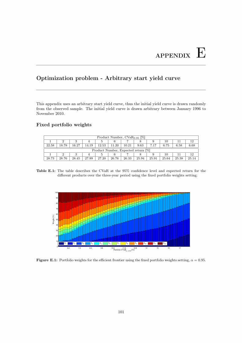
APPENDIX EOptimization problem - Arbitrary start yield curve
This appendix uses an arbitrary start yield curve, thus the initial yield curve is drawn randomlyfrom the observed sample. The initial yield curve is drawn arbitrary between January 1996 toNovember 2010.
Fixed portfolio weights
Product Number, CVaR0.95 [%]1 2 3 4 5 6 7 8 9 10 11 12
22.58 18.78 16.27 14.19 12.53 11.20 10.21 9.63 7.17 6.75 6.58 6.68Product Number, Expected return [%]
1 2 3 4 5 6 7 8 9 10 11 1228.73 28.76 28.45 27.99 27.20 26.76 26.33 25.94 25.91 25.64 25.38 25.14
Table E.1: The table describes the CVaR at the 95% confidence level and expected return for thedifferent products over the three-year period using the fixed portfolio weights setting.
6.2 7.4 8.4 9.6 10.6 11.8 12.8 14 15 16 170
10
20
30
40
50
60
70
80
90
100
Wei
ght
[%]
Portfolio CVaRα = 0.95
[%]
w1
w2
w3
w4
w5
w6
w7
w8
w9
w10
w11
w12
Figure E.1: Portfolio weights for the efficient frontier using the fixed portfolio weights setting, α = 0.95.
101

Appendix E. Optimization problem - Arbitrary start yield curve
Rolling portfolio weights
Product (months until next roll), CVaR0.95 [%]1 2 3 4 5 6 7 8 9 10 11 12
7.68 10.27 11.95 13.18 13.96 14.41 14.72 14.49 13.89 12.41 9.99 0Product (months until next roll), Expected return [%]
1 2 3 4 5 6 7 8 9 10 11 1226.95 26.87 26.83 26.73 26.67 26.64 26.63 26.64 26.76 26.89 26.97 27.13
Table E.2: The table describes the CVaR at the 95% confidence level and expected return for thedifferent products over the three-year period using the rolling portfolio weights setting.
4.6 4.8 5.4 5.8 6.2 6.6 7 7.4 7.80
10
20
30
40
50
60
70
80
90
100
Wei
gh
t [%
]
Portfolio CVaRα = 0.95
[%]
w1
w2
w3
w4
w5
w6
w7
w8
w9
w10
w11
w12
Figure E.2: Portfolio weights for the efficient frontier using the rolling portfolio weights setting, α =0.95.
Benchmark fund
Incl. Dividends. Excl. Dividends.Index allocation Expected Return CVaR0.95 Expected Return CVaR0.95
10% 17.25 -3.76 16.09 -3.1720% 20.81 0.13 18.46 1.3130% 24.37 5.43 20.83 7.5740% 28.18 11.46 23.33 14.41
Table E.3: The table discloses the expected return and CVaR for different levels of index weights overthe three-year period for a benchmark fund.
M. Hveem 102 (103)

Dynamic portfolio weights
Product, months until maturity, CVaR0.95 [%]1 2 3 4 5 6 7 8 9 10 11 12
9.85 12.34 13.70 14.45 14.63 14.53 14.00 13.14 12.01 10.34 7.70 0.00Product, months until maturity, Expected return [%]
1 2 3 4 5 6 7 8 9 10 11 1226.69 26.58 26.52 26.41 26.35 26.31 26.35 26.46 26.52 26.61 26.74 26.88
Table E.4: The table describes the CVaR at the 95% confidence level and expected return for thedifferent products over the three-year period using the dynamic portfolio weights and themodified Korn and Zeytun framework .
5.8 6.8 7.8 8.80
10
20
30
40
50
60
70
80
90
100
Wei
ght
[%]
Portfolio CVaRα = 0.95
[%]
w1
w2
w3
w4
w5
w6
w7
w8
w9
w10
w11
w12
Figure E.3: Portfolio weights for the efficient frontier using the dynamic portfolio weights and themodified Korn and Zeytun framework, α = 0.95.
M. Hveem 103 (103)