population structure of bowhead whales · the bowhead whales in west greenland. parts of this...

Population Structure of Bowhead Whales (Balaena mysticetus)

in Disko Bay, West Greenland

Master of Science Thesis in Ecology and Evolution

Silje Larsen Rekdal

Natural History Museum University of Oslo

2012

III

Population Structure of Bowhead Whales (Balaena mysticetus)

in Disko Bay, West Greenland

Master of Science Thesis in Ecology and Evolution

Silje Larsen Rekdal

Natural History Museum

University of Oslo

2012

IV

© Silje Larsen Rekdal

2012

Population Structure of Bowhead Whales (Balaena mysticetus) in Disko Bay, West Greenland

Silje Larsen Rekdal

http://www.duo.uio.no/

Print: Reprosentralen, University of Oslo

V

Acknowledgements I would like to thank my supervisors, Professor Lutz Bachmann and Professor Øystein Wiig, for the opportunity to perform this master thesis, and for all help, inspiration and invaluable guidance along the way.

The biopsies were sampled by Greenlandic hunters and Greenland Institute of Natural Resources (GINR), to whom I am grateful for letting me take part of the ongoing research on the bowhead whales in West Greenland. Parts of this thesis was funded by GINR, and by utilizing previously obtained data, I would like to thank L. Bachmann, L. Dueck, M. P. Heide-Jørgensen, K. L. Laidre, C. Lindqvist, P. J. Palsbøll, L. D. Postma and Ø. Wiig for providing the data and the DNA extracts from the biopsies for me to further analyze. I am thankful to Eve Zeyl for the assistance on the computer program STRUCTURE, to Tore Schweder for the effort to make another model on the cyclicity, and to Ida Fløystad for her helpfulness on so many issues.

I would also like to thank Mads Peter Heide-Jørgensen, Rikke Guldborg Hansen and Nynne Hjort Nielsen for fruitful discussions and interesting thoughts on the achieved results.

Special thanks are due to Anna Wisborg Blix, Hanne Opsjøn Hovden and Susanna Lybæk, who significantly improved the draft, and my fellow master students at “the attic” at the zoological museum for advises and support throughout the writing period.

Lastly, I owe my friends and family a debt of gratitude for believing in me, and for all patience and thoughtfulness.

Silje Rekdal

30th November 2012, Oslo

VII

Abstract Skin biopsies of bowhead whales (Balaena mysticetus) were sampled during the spring aggregation in Disko Bay, West Greenland, over a period of 13 years, and analyzed regarding gender and genetic diversity at the mitochondrial D-loop region and at 11 microsatellite loci. By identifying recaptures through matching sex, mitochondrial haplotype and microsatellite genotype, individual interannual revisits to the bay were confirmed. These were further utilized to provide a mark-recapture population size estimate that applies to the source of the local aggregation in Disko Bay, which yielded 1219 bowhead whales (SE=278, 95%CI: 673-1765) and a corresponding estimate of 1087 female bowhead whales (SE=290, 95%CI: 518-1656) for 2012. Given that each adult female bowhead whale in the stock(s) between eastern Canada and West Greenland visits the sampling area during the reproductive cycle, the latter estimate is assumingly valid for the adult female proportion of the bowhead whales in these waters.

A skewed sex ratio in the Disko Bay aggregation was observed, where females constitute an estimated proportion of 79% of the bowhead whales in the sampling area. As recent observations and early whaling records state that few calves are found in the area, Disko Bay is believed to serve as a feeding and mating ground, where adult females regain fat depots for their next calving period. The cyclicity in the female returns to the bay was thus assessed, which may arise from a multi-year migration pattern in relation to the female reproductive cycle. Although no conclusive results were obtained, a calving interval of four years would be most consistent with the data.

Further, to test whether there was any substructuring of the stock in which different demes visit the bay in different years, the sampling years were analyzed with respect to both mitochondrial haplotypes and microsatellite genotypes. Global FST-value and an exact test of population differentiation were significant when based on the mitochondrial haplotypes across sampling years. When the microsatellites were investigated however, no global differentiation was detected. Slight differentiation was yet found among a few pairs of sampling years in both instances, although not coinciding among the markers. Hence, no obvious substructuring could be inferred from the data. The computer program STRUCTURE was additionally applied to the female bowhead whales sampled each year, finding that six clusters in the aggregation was the most likely number of clusters given the data. This was likely spurious and resulting from between-year recaptures, linked loci and close relatedness between the whales. In line with a star-shaped haplotype network and a sudden increase in the abundance in Disko Bay around the turn of this millennium, a population expansion was consequently implied. Although a recovery of the bowhead whale stocks after the extensive whaling during the 18th and 19th century is evident, close monitoring of the species is recommended in order to understand and manage it properly. This thesis is contributing to an extended dataset of bowhead whales in Disko Bay, of which most of its biology remains to be unveiled.

VIII

Table of contents 1 Introduction ........................................................................................................................ 1

1.1 The bowhead whale ..................................................................................................... 1

1.1.1 General appearance and habitat choice ................................................................ 1

1.1.2 Distribution, migration and sexual aggregations .................................................. 2

1.1.3 Interactions with man: whaling, culture and management ................................... 4

1.2 The approach – population genetics ............................................................................ 5

1.2.1 Mitochondrial D-loop region as a genetic marker ............................................... 6

1.2.2 Microsatellites as genetic markers ....................................................................... 7

1.2.3 Molecular sexing .................................................................................................. 7

1.3 Objectives and justification of this thesis .................................................................... 8

2 Materials and methods ....................................................................................................... 9

2.1 Sampling ...................................................................................................................... 9

2.2 Data acquisition - the laboratory work ........................................................................ 9

2.2.1 DNA extraction .................................................................................................... 9

2.2.2 Molecular sexing ................................................................................................ 10

2.2.3 Sequencing of the mitochondrial D-loop region ................................................ 11

2.2.4 Genotyping microsatellite loci ........................................................................... 12

2.3 Statistical analyses ..................................................................................................... 13

2.3.1 Identifying recaptures ......................................................................................... 13

2.3.2 Population size estimation .................................................................................. 14

2.3.3 Investigating possible cyclicity .......................................................................... 14

2.3.4 Investigating possible population substructure .................................................. 15

3 Results .............................................................................................................................. 17

3.1 Recaptures ................................................................................................................. 17

3.2 Population size estimates ........................................................................................... 18

3.3 Cyclicity..................................................................................................................... 19

3.4 Population substructuring .......................................................................................... 20

3.4.1 Mitochondrial analyses ...................................................................................... 20

3.4.2 Microsatellite analyses ....................................................................................... 24

4 Discussion ........................................................................................................................ 31

4.1 Recaptures ................................................................................................................. 31

IX

4.2 Population size ........................................................................................................... 32

4.3 Cyclicity..................................................................................................................... 35

4.4 Population substructuring .......................................................................................... 37

4.4.1 Genetic differentiation between sampling years ................................................ 37

4.4.2 Median joining network of mitochondrial haplotypes ....................................... 39

4.4.3 Clustering and family groups ............................................................................. 40

4.4.4 Management implications .................................................................................. 42

5 Conclusions and further prospects ................................................................................... 43

6 References ........................................................................................................................ 44

Appendix 1 – Sampling locality .................................................................................................. i

Appendix 2 - Primers ................................................................................................................. ii

Appendix 3 – The microsatellite loci ........................................................................................ iii

Appendix 4 - Haplotype frequencies ......................................................................................... iv

Appendix 5 – Polymorphic sites in the mitochondrial D-loop region ....................................... v

Appendix 6 - Molecular diversity of the haplotypes ................................................................. vi

1

1 Introduction

1.1 The bowhead whale The bowhead whale (Balaena mysticetus Linnaeus, 1758; also known as the Greenland whale) is found in the Arctic and adjacent seas, and is acknowledged as the only true ice-associated baleen whale (Eschricht and Reinhardt 1861; Montague 1993; Moore and Reeves 1993). Reaching a maximum of 20 meters in length (Nerini et al. 1984) and with an adult body mass of about 70 000 kg (Reeves and Leatherwood 1985), it is among the heaviest extant mammals, and possibly the longest lived (i.e. ages above 200 years have been estimated; George et al. 1999). Together with the right whales (Eubalaena spp.) it comprises the Mysticete family Balaenidae, which are filter feeding baleen whales lacking ventral grooves and with a characteristic arched jaw (Reeves and Leatherwood 1985; Haldiman and Tarpley 1993; McLeod et al. 1993; Churchill et al. 2011).

1.1.1 General appearance and habitat choice

The bowhead whale is recognized by its stocky, black body with varying white areas for instance on the chin and the caudal area (see figure 1) (Eschricht and Reinhardt 1861; Haldiman and Tarpley 1993). The females grow faster and are slightly larger than the males, with a total adult length usually ranging from 12 to 18 meters, of which the head constitutes about 1/3 (Eschricht and Reinhardt 1861; Haldiman and Tarpley 1993; Angliss et al. 1995; George et al. 1999). The upper jaw is strongly arched, with accordingly long baleen plates reaching over 4 meters (Eschricht and Reinhardt 1861; Haldiman and Tarpley 1993; Lowry 1993). The bowhead whale is associated with frequently ice-covered waters and is thereby exposed to temperatures below 0°C. They exhibit a variety of adaptations to this extreme environment (Montague 1993; Moore and Reeves 1993); the body shape is huge and compact with a low surface to body volume-ratio, and an insulating layer of 43-50 cm of blubber is found (Montague 1993). Furthermore, additional body temperature regulation is obtained through countercurrent heat exchanger vessels in the mouth area, tail fluke, flippers and other body parts (Heyning 2001; Elsner et al. 2004). The dense skull is used to break through thick ice (up to 60 cm), with the elevated blowhole area serving as a cushion and enabling breathing through small openings in the ice (Henry et al. 1983; George et al. 1989; Haldiman and Tarpley 1993; Zeh et al. 1993). Movements in ice-covered waters are further enhanced by the lack of dorsal fin and their ability to acoustically navigate under heavy ice (George et al. 1989; Haldiman and Tarpley 1993).

Figure 1: Illustration of a bowhead whale (Balaena mysticetus). Figure from Braham (1984).

2

This pagophilic life-style is believed to have arisen by avoidance of killer whales (Orcinus orca) and the feeding habits of the bowhead whale (Nerini et al. 1984; McLeod et al. 1993; Finley 2001; Ferguson et al. 2010). The bowhead whales mainly forage on euphausiids and calanoid copepods (Calanus finmarchicus, C. glacialis and C. hyperboreus), especially during the ice edge spring bloom (Lowry 1993; Laidre et al. 2007). Indeed, their large body size and huge fat reserves can also be seen as an adaptation to extreme seasonality in prey availability (Brodie 1975; Lindstedt and Boyce 1985; Laidre et al. 2007; Ferguson et al. 2010).

1.1.2 Distribution, migration and sexual aggregations

Worldwide, an estimated total of more than 10 000 bowhead whales inhabit waters at latitudes approximately between 54°-85°N (Moore and Reeves 1993; Reilly et al. 2012). The International Whaling Commission (IWC) has described five stocks: A) the Okhotsk Sea stock, B) the Bering-Chukchi-Beaufort Seas (B-C-B) stock, C) the Hudson Bay-Foxe Basin (HB-FB) stock, D) the Baffin Bay-Davis Strait (BB-DS) stock and E) the Spitsbergen stock (IWC 1978; Braham 1984; Moore and Reeves 1993; Rugh et al. 2003). The annual migration pattern of the bowhead whales follows the extent of the sea ice, with northwards movements as the ice recedes during spring and summer, and successive southwards migration with the expansion of seasonal ice in the fall (Eschricht and Reinhardt 1861; Ferguson et al. 2010).

A population will in this study be considered equal to the definition of a cetacean stock by Ihssen et al. (1981) as “an intraspecific group of randomly mating individuals with temporal or spatial integrity” (Heide-Jørgensen et al. 2006). However, as stated by Palsbøll et al. (2007), a reasonable management unit should be based upon other criteria such as population genetic divergence rather than on a statistical rejection of panmixia. The latter approach is largely followed throughout this thesis.

The bowhead whales in the eastern Canadian and western Greenlandic waters

Despite the fact that the IWC adopted a two-stock working hypothesis for the eastern North American Arctic in 1977 (i.e. the abovementioned HB-FB and BB-DS stocks; see IWC 1978), there has been some dispute as to whether this is an artificial or realistic description of the bowhead whale population(s) in the area. Ross (1974) pointed at a possibly separate stock summering in Foxe Basin (Roes Welcome Sound), which is separated from the other bowhead whales in the waters between Canada and Greenland. Additional support for the two-stock hypothesis have been obtained from different catch histories, geographic features and presumed distinct migration patterns. This led Mitchell (1977; as cited in IWC 1978) to propose two management stocks in the area, which subsequently has been accepted (see for instance Reeves et al. 1983, Moore and Reeves 1993 and Rugh et al. 2003). Further support may be seen in the results of genetic studies (e.g. Bachmann et al. 2010), photographic identification (Heide-Jørgensen and Finley 1991) and the observed site-fidelity (Reeves et al. 1983; Finley 1990; 2001). However, satellite tracking of bowhead whales from Baffin Bay wintering off in the Hudson Bay (Heide-Jørgensen et al. 2006), as well as plasticity in migratory patterns, which provides an opportunity for genetic exchange (Heide-Jørgensen et al. 2003), challenged the two stock hypothesis. Such observations encouraged the IWC to re-evaluate their management stock partitioning, and since 2007 they recognized a single-stock as their main working hypothesis (IWC 2007). Recent papers utilizing satellite telemetry (Ferguson et al. 2010) and genetic analyses (Wiig et al. 2011b) yielded results that are in

3

concordance with the single-stock hypothesis. Still, there is no general agreement for the two stock delineation, and the need of further investigation is acknowledged (IWC 2012).

The specific migration patterns of bowhead whales have been noticed since the 1700s, and already Eschricht and Reinhardt (1861) described the regularity in the yearly timing of their arrival in the bays off West Greenland. Their general movements during the year have been widely reviewed, for instance by Moore and Reeves (1993), Heide-Jørgensen et al. (2006) and Ferguson et al. (2010) as follows (see figure 2): although a few bowhead whales spend the winter in the North Water and in polynyas close to Baffin Bay, the majority of the whales are believed to be distributed in the Hudson Strait and the northern Hudson Bay, or along the ice edge towards West Greenland during the winter. Northward migration takes place in spring when the whales head for the Greenlandic west coast, Lancaster Sound, Cumberland Sound and Foxe Basin. The migration continues further northwards during early summer. The bowhead whales are mainly summering in the Canadian high Arctic, Hudson Bay, Foxe Basin, Gulf of Boothia, Prince Regent Inlet and in fjords off eastern Baffin Island, where they can be found in large aggregations during the Arctic summer. In fall, the whales cross the Baffin Bay to the coast off West Greenland or migrate south along Baffin Island, towards their winter range.

Figure 2: General movements of bowhead whales in the waters between Canada and Greenland. Modified from Ferguson et al. (2010).

4

This migration pattern of the eastern North American bowhead whales has recently been related to their reproductive biology and seen in the light of the sexual segregation as described by Heide-Jørgensen et al. (2010a). In agreement with early whaling records (Southwell 1898), Heide-Jørgensen et al. (2010a) reviewed a sex and age-class segregation, in which primarily adult males and resting and pregnant females inhabit the Baffin Bay, while calves, sub-adults and nursing females are found in the Prince Regent Inlet, Gulf of Boothia, Foxe Basin and the northwestern Hudson Bay. Finley (2001) and Ferguson et al. (2010) argue that the main calving areas are in the Canadian high Arctic and the shallow waters of Foxe Basin, where sheltered areas offer a refuge for young calves, minimizing the predation risk from killer whales and reducing the risk of ice entrapment. However, these waters are relatively unproductive, and Disko Bay offers an opportunity to increase fat depots through the highly productive ice edge bloom (Laidre et al. 2007; Heide-Jørgensen et al. 2010a). Coastal upwelling and complex and steep bottom topography concentrate the zooplankton, and enhance the feeding for the bowhead whales in the area (Laidre et al. 2007).

The bowhead whales are aggregating in Disko Bay during winter and spring (Eschricht and Reinhardt 1861), and are mainly observed in an area of 25 000 km2 southwest of Disko Island (Heide-Jørgensen et al. 2007). Stafford et al. (2008) hypothesized that Disko Bay serves as a mating ground, which is supported by recordings of singing whales in the area attributed to sexual behavior (Stafford et al. 2008; Tervo et al. 2009), along with observations of other sexual activity such as copulations (Eschricht and Reinhardt 1861). This assumption is in concordance with most of the calves being born between April and June, gestation lasts around 13-14 months and that the mating mainly takes place in early spring (Eschricht and Reinhardt 1861; Nerini et al. 1984; Koski et al. 1993; Reese et al. 2001). Given the few observations of whales less than 14 meters in the area (Heide-Jørgensen et al. 2007), at which length the bowhead whales are thought to be sexual mature (George et al. 1999), it is assumed that the aggregation primarily consists of adult whales. A peculiarity of this aggregation is the skewed sex ratio, with 78% females as estimated by Heide-Jørgensen et al. (2010a). The presence of near-term pregnancy in a female harvested in Disko Bay (Heide-Jørgensen et al. 2010b), indicates that not all females in the spring aggregation are in oestrus and receptive for impregnation (Heide-Jørgensen et al. 2010a). As further implied by Heide-Jørgensen et al. (2010a), the Disko Bay aggregation could be part of a female multi-year migration pattern reflecting the reproductive cycle, in which calving and nursing take place in the Canadian high Arctic while pregnant and post-lactating females migrate to Disko Bay in spring and utilize the high food densities at the site. However, any clear cyclicity has not yet been found, although between-year recaptures over 11 sampling years were examined (Wiig et al. 2011b).

The observations presented above are in line with, and seen as support of, the single-stock hypothesis in the waters between eastern Canada and West Greenland (Heide-Jørgensen et al. 2010a; Wiig et al. 2011b).

1.1.3 Interactions with man: whaling, culture and management

The bowhead whale pervaded the traditional Inuit life, in which it had a broad utility as a source of food and oil, and provided materials for instance for tools, houses, sledges, ties and harpoon lines (Hay et al. 2000). The whales are easily spotted by their size and high V-shaped blow, and as they are relatively slow swimmers and floating when dead, they were an easy target also for the early commercial whalers. The first European whalers arrived at West Greenland annually from 1719 (Eschricht and Reinhardt 1861), and until 1911, when only a few whales remained and the Davis Strait-Baffin Bay commercial fishery was moribund, an

5

estimated number of about 28 700 whales were killed in the area (Ross 1979; Ross 1993). Furthermore, the other bowhead whale stocks were also severely depleted by intensive whaling during the 18th and 19th century, and in 1931 the species became protected under the League of Nations Convention to ensure its survival (Montague 1993). This was the first international attempt ever to protect a wild species (Heide-Jørgensen et al. 2007), but the delicate matter of aboriginal whaling, balancing culture and protection, has been discussed ever since. Canada has permitted small bowhead catches according to the Nunavut Agreement (Finley 2001; DFO 2011; IWC 2012), while in West Greenland, a strike limit of two bowhead whales per year has been implemented by the IWC (IWC 2007; 2012).

Today, climate change will likely affect the habitat of bowhead whales (Finley 2001) and may pose the greatest threat to the stocks. With diminished sea ice cover, an alteration in the concentration of Calanus spp. (i.e. food availability) can be expected, and an increased predation from killer whales may occur (Finley 2001). Changes in sea ice conditions can additionally lead to higher mortality due to ice entrapment and increased competition with other baleen whale species (Mitchell and Reeves 1982; Finley 2001; Ferguson et al. 2010). More direct human impacts, like ship collisions, bowel obstruction by plastic debris, oil spills and noise disturbing the low frequency communication between bowhead whales, is expected to increase if the human activity in the area expands (Finley 2001; Quakenbush et al. 2010).

Nevertheless, the abundance of bowhead whales in West Greenland is now apparently increasing after the commercial whaling ceased (Heide-Jørgensen et al. 2007). The International Union for Conservation of Nature (IUCN) has red listed the species as “Least Concern” based upon the global population increase generally, and, although provisional, the combined estimate of over 7000 whales in the HB-FB and BB-DS stocks (Reilly et al. 2012). The abundance of bowhead whales in Disko Bay has currently been investigated during an aerial survey (Heide-Jørgensen et al. 2007), yielding an estimate of 1229 (cv=0.47, 95% CI: 495-2939). On the basis of genetically identified recaptures between sampling years, a similar estimate of the source of this aggregation was given by Wiig et al. (2011b), which numbered at 1410 bowhead whales (SE=320, 95% CI: 783-2038). The respective estimate for the females was 999 individuals (SE=231, 95% CI: 546-1452).

1.2 The approach – population genetics Understanding the population structure is essential in order to optimize management of cetacean stocks (O'Corry‐Crowe et al. 2003; Heide-Jørgensen et al. 2006). As such, noninvasive sampling and molecular tools are vital in conservation matters (Piggott and Taylor 2003). Population genetics has proven to be a powerful approach in understanding the nature of species and populations. Major inventions like PCR (polymerase chain reaction; Mullis and Faloona 1987) have contributed significantly to the application of these theories, and the importance and use of such methods are still expanding.

Along with other methods, such as satellite telemetry (Heide-Jørgensen et al. 2003; 2006) and photographic identification (Finley 1990; Heide-Jørgensen and Finley 1991), molecular techniques have been used to reveal population structure of bowhead whales (see for instance Bachmann et al. 2010, Givens et al. 2010 and Wiig et al. 2010a). By combining the different properties of the mitochondrial D-loop region (Displacement loop) and microsatellites as described below, a wide range of information on the population structure of bowhead whales in Disko Bay could be obtained.

6

1.2.1 Mitochondrial D-loop region as a genetic marker

The metazoan mitochondrial genome consists of closed, circular DNA, and exhibits important functions, for instance in energy-yielding metabolism (Upholt and Dawid 1977; Wilson et al. 1985). Despite being largely stable regarding sequence rearrangements, the mitochondrial genome evolves in a rate of five to ten times faster than nuclear DNA, possibly due to lack of repair enzymes (Clayton et al. 1974; Brown et al. 1979). Mutations accumulate first of all in the noncoding regions, with most variation in or in the vicinity of the D-loop (Upholt and Dawid 1977; Wilson et al. 1985; Hoelzel et al. 1991). The D-loop is a short three-threaded part of the control region, caused by a displacement synthesis with the mitochondrial light strand as a template (see figure 3; Kasamatsu et al. 1971). Mutations are clustered in the 5’ end of the light strand, and point mutations and DNA slippage are the main evolutionary mechanisms (Hoelzel et al. 1991). Unlike humans, the substitution rate in cetaceans is believed to be similar in the D-loop and the rest of the mitochondrial genome (0.5% per million years; Hoelzel et al. 1999), although conflicting studies have revealed similar levels of genetic variation in this region in cetaceans and humans (see for instance Palsbøll et al. 1995).

The mitochondrial DNA is maternally inherited (Dawid and Blackler 1972; Hutchison et al. 1974), and is therefore inherited in a quasi-haploid mode (Wilson et al. 1985). Combined with an apparently absence of recombination, this yields little change in the mitochondrial genome from mother to offspring, and enables tracing of maternal lineages (see review by Rokas et al. 2003). The relatively high mutation rate and the high copy number of this genome in each cell (Wilson et al. 1985) renders the D-loop as a suitable marker in genealogical investigations, with great importance in population genetic studies at or below population level.

Figure 3: The mitochondrial genome containing a D-loop. Modified from Kasamatsu et al. (1971).

Particularly, the stock resolution of bowhead whales in the waters between Greenland and Canada has been addressed using the mitochondrial D-loop as a marker (Bachmann et al. 2010), with results showing minor but significant differences between the two putative stocks. Their study thus states an example of the utility of this marker in population structure investigations.

7

1.2.2 Microsatellites as genetic markers

Microsatellites are tandemly repeated sequence motifs, with each unit usually being less than five nucleotides long (Tautz and Renz 1984; Tautz 1989; Bruford and Wayne 1993), widely scattered throughout eukaryotic DNA (Hamada et al. 1982). Slippage during DNA replication is assumed to cause variation in the number of repeats (Tautz and Renz 1984; Tautz 1989), making these markers highly polymorphic (Litt and Luty 1989; Tautz 1989; Amos et al. 1993). Conserved flanking regions allow locus specific primers to be used (see Schlötterer et al. 1991), while PCR amplification ensures fast processing in the laboratories (Weber and May 1989). Also exhibiting a co-dominant Mendelian inheritance (Litt and Luty 1989), microsatellites have become one of the most advantageous classes of nuclear genetic markers, with broad applications such as identity and parentage testing, investigation of genetic structure and linkage analyses (Tautz 1989; Bruford and Wayne 1993; Valsecchi and Amos 1996).

Microsatellite analysis has been utilized in cetaceans, spanning from studies of social structure of pilot whales (Amos et al. 1993) to evaluating putative bottlenecks after bowhead whaling (Rooney et al. 1999). Recent studies applying microsatellite markers have revealed information on the population structure of the bowhead whales in eastern Canadian and western Greenlandic waters (e.g. Bachmann et al. 2010; Heide-Jørgensen et al. 2010a; Wiig et al. 2010a; 2011a; 2011b). Their results are of particular importance for the design of the present study.

1.2.3 Molecular sexing

Female and male bowhead whales are practically indistinguishable in the field, and morphological sex determination was not possible during the biopsy sampling. Molecular sex determination can be a powerful tool when morphological determination is infeasible, e.g. when dealing with immature animals or when only tissue samples are available. Diagnosis of the Y-chromosome by amplifying the testis-determining SRY gene has been performed for cetaceans (Sinclair et al. 1990; Palsbøll et al. 1992; Richard et al. 1994), but despite being reliable in successful amplifications, this method alone does not allow separation of females from amplification failures (Palsbøll et al. 1992). One way to avoid this is to amplify parts of the ZFY/ZFX genes, which are located respectively on the Y- and the X-chromosome (Schneider-Gädicke et al. 1989). However, these amplified fragments have approximately similar lengths, but by utilizing restriction enzymes with restriction sites scattered differently across the two fragments (see figure 4), sex specific patterns can be obtained through restriction digestion and subsequent fragment separation by gel electrophoresis (Palsbøll et al. 1992; Bérubé and Palsbøll 1996).

Figure 4: Restriction sites for the restriction endonuclease TaqI in cetacean ZFY/ZFX sequences, displaying how sex specific electrophoresis bands could be obtained. The arrows indicate restriction sites in cetaceans, and the corresponding fragment lengths after restriction digestion are given in base pairs (bp). Figure from Palsbøll et al. (1992).

8

1.3 Objectives and justification of this thesis The overall aim of this thesis is to increase the general understanding of the local spring aggregation of bowhead whales in Disko Bay. The population structure and recaptures between years will be assessed by use of molecular sex determination, mitochondrial D-loop sequences and microsatellite loci. From this, an updated mark-recapture population size estimate for the source of the bowhead whales in Disko Bay will be obtained and evaluated based on previous results. The aggregation in Disko Bay will as well be investigated regarding sex ratio and a possible cyclicity in the females’ revisits to the area, which may relate to the their reproductive cycle. The sampling years will further be investigated in order to reveal whether the bay is visited by genetic differentiated groups in successive years; a feature that may arise from stock substructuring, family groups or periodical revisits to the bay.

This thesis will further extend the existing data set of genotyped bowhead whales in Disko Bay by three sampling years (2010-2012), which may contribute to the ongoing discussion of the identity of the HB-FB and BB-DS stocks. A better understanding of the population structure of the stock is important for an appropriate management of the stock, both with respect to hunting and environmental challenges.

9

2 Materials and methods

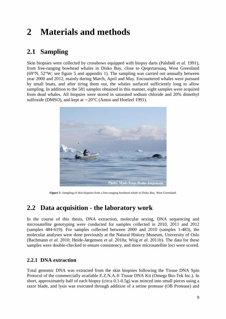
2.1 Sampling Skin biopsies were collected by crossbows equipped with biopsy darts (Palsbøll et al. 1991), from free-ranging bowhead whales in Disko Bay, close to Qeqertarsuaq, West Greenland (69°N, 52°W; see figure 5 and appendix 1). The sampling was carried out annually between year 2000 and 2012, mainly during March, April and May. Encountered whales were pursued by small boats, and after tiring them out, the whales surfaced sufficiently long to allow sampling. In addition to the 581 samples obtained in this manner, eight samples were acquired from dead whales. All biopsies were stored in saturated sodium chloride and 20% dimethyl sulfoxide (DMSO), and kept at −20°C (Amos and Hoelzel 1991).

Figure 5: Sampling of skin biopsies from a free-ranging bowhead whale in Disko Bay, West Greenland.

2.2 Data acquisition - the laboratory work In the course of this thesis, DNA extraction, molecular sexing, DNA sequencing and microsatellite genotyping were conducted for samples collected in 2010, 2011 and 2012 (samples 484-619). For samples collected between 2000 and 2010 (samples 1-483), the molecular analyses were done previously at the Natural History Museum, University of Oslo (Bachmann et al. 2010; Heide-Jørgensen et al. 2010a; Wiig et al. 2011b). The data for these samples were double-checked to ensure consistency, and more microsatellite loci were scored.

2.2.1 DNA extraction

Total genomic DNA was extracted from the skin biopsies following the Tissue DNA Spin Protocol of the commercially available E.Z.N.A.® Tissue DNA Kit (Omega Bio-Tek Inc.). In short, approximately half of each biopsy (circa 0.1-0.5g) was minced into small pieces using a razor blade, and lysis was executed through addition of a serine protease (OB Protease) and

10

TL Buffer at 55°C for at least three hours. During incubation, the samples were vortexed every 30 minutes. If lysis proceeded overnight, the samples were vortexed well prior to incubation. Afterwards, insoluble debris was pelleted by short centrifugation (Eppendorf Centrifuge 5417 C). BL Buffer and ethanol were added to precipitate the DNA, before the DNA was bound to a HiBind DNA Mini Column through centrifugation. After washing the column with the buffers HB and DNA Wash, the DNA was eluted by adding 100 µL Elution Buffer again followed by centrifugation. This last step was carried out twice, which according to the protocol would elute about 90% of the DNA bound to the column. The obtained concentration of the DNA was not explicitly estimated, but earlier studies following the same protocol yielded concentrations of about ~50-100 ng/µL (Bachmann, pers. comm. 2012). It was assumed that the yields of the DNA extractions of this thesis were in the same order of magnitude. After the DNA extraction, the remaining half of each biopsy was again stored in saturated sodium chloride and 20% DMSO and kept frozen, serving as a backup.

2.2.2 Molecular sexing

Molecular sex determination was accomplished through a PCR based approach, as published by Palsbøll et al. (1992) and Bérubé and Palsbøll (1996). 540 nucleotides of the last exon in the ZFX/ZFY gene were amplified using 1 µL of each of the primers ZFYX0582 and ZFYX1204 (Eurofins MWG Operon, 10µM; see appendix 2), 7.5 µL AmpliTaq Gold® PCR Master Mix (Applied Biosystems®), 4.5 µL ultrapure H2O (provided through Direct-Q™ Progard® (Millipore™)) and 1 µL extracted DNA; constituting a total volume of 15 µL in each PCR reaction. Four of the samples did not yield amplification products using this protocol. For these samples, an additional bead PCR using illustra™ PuReTaq™ Ready-To-Go™ PCR beads (GE Healthcare) was done. The beads were combined with 1 µL of each primer, 21 µL ultrapure H2O and 2 µL DNA, and the PCR was carried out in a thermal cycler (GeneAmp® PCR System 9700 (Applied Biosystems®) or T100™ Thermal Cycler (Bio-Rad Laboratories, Inc.)). The PCR protocol consisted of an initial denaturation at 94°C for 2 minutes, followed by 35 cycles of 94°C for 30 seconds, 51°C for 20 seconds and 72°C for 30 seconds, and a final extension at 72°C for 3 minutes. Restriction of the obtained PCR products was conducted with the restriction endonuclease OliI (AleI, PureExtreme® (Fermentas®)), incubating 1.5 µL (~15 units) combined with 1 µL Buffer R (PureExtreme® (Fermentas®)) and 12 µL of the obtained PCR products for one hour at 37°C. After the incubation, 5 µL of loading buffer were added, and the samples were run on a 1% agarose gel stained with GelRed™ Nucleic Acid Gel Stain (Biotium). The gels were visualized using the Gel Logic 200 Imaging System (Kodak) and the computer program KODAK MI APPLICATION (Molecular Imaging Systems Eastman Kodak), and the restriction fragments were compared against a length standard (λ DNA/EcoRI + HindIII (Fermentas®) or FastRuler™ Low Range DNA Ladder (Fermentas®)). For an example, see figure 6.

Figure 6: Example of molecular sex determination by utilizing a restriction endonuclease (OliI) on a fragment of the ZFX and ZFY genes. The males exhibit two bands visualized by gel electrophoresis, whereas the females show one band. The FastRuler™ Low Range DNA Ladder was used as a length standard (“L” in the figure), indicating the fragment sizes in base pairs (bp).

11

2.2.3 Sequencing of the mitochondrial D-loop region

A stretch of 453 base pairs of the mitochondrial D-loop region (position 15 473- 15 925 in the complete mitochondrial genome of the bowhead whale (Arnason et al. 1993, GenBank Accession no. AP006472 (Sasaki et al. 2005)), was amplified and sequenced for each sample. Amplification was carried out through PCR with a reaction volume of 15 µL, consisting of 7.5 µL PCR-mix (AmpliTaq Gold® PCR Master Mix (Applied Biosystems®)), 1 µL of each primer (mt19 and mt20, 10µM (MWG-Biotech AG); see appendix 2), 1 µL of ultrapure H2O and 1 µL extracted genomic DNA.

PCR was performed using a thermal cycler, in accordance to a protocol of initial denaturation at 94°C for 3 min followed by 35 cycles with denaturation at 94°C for 30 seconds, annealing at 52°C for 20 seconds and synthesis at 72°C for 30 seconds, and a final elongation step at 72°C for 3 minutes, before the samples were stored at 4°C.

To eliminate unincorporated dNTPs and excess primers prior to sequencing of the PCR product, 4 µL of 10 times diluted ExoSAP-IT® (Affymetrix® (USB Products®)) were added to the PCR products, and were incubated at 37°C for 30 minutes. After this treatment, the temperature was raised to 65°C for 15 minutes, inactivating the hydrolytic enzymes in ExoSAP-IT.

The samples were shipped to StarSEQ® GmbH, Mainz, Germany, for sequencing. To ensure that the required amount of PCR product could be provided, the concentration of a subset of samples was measured utilizing a spectrophotometer (Pico100 (Picodrop™)). The concentrations were found to be between 325 and 360 ng/µL. A sufficient volume of 1 µL of each PCR product was mixed with 5 µL ultrapure H2O and 1 µL of either primer mt19 or mt20 and sent to StarSEQ® GmbH at ambient temperature.

Eight samples were however sequenced at the DNA laboratory of Natural History Museum, Oslo, Norway, in accordance to the protocol of BigDye® Terminator v3.1 Cycle Sequencing Kit (Applied Biosystems®). Two µL of the ExoSAP-IT treated PCR products were mixed with 1 µL of either mt19 or mt20, 2 µL of BigDye v3.1, 2 µL of BigDye 5X Sequencing Buffer and 3 µL of ultrapure H2O, constituting 10 µL as a final volume for each reaction. The sequencing PCR took place in a thermal cycler, with an initial denaturation at 94°C for 3 minutes, followed by 35 cycles with 94°C for 30 seconds, 52°C for 20 seconds and 60°C for 4 minutes, and a 3 minute final extension step at 60°C. As recommended by the manufacturers, unincorporated dye terminators were removed. This was done by adding 1 µL of 3M sodium acetate (Merck KGaA) and 25 µL of 100% ethanol to each well and incubating for 15 minutes on ice, before centrifuging the plate for 15 minutes at 2608 RCF in a plate centrifuge (Rotanta 46 RS (Andreas Hettich GmbH & Co. KG)). A pellet containing the DNA formed in the bottom of the wells, and an additional spinning at 14 RCF for 20 seconds with the plate inverted removed the excess liquid. After adding 100 µL of 70% ethanol, the spinning steps were repeated to further purify the sequence PCR products. Finally, 10 µL of Hi-Di™ Formamide (Applied Biosystems®) were added to each well to re-suspend the samples and to stabilize single stranded DNA, before capillary electrophoresis was carried out on the ABI prism 3130xl Genetic Analyzer (Hitachi, Applied Biosystems®), using 36 cm Capillary Array (Applied Biosystems®). The data was collected using the program FOUNDATION DATA COLLECTION v3.0 (Applied Biosystems®), and the obtained sequences were edited and aligned using the software BIOEDIT SEQUENCE ALIGNMENT EDITOR v7.0.5.3 (Hall 1999) and MEGA v5.05 (Tamura et al. 2011).

12

2.2.4 Genotyping microsatellite loci

The samples were genotyped for twelve microsatellite loci (Huebinger et al. 2008). Before the high-throughput scoring commenced, multiplexing attempts were carried out. The following loci were mainly successfully amplified and scored together: Bmy19/Bmy32; Bmy42/Bmy52/Bmy33; Bmy16/Bmy26; Bmy41/Bmy58; Bmy38/Bmy61. Bmy29 was amplified and genotyped alone.

The PCRs took place in the abovementioned thermal cyclers, and consisted of the components listed in table 1.

Table 1: Components of the PCR used for genotyping bowhead whales at 12 microsatellite loci. The samples were collected between year 2000 and 2012 in Disko Bay, West Greenland.

One locus (BmyA) Two loci (BmyA, BmyB) Three loci (BmyA, BmyB, BmyC)

Extracted DNA 1 µL 1 µL 2 µL

Primers (~10µM) BmyA forward 1 µL 1 µL 1 µL

BmyA reverse 1 µL 1 µL 1 µL

BmyB forward 1 µL 1 µL

BmyB reverse 1 µL 1 µL

BmyC forward 1 µL

BmyC reverse 1 µL

Ultrapure H20 2 µL Amplitaq Gold® 5 µL 5 µL 7 µL

Total volume 10 µL 10 µL 15 µL

One of the primers for each locus (DNA Technology A/S; see appendix 2) was fluorescently labeled, in order to visualize the alleles using a capillary electrophoresis. 1 µL of the PCR products were transfered to a an Optical 96-well Reaction Plate (Applied Biosystems®), and 0.3 µL Rox™ Size Standard (GeneScan™-500 (Applied Bioystems®)) were added to each well. To stabilize single stranded DNA, 9 µL Hi-Di™ Formamide (Applied Biosystems®) were added. The capillary electrophoresis took place in an ABI prism 3130xl Genetic Analyzer (Hitachi, Applied Biosystems®), using 36 cm Capillary Array (Applied Biosystems®). The computer program RUN3130xl DATACOLLECTION v3.0 (2) (Applied Biosystems®) was applied to collect the data, and the obtained results were visualized using GENEMAPPER v4.0 (Applied Biosystems®) and scored manually as recommended by Bonin et al. (2004).

Earlier microsatellite runs for samples 1-483 were re-scored to ensure consistency throughout the data set. In addition, Bmy16, Bmy19 and Bmy61 were not previously scored, and genotyping of these loci was carried out on the samples excluding the assumed within-year recaptures from previous studies (Wiig et al. 2011b).

13

2.3 Statistical analyses For every statistical test, a significance level (α) of 0.05 was used as a threshold value for rejection of the null hypotheses.

2.3.1 Identifying recaptures

The probability of identity (𝑃(𝐼𝐷); the probability that two individuals drawn at random will have the same genotype (Paetkau and Strobeck 1994)) and the probability of identity among siblings (𝑃(𝐼𝐷)𝑠𝑖𝑏𝑠; the probability that two full siblings will have the same genotype by chance (Waits et al. 2001)) were calculated using GENALEX v6.5b3 (Peakall and Smouse 2006; In press), in order to determine the number of loci required for identification of individuals.

Recaptures were in a first attempt identified manually utilizing the sort function in EXCEL (Microsoft®). The sorting was conducted several times based on different criteria, such as mitochondrial haplotype or the most polymorphic and least erroneously scored microsatellite loci (i.e. Bmy19, Bmy26, Bmy29 and Bmy53; see appendix 3).

For an automated identification of recaptures, CERVUS v3.0.3 (Kalinowski et al. 2007) was used to identify matching microsatellite genotypes within samples displaying the same sex. In these comparisons of pairs of genotypes, mismatches at up to three loci were allowed, in order to prevent from overlooking recaptures due to genotyping errors and/or allelic drop out (Palsbøll et al. 1997; Waits and Leberg 2000). This comparison was done twice; first time excluding the least robustly amplifying loci Bmy32 and Bmy38 yielding a total of ten loci to be compared, while the minimum number of loci needed for match was set to seven and two mismatching loci were allowed. The second time the loci with an >2% error rate (i.e. Bmy32, Bmy38, Bmy41, Bmy58 and Bmy61) were left out, and a minimum of three loci were required for match whereas three mismatching loci were allowed. The suggested recaptures were manually compared regarding sex, microsatellite genotypes and mitochondrial haplotype, and systematically the anticipated true recaptures were revealed. A consensus microsatellite genotype was established for samples from the same individual and used in further analyses. Additionally, per locus error rates were estimated by comparing the alleles between the recaptures. In this way, ratios of differing replicated alleles to the total number of replicated alleles were procured by mere counting (the per-allele error rates; Morin et al. 2009).

In order to assess whether there are differences between the sexes in their tendency to revisit Disko Bay, the sex ratios in the recaptures and the aggregation as a whole were estimated and compared.

14

2.3.2 Population size estimation

The size of the bowhead whale population that supplies the Disko Bay aggregation with individuals was estimated for 2012 using the Chapman estimator (Chapman 1951; Chao and Huggins 2005; Wiig et al. 2011a; 2011b):

𝑁� = (𝑛1 + 1)(𝑛2 + 1)

(𝑚2 + 1) − 1

with a corresponding variance approximated as (Seber 1970):

𝑉𝑎𝑟(𝑁�) = (𝑛1 + 1)(𝑛2 + 1)(𝑛1 − 𝑚2)(𝑛2 −𝑚2)

(𝑚2 + 1)2(𝑚2 + 2)

where 𝑛1 is the number of unique individuals sampled in year 2000 to 2011, 𝑛2 is the number of individual whales sampled in 2012 and 𝑚2 is the number of recaptures in 2012, i.e. the number of unique individuals first sampled in the period 2000-2011 and subsequently resampled in 2012.

This was calculated for both sexes combined and for the females separately. The pertaining 95% confidence intervals (95% CI) were computed as 𝑁� ± 1.96�𝑉𝑎𝑟(𝑁�) .

Eight samples taken from dead whales (two males and six females) were excluded from the calculations, as they – by default – could not be recaptured.

An equivalent population size estimate for 2011 was obtained in the same manner.

2.3.3 Investigating possible cyclicity

To examine possible patterns of cyclicity between capture and recapture for the female bowhead whales in Disko Bay, the following equations (Wiig et al. 2011b) were applied to the samples of non-hunted females:

Under the null hypothesis of random recapture, the probability of recapturing a whale sampled in year y after j number of years (𝑝𝑦+𝑗) was estimated as:

�̂�𝑦+𝑗 = �𝑛𝑦𝑀𝑦+𝑗

� �𝑟𝑦+𝑗𝑛𝑦+𝑗

�

where 𝑛𝑦 is the number of whales sampled in year y, 𝑀𝑦+𝑗 is the number of unique individuals sampled before year y+j, 𝑟𝑦+𝑗 is the number of recaptures in year y+j and 𝑛𝑦+𝑗 is the number of whales sampled in year y+j.

15

The expected number of recaptures if there was no cyclicity (𝑟𝑗) was thereafter estimated as:

�̂�𝑗 = � �𝑛𝑦+𝑗 × �̂�𝑦+𝑗�2000≤𝑦≤2011

with summation over all years y. In order to evaluate possible cyclicity in the years between capture and recapture, the expected number of recaptures (�̂�𝑗) was compared to the observed number of recaptures for every j.

2.3.4 Investigating possible population substructure

CONVERTER (Glaubitz 2004) and DNASP v5.10.01 (Librado and Rozas 2009) were applied in order to convert the input files to the appropriate format required by other computer programs.

Analyses based on the mitochondrial haplotypes

Mitochondrial haplotype networks were established by NETWORK v4.6.1.0 (fluxus-engineering.com), using the median joining (Bandelt et al. 1999) and star contraction algorithms (Forster et al. 2001), and applying the MP postprocessing option (Polzin and Daneshmand 2003). The value of ɛ was set to 0 after empirically exploring various values, as recommended in the user manual. Additionally, transversions, transitions and indels were weighted differentially (3:1:2, respectively) in concordance with the guidelines in this manual.

Haplotype frequencies and molecular diversity indices were computed using ARLEQUIN v3.5.1.2 (see Excoffier and Lischer 2010 and references therein) for each year and for all the samples as an entirety. For the females sampled between 2005 and 2012, FSTs and AMOVA were further calculated in the program, and an exact test of differentiation between the sample years was performed.

Analyses based on the microsatellite loci

GENEPOP v4.0.10 (Raymond and Rousset 1995; Rousset 2008) was used to test for heterozygote deficiency, heterozygote excess and linkage disequilibrium among the microsatellite loci, while polymorphic information content (PIC) for each microsatellite locus was found through application of CERVUS v3.0.3 (Kalinowski et al. 2007). In order to detect evidence of stutter (caused by slippage during the PCR amplification) or scoring errors such as large allele dropout (i.e. short allele dominance) or null alleles (non-amplified alleles), the dataset was analyzed in the microsatellite data checker software MICRO-CHECKER v2.2.3 (van Oosterhout et al. 2004). Microsatellite markers exhibiting any of these characteristics were mainly excluded in the further analyses (i.e. Bmy38).

Allelic richness and private allelic richness were calculated for each year (with N≥20; 2005-2012) by rarefaction using the computer program HP-RARE v1.1 (Kalinowski 2005), to compensate for differences in sample size (Kalinowski 2004). In pursuance of testing the null hypothesis “each sampling year have the same number of unique alleles”, a two-sided sign test across all loci was used in R v2.11.1 (R Development Core Team 2010), as suggested by Kalinowski (2004).

16

To assess the decrease of heterozygosity due to inbreeding (Wright 1922; Weir and Cockerham 1984), the inbreeding coefficient FIS was estimated for each sampling year (2005-2012) with the program FSTAT v2.9.3.2 (Goudet 2001). Additionally for the females sampled between 2005 and 2012, AMOVA was computed by ARLEQUIN v3.5.1.2, and global FIS-, FIT- and FST- as well as pairwise FST-values were obtained. Possible genetic differentiation between pairs of sampling years was traced by applying an exact test of differentiation with the same software, and tests for Hardy-Weinberg disequilibrium were performed.

Possible genetic structuring of the females sampled in Disko Bay was examined using the software STRUCTURE v2.3.4 (Pritchard et al. 2000; Falush et al. 2003). In this software, clusters of individuals that are not in Hardy-Weinberg or linkage disequilibrium are identified by assigning individuals to clusters based on their multilocus genotype. The microsatellite locus Bmy38 was removed from the dataset, due to the presence of null-alleles and extensive linkage disequilibrium. Burn-in and Markov chain Monte Carlo (MCMC) simulations were set to 100 000 steps each (Gilbert et al. 2012), and the estimated number of clusters (K) ranged from 1 to 8. This was conducted for the females sampled each year between 2005 and 2012. Analyses of the females excluding every between-year recapture and avoiding all loci in Hardy-Weinberg and linkage disequilibrium were additionally commenced; i.e. only Bmy19, Bmy26, Bmy29, Bmy41 and Bmy58 were analyzed (see appendix 3). For every run, the correlated allele frequencies model and the admixture models were applied, which are believed to be the most likely scenarios biologically (Martien et al. 2007). The correlated allele frequency model assumes that the allele frequencies in the putative clusters are similar due to migration or shared ancestry, while the admixture model allows for the individuals to have mixed ancestry from the K clusters. In order to estimate K, the K with the maximum log probability of the data, is chosen (Pritchard et al. 2000). However, as recognized by the authors of the program (Pritchard et al. 2000), STRUCTURE relies on ad hoc procedures and careful interpretation of K is required. Evanno et al. (2005) therefore further improved STRUCTURE’s ability to detect the real K, founded on the rate of change in the log probability of the given data as K increases (ΔK). By using an R script handling these operations (Ehrich 2006; Ehrich et al. 2007), expanded information upon the temporal structure between the sampling years in Disko Bay was obtained.

In order to reveal family groups, the individual genotypes were analyzed in the software COLONY v2.0.2.3 (Jones and Wang 2009), in which full-pedigree likelihood methods are implemented to jointly infer parentage and sibship. Male and female polygamy were tolerated, and inbreeding was additionally not excluded. As the software allows for a certain degree of incorrect allele scoring, the error rates previously estimated were provided. In an exploratory analysis, eight of the microsatellite loci among all the individuals were investigated, excluding the loci in Hardy-Weinberg disequilibrium (i.e. Bmy33, Bmy38 and Bmy61, see appendix 3). The probability of finding the parents among the candidate samples were guesstimated as 0.3, based on the ratio of sampled females to the estimated female population size. As very little data exist on the size and age of the sampled whales, all individuals were possible offspring and in either in the candidate mother or candidate father samples according to their sex. This is feasible when no close inbreeding exists and an individual appears only once in each family group (i.e. as either a parent or an offspring; Wang and Santure 2009), which thus is assumed to be valid for the samples during this analyses. An additional search for siblings was performed excluding the males, in order to illuminate possible female family groups.

17

3 Results A total of 589 samples were included in the dataset displaying the assigned sex, mitochondrial haplotype and microsatellite genotype, when the previously obtained data for sample 1 to 483 were added. Molecular sexing was successfully accomplished for all individuals, while mitochondrial haplotype determination failed for six individuals. Fifty-two distinct haplotypes were observed. For the microsatellites, the per locus error rates ranged from 0.3-6.7% (when assuming correct scoring of one of the disaccording alleles; see appendix 3). Visualization of the Bmy32 alleles displayed a variable stuttering pattern which obscured reliable scoring, and this locus was therefore abandoned as a marker in this study. Thus, 11 microsatellite loci were targeted and examined in the subsequent analyses.

The number of alleles per microsatellite locus varied between eight (Bmy16) and 33 (Bmy29), with a mean polymorphic information content (PIC) of 0.8427 ranging from 0.6976 (Bmy16) to 0.9373 (Bmy29) among the loci (see appendix 3). Linkage disequilibrium was found significant among several pairs of loci (see appendix 3). Further, a possible presence of null alleles and stuttering were discovered for Bmy38. However, there were no additional signs of stuttering or null alleles for the other loci, nor was any large allele dropout evident.

3.1 Recaptures For each microsatellite locus, 𝑃(𝐼𝐷) ranged between 0.1090 (Bmy16) and 0.0067 (Bmy29), consequently yielding a probability of identity between two individuals of <0.01 when combining two loci (see appendix 3). A more conservative estimate was given by 𝑃(𝐼𝐷)𝑠𝑖𝑏𝑠, where the corresponding locus-specific probabilities of identity between siblings varied from 0.4083 (Bmy16) to 0.2814 (Bmy29), requiring five loci to achieve probability of identity <0.01.

Accordingly, 142 of the 589 samples were considered within-year duplicates of an individual and were not included in further analyses. In addition, there were 46 between-year recaptures; of which one male was captured in three different years (see table 2). Thus, 401 unique individuals were recognized (83 males, 317 females and one of unknown sex), and 393 of these samples were collected from living, free-ranging whales. Hence, the proportion of females calculated over all sampling years was 79%, while the females constituted 83% of the between-year recaptures.

18

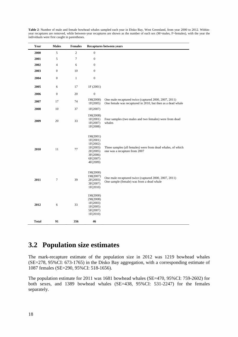
Table 2: Number of male and female bowhead whales sampled each year in Disko Bay, West Greenland, from year 2000 to 2012. Within-year recaptures are removed, while between-year recaptures are shown as the number of each sex (M=males, F=females), with the year the individuals were first caught in parentheses.

Year Males Females Recaptures between years

2000 5 2 0

2001 5 7 0

2002 4 6 0

2003 0 10 0

2004 0 1 0

2005 6 17 1F (2001)

2006 0 20 0

2007 17 74 1M(2000) 1F(2005)

One male recaptured twice (captured 2000, 2007, 2011) One female was recaptured in 2010, but then as a dead whale

2008 10 37 1F(2007)

2009 20 33

1M(2008) 1F(2001) 1F(2007) 1F(2008)

Four samples (two males and two females) were from dead whales

2010 11 77

1M(2001) 1F(2001) 1F(2002) 1F(2003) 2F(2005) 3F(2006) 6F(2007) 4F(2009)

Three samples (all females) were from dead whales, of which one was a recapture from 2007

2011 7 39

1M(2000) 1M(2007) 2F(2003) 3F(2007) 1F(2010)

One male recaptured twice (captured 2000, 2007, 2011) One sample (female) was from a dead whale

2012 6 33

1M(2000) 2M(2008) 1F(2003) 1F(2005) 5F(2007) 1F(2010)

Total 91 356 46

3.2 Population size estimates The mark-recapture estimate of the population size in 2012 was 1219 bowhead whales (SE=278, 95%CI: 673-1765) in the Disko Bay aggregation, with a corresponding estimate of 1087 females (SE=290, 95%CI: 518-1656).

The population estimate for 2011 was 1681 bowhead whales (SE=470, 95%CI: 759-2602) for both sexes, and 1389 bowhead whales (SE=438, 95%CI: 531-2247) for the females separately.

19

3.3 Cyclicity As the observed numbers of recaptures after j number of years were compared with the expected values if no cyclicity was present (see table 3), a trend of more recaptures than expected were revealed after 4, 5 and 8 years, while there were fewer recaptures than expected after 2, 3 and 6 years. After 1, 7, 9, 10, 11 and 12 years, the observed numbers of recaptures were similar to the expected numbers.

Table 3: Estimated probability of recapture (𝒑�𝒚+𝒋) after j years, for a female bowhead whale first captured in year y in Disko Bay, West Greenland, between year 2000 and 2011 (in italics). The expected numbers of recaptures (𝒓�𝒚+𝒋 = 𝒏𝒚+𝒋 𝐱 𝒑�𝒚+𝒋) are listed below their corresponding 𝒑�𝒚+𝒋. For each j, the expected recaptures are added over all years y, and the pertaining observed numbers of recaptures are given.

Number of years to recapture (j) Mark year (y) 1 2 3 4 5 6 7 8 9 10 11 12

2000 0 0 0 0 0.0045 0 0.0004 0.0004 0.0011 0.0023 0.0012 0.0017 N=2 0 0 0 0 0.0769 0 0.0323 0.0149 0.0353 0.1717 0.0471 0.0557

2001 0 0 0 0.0158 0 0.0015 0.0014 0.0040 0.0081 0.0043 0.0059 N=7 0 0 0 0.2692 0 0.1129 0.0522 0.1235 0.6010 0.1647 0.1951

2002 0 0 0.0136 0 0.0013 0.0012 0.0034 0.0070 0.0037 0.0051 N=6 0 0 0.2308 0 0.0968 0.0448 0.1059 0.5152 0.1412 0.1672

2003 0 0.0226 0 0.0022 0.0020 0.0057 0.0116 0.0062 0.0084 N=10 0 0.3846 0 0.1613 0.0746 0.1765 0.8586 0.2353 0.2787

2004 0.0023 0 0.0022 0.0002 0.0006 0.0012 0.0006 0.0008 N=1 0.0385 0 0.0161 0.0075 0.0176 0.0859 0.0235 0.0279

2005 0 0.0038 0.0034 0.0097 0.0197 0.0105 0.0144 N=17 0 0.2742 0.1270 0.3000 1.4596 0.4000 0.4739

2006 0.0044 0.0040 0.0114 0.0232 0.0124 0.0169 N=20 0.3226 0.1493 0.3529 1.7172 0.4706 0.5575

2007 0.0147 0.0416 0.0847 0.0452 0.0617 N=73 0.5448 1.2882 6.2680 1.7176 2.0348

2008 0.0211 0.0429 0.0229 0.0313 N=37 0.6529 3.1768 0.8706 1.0314

2009 0.0360 0.0192 0.0262 N=31 2.6616 0.7294 0.8640

2010 0.0458 0.0625 N=74 1.7412 2.0627

2011 0.0321 N=39 1.0592

Sum of recaptures Expected (r̂ j) 7.0208 8.0652 8.7291 5.2042 4.2310 1.3775 1.5464 0.9168 1.0562 0.5037 0.2422 0.0557 Observed 7 3 5 7 7 0 2 4 2 0 0 0

20

3.4 Population substructuring

3.4.1 Mitochondrial analyses

Two median joining networks of the mitochondrial D-loop region were established (figure 7), showing the relative frequencies of the haplotypes and the genetic relationships between them. The first network illustrates the number of assumed mutations between the haplotypes and excludes the between-year recaptures in the frequency calculations (figure 7a), while the second more simplified network shows the frequencies of the haplotypes in each sampling year (figure 7b). The absolute frequencies of the haplotypes are given in appendix 4, while the segregating sites are listed in appendix 5. Of the 52 haplotypes, DB-4 was the most common haplotype, with a frequency of 20.8% of all individuals. Small differences in haplotype frequencies were yet found between the sampling years. The frequencies of DB-4 and DB-10 were approximately equal in 2007, while DB-4 was nearly four times as frequent as DB-10 in 2010. Additionally, DB-6 was about four times as frequent in 2008 as in 2007. Sixteen unique haplotypes were discovered, scattered evenly among the sampling years. Accordingly, no obvious patterns consistent with a temporal substructure could be deduced from the haplotype frequencies among the sampling years.

The haplotypic molecular diversity is presented in appendix 6. A total of 44 segregating sites were found among all haplotypes; there were observed 38 transitions, eight transversions and one site with an indel.

The analysis of molecular variance (AMOVA) for the females sampled between 2005 and 2012 revealed that the covariance component of the total molecular variance due to differences within the sampling years was substantially higher than the covariance component due to differences between sampling years (table 4). FST was further tested by 1023 permutations of haplotypes among these females, yielding a significant result. (FST=0.02178, P=0.00391 ± 0.00185). However, pairwise FST among pairs of sampling years was significant only for comparisons including 2007, 2008 and 2010 (table 5). An exact test of differentiation between the sampling years 2005-2012 analyzing the females rendered significance for eight pairs of sampling years (100 000 Markov steps done, see table 6). A significant P-value (P=0.03673±0.02820) for non-differentiation was obtained for an exact global test among the females in the sampling years 2005-2012.

Table 4: Analysis of molecular variance of the mitochondrial D-loop haplotypes in female bowhead whales, sampled in Disko Bay, West Greenland, between 2005 and 2012. Differential weighting of the transitions and transversions (1:3, respectively) was applied during the statistical analysis.

Source of Sum of Variance Percentage

variation d.f. squares components of variation

Among sampling years 7 36.369 0.06187 Va 2.18

Among individuals within sampling years 316 878.338 2.77955 Vb 97.82

Total 323 914.707 2.84143

21

Table 5: Pairwise FST-values between pairs of sampling years (below diagonal) and a matrix of significant FST P-values (above diagonal; + indicates significant P-value, - indicates non-significance). This was obtained by analyzing the mitochondrial D-loop haplotypes in female bowhead whales, sampled in Disko Bay, West Greenland, between year 2000 and 2012. Differential weighting of the transitions and transversions (1:3, respectively) was applied during the statistical analysis.

2000 2001 2002 2003 2004 2005 2006 2007 2008 2009 2010 2011 2012

2000 - - - - - - - - - - - -

2001 -0.01648 - - - - - - - - - - -

2002 -0.27007 -0.08686 - - - - - + - - - -

2003 0.20515 -0.05912 0.08865 - - - - - - - - -

2004 -1.00000 0.44118 0.08444 0.63810 - - - + - - - -

2005 -0.05835 -0.07601 -0.04183 -0.01459 0.38333 - - - - - - -

2006 0.14361 -0.04392 0.05921 -0.00414 0.54515 -0.00586 - - - - - -

2007 -0.08610 -0.04242 -0.05974 0.02470 0.25524 -0.01520 0.02591 + + + - -

2008 0.25821 -0.00538 0.13621 0.04264 0.64251 0.03667 -0.00437 0.08249 - + - +

2009 0.11642 -0.03903 0.03758 0.02849 0.52800 -0.00138 0.00842 0.05060 0.00157 - - -

2010 0.17253 -0.03469 0.06588 0.00025 0.57880 -0.01360 -0.00873 0.03694 0.02294 0.01118 - +

2011 0.04102 -0.06935 -0.00864 -0.00341 0.44890 -0.01918 -0.00429 0.01705 0.00850 -0.00813 0.00519 -

2012 -0.14360 -0.03715 -0.06397 0.03708 0.22716 -0.02073 0.03349 -0.00539 0.07625 0.02898 0.04412 0.00667

Table 6: An exact test of differentiation between all pairs of sampling years for female bowhead whales in Disko Bay, sampled between year 2000 and 2012, by analyzing the mitochondrial D-loop region. The non-differentiation exact P-values are listed below the diagonal, while the matrix of significance for these P-values is given above the diagonal (+ indicates significant P-value, - indicates non-significance). Differential weighting of the transitions and transversions (1:3, respectively) was applied during the statistical analysis.

2000 2001 2002 2003 2004 2005 2006 2007 2008 2009 2010 2011 2012

2000

- - - - - - - - - + - -

2001 1.00000± 0.0000

- - - - - - - - - - -

2002 0.58056± 0.0064

1.00000± 0.0000

- - - - - - - - - -

2003 0.17305± 0.0067

0.67106± 0.0060

0.34230± 0.0086

- - - - - - - - -

2004 1.00000± 0.0000

1.00000± 0.0000

1.00000± 0.0000

0.36685± 0.0074

- - - - - - - -

2005 0.48471± 0.0118

0.83032± 0.0035

0.90268± 0.0040

0.63664± 0.0050

0.72184± 0.0152

- - - - - - -

2006 0.21790± 0.0077

0.57044± 0.0147

0.54107± 0.0087

0.13987± 0.0083

0.81534± 0.0126

0.85051± 0.0069

+ - - + - -

2007 0.07593± 0.0099

0.37450± 0.0128

0.94166± 0.0070

0.37334± 0.0178

0.79218± 0.0159

0.65518± 0.0216

0.02109± 0.0045

+ + - - -

2008 0.16579± 0.0095

0.34313± 0.0154

0.51921± 0.0082

0.34817± 0.0119

0.38726± 0.0102

0.36569± 0.0130

0.35554± 0.0118

0.02089± 0.0057

+ + - -

2009 0.06647± 0.0042

0.37392± 0.0132

0.67389± 0.0119

0.10770± 0.0070

0.59403± 0.0107

0.73764± 0.0033

0.25694± 0.0059

0.00103± 0.0007

0.04367± 0.0050

- - -

2010 0.02256± 0.0048

0.12517± 0.0092

0.64732± 0.0114

0.45401± 0.0137

0.65060± 0.0236

0.62557± 0.0183

0.04450± 0.0035

0.07807± 0.0082

0.01827± 0.0047

0.09280± 0.0071

+ -

2011 0.11193± 0.0090

0.85393± 0.0059

0.97439± 0.0031

0.92395± 0.0071

0.85991± 0.0099

0.39049± 0.0127

0.05721± 0.0046

0.07396± 0.0075

0.45438± 0.0146

0.13936± 0.0102

0.04005± 0.0044

-

2012 0.28278± 0.0123

0.65303± 0.0076

1.00000± 0.0000

0.46577± 0.0093

1.00000± 0.0000

0.97209± 0.0019

0.20617± 0.0087

0.13590± 0.0126

0.10752± 0.0068

0.56821± 0.0084

0.14252± 0.0111

0.56390± 0.0112

23

b

Figure 7: Median joining networks of the observed mitochondrial D-loop haplotypes of bowhead whales in Disko Bay, obtained through a 1:3:2 weighting of respectively transitions, transversions and indels. Black nodes are median vectors, which are hypothesized intermediate sequences. The lengths of the connective lines are proportional to the number of mutations between the connected haplotypes, while circle sizes are proportional to the number of samples. In figure a, the network also displays the number of mutations between the haplotypes, indicated by red dots. The absolute numbers of haplotype frequencies observed from 2000 to 2012 are listed in appendix 4. Figure b is obtained through a star contraction algorithm, and the color coding refers to different sampling years. All recaptures are removed in figure a, but in order to emphasize the haplotype frequencies in each sampling year, between-year recaptures are not removed from the latter network (figure b).

24

3.4.2 Microsatellite analyses

Using a pairwise sign-test across loci, private allelic richness was found to be similar among the sampling years analyzing both sexes (P-values=0.0654 - 1.0000). However, analyzing the females only, P-values were significant for 2005 when compared with 2007, 2010 and 2011 (P=0.0386 for all of the three pairs). The average allelic richness and private allelic richness over all loci are listed in table 7.

The AMOVA based on the number of different microsatellite alleles showed that the total molecular variation for the females primarily originated from within individual variation (see table 8), while the variation among sampling years contributed <<1% to the total variation.

Over all loci, the averaged F-statistics for the females from the sampling years 2005-2012 yielded the fixation indices FIS: -0.03392 and FST: 0.00024, none significantly different from 0 (P=1.0000±0.0000). FIS for each sampling year (table 9) indicated no overall pattern of inbreeding within the sampling years, and only sampling year 2010 (when analyzing both sexes) yielded a significant FIS-value, with 2.67% of 1760 randomizations having a smaller FIS than the observed value (data not shown). Bootstrapping over all loci and sampling years between 2005 and 2012 rendered 95% confidence intervals including 0 for both sexes and for the females only (95%CI: -0.003 - 0.009 and -0.015 - 0.017 respectively).

Table 7: Allelic richness and private allelic richness averaged over 11 microsatellite loci, obtained through rarefaction. Samples of bowhead whales collected between 2005 and 2012 in Disko Bay, West Greenland, were analyzed.

Both sexes Females

Allelic richness Private allelic richness Allelic richness Private allelic richness

2005 10.36 0.21 9.62 0.15

2006 10.98 0.45 10.39 0.48

2007 11.04 0.33 10.34 0.26

2008 10.39 0.24 9.81 0.27

2009 10.98 0.25 10.43 0.25

2010 10.88 0.25 10.32 0.22

2011 11.41 0.55 10.35 0.40

2012 10.49 0.31 9.85 0.26 Table 8: Analysis of molecular variance (AMOVA), obtained by using allele frequencies at 11 microsatellite loci, when analyzing female bowhead whales sampled between 2005 and 2012 in Disko Bay, West Greenland.

Source of Sum of Variance Percentage

variation d.f. squares components of variation

Among sampling years 7 19.461 0.00069 Va 0.02

Among individuals within sampling years 322 877.539 -0.09570 Vb -3.39

Within individuals 330 962.500 2.91667 Vc 103.37

Total 659 1859.500 2.82166

25

Table 9: FIS values over 11 microsatellite loci for bowhead whales sampled in Disko Bay, West Greenland, for each sampling year between 2005 and 2012.

2005 2006 2007 2008 2009 2010 2011 2012

FIS Both sexes -0.011 -0.005 -0.006 0.009 -0.017 -0.022 0.027 0.024

FIS Females -0.022 -0.005 -0.004 0.015 -0.009 -0.020 0.020 0.027

Table 10: Pairwise FST-values between pairs of sampling years (below diagonal), and matrix of significant FST P-values (above diagonal; + indicates significant P-value, - indicates non-significance), using the microsatellite data obtained from female bowhead whales sampled in Disko Bay, West Greenland, between 2005 and 2012.

2000 2001 2002 2003 2004 2005 2006 2007 2008 2009 2010 2011 2012

2000 - - - - - - - - - - - -

2001 -0.04016 - - - - - - - - - - -

2002 -0.06640 0.00222 - - - - - - - - - -

2003 -0.03137 0.00589 0.00204 - + - - - - - - -

2004 0.07455 -0.05078 -0.02279 -0.05257 - - - - - - - -

2005 -0.04050 0.00368 0.01216 0.02411 0.00613 - - + + - + -

2006 -0.04954 0.00493 0.00541 -0.00257 -0.02461 0.00197 - - - - - -

2007 -0.01122 -0.00294 0.00138 0.00566 -0.01078 0.00234 -0.00108 - - - - -

2008 0.01288 0.00724 0.01091 0.00402 -0.03437 0.00712 0.00017 0.00272 - - - -

2009 -0.02796 -0.00345 -0.01223 0.00718 -0.02496 0.01032 0.00238 0.00142 0.00281 - - -

2010 -0.03551 -0.00044 -0.00432 0.00273 -0.04213 0.00517 -0.00104 -0.00367 0.00130 -0.00167 - -

2011 -0.04202 0.00213 -0.00391 0.00024 -0.04633 0.00748 -0.00113 -0.00369 0.00012 -0.00421 0.00165 -

2012 -0.05325 -0.00288 0.00177 0.00093 -0.04649 0.00311 0.00351 -0.00494 0.00234 0.00325 0.00077 0.00129

The exact test of differentiation between paired sampling years for the females based on microsatellite genotypes did not detect any significant values. The exact P-value for non-differentiation was 0.47964±0.13301, applying a global test of differentiation among females in the sampling years 2005-2012 (100 000 Markov steps done). However, the pairwise FST among sampling years gave significant results for four of the pairwise comparisons (obtained through 1023 permutations, see table 10), of which year 2005 was included in all of the pairs.

The test of Hardy-Weinberg equilibrium was significant for Bmy33, Bmy38 and Bmy61 over all individuals in all sampling years, when all recaptures were removed. However, analyzing each sampling year individually, only some of the years were significantly out of Hardy-Weinberg equilibrium for some of the loci (table 11). The test for heterozygote deficit rendered significant results for loci Bmy33 and Bmy38, while no locus showed any significant heterozygote excess (table 12). Further, the global test of heterozygote deficiency and excess across all loci gave not significant results.

26

Table 11: Locus specific observed (HO) and expected (HE) heterozygosity in bowhead whales sampled in Disko Bay, West Greenland. The P-value obtained by the exact test of Hardy-Weinberg equilibrium, as well as the corresponding standard deviation (s.d.) are listed for each locus. To the left are the results over all sampling years (2000-2012) of both sexes, while the results obtained when analyzing the females sampled in the period 2005-2012 are listed in the middle part of the table. The sampling years exhibiting significant P-values when tested separately are listed to the right in the table.

Both sexes (2000-2012) Females (2005-2012) Significant years

HO HE P-value s.d. HO HE P-value s.d. both sexes females

Bmy16 0.75131 0.7389 0.11825 0.00031 0.75000 0.73960 0.16210 0.00031 2007 Bmy19 0.86327 0.85025 0.22912 0.00039 0.84672 0.84865 0.12015 0.00025 Bmy26 0.92172 0.91498 0.57094 0.00033 0.89931 0.91516 0.12652 0.00022 2009

Bmy29 0.95592 0.94175 0.57116 0.00027 0.95000 0.94387 0.98179 0.00009 2005

Bmy33 0.78100 0.77302 0.01642 0.00013 0.80000 0.77756 0.02027 0.00010 2007 Bmy38 0.78307 0.84910 0.00085 0.00003 0.77007 0.85416 0.00278 0.00005 2011 2011

Bmy41 0.91123 0.90913 0.06791 0.00017 0.90647 0.90471 0.57575 0.00020 2005, 2008 Bmy42 0.78005 0.77764 0.48271 0.00046 0.77193 0.77470 0.67981 0.00029 2002

Bmy53 0.89114 0.88187 0.10517 0.00025 0.88889 0.88017 0.13353 0.00030 Bmy58 0.95128 0.92696 0.08610 0.00016 0.94346 0.92674 0.16699 0.00023 2007 Bmy61 0.83598 0.82278 0.00987 0.00010 0.83813 0.82990 0.00671 0.00007 2008

Table 12: Heterozygote deficit and excess in 11 microsatellite loci, calculated from biopsies of individual bowhead whales sampled in Disko Bay, West Greenland, between 2000 and 2012.

Heterozygote deficit Heterozygote excess

P-value S.E. P-value S.E.

Bmy16 0.5275 0.0259 0.4726 0.0259

Bmy19 0.6665 0.0266 0.3335 0.0266

Bmy26 0.5329 0.0397 0.4671 0.0397

Bmy29 0.6723 0.0401 0.3277 0.0401

Bmy33 0.0014 0.0012 0.9986 0.0012

Bmy38 0.0005 0.0005 0.9995 0.0005

Bmy41 0.3325 0.0375 0.6675 0.0375

Bmy42 0.6376 0.0277 0.3624 0.0277

Bmy53 0.7696 0.0300 0.2304 0.0300

Bmy58 0.8424 0.0320 0.1576 0.0320

Bmy61 0.8159 0.0273 0.1841 0.0273

All loci 0.0603 0.0117 0.9397 0.0117

The STRUCTURE analysis of the females sampled in each year between 2005 and 2012 identified K=6 as the most likely number of clusters given the multilocus microsatellite genotypes. Further, the approach using the second order rate of change of the log likelihood function regarding K (Evanno et al. 2005) yielded the highest ΔK values for K=2, with K=4 as the second most likely number of clusters (see figure 8) However, the algorithm did not converge for K>1 (figure 9). Additionally, when assigning the individuals’ genomes to the cluster of origin, no obvious patterns among the sampling years were uncovered (for an average of 10 iterations of K=4 and K=2, see figure 10). K=1 was recognized as the most likely number of clusters when analyzing the females sampled between 2005 and 2012 excluding all recaptures and avoiding loci in linkage and Hardy-Weinberg disequilibrium, with non-convergence for K>1 (see figure 8 and figure 9). The ΔK value was however highest for K=7 when the approach by Evanno et al. (2005) was applied. The individual assignments to the clusters for K=4 and K=7 from this run are shown in figure 11.

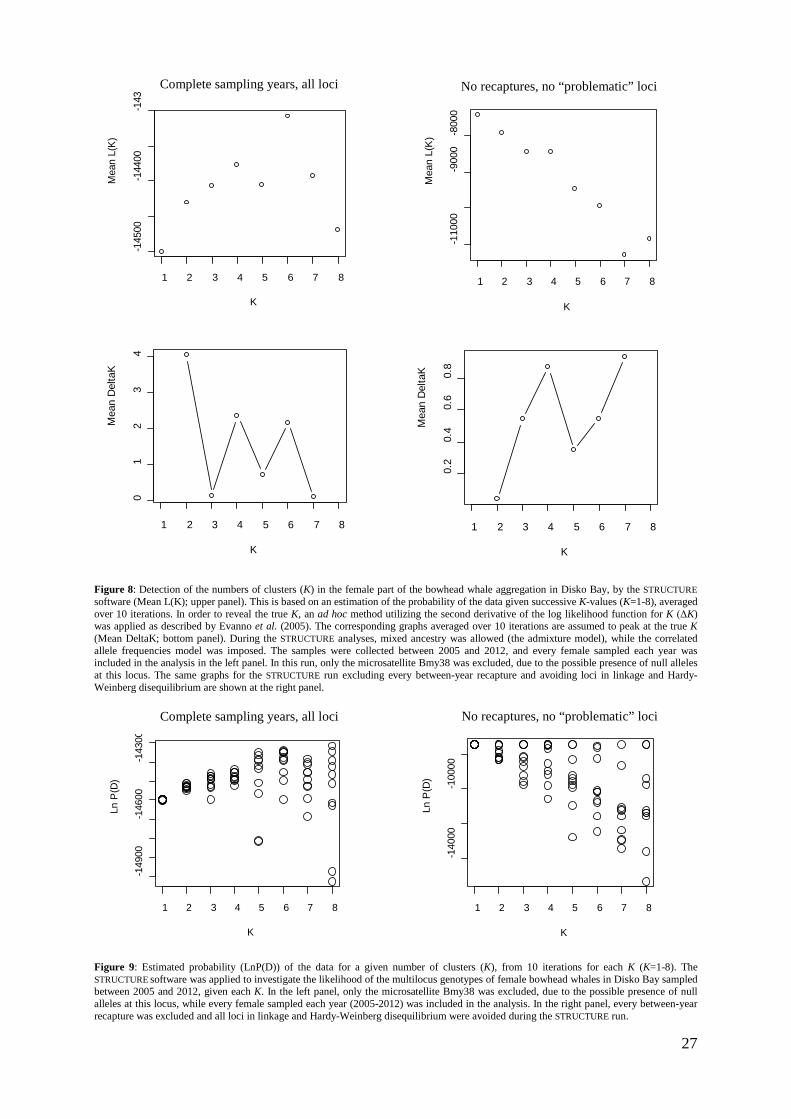
27

Figure 8: Detection of the numbers of clusters (K) in the female part of the bowhead whale aggregation in Disko Bay, by the STRUCTURE

software (Mean L(K); upper panel). This is based on an estimation of the probability of the data given successive K-values (K=1-8), averaged over 10 iterations. In order to reveal the true K, an ad hoc method utilizing the second derivative of the log likelihood function for K (ΔK) was applied as described by Evanno et al. (2005). The corresponding graphs averaged over 10 iterations are assumed to peak at the true K (Mean DeltaK; bottom panel). During the STRUCTURE analyses, mixed ancestry was allowed (the admixture model), while the correlated allele frequencies model was imposed. The samples were collected between 2005 and 2012, and every female sampled each year was included in the analysis in the left panel. In this run, only the microsatellite Bmy38 was excluded, due to the possible presence of null alleles at this locus. The same graphs for the STRUCTURE run excluding every between-year recapture and avoiding loci in linkage and Hardy-Weinberg disequilibrium are shown at the right panel.

Figure 9: Estimated probability (LnP(D)) of the data for a given number of clusters (K), from 10 iterations for each K (K=1-8). The STRUCTURE software was applied to investigate the likelihood of the multilocus genotypes of female bowhead whales in Disko Bay sampled between 2005 and 2012, given each K. In the left panel, only the microsatellite Bmy38 was excluded, due to the possible presence of null alleles at this locus, while every female sampled each year (2005-2012) was included in the analysis. In the right panel, every between-year recapture was excluded and all loci in linkage and Hardy-Weinberg disequilibrium were avoided during the STRUCTURE run.

1 2 3 4 5 6 7 8

-145

00-1

4400

-143

K

Mea

n L(

K)

1 2 3 4 5 6 7 8

-110

00-9

000

-800

0

K

Mea

n L(

K)

1 2 3 4 5 6 7 8

0.2

0.4

0.6

0.8

K

Mea

n D

elta

K

K

Ln P

(D)

1 2 3 4 5 6 7 8

-149

00-1

4600

-143

00

K

Ln P

(D)

1 2 3 4 5 6 7 8

-140

00-1

0000

1 2 3 4 5 6 7 8

01

23

4

K

Mea

n D

elta

K

Complete sampling years, all loci

Complete sampling years, all loci

No recaptures, no “problematic” loci

No recaptures, no “problematic” loci

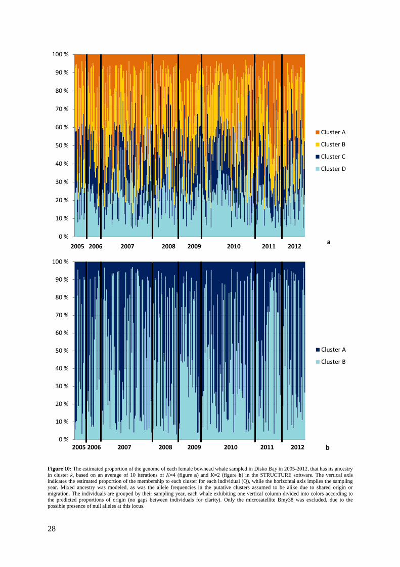
28

Figure 10: The estimated proportion of the genome of each female bowhead whale sampled in Disko Bay in 2005-2012, that has its ancestry in cluster k, based on an average of 10 iterations of K=4 (figure a) and K=2 (figure b) in the STRUCTURE software. The vertical axis indicates the estimated proportion of the membership to each cluster for each individual (Q), while the horizontal axis implies the sampling year. Mixed ancestry was modeled, as was the allele frequencies in the putative clusters assumed to be alike due to shared origin or migration. The individuals are grouped by their sampling year, each whale exhibiting one vertical column divided into colors according to the predicted proportions of origin (no gaps between individuals for clarity). Only the microsatellite Bmy38 was excluded, due to the possible presence of null alleles at this locus.

0 %

10 %

20 %

30 %

40 %

50 %

60 %

70 %

80 %

90 %

100 %

2005 2006 2007 2008 2009 2010 2011 2012

Cluster A

Cluster B

Cluster C

Cluster D

a

0 %

10 %

20 %

30 %

40 %

50 %

60 %

70 %

80 %

90 %

100 %

2005 2006 2007 2008 2009 2010 2011 2012

Cluster A

Cluster B

b

29

Figure 11: The estimated proportion of the genome of each female bowhead whale sampled in Disko Bay in 2005-2012, that has its ancestry in cluster k, based on an average of 10 iterations of K=4 (figure a) and K=7 (figure b) in the STRUCTURE software. The vertical axis indicates the estimated proportion of the membership to each cluster for each individual (Q), while the horizontal axis implies the sampling year. Mixed ancestry was modeled, as was the allele frequencies in the putative clusters assumed to be alike due to shared origin or migration. The individuals are grouped by their sampling year, each whale exhibiting one vertical column divided into colors according to the predicted proportions of origin (no gaps between individuals for clarity). To avoid linkage and Hardy-Weinberg disequilibrium among the markers, only the microsatellite loci Bmy19, Bmy26, Bmy29, Bmy41 and Bmy58 were analyzed in this run. Every between-year recapture was removed from the year of recapture.

0 %

10 %

20 %

30 %

40 %

50 %

60 %

70 %

80 %

90 %

100 %

2005 2006 2007 2008 2009 2010 2011 2012

Cluster A

Cluster B

Cluster C

Cluster D

0 %

10 %

20 %

30 %

40 %

50 %

60 %

70 %

80 %

90 %

100 %

2005 2006 2007 2008 2009 2010 2011 2012

Cluster A

Cluster B

Cluster C

Cluster D

Cluster E

Cluster F

Cluster G

a

b

30

The family group analyses by COLONY identified close relatedness among several of the bowhead whales in Disko Bay (1500 and more than 1000 half-sibling pairs were suggested in the runs; including and excluding the males respectively). When parentage was inferred, no mothers were identified but two of the males were assumed to each have sired two or more offspring. The different runs suggested similar number of full-sibling pairs (15 and 17 for both sexes and the females respectively), although the identification of the sibling pairs was not consistent among the runs (see figure 12).

Figure 12: Inferred sibship among the bowhead whales sampled in Disko Bay between 2000 and 2012, using the software COLONY. The individuals are placed at the x- and the y-axis (not all individuals are indicated with a line, for clarity). Only the microsatellite loci in Hardy-Weinberg equilibrium were analyzed (i.e.Bmy16, Bmy19, Bmy26, Bmy29, Bmy41, Bmy42, Bmy53 and Bmy58).

Females Both sexes

31

4 Discussion In this thesis, skin biopsies sampled from bowhead whales during the annual spring aggregation in Disko Bay, West Greenland, between year 2000 and 2012 were analyzed. The major aims were to obtain an updated population size estimate and to reveal female cyclicity in the revisits to the bay. Additionally, genetic substructuring of the population was assessed in order to address if different groups of related individuals visit the bay in different years.

Annual aggregations of bowhead whales have been observed during winter/spring in Disko Bay, West Greenland, since the 18th century (Eschricht and Reinhardt 1861). As the aggregations mainly consist of mature females that hardly ever are accompanied by calves, it is believed that Disko Bay primarily serves as a productive feeding ground for pregnant or post-lactating females, and possibly as a mating ground (Heide-Jørgensen et al. 2007; Laidre et al. 2007; Stafford et al. 2008; Tervo et al. 2009; Heide-Jørgensen et al. 2010a). If true, a cyclicity in the females’ migration to Disko Bay may be expected (Heide-Jørgensen et al. 2010a; Wiig et al. 2011b).

4.1 Recaptures Of the 589 bowhead whale biopsies sampled in Disko Bay between 2000 and 2012, 142 uninformative within-year recaptures were removed. Further, 46 between-year recaptures were recognized, resulting in a total of 401 unique individuals identified over the sampling period spanning from year 2000 to 2012. The between-year recaptures confirms that individual whales revisit the bay in different years (Eschricht and Reinhardt 1861). In order to assess if the revisits indicate a complex multiyear migration pattern (Heide-Jørgensen et al. 2010a; Wiig et al. 2011b), correct identification of the individuals is crucial. As the estimated scoring errors of the microsatellites are low (seven of the loci had an error rate of <2%, see appendix 3) and within the same range as previous reported error rates (Morin et al. 2009; Givens et al. 2010), matching genotypes rendered substantial confidence in uncovering recaptures. The probability of revealing all true recaptures was further enhanced by the flexibility of CERVUS, the software applied to identify recaptures, to allow for some mis-scoring, and the manual sorting on “reliable” microsatellite loci during the re-identification. Using the same methods and partly the same dataset as Bachmann et al. (2010), the error rates they obtained by control experiments of molecular sexing and sequencing of the mitochondrial control region are expected to be valid also for this study. The control experiments detected no discrepancies, and the authors thus reported an error rate of <0.5% for the molecular sexing and <2% for the mitochondrial DNA sequencing. In the current study, matching sex and mitochondrial haplotypes validated the findings of recaptures through the microsatellites. However, four pairs of identical microsatellite genotypes, with more than eight loci included, were not considered as originating from the same individuals, as the mitochondrial haplotype differed with more than one nucleotide. Acknowledging the 𝑃(𝐼𝐷)𝑠𝑖𝑏𝑠 of <0.01 when evaluating five loci, these identities are highly unlikely, and may constitute a source of errors in the further analyses. The impact of this uncertainty may not be severe, as only two pairs of these genotypes suggest between-year recaptures. However, rescoring of the microsatellites, sex and mitochondrial haplotype was still desired, but was abandoned in this study due to time limitations.

32

Genetic linkage would additionally increase the probability of misinterpreting similar genotypes as recaptures, and as the absence of linkage is an essential assumption in most genetic tests, it could also affect the other analyses performed in this thesis. While the analysis using the computer program MICRO-CHECKER suggested the occurrence of null-alleles for the microsatellite locus Bmy38 (which have also been postulated earlier for the same locus by Huebinger et al. (2008)), other explanations are needed for the other linked loci. This could include physical linkage, population expansion or population admixtures (Huebinger et al. 2008; Givens et al. 2010). Givens et al. (2010) found linkage disequilibrium for Bmy16/Bmy19, Bmy19/Bmy41 and Bmy53/Bmy58 for the B-C-B population as well, and argue that this observation cannot be due to sampling of subpopulations, because the loci that are significantly not in Hardy-Weinberg equilibrium did not exhibit a heterozygote deficiency. The same argumentation can be used in the linkage disequilibrium found this study; while three loci were out of Hardy-Weinberg equilibrium, not all of these exhibited a significant heterozygote deficit (i.e. Bmy61, see table 11 and table 12). Of the possible reasons as stated above, a population expansion might be the most likely explanation of the observed significant linkage among some of the microsatellite loci.

In order to increase the certainty in the identification of recaptures, more microsatellite loci should be analyzed, which was outside the scope of this thesis due to time and budget limitations. Reassigning sex, mitochondrial haplotype and microsatellite genotype could also be conducted to a larger extent in order to reduce re-identification errors. Nevertheless, it can be assumed that most of the real recaptures were detected in this thesis.

4.2 Population size The Chapman estimator for 2012 yielded a population size estimate of 1219 bowhead whales (SE=278, 95%CI: 673-1765) based on the identified recaptures in Disko Bay, with a corresponding estimate of 1087 females (SE=290, 95%CI: 518-1656). This genetic mark-recapture approach was first applied on the Disko Bay spring aggregation in 2010 by Wiig et al. (2011b), who found similar, yet less precise, abundance estimates of 1410 bowhead whales (SE=320, 95% CI: 783-2038), and 999 females (SE=231, 95%CI: 546-1452). These estimates are not significantly different from the estimates obtained in this thesis, but are nonetheless sensitive to sample sizes and the relative and absolute number of recaptures detected for the prevailing year. The population size for 2011 of 1681 bowhead whales (SE=470, 95%CI: 759-2602) and 1389 females (SE=438, 95%CI: 531-2247) also estimated in this thesis has an even lower precision, due to the lower proportion of recaptures compared to 2012. It can be noted that the lower confidence limits of these estimates are comparable to the number of unique individuals sampled throughout the study (N=401). Considering the unlikely event of sampling nearly every bowhead whale in Disko Bay, the true population size is thus assumed to be well above the lower limit of the estimates. In order to achieve the most accurate mark-recapture estimation of the population size, long-term sampling and larger sample sizes each year are preferred, aiming to reveal if the whales have visited the bay earlier. In the IWC, the most recent agreed estimate for the source of the spring aggregation in West Greenland is 1747 (SE=399, 95%CI: 966-2528; Wiig et al. 2011a), which will be revised in 2013 according to the corrected estimates by Wiig et al. (2011b; IWC 2012).

An aerial survey conducted by Heide-Jørgensen et al. (2007), rendered a similar result of 1229 individuals (cv=0.47, 95%CI: 495-2939) in the area. However, it must be emphasized that the aerial survey gave a temporary snapshot of the Disko Bay aggregation, whereas the

33

mark-recapture approach used in this thesis relates to the abundance of bowhead whales deduced from a 13-year sampling period. Assuming that the females do not visit Disko Bay annually, but with a roughly three- or four-year cyclicity in relation to the reproductive cycle (Heide-Jørgensen et al. 2010a; Wiig et al. 2011b), the mark-recapture estimation would thus apply to the source of the Disko Bay aggregation. Hence, it is puzzling that both approaches yielded similar estimates, as the mark-recapture estimates are expected to be higher if every adult female in the stock visits the biopsy sampling area during the reproductive cycle. However, if the females in the stock show different preferences for visiting this specific area and thus resulting in a sampling bias, a higher estimate may be obtained from the aerial survey due to the increased coverage of Disko Bay (Heide-Jørgensen, pers. comm. 2012; see appendix 1). In 2012, another effort was undertaken to estimate the abundance of the bowhead whales in West Greenland by an aerial survey (N=829, cv=0.35, 95%CI: 425-1618; Hansen and Heide-Jørgensen, pers. comm. 2012). This rendered a decrease from the 2006 survey abundance estimate (N=1229, cv=0.47, 95%CI: 495-2939; Heide-Jørgensen et al. 2007), although not significant. Additionally, a trend of increased abundance could not be traced through the genetic mark-recapture estimates of both sexes in 2012 (N=1219, SE=278, 95%CI: 673-1765), compared to the estimated abundance in 2010 (N=1410, SE=320, 95% CI: 783-2038; Wiig et al. 2011b). Yet, the number of observed bowhead whales have increased rapidly in West Greenland in the last two decades as compared to the records from the second half of the 20th century, and it is somehow baffling that the increase in abundance apparently has ceased in recent years (Heide-Jørgensen et al. 2007; pers. comm. 2012). This could indicate complex large-scale migration patterns in the stock, but this is by no means understood or assessed, and remains speculations.

As the Disko Bay aggregation mainly consists of adult females and there is no indication of bowhead whale stocks deviating from a 1:1 sex ratio (Nerini et al. 1984; Heide-Jørgensen et al. 2010a), this mark-recapture estimate cannot be applied to the entire stock inhabiting eastern Canadian and western Greenlandic waters. However, assuming that every mature female in the stock visits Disko Bay as part of the reproductive cycle, the presented female abundance estimate can be utilized to obtain an estimate of the entire stock that supplies Disko Bay with individuals. This female estimate is assumed to constitute half of the adult abundance of this stock, and adding the same number of males, the adult proportion can be assessed. As adults are believed to comprise about 43% of the stock (as suggested for the B-C-B stock, see Withrow 1990 as cited in Koski et al. 1993), a population estimate for the entire stock could roughly be approximated. For 2012, this approximation would consequently result in an abundance estimate of 1087+ 1087

0.43= 5056 bowhead whales in the

stock from which the Disko Bay aggregation originate, given that the assumptions for the Chapman estimator are met. This is within the confidence interval for the IWC abundance estimate for the total stock in eastern Canada and West Greenland of 6344 bowhead whales (95%CI: 3119-12906), although this is assumed to be a conservative estimate based on aerial surveys of only a subpart of the entire population (IWC 2008; 2012). However, it is still debated whether there are one or two stocks in the area (IWC 2012). Future studies concerning this stock resolution and migration patterns may discover what constitute the source of the Disko Bay aggregation; to which this abundance estimate thus applies.

However, being internally rather consistent, these recent estimates are sharply in contrast to the results of earlier attempts to estimate the abundance of bowhead whales in West Greenland. Reeves et al. (1983) and Zeh et al. (1993) indicated that the BB-DS stock consisted of only “a few hundred” whales, while Heide-Jørgensen et al. (2007) argued that reliable abundance estimation was impossible in the 20th century due to too few sightings,

34

despite thorough effort. It is generally accepted that commercial whaling prior to 1915 greatly reduced the bowhead whale stocks, and that the populations are still recovering (Zeh et al. 1993; Finley 2001). Even though termination of industrial whaling opened for restoring pre-whaling stock sizes, predation from killer whales and occasional killings may be of particular concern for depleted stocks (Mitchell and Reeves 1982; Finley 2001). The past reduction of bowhead whale populations also made millions of tons of plankton available for other plankton-feeding species (e.g. Arctic cod (Boreogaudus saida), capelin (Mallotus villosus) and little auk (Alle alle)), and potentially caused ecosystem shifts which may pose limitations on the recovery of the exploited bowhead whale stocks (Hacquebord 1999; Clapham et al. 2008). Albeit such reasons could lead to a time lag in the recovery of the bowhead whales in the waters off West Greenland, the present estimated population size implies that the stock is expanding from the assumed low abundance in the 20th century. Nevertheless, as stated by Heide-Jørgensen et al. (2007), the predicted population growth rates for the species alone (i.e. 3.4%; George et al. 2004) cannot explain this postulated increase. The authors further argue that reduced sea ice and thus extended access to coastal foraging areas and changes in the primary production could be additional reasons for the observed increased sightings of bowhead whales during aerial studies. The latest abundance estimates could however indicate that the increase in the bowhead whale abundance in Disko Bay has stopped.

A persistent retreat of sea ice will ultimately open the Northwest Passage for migrating bowhead whales, facilitating exchange of individuals between the BB-DS stock and the expanding B-C-B stock (George et al. 2004; Heide-Jørgensen et al. 2012). Postglacial bowhead remains suggest temporary adjacent distribution of the stocks, allowing periodic mixing, although actual migration has recently only been observed for a few males (Dyke et al. 1996; Heide-Jørgensen et al. 2012). Whether site-fidelity (Reeves et al. 1983; Finley 1990; 2001) or a “cultural memory” (see Clapham et al. 2008) could counteract the migratorial behavior for B-C-B females to populate Disko Bay is not known, but the access to Arctic straits and migration could eventually lead to an influx to the area from the expanding B-C-B stock.

In order to validate the Chapman mark-recapture population size estimates, the underlying assumptions need to be met. One of the major assumptions is a closed population, i.e. that the effects of migration, mortality and recruitment are insignificant, and that N thus remains constant (Seber 1973). The migration effects are currently believed to be negligible (Givens et al. 2010). The Spitsbergen bowhead whale stock is critically endangered (Wiig et al. 2010b; Reilly et al. 2012), and can therefore not be considered as a significant source of immigration. Immigration from the B-C-B stock may however be possible due to an opening of Arctic Straits (Heide-Jørgensen et al. 2012). Although the sampling period in this study spans across more than a decade, the longevity of the bowhead whales of over 100 years (George et al. 1999) makes a strong impact of this parameter unlikely. As long as the marked and unmarked individuals have the same average probability of surviving until the second sampling, the population size estimate is unaffected (Seber 1973). Yet, the abundance of bowhead whales in the area is, or was, increasing (Heide-Jørgensen et al. 2007; Heide-Jørgensen, pers. comm. 2012), and N is therefore not constant. New recruits will decrease the proportion of marked individuals in the stock at the time of the second sampling, but even though the initial population size would be overestimated, 𝑁� will be applicable to the stock at the time of the second sampling (Seber 1973). Assuming that the Disko Bay aggregation primarily consists of mature females, it is however timely to accentuate the fact that N refers to the accessible proportion of the population only. An increase in the entire BB-DS stock would thus not fully be included in the abundance estimate as the males and calves hardly occur at the site (Heide-

35

Jørgensen et al. 2007; 2010a; Wiig et al. 2011a). The presented population size estimate is accordingly only valid for the source of the local spring aggregations in Disko Bay (Wiig et al. 2011a), which is essentially the females of the stock. Since the females may not visit Disko Bay annually, the sampling interval needs to include at least one migration cycle. The 13 year scope of this study certainly covers the reproductive cycle of the female bowhead whales, but it is nevertheless possible that Disko Bay is visited at longer intervals by some individuals, which would hence influence the abundance estimate (Wiig et al. 2011b). In order to explore this issue in more detail, longer termed studies are recommended.

Another underlying assumption is that all individuals must have equal probability of being sampled initially, and that also the second sampling is at random (Seber 1973). Whether this holds true regarding the anticipated cyclicity of the females can be discussed, since the resampling was considered in one year only. To overcome this problem, the resampling period could be extended to include the female cyclic returns (i.e. covering at least four years), excluding within-sampling period recaptures. Expecting that all true recaptures would be revealed, none of the other assumptions are hereby violated, and the utilization of the Chapman estimator was not rejected in this study.

4.3 Cyclicity For the female bowhead whales in Disko Bay, more recaptures than expected by chance alone were observed after 4, 5 and 8 years. This is contrasting the study of Wiig et al. (2011b), who found no clear indication of any cyclicity. However, cyclic returns of the females to Disko Bay may be expected, if the occurrence in the bay is tied to their reproductive cycle (Heide-Jørgensen et al. 2010a). As calves are rarely seen in Disko Bay and a strongly skewed sex ratio is observed, the aggregation presumably consists primarily of pregnant or post-lactating females (Heide-Jørgensen et al. 2007). Southwell (1898) first described the sex and age-class segregation of bowhead whales as observed by whalers throughout the northwest Atlantic (as cited in Heide-Jørgensen et al. 2010a), which also has been reported in recent investigations (see for instance Finley 1990, Cosens and Blouw 2003, and Heide-Jørgensen et al. 2010a). It is believed that calves and sub-adults are utilizing the calm and shallow waters of the high Canadian Arctic and northern Foxe Basin as a refuge from killer whales (Nerini et al. 1984; Finley 2001). A recent sighting of a newborn calf was the first confirmed observation of calves in Disko Bay since 1920, despite the increased abundance and extensive aerial surveys this century (Heide-Jørgensen et al. 2007, Heide-Jørgensen et al. 2010a; Heide-Jørgensen, pers. comm. 2012). The same scarcity of calves is reported in early whaling records, and the bay is obviously not often visited by young bowhead whales (Eschricht and Reinhardt 1861). The whales observed in Baffin Bay and Davis Strait are mainly longer than 14 meters and thus sexually mature (Nerini et al. 1984; Heide-Jørgensen et al. 2010a; 2010b). The mature females are postulated to forage in the productive but unsheltered waters of Disko Bay, regaining fat depots for the next calving period (Laidre et al. 2007; Heide-Jørgensen et al. 2010a). Mating related activity has also been reported (i.e. copulation and singing; Eschricht and Reinhardt 1861; Stafford et al. 2008; Tervo et al. 2009), indicating that the bay could also to some extent be a mating ground prior to the extensive spring feeding (Heide-Jørgensen et al. 2010a). Given that the females are calving every 3-4 years (Koski et al. 1993; Shelden and Rugh 1995), and that the calves are weaned at 1 year of age (Nerini et al. 1984; Koski et al. 1993), a cyclic return to Disko Bay would be expected for the mature females, as the calving and nursing occur elsewhere (Heide-Jørgensen et al. 2010a). However, if the calving interval was 3 years and the females visit the bay only once every reproductive cycle, an increased

36

frequency of recaptures in Disko Bay after 3 years is predicted. This is not what was observed; in that respect it should be accentuated that no recaptures were observed after 6 years, i.e. two calving intervals. Instead, a pattern of a 4 year cycle could consequently be indicated, with increased frequencies of recaptures after 4, 5 and 8 years. It is also likely that females could visit the bay two consecutive years, in a resting year and in the subsequent year of fertilization and early pregnancy. The occurrence of a near-term fetus in a harvested female from Disko Bay (Heide-Jørgensen et al. 2010b) further suggests that the females feed in the area in their calving year as well. Following this argumentation and assuming that the females visit the bay annually except in their lactation year, a multiyear reproductive cycle could be implied by the data, but would be more complicated to interpret due to the low probability of recapture. However, a 4 year cycle could be consistent with the observed recaptures also in this respect, as the females would be returned to the bay after intervals of 4 years regardless whether the initial sampling year was a resting or a gestation year. Anyway, any strict cyclicity in the female occurrence in Disko Bay is not yet implied, as recaptures of females are observed in almost any of the possible intervals.

For the closely related North Atlantic right whale (Eubalaena glacialis), the presumed 3 year calving interval likely consists of a lactation year (L), a resting year (R) and a gestation year (G) (Knowlton et al. 1994). However, the authors state that this cyclic pattern can be altered for a variety of reasons. For instance, an abortion early in the pregnancy would lead the females to enter a resting mode, resulting in a 4 year calving interval (L-R-R-G), while a late-term abortion or neonatal death would turn the females directly into a new resting year, and a 5 year interval can be observed (L-R-G-R-G). Whether the same mechanisms are important for the bowhead whale reproduction cycles has not been studied, but if so, plasticity in calving interval would be likely, concealing the patterns of female returns to Disko Bay.

Even though the absence of calves may be explained by predator avoidance, different reasoning is needed for the underrepresentation of adult males in Disko Bay. The female proportion found in this study was 79%, which is also similar to the 83% among the recaptures, and the 78% reported by Heide-Jørgensen et al. (2010a). Assuming that Disko Bay to some extent serves as a mating ground, the authors argue that a sex ratio of 1:1 is not expected, due to the occurrence of pregnant females that would not be available for fertilization. Pregnant females were noticed when examining six whales harvested in the bay, and accordingly, not all of the females would be in oestrus (Heide-Jørgensen et al. 2010a; 2010b). When comparing the dates of the sampling of the sexes, there were no obvious differences in the timing of encountering the sexes, and the higher proportion of females is presumably valid for the whole sampling period (mainly March-May; data not shown). However, as pointed out by Tervo et al. (2009), the male abundance in Disko Bay could be higher earlier in the season when the mating is believed to occur (Eschricht and Reinhardt 1861). On the other hand, it is worth mention that most of the biopsies were sampled within a radius of about 50 km from Qeqertarsuaq, Disko Island, while copulations observed by aerial surveys in March-April 2012 were situated further away from the coast (see appendix 1; Heide-Jørgensen, pers. comm. 2012). It is thus possible that the females dwell closer to land, but if so, the responsible mechanisms are not known. Nevertheless, sampling at other localities in the eastern Canadian and western Greenlandic Arctic detected no significant deviations from a 1:1 sex ratio (i.e. in Foxe Basin, Cumberland Sound, Pelly Bay and Repulse Bay; Heide-Jørgensen 2010a), indicating that the stock as a whole shows no sex bias. These results imply that the sexes show differential preferences in visiting Disko Bay, at least within the biopsy sampling area and period.

37

As noticed by Wiig et al. (2011b), who developed the method of calculating the cyclicity used in this thesis, the recapture probabilities (𝑝𝑦+𝑗) and thus the number of expected recaptures (𝑟𝑗) are slightly underestimated. This is because the expected number of recaptures in year y+j would be 0 when there are 0 recaptures the prevailing year (𝑟𝑦+𝑗 = 0). However, these underestimates are minor and not influencing the conclusion regarding the cyclicity (Wiig et al. 2011b). Greater uncertainties arise from the relatively small sample size. The sampling in the years before 2007 is rather sparse (for each sampling year, N≤20), and satisfactory sample sizes are only available for the six consecutive years from 2007-2012. Accordingly, there was only a small chance for recapturing individuals after more than one postulated cyclic return to Disko Bay. The limited dataset available to Wiig et al. (2011b) may be the major reason to their lack of detecting any cyclic patterns. Extending the dataset by only two years with adequate sample sizes (2011 and 2012) as done in this thesis, tracking of a cyclic pattern was already allowed. This further illustrates the importance of sufficient, persistent sampling, and it is likely that a more extensive sampling the coming years will provide a better-suited dataset for addressing the question of cyclicity in Disko Bay.

4.4 Population substructuring No clear substructuring of the Disko Bay aggregation was found between the sampling years from 2000 to 2012. If there was any strict pattern in the return of the whales to Disko Bay, some genetic structuring may be traced through the analyses of the microsatellite genotypes and the mitochondrial DNA sequences. A complex multiyear migration pattern could imply a metapopulation construction of the stock that supplies Disko Bay with individuals, where different subpopulations possibly visit the bay in different years. Temporal separation in migration has been suggested for putative subpopulations in the B-C-B stock (Jorde et al. 2007), however, recent investigation has not detected significant evidence for such a division (Givens et al. 2010). Yet, this has not been assessed for the BB-DS stock, and the present study provides a first comprehensive attempt to explore the genetic differentiation in the Disko Bay aggregation among years.

4.4.1 Genetic differentiation between sampling years

Analyzing the female bowhead whales sampled in 2005-2012, i.e. the years with reasonable numbers of samples, the analysis of molecular variance (AMOVA) of both the mitochondrial DNA and the microsatellites revealed that <<5% of the total molecular variation was due to differences among sampling years. The global FST-values and the global exact test of population differentiation between sampling years were significant based on mitochondrial haplotypes. However, the same analyses conducted on the microsatellites did not reveal any significant differences between the sampling years. The pairwise tests between sampling years yielded diverging answers as well. When the mitochondrial haplotypes were investigated, eight pairs of sampling years showed a significant pairwise FST-value, which all included the sampling years 2007, 2008 and 2010. On the other hand, all of the pairs resulting in significant pairwise FST-values in the microsatellite analysis contained the sampling year 2005. Additionally, 2005 was shown to differ significantly from other sampling years through rare faction of private allelic richness, but having a small sample size (N=17), no clear conclusions can be deduced. Further, none of the pairs of sampling years exhibited a significant P-value for the pairwise exact test of differentiation in the microsatellite analysis, but as the mitochondrial haplotypes were used, eight pairs of sampling years gave significant

38

results. However, these were not the same pairs that had significant FST-values, with the exception of 2007-2008, 2007-2009 and 2008-2010.

No simple conclusions regarding genetic differentiation among the sampling years can be inferred. Yet, the discrepancies resulting from the mitochondrial and microsatellite analyses may indicate a slight differentiation among the sampling years, which only the tests utilizing the mitochondrial haplotypes are able to detect. Other studies have as well remarked the strength of long mitochondrial fragments to reveal faint differences. Bachmann et al. (2010) found a weak genetic differentiation between the HB-FB and the BB-DS stocks when the mitochondrial D-loop region was investigated, which is contrasting the mitochondrial analysis of Alter et al. (2012). As suggested by the IWC (2012), more samples and the longer fragment of the mitochondrial DNA marker used by Bachmann et al. (2010) may have enhanced the analytical power to deduce minute differences between populations. The authors on their part argue that the genetic differentiation may only be a differentiation between Disko Bay and Foxe Basin and not the HB-FB and BB-DS stocks per se, and that there are similarities among the two stocks both in haplotype diversity and shared haplotypes. The same argumentation could be proposed for the results in this thesis as well. Even though the global FST (=0.02178) significantly deviated from 0 analyzing the mitochondrial haplotypes among the females in sampling years 2005-2012, the value was small and pairwise comparisons found significant FST-values only for a subset of the pairs of sampling years. The sample sizes varied greatly, and the haplotype diversity was high (>0.85) for every sampling year. As the mitochondrial DNA is inherited maternally in a haploid mode (Dawid and Blackler 1972; Hutchison et al. 1974; Wilson et al. 1985), the effective population size is only ¼ when compared with nuclear markers (Birky et al. 1983), and the sample sizes may thus be too small to yield reliable answers. On the other hand, the genetic drift is stronger in the mitochondrial than in the nuclear genome (Birky et al. 1983), and subtle differentiation may thus only be recognized by the mitochondrial marker. Despite the contradictive answers, it is important not to dismiss the hint on differentiation obtained through mitochondrial analyses as merely noise, but to acknowledge the possibility that some slight divergence may have been traced.

Although it is believed that bowhead whales mostly migrate solitary, pulses of migrating whales are observed, which likely is mediated through acoustic communication (Würsig and Clark 1993). If such groups of co-migrating whales are established along kin lines, as suggested by Rooney et al. (1999), the population could be subdivided into family groups. Given that these groups do not visit Disko Bay annually, such a substructure could influence the analyses of genetic differentiation among the years. This was in general not detected. However, a population substructure of female family groups visiting the bay at different years would render a result of more differentiation in the mitochondrial DNA than what would be detected through the microsatellites (see for instance O’Corry-Crowe et al. 2003). This kind of substructure would be consistent with the discrepancy in the mitochondrial and nuclear markers recognized in this study, even though the variability in the results remains unexplained. Exploratory analyses of mitochondrial haplotypes among the males yielded only a significant value for the exact differentiation test between 2005 and 2009, while global FST, global exact differentiation test and pairwise FST were not significant, likely suffering from insufficient sample sizes (data not shown). More samples of both sexes are needed in order to elucidate the hypothesis of genetic differentiation among sampling years further.

Matrilineal philopatry and male-biased dispersal could be additional explanation models for stronger differentiation in mitochondrial DNA than in nuclear markers (Rueness et al. 2003). Maternally directed philopatry to specific feeding aggregations has been observed for the migratory humpback whale (Megaptera novaeangliae; Palsbøll et al. 1995). As strong site

39

fidelity occurs in bowhead whales as well (Finley 1990), a subdivision of the stock could be indicated, which further could be traced through mitochondrial analyses. Whether this is the cause of the observed significant differences among the sampling years in the present study is not known, but it provides an additional explanation for the obtained results.

The FIS-values for the individual sampling years were only significantly deviating from 0 for 2010, and there was thus no indication of migration of closely related family groups. If the Disko Bay aggregation was substructured temporarily and/or along kin lines, heterozygote deficit or Hardy-Weinberg disequilibrium might be expected over all loci and in several if not all sampling years (Rousset and Raymond 1995; Rooney et al. 1999; see table 11). F-statistics have lately been criticized, and careful interpretation is needed due to the likely deviation from the assumption of mutation-drift equilibrium in bowhead whale stocks (Pearse and Crandall 2004; McLeod et al. 2012). However, FST is still used as a descriptive measurement in this study, but needs to be interpreted in combination with the other obtained results. As errors in the microsatellite scoring would alter the allele frequencies and thus influence the applicable microsatellite analyses, it is important to be aware of them although eradication of such errors may be impossible (Bonin et al. 2004). For this thesis however, no obvious patterns in genetic differentiation congruent with a reproductive cycle of 3 or 4 years could be inferred, although a tendency of slight differentiation among the years could be implied from the analyses of the mitochondrial haplotypes.

4.4.2 Median joining network of mitochondrial haplotypes

The occurrence and frequencies of the mitochondrial haplotypes did not reveal any pattern corresponding to the sampling years. Of all the haplotypes, DB-4 was the most frequently found haplotype in every sampling year with N≥20 (2005-2012), with the exceptions of 2011, in which DB-3 was most common (see appendix 4). DB-4 was also found to be the prevalent haplotype in other areas in the eastern Canadian and western Greenlandic Arctic (Bachmann et al. 2010) as well as in the Holocene Spitsbergen stock and the B-C-B stock (see Borge et al. 2007 and Rooney et al. 2001 as cited in Bachmann et al. 2010). The similarities among the sampling years in this respect are hence expected, and should not be regarded as an indication of non-differentiation.

Haplotype DB-217, which is differentiated from the other haplotypes by at least 10 substitutions, was found only in two individuals, who were sampled in 2011 and 2012 (see figure 7; both females). This particular haplotype was found in Foxe Basin (Bachmann et al. 2010) and in the B-C-B stock as well by Rooney et al. (2001; haplotype MMM, see Borge et al. 2007), and may imply migration between these stocks. Still, the similarity in mitochondrial haplotypes among all the bowhead whale stocks (McLeod et al. 2012) calls for caution when interpreting such findings.

Further, the somewhat star-shaped haplotype network could indicate a population expansion (Slatkin and Hudson 1991), which would be expected due to the assumed recovery from the extensive hunt the bowhead whales experienced during the last centuries. The mitochondrial variability (haplotype and nucleotide diversity; see appendix 6) found in this thesis is much higher than in bottlenecked cetacean populations, and is comparable to populations of other whales where no bottleneck has occurred (see Rooney et al. 2001 and references therein). It is thus likely that the commercial whaling did not affect the genetic variability in bowhead whales off West Greenland, which is similar to what is found for the B-C-B stocks (Rooney et al. 1999). This has been explained by the life history parameters of the species, for instance

40

where whales that have survived the hunt are still contributing to reproduction (Givens et al. 2010), which is believed to buffer the effect of whaling to reduce genetic diversity (McLeod et al. 2012). In addition to whaling, the expansion traced in this study can also originate from the formation of M’Clintock Channel sea-ice plug 8500 years ago, which presumably split the B-C-B and BB-DS stocks (Dyke et al. 1996; Rooney et al. 1999; McLeod et al. 2012). However, occasional gene flow and a globally high haplotype diversity may as well explain the observed high levels of variability, in which very large sample sizes are needed to reach sampling saturation and detect presumed differences (Alter et al. 2012; McLeod et al. 2012). The continued increase in number of haplotypes in Disko Bay during the last sampling years are indicative for a large population, and more extensive sampling should be conducted to reveal subtle differences. Although in line with a population expansion model, any substructuring could not be deduced from the haplotype network. In order to shed more light upon mitochondrial substructuring, use of less variable mitochondrial markers could additionally be explored, such as cytochrome b as applied to the humpback whale (Alter and Palumbi 2009).

4.4.3 Clustering and family groups

The computer program STRUCTURE recognized K=6 and K=1 as the most likely number of clusters given the microsatellite data (see figure 8), when female bowhead whales from Disko Bay in the sampling years 2005-2012 were investigated; respectively including and excluding between-year recaptures and loci in linkage and Hardy-Weinberg disequilibrium. The approach suggested by Evanno et al. (2005), where the second order rate of change of the likelihood function regarding increasing K-values (ΔK) is analyzed, peaked at K=2 and K=7 respectively (see figure 9). This likelihood function is believed to peak at the real K, whereas the standard output results from STRUCTURE could overestimate K due to a slightly increased likelihood for successive Ks after the real K is reached (as noted in the software’s manual, page 16; Pritchard et al. 2010). Using a second derivate, it is however important to emphasize that ΔK cannot be assessed for Kmin and Kmax, and that ΔK thus is not applicable when the true K is K=1 (Evanno et al. 2005). This problem could be overcome by including an outgroup in the analysis, although this may conceal finer substructuring. Still, exploratory analyses would be recommended when outgroup data is available. Additionally, it should be mentioned that the STRUCTURE algorithm assumes Hardy-Weinberg and linkage equilibrium among loci, and mild departures from the assumptions (such as inbreeding) or genotyping errors can lead to weak statistical signal for K>1 even though no substructuring of the population is present (page 16 in the manual; Pritchard et al. 2010). This is likely the case for the STRUCTURE runs in this study, as an expanding population and possible non-random mating could influence the results, as have been suggested for the B-C-B stock (Martien et al. 2007). Evanno et al. (2005) used the height of the modal value of ΔK to indicate the strength of the signal detected by STRUCTURE, and compared with their study, the present ΔK-values are believed to correspond to weak signals. This is in line with the hypothesis that other reasons than population substructure caused the software to detect a K>1 when analyzing the entire sampling years jointly, i.e. when none of the between-year recaptures was excluded. Thus, the peak at K=6 during this STRUCTURE run was probably an artifact arising from recaptures or loci in linkage or Hardy-Weinberg disequilibrium. When all the recaptures and these problematic loci were removed from the dataset, K=1 was the most likely scenario given the data for the females. This outcome supports the arguments for no inferred substructure.

In a study by Givens et al. (2010), STRUCTURE was unable to detect any clustering in samples from eastern Canada and the B-C-B stock, although a significant FST was obtained between

41

the areas. If not spurious, more subtle differences are believed to be found among the sampling years in Disko Bay which likely originate from one population, and it thus cannot be assumed that STRUCTURE would detect any clustering among these samples. Further, warnings in the manual state that caution needs to be exercised when no clear biological interpretation for the individual assignments exists, the individual assignments are roughly symmetric to all clusters and most individuals are fairly admixed (page 17; Pritchard et al. 2010). A possible interpretation of a substructure of the stock would be to recognize four clusters in line with a likely female reproductive cycles and a consequential migration pattern, where different demes visit the bay in subsequent years during a four year cycle. However, when individual assignment were inferred from four clusters (K=4; see figure 10 and figure 11), most of the individuals had a fairly admixed origin, and no temporal substructure could be inferred. Assigning individuals to the clusters recognized as the most likely scenario according to the approach suggested by Evanno et al. (2005), the same trend of admixed origin and no temporal substructure was observed (K=2 and K=7; see figure 8, figure 10 and figure 11). Thus, no obvious clustering for K>1 can be concluded. The lack of convergence among the iterations for each K>1 reinforces the hypothesis of no substructure, which can result from insufficient run lengths or no population substructure. However, the lengths of the burn-in and Markov chain Monte Carlo runs of 100 000 steps is considered to be at least adequate (page 13; Pritchard et al. 2010), and is thus not believed to cause the observed clustering. Further, STRUCTURE has been criticized as the stochastic Monte Carlo approach complicates the reproducibility (Gilbert et al. 2012) and because the program does not perform properly when individuals do not belong to populations in Hardy-Weinberg equilibrium (Schwartz and McKelvey 2009; Kalinowski 2010). Considering the pitfalls and the deficient nature of the software, the STRUCTURE analyses in this study are overall not consistent with a sharply defined clustering among the sampling years, and further interpretation of K>1 require prudence and is not considered real at this stage.

A likely scenario causing erroneously inferred population substructure is the presence of family groups. Inclusion of related individuals is shown to overestimate K in STRUCTURE runs, and testing for family members among the samples is urged (Anderson and Dunham 2008). As family structure is a kind of genetic structuring, it might possibly be detected by STRUCTURE, but should however not be confused with true population differentiation (Waples and Gaggiotti 2006; Anderson and Dunham 2008). Thus, testing for closely related individuals among all samples was conducted using the software COLONY, in which large numbers of kin were revealed. Accordingly, the substructuring suggested by STRUCTURE may as well be an artifact caused by family structure and recaptures. However, the sibships inferred by COLONY suggest that many of the individuals in fact are closely related, which could be expected from an expanding population. Large influence of migrants from other populations is counterintuitive to this, although not explicitly tested for.

Although the method applied by COLONY assumes Hardy-Weinberg equilibrium and no linkage between markers, deviations from the assumption of linkage are believed to have minor effect on the accuracy (Wang and Santure 2009), and the obtained results are presumably a valid approximation to imply close relatedness. Yet, caution needs to be taken when interpreting the results. The underlying assumption of unrelated candidate fathers and mothers are likely violated, as well as the assumption of random mating. Due to the longevity of the bowhead whales, there is also a possibility of sampling more than two generations, which could complicate the output result. Further, as no additional information on age or generation exists, the program cannot distinguish between parent and offspring unless multiple progeny is assigned to one parent (Wang and Santure 2009). This is obviously an issue during the present analysis, as COLONY recognized individuals 323 and 324 as half-

42

siblings despite that these samples originated from a pregnant female and her fetus. Accordingly, several parentages can be concealed among the half-siblings, which can explain the absence of inferred parentage. Moreover, comparing the mitochondrial haplotypes within the identified full-sibling pairs clearly shows that not every pair consists of siblings having the same mother. The lack of coinciding full-sibling female pairs among the two runs is also striking, and is further questioning the reliability of the results. This may arise from the full-pedigree likelihood method used by the program, in which the accuracy declines if the genetic structure is weak, due to less information contributing to the likelihood estimation of the relationships (Jones and Wang 2009). However, in a population increasing from a low number of individuals, close relatedness among non-full-siblings could occur and thereby lead to false full-siblings assignments. This could further imply that the COLONY output should be regarded as an indication of closely relatedness and not as sibship or parentage per se. Including more loci could increase the power of these analyses, but in order to fully utilize the potential of the program, information regarding age and generation should be implemented. Although not yet satisfyingly applicable on bowhead whales, telomere lengths may be a suitable, non-invasive age determination method in the future, as suggested for the humpback whale (Olsen et al. 2012). All combined, this could be an interesting approach to assess the Disko Bay bowhead whale aggregation.

4.4.4 Management implications

In this study, there was no strong indication of a metapopulation structure for the BB-DS stock, following the assumption of different demes visiting Disko Bay in different years. However, co-migrating groups of related females visiting the bay in a multiyear pattern might be a likely scenario which would not contradict the present results. Nevertheless, the large number of bowhead whales in the spring aggregation in Disko Bay implies a seasonal importance of the area, and a protection of such areas could enhance the whales recovery after the depletion by commercial whaling, as suggested for the North Atlantic right whale population in the northwestern Atlantic (Mussoline et al. 2012). If the bay acts as a mating ground, additional effort to avoid human activities that may disturb the low frequency communication among the whales should be taken. In order to gain more insight in the largely unknown reproductive biology of the bowhead whale, extending the existing dataset with more samples, more microsatellite loci and preferably individual age estimations could allow for an improved understanding of parentage. If a few males sire many offspring, the postulated sperm competition in the species could possibly be assessed as well (Brownell and Ralls 1986). The finding of male recaptures implies that the bay is also revisited by individual males, which may relate to intrasexual competition. Combining this with the exciting result of Tervo et al. (In review) of courtship role reversal indicated by complex female singing in Disko Bay, many interesting and important aspects of the bowhead whale is yet to be revealed, and need to be assessed for proper management of the species.

The high mitochondrial diversity observed in this study is a further indication of the species’ ability to maintain diversity despite the severe reduction in population sizes through commercial whaling, and may serve as an advantage in future climatic changes (McLeod et al. 2012). Reduction of the sea-ice extent would likely enhance the gene flow between the Atlantic and Pacific stocks (Heide-Jørgensen et al. 2012), and changes in distribution and population structure may be expected. Long-termed evaluation and monitoring of the species is thus recommended, and continued studies of all the populations are urged.

43

5 Conclusions and further prospects In this thesis, the interannual revisits to Disko Bay by individual bowhead whales were revealed by multiple between-year recaptures. Although a four year female reproductive cycle would be most consistent with the observed intervals of the revisits, with Disko Bay being part of a multiyear migration pattern, extensive sampling the coming years could shed more light upon these questions. However, any clear temporal substructure of the Disko Bay spring aggregation could not be inferred, as could be expected if different demes were found at the site in different years. Further, searching for family groups revealed that most of the individuals are closely related, which is in line with an expanding population. The population size estimate of the source that supplies Disko Bay with individuals yielded a number of more than one thousand adult females; a substantially higher number than postulated in the BB-DS stock at the end of commercial whaling (Reeves et al. 1983; Zeh et al. 1993). A recovery of the stock is thus implied, however, the incompleteness of the present knowledge has to be recognized and addressed in order to manage the species properly. Although the population likely expands, there could be large-scale fluctuations in the migration patterns, as indicated by the sudden increase of bowhead whales at the turn of this century (Heide-Jørgensen et al. 2007). Continued monitoring is therefore of great importance for understanding the stocks.

Given that every female bowhead whale in the entire population visits Disko Bay during the reproductive cycle, this long-termed sampling at the site could be regarded as representative for the entire female stock. A lot could hence be learned from continued sampling in Disko Bay over the next years, which hopefully would propose explanations to the reproductive biology, migratorial behavior and stock discreteness of the bowhead whales in eastern Canadian and western Greenlandic Arctic. The obtained data from this thesis also provide an extended database of samples from the BB-DS stock, of which samples from the putative HB-FB stock could be compared, possibly resolving the delineation of the stock(s). This could further be used by IWC in determination of Inuit whaling quotas, balancing the aboriginal hunt and protection of the species.

The large bowhead whale aggregation in Disko Bay suggests an importance of the bay, possibly both as a foraging and mating ground (Heide-Jørgensen et al. 2007; Laidre et al. 2007; Stafford et al. 2008; Tervo et al. 2009; Heide-Jørgensen et al. 2010a), and extensive human disturbance of the whale’s vocal communication should be avoided in the area. Nevertheless, most of the aspects of the bowhead whales remain to be unveiled, and further investigation and research are requested. Social species such as the bowhead whale entails some difficulties in interpreting the study results, yet enhancing the need of understanding the interactions among individuals in order to comprehend important characteristics of its behavior. By combining the presented molecular study with other methods, such as satellite telemetry and acoustic investigation (e.g. Heide-Jørgensen et al. 2006; Tervo et al. 2009), more insight in the biology of the bowhead whales could be gained. For instance, it would be very interesting to do a multi-year satellite telemetry study of females in order to reveal the migration pattern. Testing for migrants could additionally illuminate mixing with other stocks, and might eventually reveal consequences of a changing climate and opening of Arctic straits. The molecular method in this study has provided interesting results based on a substantial number of samples, which hopefully would be further extended and investigated. However, this large sample size has by now allowed tracking of several features of the bowhead whale, and states an example of the value of increased sampling effort.

44

6 References Alter SE and Palumbi SR (2009). Comparing evolutionary patterns and variability in the

mitochondrial control region and cytochrome b in three species of baleen whales. Journal of Molecular Evolution 68: 97-111.

Alter SE, Rosenbaum HC, Postma LD, Whitridge P, Gaines C, Weber D, Egan MG, Lindsay M, Amato G and Dueck L (2012). Gene flow on ice: the role of sea ice and whaling in shaping Holarctic genetic diversity and population differentiation in bowhead whales (Balaena mysticetus). Ecology and Evolution 2: 2985-2911.

Amos B and Hoelzel AR (1991). Long-term preservation of whale skin for DNA analysis. Reports of the International Whaling Commission 13: 99-103.

Amos B, Schlötterer C and Tautz D (1993). Social structure of pilot whales revealed by analytical DNA profiling. Science 260: 670-672.

Anderson E and Dunham K (2008). The influence of family groups on inferences made with the program STRUCTURE. Molecular Ecology Resources 8: 1219-1229.

Angliss RP, Rugh DJ, Withrow DE and Hobbs RC (1995). Evaluations of aerial photogrammetric length measurements of the Bering-Chukchi-Beaufort seas stock of bowhead whales (Balaena mysticetus). Reports of the International Whaling Commission 45: 313-324.

Arnason U, Gullberg A and Widegren B (1993). Cetacean mitochondrial DNA control region: sequences of all extant baleen whales and two sperm whale species. Molecular Biology and Evolution 10: 960-970.

Bachmann L, Wiig Ø, Heide-Jørgensen MP, Laidre KL, Postma LD, Dueck L and Palsbøll PJ (2010). Genetic diversity in Eastern Canadian and Western Greenland bowhead whales (Balaena mysticetus). Reports of the International Whaling Commission: SC/62/BRG26.

Bandelt HJ, Forster P and Röhl A (1999). Median-joining networks for inferring intraspecific phylogenies. Molecular Biology and Evolution 16: 37-48.

Bérubé M and Palsbøll P (1996). Identification of sex in cetaceans by multiplexing with three ZFX and ZFY specific primers. Molecular Ecology 5: 283-287.

Birky CW, Maruyama T and Fuerst P (1983). An approach to population and evolutionary genetic theory for genes in mitochondria and chloroplasts, and some results. Genetics 103: 513-527.

Bonin A, Bellemain E, Bronken Eidesen P, Pompanon F, Brochmann C and Taberlet P (2004). How to track and assess genotyping errors in population genetics studies. Molecular Ecology 13: 3261-3273.

Borge T, Bachmann L, Bjørnstad G and Wiig Ø (2007). Genetic variation in Holocene bowhead whales from Svalbard. Molecular Ecology 16: 2223-2235.

Braham HW (1984). The bowhead whale, Balaena mysticetus. Marine Fisheries Review 46: 45-53.

Brodie P (1975). Cetacean energetics, an overview of intraspecific size variation. Ecology 56: 152-161.

Brown WM, George M and Wilson AC (1979). Rapid evolution of animal mitochondrial DNA. Proceedings of the National Academy of Sciences 76: 1967-1971.

Brownell R and Ralls K (1986). Potential for sperm competition in baleen whales. Reports of the International Whaling Commission 8: 97-112.

Bruford MW and Wayne RK (1993). Microsatellites and their application to population genetic studies. Current Opinion in Genetics and Development 3: 939-943.

45

Chao A and Huggins RM (2005). Classical closed-population capture-recapture models. In: Handbook of Capture-Recapture Analysis. Amstrup SC, McDonald TL and Manly BFJ (Eds.) Princeton, New Jersey, Princeton University Press: 22-35.

Chapman DG (1951). Some properties of the hypergeometric distribution with applications to zoological sample censuses. University of California Press 1: 131-160.

Churchill M, Berta A and Deméré T (2011). The systematics of right whales (Mysticeti: Balaenidae). Marine Mammal Science 28: 497-521.

Clapham PJ, Aguilar A and Hatch LT (2008). Determining spatial and temporal scales for management: lessons from whaling. Marine Mammal Science 24: 183-201.

Clayton DA, Doda JN and Friedberg EC (1974). The absence of a pyrimidine dimer repair mechanism in mammalian mitochondria. Proceedings of the National Academy of Sciences of the United States of America 71: 2777-2781.

Cosens SE and Blouw A (2003). Size- and age-class segregation of bowhead whales summering in northern Foxe Basin: a photogrammetric analyses. Marine Mammal Science 19: 284-296.

Dawid IB and Blackler AW (1972). Maternal and cytoplasmic inheritance of mitochondrial DNA in Xenopus. Developmental biology 29: 152-161.

DFO (2011). Annual report on the implementation of the Nunavut Land Claims Agreement (NLCA) 2006-2008. Department of Fisheries and Oceans, Minister of Aboriginal Affairs and Northern Development. Retrieved 11. November 2012, from http://www.aadnc-aandc.gc.ca/eng/1351088262568/1351088316627.

Dyke AS, Hooper J and Savelle JM (1996). A history of sea ice in the Canadian Arctic Archipelago based on postglacial remains of the bowhead whale (Balaena mysticetus). Arctic 49: 235-255.

Ehrich D (2006). AFLPdat: a collection of R functions for convenient handling of AFLP data. Molecular Ecology Notes 6: 603-604.

Ehrich D, Gaudeul M, Assefa A, Koch M, Mummenhoff K, Nemomissa S, Intrabiodiv Consortium and Brochmann C (2007). Genetic consequences of Pleistocene range shifts: contrast between the Arctic, the Alps and the east African mountains. Molecular Ecology 16: 2542-2559.

Elsner R, George JC and O'Hara T (2004). Vasomotor responses of isolated peripheral blood vessels from bowhead whales: Thermoregulatory implications. Marine Mammal Science 20: 546-553.

Eschricht DF and Reinhardt J (1861). Om nordhvalen (Balæna mysticetus L.) navnlig med hensyn til dens udbredning i fortiden og nutiden og til dens ydre og indre særkjender. Copenhagen, Det Kongelige Danske Videnskapernes Selskabs Skrifter, naturvidenskabelig og mathematisk Afdeling 5:158 pp.

Evanno G, Regnaut S and Goudet J (2005). Detecting the number of clusters of individuals using the software STRUCTURE: a simulation study. Molecular Ecology 14: 2611-2620.

Excoffier L and Lischer HEL (2010). ARLEQUIN suite ver 3.5: a new series of programs to perform population genetics analyses under Linux and Windows. Molecular Ecology Resources 10: 564-567.

Falush D, Stephens M and Pritchard JK (2003). Inference of population structure using multilocus genotype data: linked loci and correlated allele frequencies. Genetics 164: 1567-1587.

Ferguson SH, Dueck L, Loseto LL and Luque SP (2010). Bowhead whale Balaena mysticetus seasonal selection of sea ice. Marine Ecology Progress Series 411: 285-297.

46

Finley K (1990). Isabella Bay, Baffin Island: an important historical and present-day concentration area for the endangered bowhead whale (Balaena mysticetus) of the eastern Canadian Arctic. Arctic 43: 137-152.

Finley K (2001). Natural history and conservation of the Greenland whale, or bowhead, in the Northwest Atlantic. Arctic 54: 55-76.

Forster P, Torroni A, Renfrew C and Röhl A (2001). Phylogenetic star contraction applied to Asian and Papuan mtDNA evolution. Molecular Biology and Evolution 18: 1864-1881.

George JC, Clark C, Carroll GM and Ellison WT (1989). Observations on the ice-breaking and ice navigation behavior of migrating bowhead whales (Balaena mysticetus) near Point Barrow, Alaska, spring 1985. Arctic 42: 24-30.

George JC, Bada J, Zeh J, Scott L, Brown SE, O'Hara T and Suydam R (1999). Age and growth estimates of bowhead whales (Balaena mysticetus) via aspartic acid racemization. Canadian Journal of Zoology 77: 571-580.

George JC, Zeh J, Suydam R and Clark C (2004). Abundance and population trend (1978-2001) of western Arctic bowhead whales surveyed near Barrow, Alaska. Marine Mammal Science 20: 755-773.

Gilbert KJ, Andrew RL, Bock DG, Franklin MT, Kane NC, Moore JS, Moyers BT, Renaut S, Rennison DJ and Veen T (2012). Recommendations for utilizing and reporting population genetic analyses: the reproducibility of genetic clustering using the program STRUCTURE. Molecular Ecology 21: 4925-4930.

Givens GH, Huebinger RM, Patton JC, Postma LD, Lindsay M, Suydam RS, George JC, Matson CW and Bickham JW (2010). Population genetics of bowhead whales (Balaena mysticetus) in the western Arctic. Arctic 63: 1-12.

Glaubitz JC (2004). CONVERT: A user-friendly program to reformat diploid genotypic data for commonly used population genetic software packages. Molecular Ecology Notes 4: 309-310.

Goudet J (2001). FSTAT, a program to estimate and test gene diversities and fixation indices (v 2.9.3). Available from http://www2.unil.ch/popgen/softwares/fstat.htm.

Hacquebord L (1999). The hunting of the Greenland right whale in Svalbard, its interaction with climate and its impact on the marine ecosystem. Polar Research 18: 375-382.

Haldiman JT and Tarpley RJ (1993). Anatomy and physiology. In: The bowhead whale. Burns JJ, Montague JJ and Cowles CJ (Eds.) Kansas, Special Publication of The Society for Marine Mammalogy 2: 71-156.

Hall TA (1999). BIOEDIT: a user-friendly biological sequence alignment editor and analysis program for Windows 95/98/NT. Nucleic Acids Symposium Series 41: 95-98.

Hamada H, Petrino MG and Kakunaga T (1982). A novel repeated element with Z-DNA-forming potential is widely found in evolutionarily diverse eukaryotic genomes. Proceedings of the National Academy of Sciences 79: 6465-6469.

Hay K, Aglukark D, Igutsaq D, Ikkidluak J and Mike M (2000). Final report of the Inuit bowhead knowledge study. Iqaluit, Nunavut, Canada, Nunavut Wildlife Management Board 90 pp.

Heide-Jørgensen MP and Finley KJ (1991). Photographic reidentification of a bowhead whale in Davis Strait. Arctic 44: 254-256.

Heide-Jørgensen MP, Laidre KL, Wiig Ø, Jensen MV, Dueck L, Maiers LD, Schmidt HC and Hobbs RC (2003). From Greenland to Canada in ten days: Tracks of bowhead whales, Balaena mysticetus, across Baffin Bay. Arctic 56: 21-31.

Heide-Jørgensen MP, Laidre KL, Jensen MV, Dueck L and Postma L (2006). Dissolving stock discreteness with satellite tracking: bowhead whales in Baffin Bay. Marine Mammal Science 22: 34-45.

47

Heide-Jørgensen MP, Laidre KL, Borchers D, Samarra F and Stern H (2007). Increasing abundance of bowhead whales in West Greenland. Biology Letters 3: 577-580.

Heide-Jørgensen MP, Laidre KL, Wiig Ø, Postma L, Dueck L and Bachmann L (2010a). Large-scale sexual segregation of bowhead whales. Endangered Species Research 13: 73-78.

Heide-Jørgensen MP, Garde E, Nielsen N, Andersen O and Hansen S (2010b). Biological data from the hunt of bowhead whales in West Greenland 2009 and 2010. Reports of the International Whaling Commission: SC62/BRG27.

Heide-Jørgensen MP, Laidre KL, Quakenbush LT and Citta JJ (2012). The Northwest Passage opens for bowhead whales. Biology Letters 8: 270-273.

Henry RW, Haldiman JT, Albert TF, Henk WG, Abdelbaki YZ and Duffield DW (1983). Gross anatomy of the respiratory system of the bowhead whale, Balaena mysticetus. The Anatomical Record 207: 435-449.

Heyning JE (2001). Thermoregulation in feeding baleen whales: Morphological and physiological evidence. Aquatic Mammals 27: 284-288.

Hoelzel A, Hancock J and Dover G (1991). Evolution of the cetacean mitochondrial D-loop region. Molecular Biology and Evolution 8: 475-493.

Huebinger RM, Patton JC, George JC, Suydam R, Louis EE and Bickham JW (2008). Characterization of 25 microsatellite loci in bowhead whales (Balaena mysticetus). Molecular Ecology Resources 8: 612-615.

Hutchison CA, Newbold JE, Potter SS and Edgell MH (1974). Maternal inheritance of mammalian mitochondrial DNA. Nature 251: 536-538.

Ihssen P, Booke H, Casselman J, McGlade J, Payne N and Utter F (1981). Stock identification: materials and methods. Canadian Journal of Fisheries and Aquatic Sciences 38: 1838-1855.

IWC (1978). Report of the Scientific Committee. Report of the International Whaling Commission 28: 38-92.

IWC (2007). Chair's report of the fifty-ninth annual meeting. Available from http://iwcoffice.org/chairs-reports.

IWC (2008). Annual report of the International Whaling Commission. Available from http://iwcoffice.org/cache/downloads/eqhyd025p6o0ogg08k0gk08s0/AnnualReport2008.pdf.

IWC (2012). Report of the Scientific Committee. Available from http://iwcoffice.org/cache/downloads/6r8jq8llm4cgso0sc0k000w8c/64-Rep1rev1.pdf.

Jones OR and Wang J (2009). COLONY: a program for parentage and sibship inference from multilocus genotype data. Molecular Ecology Resources 10: 551-555.

Jorde P, Schweder T, Bickham J, Givens G, Suydam R, Hunter D and Stenseth N (2007). Detecting genetic structure in migrating bowhead whales off the coast of Barrow, Alaska. Molecular Ecology 16: 1993-2004.

Kalinowski ST (2004). Counting alleles with rarefaction: private alleles and hierarchical sampling designs. Conservation Genetics 5: 539-543.

Kalinowski ST (2005). HP-RARE 1.0: a computer program for performing rarefaction on measures of allelic richness. Molecular Ecology Notes 5: 187-189.

Kalinowski ST, Taper ML and Marshall TC (2007). Revising how the computer program CERVUS accommodates genotyping error increases success in paternity assignment. Molecular Ecology 16: 1099-1106.

Kalinowski ST (2010). The computer program STRUCTURE does not reliably identify the main genetic clusters within species: simulations and implications for human population structure. Heredity 106: 625-632.

48

Kasamatsu H, Robberson DL and Vinograd J (1971). A novel closed-circular mitochondrial DNA with properties of a replicating intermediate. Proceedings of the National Academy of Sciences 68: 2252-2257.

Knowlton AR, Kraus SD and Kenney RD (1994). Reproduction in North Atlantic right whales (Eubalaena glacialis). Canadian Journal of Zoology 72: 1297-1305.

Koski WR, Davis RA, Miller GW and Withrow DE (1993). Reproduction. In: The bowhead whale. Burns JJ, Montague JJ and Cowles CJ (Eds.) Kansas, Special Publication of The Society for Marine Mammalogy 2: 239-274.

Laidre KL, Heide-Jørgensen MP and Nielsen TG (2007). Role of the bowhead whale as a predator in West Greenland. Marine Ecology Progress Series 346: 285-297.

Librado P and Rozas J (2009). DNASP v5: a software for comprehensive analysis of DNA polymorphism data. Bioinformatics 25: 1451-1452.

Lindstedt SL and Boyce MS (1985). Seasonality, fasting endurance, and body size in mammals. The American Naturalist 125: 873-878.

Litt M and Luty JA (1989). A hypervariable microsatellite revealed by in vitro amplification of a dinucleotide repeat within the cardiac muscle actin gene. American Journal of Human Genetics 44: 397-401.

Lowry LF (1993). Foods and feeding ecology. In: The bowhead whale. Burns JJ, Montague JJ and Cowles CJ (Eds.) Kansas, Special Publication of The Society for Marine Mammalogy 2: 201-238.

Martien KK, Givens GH and Archer E (2007). A note on the ability of STRUCTURE to correctly infer the number of populations for Bering-Chukchi-Beaufort Seas bowhead whales. Reports of the International Whaling Commission: SC/59/BRG34.

McLeod BA, Frasier TR, Dyke AS, Savelle JM and White BN (2012). Examination of ten thousand years of mitochondrial DNA diversity and population demographics in bowhead whales (Balaena mysticetus) of the Central Canadian Arctic. Marine Mammal Science 28: 426-443.

McLeod SA, Whitmore Jr FC and Barnes LG (1993). Evolutionary relationships and classification. In: The bowhead whale. Burns JJ, Montague JJ and Cowles CJ (Eds.) Kansas, Special Publication of The Society for Marine Mammalogy 2: 45-70.

Mitchell ED (1977). Initial population size of bowhead whale (Balaena mysticetus) stocks: cumulative catch estimates. Reports of the International Whaling Commission: SC/29/33.

Mitchell ED and Reeves RR (1982). Factors affecting abundance of bowhead whales Balaena mysticetus in the eastern arctic of North America, 1915–1980. Biological Conservation 22: 59-78.

Montague JJ (1993). Introduction. In: The bowhead whale. Burns JJ, Montague JJ and Cowles CJ (Eds.) Kansas, Special Publication of The Society for Marine Mammalogy 2: 1-22.

Moore SE and Reeves RR (1993). Distribution and movement. In: The bowhead whale. Burns JJ, Montague JJ and Cowles CJ (Eds.) Kansas, Special Publication of The Society for Marine Mammalogy 2: 313-386.

Morin PA, Leduc RG, Archer FI, Martien KK, Huebinger R, Bickham JW and Taylor BL (2009). Significant deviations from Hardy-Weinberg equilibrium caused by low levels of microsatellite genotyping errors. Molecular Ecology Resources 9: 498-504.

Mullis KB and Faloona FA (1987). Specific synthesis of DNA in vitro via a polymerase-catalyzed chain reaction. Methods in enzymology 155: 335-350.

Mussoline SE, Risch D, Hatch LT, Weinrich MT, Wiley DN, Thompson MA, Corkeron PJ and Van Parijs SM (2012). Seasonal and diel variation in North Atlantic right whale up-calls: implications for management and conservation in the northwestern Atlantic Ocean. Endangered Species Research 17: 17-26.

49

Nerini MK, Braham HW, Marquette WM and Rugh DJ (1984). Life history of the bowhead whale, Balaena mysticetus (Mammalia: Cetacea). Journal of Zoology 204: 443-468.

O'Corry‐Crowe G, Suydam R, Rosenberg A, Frost K and Dizon A (2003). Phylogeography, population structure and dispersal patterns of the beluga whale Delphinapterus leucas in the western Nearctic revealed by mitochondrial DNA. Molecular Ecology 6: 955-970.

Olsen MT, Bérubé M, Robbins J and Palsbøll PJ (2012). Empirical evaluation of humpback whale telomere length estimates; quality control and factors causing variability in the singleplex and multiplex qPCR methods. BioMed Central Genetics 13: 1-15.

Paetkau D and Strobeck C (1994). Microsatellite analysis of genetic variation in black bear populations. Molecular Ecology 3: 489-495.

Palsbøll PJ, Larsen F and Hansen ES (1991). Sampling of skin biopsies from free-ranging large cetaceans in West Greenland: development of new biopsy tips and bolt designs. Reports of the International Whaling Commission Special Issue 13: 71-79.

Palsbøll PJ, Vader A, Bakke I and El-Gewely MR (1992). Determination of gender in cetaceans by the polymerase chain reaction. Canadian Journal of Zoology 70: 2166-2170.

Palsbøll PJ, Clapham PJ, Mattila DK, Larsen F, Sears R, Siegismund HR, Sigurjónsson J, Vasquez O and Arctander P (1995). Distribution of mtDNA haplotypes in North Atlantic humpback whales: the influence of behaviour on population structure. Marine Ecology Progress Series 116: 1-10.

Palsbøll PJ, Allen J, Bérubé M, Clapham PJ, Feddersen TP, Hammond PS, Hudson RR, Jørgensen H, Katona S and Larsen AH (1997). Genetic tagging of humpback whales. Nature 388: 767-769.

Palsbøll PJ, Bérubé M and Allendorf FW (2007). Identification of management units using population genetic data. Trends in Ecology and Evolution 22: 11-16.

Peakall R and Smouse PE (2006). GENALEX 6: genetic analysis in EXCEL. Population genetic software for teaching and research. Molecular Ecology Notes 6: 288-295.

Peakall R and Smouse PE (In press). GENALEX 6.5: Genetic analysis in EXCEL. Population genetic software for teaching and research–An update. Bioinformatics.

Pearse DE and Crandall KA (2004). Beyond FST: analysis of population genetic data for conservation. Conservation Genetics 5: 585-602.

Piggott MP and Taylor AC (2003). Remote collection of animal DNA and its applications in conservation management and understanding the population biology of rare and cryptic species. Wildlife Research 30: 1-13.

Polzin T and Daneshmand SV (2003). On Steiner trees and minimum spanning trees in hypergraphs. Operations Research Letters 31: 12-20.

Pritchard JK, Stephens M and Donnelly P (2000). Inference of population structure using multilocus genotype data. Genetics 155: 945-959.

Pritchard JK, Wen X and Falush D (2010). Documentation for STRUCTURE software: Version 2.3. Available from http://pritch.bsd.uchicago.edu/structure.html.

Quakenbush LT, Citta JJ, George JC, Small RJ and Heide-Jørgensen MP (2010). Fall and winter movements of bowhead whales (Balaena mysticetus) in the Chukchi Sea and within a potential petroleum development area. Arctic 63: 289-307.

R Development Core Team (2010). R: A language and environment for statistical computing. ISBN 3-900051-07-0. Available from http://www.R-project.org.

Raymond M and Rousset F (1995). GENEPOP (version 1.2): population genetics software for exact tests and ecumenicism. Journal of Heredity 86: 248-249.

50

Reese CS, Calvin JA, George JC and Tarpley RJ (2001). Estimation of fetal growth and gestation in bowhead whales. Journal of the American Statistical Association 96: 915-938.

Reeves RR, Mitchell E, Mansfield A and McLaughlin M (1983). Distribution and migration of the bowhead whale, Balaena mysticetus, in the eastern North American Arctic. Arctic 36: 5-64.

Reeves RR and Leatherwood S (1985). Bowhead whale, Balaena mysticetus Linnaeus 1758. In: Handbook of Marine Mammals: The Sirenians and Baleen whales. Ridgeway SH and Harrison R (Eds.) London, Academic Press 3: 305-344.

Reilly SB, Bannister JL, Best PB, Brown M, Brownell Jr. RL, Butterworth DS, Clapham PJ, Cooke J, Donovan GP, Urbán J and Zerbini AN (2012). Balaena mysticetus In: IUCN 2012, IUCN Red List of Threatened Species. Version 2012.1.

Reilly SB, Bannister JL, Best PB, Brown M, Brownell Jr. RL, Butterworth DS, Clapham PJ, Cooke J, Donovan GP, Urbán J and Zerbini AN (2012). Balaena mysticetus (Svalbard-Barents Sea (Spitsbergen) subpopulation). In: IUCN 2012, IUCN Red List of Threatened Species. Version 2012.2

Richard KR, McCarrey SW and Wright JM (1994). DNA sequence from the SRY gene of the sperm whale (Physeter macrocephalus) for use in molecular sexing. Canadian Journal of Zoology 72: 873-877.

Rokas A, Ladoukakis E and Zouros E (2003). Animal mitochondrial DNA recombination revisited. Trends in Ecology and Evolution 18: 411-417.

Rooney AP, Honeycutt RL, Davis SK and Derr JN (1999). Evaluating a putative bottleneck in a population of bowhead whales from patterns of microsatellite diversity and genetic disequilibria. Journal of Molecular Evolution 49: 682-690.

Rooney AP, Honeycutt RL and Derr JN (2001). Historical population size change of bowhead whales inferred from DNA sequence polymorphism data. Evolution 55: 1678-1685.

Ross WG (1974). Distribution, migration, and depletion of bowhead whales in Hudson Bay, 1860 to 1915. Arctic and Alpine Research 6: 85-98.

Ross WG (1979). The annual catch of Greenland (bowhead) whales in waters north of Canada 1719-1915: a preliminary compilation. Arctic 32: 91-121.

Ross WG (1993). Commercial whaling in the North Atlantic sector. In: The bowhead whale. Burns JJ, Montague JJ and Cowles CJ (Eds.) Kansas, Special Publication of The Society for Marine Mammalogy 2: 511–561.

Rousset F (2008). GENEPOP’007: a complete re-implementation of the genepop software for Windows and Linux. Molecular Ecology Resources 8: 103-106.

Rueness EK, Stenseth NC, O'Donoghue M, Boutin S, Ellegren H and Jakobsen KS (2003). Ecological and genetic spatial structuring in the Canadian lynx. Nature 425: 69-72.

Rugh D, Demaster D, Rooney A, Breiwick J, Shelden K and Moore S (2003). A review of bowhead whale (Balaena mysticetus) stock identity. Journal of Cetacean Research and Management 5: 267-280.

Sasaki T, Nikaido M, Hamilton H, Goto M, Kato H, Kanda N, Pastene LA, Cao Y, Fordyce RE and Hasegawa M (2005). Mitochondrial phylogenetics and evolution of mysticete whales. Systematic biology 54: 77-90.

Schlötterer C, Amos B and Tautz D (1991). Conservation of polymorphic simple sequence loci in cetacean species. Nature 354: 63-65.

Schneider-Gädicke A, Beer-Romero P, Brown LG, Nussbaum R and Page DC (1989). ZFX has a gene structure similar to ZFY, the putative human sex determinant, and escapes X inactivation. Cell 57: 1247-1258.

Schwartz MK and McKelvey KS (2009). Why sampling scheme matters: the effect of sampling scheme on landscape genetic results. Conservation Genetics 10: 441-452.

51

Seber G (1970). The effects of trap response on tag recapture estimates. Biometrics 26: 13-22. Seber G (1973). The estimation of animal abundance and related parameters. Great Britain, J.

W. Arrowsmith Ltd Bristol 506 pp. Shelden KEW and Rugh DJ (1995). The bowhead whale, Balaena mysticetus: its historic and

current status. Marine Fisheries Review 57: 1-20. Sinclair A, Berta P, Palmer M, Hawkins J, Griffiths B, Smith M, Foster J, Frischauf A,

Lovell-Badge R and Goodfellow P (1990). A gene from the human sex-determining region encodes a protein with homology to a conserved DNA-binding motif. Nature 346: 240-244.

Slatkin M and Hudson RR (1991). Pairwise comparisons of mitochondrial DNA sequences in stable and exponentially growing populations. Genetics 129: 555-562.

Southwell T (1898). The migration of the right whale (Balaena mysticetus). Natural Science 12: 397-414.

Stafford KM, Moore SE, Laidre KL and Heide-Jørgensen MP (2008). Bowhead whale springtime song off West Greenland. Journal of the Acoustical Society of America 124: 3315-3323.

Tamura K, Peterson D, Peterson N, Stecher G, Nei M and Kumar S (2011). MEGA5: molecular evolutionary genetics analysis using maximum likelihood, evolutionary distance, and maximum parsimony methods. Molecular Biology and Evolution 28: 2731-2739.

Tautz D and Renz M (1984). Simple sequences are ubiquitous repetitive components of eukaryotic genomes. Nucleic Acids Research 12: 4127-4138.

Tautz D (1989). Hypervariability of simple sequences as a general source for polymorphic DNA markers. Nucleic Acids Research 17: 6463-6471.

Tervo OM, Parks SE and Miller LA (2009). Seasonal changes in the vocal behavior of bowhead whales (Balaena mysticetus) in Disko Bay, Western-Greenland. Journal of the Acoustical Society of America 126: 1570-1580.

Tervo OM, Christoffersen MF, Limoni CE, Frasier TR, Parks SE, Miller LA and Kristensen RM (In review). Female bowhead whales sing songs. Science Brevia.

Upholt WB and Dawid IB (1977). Mapping of mitochondrial DNA of individual sheep and goats: rapid evolution in the D loop region. Cell 11: 571-583.

Valsecchi E and Amos W (1996). Microsatellite markers for the study of cetacean populations. Molecular Ecology 5: 151-156.

van Oosterhout C, Hutchinson WF, Wills DPM and Shipley P (2004). Micro-Checker: software for identifying and correcting genotyping errors in microsatellite data. Molecular Ecology Notes 4: 535-538.

Waits JL and Leberg PL (2000). Biases associated with population estimation using molecular tagging. Animal Conservation 3: 191-199.

Waits LP, Luikart G and Taberlet P (2001). Estimating the probability of identity among genotypes in natural populations: cautions and guidelines. Molecular Ecology 10: 249-256.

Wang J and Santure AW (2009). Parentage and sibship inference from multilocus genotype data under polygamy. Genetics 181: 1579-1594.

Waples RS and Gaggiotti O (2006). What is a population? An empirical evaluation of some genetic methods for identifying the number of gene pools and their degree of connectivity. Molecular Ecology 15: 1419-1439.

Weber JL and May PE (1989). Abundant class of human DNA polymorphisms which can be typed using the polymerase chain reaction. American Journal of Human Genetics 44: 388-396.

52

Weir B and Cockerham CC (1984). Estimating F-statistics for the analysis of population structure. Evolution 38: 1358-1370.

Wiig Ø, Bachmann L, Heide-Jørgensen MP, Laidre KL, Lindqvist C, Postma L, Dueck L and Palsbøll P (2010a). Within and between stock re-identifications of bowhead whales in Eastern Canada and West Greenland. Reports of the International Whaling Commission: SC62/BRG65.

Wiig Ø, Bachmann L, Øien N, Kovacs KM and Lydersen C (2010b). Observations of bowhead whales (Balaena mysticetus) in the Svalbard area 1940-2009. Polar Biology 33: 979-984.

Wiig Ø, Heide-Jørgensen MP, Lindqvist C, Laidre KL, Palsbøll PJ and Bachmann L (2011a). Population estimates of mark and recaptured genotyped bowhead whales (Balaena mysticetus) in Disko Bay, West Greenland. Reports of the International Whaling Commission: SC/63/BRG18.

Wiig Ø, Heide-Jørgensen MP, Lindqvist C, Laidre KL, Postma LD, Dueck L, Palsbøll PJ and Bachmann L (2011b). Recaptures of genotyped bowhead whales Balaena mysticetus in eastern Canada and West Greenland. Endangered Species Research 14: 235-242.

Wilson AC, Cann RL, Carr SM, George M, Gyllensten UB, Helm-Bychowski KM, Higuchi RG, Palumbi SR, Prager EM and Sage RD (1985). Mitochondrial DNA and two perspectives on evolutionary genetics. Biological Journal of the Linnean Society 26: 375-400.

Withrow D (1990) Using aerial photogrammetry to determine the length frequency of bowhead whales passing Point Barrow, Alaska, during the 1985, 1986 and 1989 spring field seasons. Fifth Conference on the Biology of Bowhead Whale, Balaena mysticetus, Anchorage, Alaska. Department of wildlife Management, North Slope Borough.

Wright S (1922). Coefficients of inbreeding and relationship. The American Naturalist 56: 330-338.

Würsig B and Clark C (1993). Behavior. In: The bowhead whale. Burns JJ, Montague JJ and Cowles CJ (Eds.) Kansas, Special Publication of The Society for Marine Mammalogy 2: 157-200.

Zeh JE, Clark CW, George JC, Withrow D, Carroll GM and Koski WR (1993). Current population size and dynamics. In: The Bowhead Whale. Burns JJ, Montague JJ and Cowles CJ (Eds.) Kansas, Special Publication of The Society for Marine Mammalogy 2: 409-489.

i

Appendix 1 – Sampling locality The localities for the sampling of bowhead whale biopsies in Disko Bay, West Greenland, between 2000 and 2012 (blue dots). The yellow and red dots indicate sightings of bowhead whales in the Disko Bay area during an aerial survey in 2012 (Greenland Institute of Natural Resources (GINR), unpublished data). The yellow dots corresponds to localities where single or pairs of bowhead whales were observed, while the red dots indicate observations of possible mating incidents, i.e. sightings of groups of three or more whales interacting; presumably one female surrounded by several males. The inserted map shows the transects studied during the aerial survey (blue lines), which the thereof derived abundance estimate was based on. The maps were provided by Rikke G. Hansen, GINR 2012, and modified.

ii

Appendix 2 - Primers Primers used during this study of bowhead whales sampled in Disko Bay, West Greenland, between year 2000 and 2012.

I) Molecular sexing:

Primer Primer sequence Reference: Forward: ZFYX0582F 5’-ATAGGTCTGCAGACTCTTCTA-3’ Bérubé and Palsbøll (1996), designed from the human

ZFX (Schneider-Gädicke et al. 1989) Reverse: ZFYX1204R 5’-CATTATGTGCTGGTTCTTTTCTG-3’ Palsbøll et al. (1992)

Primers used for amplification of the ZFX/ZFY genes, before restriction of the PCR products was performed by the nuclease OliI.

II) Sequencing of the mitochondrial D-loop region:

Primer Position Primer sequence Reference: Forward: mt19 15 433 – 15 453 5’-TCAGCACCCAAAGCTGAAATT-3’ Bachmann (pers.comm. 2010) Reverse: mt20 15 928 – 15 946 5’-GGAACGAATGGGCGATTTT-3’ Bachmann (pers.comm. 2010) Primers used for amplification of parts of the mitochondrial D-loop region. The positions refer to the location in the complete mitochondrial genome of the bowhead whale (Sasaki et al. 2005), GenBank Accession no. AP006472.

III) Amplification of microsatellite loci:

Locus Primer sequence F - forward primer R - reverse primer

Repeat motif

GenBank Accession no.

Fragment size

Reference

Bmy16 F:5’-FAM-ACTTGCAGATGGTGTTTGAGTCTCT-3’ R:5’-GAAGGCACGGTCTCAACTTGCT-3’

(GT)x EF538952 207-209 Huebinger et al. (2008)

Bmy19 F:5’-FAM-TGCCGCTGCCTCTGTATTGG-3’ R:5’-AAAGCAAGGTTACAGAAAAGTC-3’


Bmy26 F:5’-HEX-CCCCAAGAGGATTTCTTTGCA A-3’ R:5’-GTGGCCTGGAAATCACACCTCA-3’


Bmy29 F:5’-FAM-CTAGATTTGGTTAC -3’ R:5’-GAGGCTTGCTGTTAT-3’

No data No data 120-180 Bachmann (pers.comm. 2010)

Bmy32 F:5’-GTGTCCTGCTGCTTC-3’ R:5’-FAM-TGGAATCACCATCAA-3’


Bmy33 F:5’-FAM-AAGGAAATAAATATAATTCTGTCTTCAGG-3’ R:5’-GGGACAGGACTCATTTTATACTGGA-3’

(CA)x EF538956 133-157 Huebinger et al. (2008)

Bmy38 F:5’-HEX-AGTTCCCTCCTCTGAAAGTTCCTTG-3’ R:5’-GATGCCTGTTTCTGTGAGAGCCACT-3’

(CG)x(GT)x

EF538958 220-240 Huebinger et al. (2008)

Bmy41 F:5’-FAM-TTGTGAGCGGTTAGTTTCAGAAGC-3’ R:5’-GCCCAAACATGAGATGTCTAAGGCA-3’


Bmy42 F: 5’-GGTCCCAATAAGAATGCGTGTCA-3’ R:5’-HEX-TTCTTGAGATGGTATAGGGAACACCTG-3’


Bmy53 F:5’-FAM-AGGAGCTGTCAAAGAACAGAGGGA-3’ R:5’-GCTAGTCTTCAGGTCATTGTTTCCTTA-3’


Bmy58 F:5’-GAGGTGAAATTTTATTGAAACTTTAGCAG-3’ R:5’-HEX-TTGGCTTACCATTAGCTTACTTTCAGTA-3’


Bmy61 F:5’-FAM-CAGTCGTGGGTGTC-3’ R:5’-GAGGGGTGTTGAGCA-3’


Primers used for amplifying microsatellite loci. The fluorescently labeled primer is marked with the dye color modification; HEX (green signal) and FAM (blue signal), enabling allele calling by capillary electrophoresis.

iii

Appendix 3 – The microsatellite loci General information on the microsatellite loci used in this thesis, when analyzing bowhead whales sampled in Disko Bay, West Greenland, between year 2000 and 2012:

Bmy16 Bmy19 Bmy26 Bmy29 Bmy32 Bmy33 Bmy38 Bmy41 Bmy42 Bmy53 Bmy58 Bmy61

Number of unique alleles: 8 14 21 33 20 14 12 26 11 18 29 13 Polymorphic information content: 0.6976 0.8357 0.9077 0.9373 0.9080 0.7473 0.8311 0.9017 0.7555 0.8695 0.9211 0.8001

P(ID): 0.1090 0.0362 0.0136 0.0067 -*** 0.0773 0.0406 0.0152 0.0711 0.0254 0.0102 0.0544

P(ID)sibs: 0.4083 0.3345 0.2965 0.2814 -*** 0.3828 0.3357 0.2996 0.3794 0.3160 0.2897 0.3520 Differing “replicated” alleles*: 1 2 7 8 5 10 39 29 11 9 22 23

Total alleles “replicated”*: 358 360 632 550 76 584 586 584 594 628 618 362

Error rate: 0.0028 0.0056 0.0111 0.0145 0.0658 0.0171 0.0666 0.0497 0.0185 0.0143 0.0356 0.0635

Significantly not in linkage equilibrium with:

Bmy19 Bmy29

Bmy16 Bmy42 Bmy61

Bmy38 Bmy42

Bmy16 Bmy38 Bmy53 Bmy61

-*** Bmy38

Bmy26 Bmy29 Bmy33 Bmy41 Bmy61

Bmy38 Bmy42 Bmy53

Bmy19 Bmy26 Bmy41


Bmy53


HWE**: Yes Yes Yes Yes -*** No No Yes Yes Yes Yes No

* The “replicated” alleles are counted from the presumed recaptures.

** The HWE indicates whether the females sampled in the period 2005-2012 is in Hardy-Weinberg equilibrium at this loci or not.

*** Bmy32 was not tested in every test due to the abandonment of this locus as a marker in the study during the exploratory analyses.

iv

Appendix 4 - Haplotype frequencies Haplotype frequencies of the mitochondrial D-loop region, among the bowhead whales sampled in Disko Bay, West Greenland, between year 2000 and 2012.

Sampling year

2000 2001 2002 2003 2004 2005 2006 2007 2008 2009 2010 2011 2012 All years

(All recaptures removed)

Both

se

xes

Fem

ales

Both

se

xes

Fem

ales

Both

se

xes

Fem

ales

Both

se

xes

Fem

ales

Both

se

xes

Fem

ales

Both

se

xes

Fem

ales

Both

se

xes

Fem

ales

Both

se

xes

Fem

ales

Both

se

xes

Fem

ales

Both

se

xes

Fem

ales

Both

se

xes

Fem

ales

Both

se

xes

Fem

ales

Both

se

xes

Fem

ales

Both

se

xes

Fem

ales

DB-1 1 1 1 1 1 1 1 4 3

DB-2 1 1 2 DB-3 1 1 1 1 1 2 2 2 1 7 6 4 3 2 1 7 7 6 6 3 2 32 27

DB-4 1 3 1 2 2 5 5 4 4 19 16 10 6 13 5 27 23 5 3 6 5 82 61

DB-5 1 1 2 2 3 3

DB-6 1 1 1 1 1 2 1 2 2 3 3 8 6 1 1 8 6 3 3 2 1 30 23

DB-7 1 1 1 1 1 1 3 1

DB-8 1 1 1 1 2 2 1 1 4 4

DB-9 1 1 1 1 1 1 1 1 1 4 3

DB-10 1 1 2 2 1 1 3 2 1 1 17 14 1 3 2 7 6 4 4 4 4 37 30

DB-13 1 1 1 5 4 1 1 1 2 1 2 2 11 7

DB-14 1 1 1 2 2 1 1 1 1 2 2 1 1 8 7

DB-17 2 1 2 1 1 1 1 1 6 4 4 4 5 5 3 3 6 5 3 3 30 26

DB-18 1 1 3 3 1 1 3 3 2 2 3 3 12 12

DB-22 1 1 1 1 2 2 2 2 5 5

DB-28 2 1 2 2 1 1 2 2 2 1 1 2 2 11 8

DB-34 1 1 2 4 4 7 6 3 3 3 2 17 13

DB-57 1 1 1 3 2 1 1 2 2 8 6

DB-60 1 1 DB-61 1 1 1 3 3 4 3

DB-62 1 1 DB-67 1 1 1 1 1 1 1 1 2 2 2 2 1 1 8 8

DB-70 2 2 1 1 1 1 4 4

DB-77 1 1 6 4 3 3 1 1 1 1 12 10

DB-81 1 1 2 1 1 1 4 3

DB-82 1 1 1 1 1 1 3 3

DB-84 1 1 1 1

DB-90 2 2 4 3 1 1 1 1 8 7

DB-122 1 1 1 1 2 2

DB-142 1 1 1 1

DB-156 1 1 1 1 1 1

DB-171 1 1 1 1

DB-189 1 1 2 1 1 1 1 1 5 4

DB-217 1 1 1 1 2 2

DB-224 1 1 2 2 2 2 4 4

DB-253 1 1 DB-261 1 1 1 1

DB-265 1 1 1 1

DB-299 1 1 1 1

DB-330 2 2 1 1 3 3

DB-333 1 1 1 1

DB-337 3 1 4 DB-340 1 1 1 1 1 3 2

DB-343 1 1 2 1 1 1 4 3

DB-409 1 1 DB-415 1 1 2 2 3 3

DB-461 1 1 DB-521 1 1 DB-522 1 1 1 1 2 2

DB-537 1 1 1 1

DB-604 1 1 DB-609 1 1 1 1

Total 7 2 12 7 10 6 10 10 1 1 23 17 20 20 91 74 45 35 53 33 84 73 46 39 39 33 395 312

v

Appendix 5 – Polymorphic sites in the mitochondrial D-loop region The variable sites in the haplotypes found among bowhead whales sampled in Disko Bay between 2000 and 2012. The numbers in the first row refers to the positions in the mitochondrial genome (GenBank Accession no. AP006472; Sasaki et al. (2005)), and the sequence “Sasaki” from AP006472 is used as reference. The haplotypes were obtained by amplifying a stretch of 453 nucleotides (position 15473-15925 in AP006472).

15478*

15487

15552

15559

15560

15562

15569

15573

15576

15577

15586

15588

15592

15599

15615

15616

15618

15680

15696

15701

15728

15729

15732

15739

15740

15746

15749

15752

15758

15759

15765

15794

15827

15859

15860

15864

15878

15885

15887

15917

15918

15922

15923

15924

Sasaki - G T C T G T C C A C G C C T G A G A C G G T T C A T A C T C G C T T C T G T G C G T C DB-1 - . . . . . . . T . T A T . . A G . . . A . C . T . . . . . T . . . C T C . . . . . . . DB-2 - . . . . . . . . . . . . . C . . . . . . . . . . . . . . . . . . . . . . . . . . . . . DB-3 - . . . . . . . . . . . . . . A . . . . . . . . . . . . . . . . . . . . . . . . . . . . DB-4 - . . . . . . . . . . . . . . . . . . . . . . . . . . . . . . . . . . . . . . . . . . . DB-5 - . . . . . . . . . . . . . . . . . . . . . . . . . . . . . . . . . . . . . . A . . . . DB-6 - . . . . . . . . . . . . . . A . . . . . . . C . . . . . . . . . . . . . . . . . . . . DB-7 - . . . C . . . . T . . . . . A . . . . . . . . . . . . . . . . . . . . . A C A . . . . DB-8 - . . . . . . . . . . . . . . . . . . . . . . . . . . . . . . . T . . . . . . . . . . . DB-9 - . . . . . . . . . . . . . . . . . . . . . . . . G . . . . . . . . . . . . . . . . . . DB-10 - . . . . . . . . . T A T . . A G . . . A . C . T . . . . . . . . . C T C . . . . . . . DB-13 - . . . . . . . . . . . . . . A G . . . A . C . T . . . . C . . . . C T C . . . . . . . DB-14 - . . T . . C . T . . . . . . . . . . . . . . . . . . . . . . . . . . . . . . . . . . . DB-17 - . . . . . . . . . . . . . . A . . . . . . . . . . . . . . . . . . . . . . . A . . . T DB-18 - . . . . . . T . . . . . . . . . . . . . . . . . . . . . . . . . . C . . . . . . . . T DB-22 - . . . . . . . . . . . . . . A . . . . . . . . . . . . . . . . . . . . . . C . . . . . DB-28 - . . . . . . . . . . . . . . A . . . . . . . . . . . . . . . . . . . . . . C A . . . . DB-34 - . . . . . C . . . . . . . . . . . . . . . . . . . . . . . . . . . . . . . . . . . . . DB-57 - . . . . . . . . . . . . . . A . . . T A T . . . . . . . . T . . . . . . . . A . . . . DB-60 - . . . . . . . . . . . . . . A . . . . . . . . . G . . . . . . . . . . . . . A . . . . DB-61 - . . . . . . . . . . . . . . . . . . . . . . . . . . G . . . . . . . . . . . . . . . . DB-62 - . . . . . . . . . . . . . . A G . . . A . C . T . . . . C . . . . C T C . . A . . . T DB-67 - . . . . . . . . . . . . . . . . . . . . . . . . . . . . . . . . . . . C . . . . . . T DB-70 - . . T . . . . . . . . . . . . . . . . . . . C . . . . . . . . . . . . . . . . . . . . DB-77 - . C . . . . . . . . . . . . . . . . . . . . C . . . . T . . . . . . . C . . . . . . T DB-81 - . . . . . . . . . . . . . . . . . . . . . . C . . . . . . . . . . . . . . . A . . . . DB-82 A . . . . . . . . . . . . . . . . . . . . . . C . . . . . . . . T . . . . . . A . . . . DB-84 - . . . . . . . . . . . . . . . . . . . . . . . . . . . . . . . . . . . . . . . . A . T DB-90 - . . . . . . . . G . . . . . A G . . . A . C . T . . . . C . . . . C . . . . . . . . .

DB-122 - . . . . . . . . . . . . . . . . . . . . . . C . . . . . . . . T . . . . . . A . . . . DB-142 - . . . . . . . . . . . . . . A . . . . . . . . . . . . . . . . . A . . . . . . . . . . DB-156 - . . . . . . . . . T A T . . A G . . . A . C . T . . . . . . . . . C T . . . . . . . . DB-171 - . . . . . . . . . . . . . . . . . . . . . . . . . . . . . . . T . . . . . . . . . G . DB-189 - A . . . . . . . . . . . . . A . . . . A T . . . . C . . . T . . . . . . . . A . . . . DB-217 - . . T C . . . . . . . . T . A . T . . A . C . T . . . . . T A . . . . C . . A . . . . DB-224 - . . . . . . . . . . . . . . A . . . . . . . C . . . . . . . . . . . . . . C A . . . . DB-253 - . . . . . . . . . . . . . . . . . . . . . . . . . . . . . . . . . . . . . . C G . . . DB-261 - . . . C . . . . . . . . . . A . . . T A T . . . . . . . . T . . . . . . . . A . . . . DB-265 - . . . . . . . . . . . . . . A . . . . . . . . . . . . . . T . . . . . . A C A . . . . DB-299 - . . . . . . . . . . . . . . . . . . . . . . . . . . . . . . . . . C . . . . . . . . . DB-330 - . . . C . . . . . . . . . . A . . . . . . . . . . . . . . . . . . . . . A C A . . . . DB-333 A . . . . . . . . . . . . . . . . . . . . . . C . . . . . . . . T . . . . . . . . . . . DB-337 - . . . . . . . . . . . . . . . . . . . . . . C . . C . . . . . . . . . C . . . . . . T DB-340 - . . . . . . . . . . . . . . . . . . . . . . C . . . . . . . . T . . . . . . . . . . . DB-343 - . . . . . . . . . . . . . . . . . . . . . . . . . . . . . T . . . . . . . . . . . . . DB-409 - . . . . . . . . . . . . . . A . . . . . . . . . . . . . . . . . . . . . . . A . . . . DB-415 - . . . . . . . T . . . . . . A G . . . A . C . T . . . . C T . . . C T C . . . . . . . DB-461 - . . . . . . . . . . C . . . . . . . . . . . . . . . . . . . . . . . . . . . . . . . . DB-521 - . . . . . . . . . . . . . . A . . G T . . . . . . . . . . T . . . . . . . . A . . . T DB-522 - . . . . . . . . . . . . T . A . . . . . . . . . . . . . . . . . . . . . . . A . . . T DB-537 - . . . . A . . T G . . . . . A . . . . . . . . . . . . . . T . . . . . . . . A . . . . DB-604 - . . . . . . . T . T A T . . A G . . T A . C . T . . . . . . . . . C T C . . . . . . . DB-609 - . . . . . . . . . . . . . . . . . . . . . . C . . . . . . . . . . . . . . . . . . . .

* The inserted nucleotide (A) in haplotype DB-82 and DB-333 is located within the “AAAAA”-stretch in position 15474-15478 in AP006472.

vi

Appendix 6 - Molecular diversity of the haplotypes The molecular diversity in the mitochondrial D-loop haplotypes, observed in bowhead whales sampled in Disko Bay, West Greenland, between year 2000 and 2012. Differential weighting of the transitions and transversions (1:3, respectively) was applied during the statistical analysis.

Sampling year 2000 2001 2002 2003 2004 2005 2006 2007 2008 2009 2010 2011 2012 All years combined

Sample size 7 12 10 10 1 23 20 91 45 53 84 46 39 395

Number of haplotypes 7 11 5 6 1 15 13 25 19 21 24 22 20 52 Sample year specific haplotypes 0 0 0 0 0 2 1 3 3 1 2 2 2 16

Mean number of pairwise differences

6.761905 ± 3.628782

6.500000 ± 3.307754

5.266667 ± 2.780020

3.800000 ± 2.088172

0.000000 ± 0.000000

6.189723 ± 3.052543

4.957895 ± 2.517740

6.773871 ± 3.221349

4.296970±2.167901

5.075472 ± 2.502276

4.371773 ± 2.181746

6.086957 ± 2.950750

7.255061 ± 3.472206

5.712536 ± 2.742703

Nucleotide diversity (π) ± SD

0.014927 ± 0.009176

0.014349 ± 0.008221

0.011626 ± 0.006940

0.008389 ± 0.005213

0.000000 ± 0.000000

0.013664 ± 0.007515

0.01090 ± 0.006194

0.014953 ± 0.007878

0.009465 ± 0.005302

0.011179 ± 0.006115

0.009651 ± 0.005336

0.013407 ± 0.007215

0.016016 ± 0.008516

0.012583 ± 0.006682

Haplotype diversity (h) ± SD

1.0000 ± 0.0764

0.9848 ± 0.0403

0.8667 ± 0.0714

0.8889 ± 0.0754

1.0000 ± 0.0000

0.9407 ± 0.0336

0.9474 ± 0.0323

0.9060 ± 0.0171

0.9091 ± 0.0254

0.9202 ± 0.0250

0.8701 ± 0.0283

0.9459 ± 0.0150

0.9528 ± 0.0164

0.9237 ± 0.0073

Polymorphic sites 20 25 14 13 0 26 24 35 31 30 31 37 29 44 Number of observed transitions 19 24 14 13 0 25 23 31 29 28 30 34 26 38

Number of observed transversions 1 1 0 0 0 1 0 6 1 1 3 2 3 8

Number of observed indels 0 0 0 0 0 0 1 0 1 1 0 1 0 1

population structure of bowhead whales · the bowhead whales in west greenland. parts of this...

Documents