population size of bottlenose dolphins (tursiops
TRANSCRIPT

POPULATION SIZE OF BOTTLENOSE DOLPHINS (Tursiops truncatus) IN CARDIGAN BAY (Special Area of Conservation), WALES
JULIANA CASTRILLON POSADA
TRABAJO DE GRADO Presentado como requisito parcial
Para optar al titulo de
Biólogo
POTIFICIA UNIVERSIDAD JAVERIANA FACULTAD DE CIENCIAS CARRERA DE BIOLOGIA
Bogotá D. C. 17 de Noviembre de 2006

NOTA DE ADVERTENCIA Artículo 23 de la Resolución No.13 de Julio de 1946 “La Universidad no se hace responsable por los conceptos emitidos por sus alumnos en sus trabajos de tesis. Solo velará por que no se publique nada contrario al dogma y a la moral católica y por que las tesis no contengan ataques personales contra persona alguna, antes bien se vea en ellas el anhelo de buscar la verdad y la justicia”.

POPULATION SIZE OF BOTTLENOSE DOLPHINS (Tursiops truncatus) IN CARDIGAN BAY (Special Area of Conservation), WALES
JULIANA CASTRILLON POSADA
APROBADO
________________________ _____________________
Peter Evans, Alberto Acosta Zooloy, Botaniy and Genetics, DPhil Biólogo, PhD
Director Asesor
________________________ _____________________ Fernando Trujillo Carolina García Jurado Jurado

POPULATION SIZE OF BOTTLENOSE DOLPHINS (Tursiops truncatus) IN CARDIGAN BAY (Special Area of Conservation), WALES
JULIANA CASTRILLON POSADA
APROBADO
_______________________ _____________________ Doctora Angela Umaña Doctora Andrea Forero Decana Académica Directar de Carrera

DEDICATORIA
Este trabajo esta dedicado a todas las personas que a pesar del tiempo y las dificultades nunca dejaron de creer en mí.
DEDICATION
This work is dedicated to all people who in spite of the time and difficulties never let believe in my. »Cada vez se reconoce más que nuestro entendimiento de la biología y la dinámica poblacional de los cetáceos van a permanecer inadecuados en un futuro previsible. De este modo, siguiendo el principio de precaución, necesitamos estar preparados para actuar …« »It is increasingly recognized that our understanding of cetacean biology and population dynamics is going to remain inadequate in the foreseeable future. Thus following the precautionary principle, we need to be prepare to act …«
Whitehead 2000

AGRADECIMIENTOS
Mis mayores agradecimientos van dirigidos a mi familia quien ha estado con
migo no solo en los momentos felices de mi vida si no en los mas difíciles.
Me estuvieron acompañando en todo mi proceso de formación como bióloga
y me recordaron que creían en mí y que podía hacerlo cuando se me
agotaban las fuerzas.
Quiero agradecer particularmente a todo el equipo y voluntarios de Sea
Watch Foundation, por darme la oportunidad de vivir uno de mis mejores
veranos, al lado de delfines y gente calida. A Peter Evans por confiar en mí, a
Alberto Acosta por exigirme y hacerme conciente de que siempre puedo
hacerlo mejor. A Annalisa Bianchessi por facilitarme la información necesaria
del manejo del Área Especial de Conservación. A Alejandro Ordoñez, Silvia
Martinez y Gina Saboya por los empujones en los momentos adecuados. A
Pablo castrillon por toda la ayuda en las graficas y figuras.
Y no tengo como agradecerles a mis dos angelitos, Hanna y Mercedes,
gracias por impulsarme a hacerlo, por creer en mi, por no solo apoyarme en
los momentos mas difíciles si no por sostenerme en algunos, gracias por que
hicieron de mi causa una causa propia. Estoy segura que sin su ayuda no lo
hubiera hacho. Esta tesis no solo me dejo muchos conocimientos acerca de
los delfines, también me dejo dos amigas que se robaron todo mi corazón
ACKNOWLEDGMENTS
Particular thanks to all Sea Watch Foundation team and volunteers for the
collection of data, to Peter Evans for trust to me; to Eleonore Stone for the
identification of the individuals, and to Annalisa Bianchessi for the SAC
management data.
To Hanna Nuuttila, and Mercedes Reyes for be so special with me and stand
me up when I needed more. Without your help and support I could not do it.

TABLE of CONTENTS ABSTRACT 1. INTRODUTION ………………………………………………………………… 1. 2. TEORETICAL BACKGRAUND
2.1. Bottlenose Dolphins ………………………………………..…..…… 2. 2.2. Studied Area …….…………………………………………….…… 12. 2.3. Photo-identification (Photo-ID) ..……………………………..…… 14. 2.4. Mark Recapture ……………………………………..……………... 15.
3. PROBLEM and JUSTIFICATION …………………………..………….…… 17. 4. AIMS 4.1. General Aim ………..………………………………………………. 18. 4.2. Specific Aims ……………………………..……………………..…. 18. 5. MATERIALS and MWTHODS 5.1. Survey Design ………………….………………………………….. 19. 5.1.1. Survey Population …………………….……………….... 19. 5.1.2. Survey variables ………………….……………………... 19. 5.2. Method …………………………………..………………………….. 19. 5.3. Data Collection …………………….………………………….…… 21. 5.4. Data analysis …………………..…………………………………... 23. 5.4.1. Individual Recognition for Identification Pictures …..… 23. 5.4.2. Data annalist for Population Size ………………..…….. 24. 5.4.3. Resident Pattern ………………………………..……….. 25. 6. RESULTS and DISCUSSION 6.1. Results ……………………………………………………………… 27. 6.2. Discussion ………………………………………..……………….... 31. 7. CONCLUSIONS ……………………………………….…………………..… 35. 8. RECOMMENDATIONS …………………..………………………….……… 36. 9. REFERENCES ………………………..………………..……………………. 37. 10. ANNEXES ……………………….………………………………………….. 49.

TABLE of FIGURES
Figures: Figure 1: Bottlenose Dolphin (Tursiops truncatus) ……………………..…….. 3. Figure 2: Bottlenose dolphin range map …………………………………..…… 4. Figure 3: Cardigan Bay (SAC) in UK ……………………….…………..…….. 13. Figure 4: Photo-ID …………………………………………………….….…….. 14. Figure 5: Discovery curve ………………………………………..…………….. 21. Figure 6: Predefine transects in cardigan Bay SAC ……..………………….. 22. Figure 7: Kruskal-Wallis ………………………………..………………………. 28. Figure 8: Percentage of mark animals seen during one, two or three
consecutive years …………………………………………………… 29. Figure 9: Histogram of distribution of recapture frequencies …..…...……… 30. Tables: Table 1: Bottlenose dolphin abundance, density, tendency and site fidelity in
various studies ……………………………………..…………………… 7. Table 2: Effort survey …………………………………..…………….………… 27. Table 3: Estimation of population size using Chao (Mth) model …..……….. 28. Annexes: Annex 1: Effort Form ………………………………………………..………..… 49. Annex 2: Sighting Form ……………………………………….……………….. 50. Annex 3 Encounter Sheet ………………………………..………………….…. 51. Annex 4: Film Sheet ……………………….…………………………………… 52.

Annex 5: Results form (Mth) model using CAPTURE run through MARK v4.1 In 2003 ……………..………………………………………………...… 53. In 2004 …………..…………………………………………………...… 54. In 2005 ………..……………………………………………………...… 55.

ABSTRACT
Bottlenose dolphin’s (Turpsios truncatus) Cardigan Bay population has been
protected since 1992, although the management plan was implemented in
2001. Nonetheless, how the population size has responded to these
strategies since then has not been evaluated. In order to achieve this goal the
population size was calculated from 2003 to 2005, and compare with
information collected in the past. The annual monitoring of the Sea Watch
Foundation was used to estimate T. truncatus abundance. The population
size was estimated assuming a close population, using photo-ID data and
mark-recapture method by (Mth) model. Most of the sampled individuals in the
population were catalogued as frequent and common, showing a permanent
resident population, with a 40% of the marked animals seen during two
consecutive years (high capture frequency). Non statistical difference was
found in the estimated population size between 2003 and 2005; although
there was an increment in the population size of 16% during that period. Data
suggest a growing population in the last sixteen years, which in part can be
due to conservation strategies, though this hypothesis most be confirmed in
consecutive monitoring.

1. INTRODUCTION
Since Cardigan Bay is an important location for bottlenose dolphins in the
U.K., with significant number of individuals known to occur regularly, it has
been declared as a Special Area of Conservation in order to maintain the
dolphin population in a favorable status. Although several studies have been
carried out on the Cardigan Bay bottlenose dolphin (Tursiops truncatus)
population, the status and the trends of this population were relatively poorly
known. The main aim of this study was to calculate the population size of
bottlenose dolphin in Cardigan Bay, during three consecutive years (2003 to
2005), in order to determine its status and trend of the population, as well as
how this population has responded to the management plan that has been
implemented since 2001.
This study forms part of the Sea Watch Foundation’s long-term monitoring
program, necessary since dolphins are long lived animals; therefore a long
term monitoring is indispensable to acquire reliable results when evaluating
populations. This survey was not only a small step towards the understanding
of this population; but it also proposed the unification of the methodologies by
comparing the results obtained by different teams throughout past years of
research. Consequently, in order to describe the real status of the bottlenose
dolphin population in Cardigan Bay, the results obtained in this survey need
to be confirmed with other similar studies in the future.

2. THEORETICAL BACKGROUND
2.1. Bottlenose Dolphins The order Cetacea is subdivided in two suborders: Mysticetes, that are all the
baleen whales, and the Odontocetes that are the toothed whales. The
bottlenose dolphin (Tursiops truncatus) (Montagu, 1821) belongs to the
suborder of Odontoceti and the family Delphinidae. Although biochemical
evidence supports the existence of several geographical subspecies, most
scientists currently recognize only two species of bottlenose dolphin (Rice,
1998). This species is probably one of the best studied among the cetaceans.
This genus shows large variation between individuals in size, shape and
colour depending on the geographical region in which they live. There are two
main varieties: a smaller inshore form and a larger and more robust one that
lives mainly offshore (Duffield & Chamerlin-Lea, 1990). It is well known that
the inshore populations occupy a diverse range of habitats, including many
enclosed seas such as the Red, the Black and the Mediterranean, as well as
open coasts with strong surf bays and channels, lagoons, large estuaries, and
the lowest of the rivers. Inshore populations, are generally found in depths up
to 30m. It is possible that many of those populations are resident year-round,
whilst offshore populations are highly transient undertaking seasonal
migrations (Shane, et al., 1986; Wells & Scott, 1999).

Figure 1: Bottlenose dolphin (Tursiops truncatus)
Tursiops truncatus is extremely common worldwide species in temperate and
tropical waters, being absent above approximately 45 Celsius degrees in
either hemisphere (Reeves.et al., 2002) In the Pacific Ocean, bottlenose
dolphins are found from northern Japan and California to Australia and Chile.
They are also found offshore in the eastern tropical Pacific as far west as the
Hawaiian Islands. In the Atlantic Ocean they are found from Nova Scotia and
Norway south to Patagonia and the southeast tip of South Africa. Bottlenose
dolphins are also found in the Mediterranean Sea, and in some areas of the
Indian Ocean from Australia to South Africa (Figure 2). Variation in water
temperature, migration of food fish, and feeding habits may count for the
seasonal movements of some dolphins to and from certain areas (Shane, et
al., 1986; Duffield & Chamerlin-Lea, 1990). Some coastal dolphins in higher
latitudes show a clear tendency toward seasonal migrations, travelling further

south in the winter. Those in warmer waters show less extensive, localized
seasonal movements (Shane, et al., 1986).
Figure 2: Yellow areas show the range of the Bottlenose Dolphin (Tursiops truncatus).
Bottlenose dolphins are long lived mammals, as females can live for more
than 50 years and males for more than 40. Females start breeding at five to
thirteen years of age and have a minimum inter-birth period of three years.
Males reach sexual maturity at an age of eight to thirteen years, and calves
are born throughout the whole year. However, certain breeding seasons have
been observed in some locations, and they generally coincide with calving
seasons (Schroeder, 1990; Hansen, 1990). After 12 months of gestation the
female gives birth to a single offspring that remains with its mother for three to
five years (Schroeder, 1990; Hansen, 1990).
Bottlenose dolphins are powerful swimmers with a foraging and travelling
speed of 5 – 11 km/hour but can reach a speed of 29 – 35 km/hour (Fish &

Hui, 1991). In coastal waters, dives rarely last more than 3-4 minutes, but
may be longer in oceanic animals, which can dive to depths of 600m for 15
minutes.
Bottlenose dolphins are active predators and eat a wide variety of fish, as well
as some cephalopods (squid and octopus), and occasionally shrimps and
small rays and sharks. The foods available for a dolphin vary with its
geographic location (Barros & Odell, 1990). Bottlenose dolphin feeding
behaviour, social structure and reproduction vary from population to
population, according to differences in their local environment (Wells & Scott,
1999).
The social structure of the bottlenose dolphin is based on groups called pods.
A pod is a coherent long-term social unit (Scott, et al., 1990). In general, the
size of pods tends to increase with water depth and openness of habitat.
Several bottlenose dolphin studies have demonstrated that larger groups of
Tursiops occur in open and deeper habitats. This may be correlated with
foraging strategies and protection (Shane, et al., 1986). Protected habitats
(i.e. bays) may attract small populations of resident individuals (Wells et al.,
1997), which does not necessarily mean that all members of the community
are present at all times (Würsig & Harris, 1990). There can be varying
degrees of site fidelity resulting in resident and semi-resident animals (Weller
& Würsig, 2004). It also has been suggested that bottlenose dolphins
inhabiting seasonal, higher latitude, areas are more likely to exhibit a
migratory behavior (Shane, et al., 1986). Cardigan Bay populations seem to
have long-term site fidelity, but It is not known whether these dolphins are
seasonally resident or remain in Cardigan Bay all year round. However, a
decrease in the number of sightings from November to March suggests that
the dolphins are seasonally resident (Bristow, 1999), although it is true that no
dolphins identified in Cardigan Bay have been re-photographed in other

regions, that is almost certainly because although dolphins are seen regularly
in the northern Irish Sea off NW England, the Isle of Man, and SW Scotland,
they have not been photographed so it has not been possible to say whether
Cardigan Bay animals have occurred there (Evans personal communication
2006).
The IUCN classified the bottlenose dolphin (Turpsios truncatus) as “data
deficient” (i.e. insufficient data of population density or trends along its
distributional range), because there is not sufficient information to evaluate its
conservation status (Culik, 2004). This species is not considered threatened
or endangered, but a special protected status was given under Annex II of the
European Union’s Habitats Directive (Ceredigion Country Council et al.,
2001). Currently, no estimates of worldwide population size exist (coastal and
pelagic); although there are some estimates for specific regions or areas
(Table 1).
However, most of the data in the literature do not mention the sample area to
estimate density or they utilize different methodologies to calculate population
size (Table 1). The use of different techniques does not allow population size
comparisons, or estimates of a global population size, and even less the
definition of population dynamics. Despite all these difficulties, it is believed
that a number of Tursiops populations are dramatically reducing in size such
as in the Black Sea (ACCOBAMS, 2004), Indo-Pacific Sea (Stensland et al.,
2006), Northern Adriatic Sea (Bearzi et al., 2004), and Eastern Ionia Sea
(Bearzi et al., 2005).

Table 1: Bottlenose dolphin abundance, density, tendency and site fidelity in various studies in the Atlantic, Pacific, Mediterranean and the Black Sea. Where 95% CI confidence interval, CV coefficient of variation, - no data available, * no data about the year of the study were found but were replace with the publication year.
PLACE
YEAR or PERIOD OF TIME ABUNDANCE DENSITY TENDENCY SITE FIDELITY REFERENCE
ind/Km2
ATLANTIC Western Galveston Bay Texas (USA) 1997-2001 28-38 0,94-1,01 - Site fidelity Irwin & Würsig (2004)
Mississippi Sound Louisiana (USA) Long-term site fidelity
Summer 1995 584
(CV=0,17) 1,3 - Hubard et al. (2004)
Fall 1995 268
(CV=0,23) 0,6 - Hubard et al. (2004)
Drowned Cayes Belize 2005 122 (95% 140-104) - - Low site fidelity Kerr et al. (2005)
Indian River Lagoon Florida (USA) 1977 - 0,68 - Long term site fidelity Leatherwood (1979) in Shane et al. (1986)
Gulf of Mexico
Eastern 1994 9.912
(CV=0,12) - - - NOAA (2006)
Northern 1993 4.191
(CV=0,21) - - Site fidelity NOAA (2006)
* 1978 - 0,23-0,44 - - Leatherwood et al. (1978) in Shane et al.
(1986)
Western 1992 3.499 - - - NOAA (2006) Texas Corpus Christi Bay and Aransas Pass 1979
103 95%CI 67-139 1,02 - -
Leatherwood & Show (1980) in Chapmand & Feldhamer (1982)
Mississippi coast (sounds) 1974 1.342 95%CI
495-2,189 0,14 - - Letherwood et al. (1978) in Shane et al.
(1986)
1975 879 95%CI 511-1.247 0,09 - -
Letherwood et al. (1978) in Shane et al. (1986)
Mississippi Coast (marshes) 1974
438 95%CI 144-732 0,13 - -
Letherwood et al. (1978) in Shane et al. (1986)

Louisiana Coast 1975 897 95%CI 436-1,358 0,09 - -
Letherwood et al. (1978) in Shane et al. (1986)
Tampa to Hudson 1979 1.397 95%CI 1.291-1.503 0,61 - -
Leatherwood & Show (1980) in Chapmand & Feldhamer (1982)
Texas Gulf coastal waters off Padre and Mustang island 1979
300 95%CI 226-374 0,31 - -
Leatherwood & Show (1980) in Chapmand & Feldhamer (1982)
Florida Gulf Coast (USA) * 1982 - 0,06 - - Leatherwood & Reevs (1982) in Shane et
al. (1986)
1979 1.190 95%CI
964-1.416 0,52 - - Leatherwood & Show (1980) in Chapmand
& Feldhamer (1982)
Moray Firth (Scotland) 2003 108 (95%CI
117- 99) 0,16 - - Culloch (2004)
2004 61 (95%CI 72-
50) 0,16 - - Culloch (2004)
North Carolina bays, sounds and estuaries (USA) 2002
1.033 (95%CI 860-1.266 CV=0,099) - - - Read et al. (2003)
North Carolina Cape Hatteras 1884
13.740-17.000 - - -
Mitchel (1975) in Chapmand & Feldhamer (1982)
Cardigan Bay (Wales) 1989-1998 158-235 - - - Lewis (1999) in Bains et al. (2000)
1990-1993 127 - - - Arnold et al. (1997)
2001 215 0,2 - - Baines et al. (2002)
Texas Gulf coast (USA) 1978 - 0,75 - - Barham et al. (1980) in Shane et al. (1986)
Pass Cavallo Texas (USA) * 1981 - 0,93 - - Gruber (1981) in Shane et al. (1986) Corpus Chisti Bay Texas (USA) 1979 - 1,02 - -
Leatherwood & Reevs (1983) in Shane et al. (1986)
Aransas Pass Texas(USA) 1977 - 4,8 - - Shane (1980) in Shane et al. (1986)
Florida Gulf 1977 - - - -
panhandle - 0,12 - - Odell & Reynolds (1980) in Chapmand &
Feldhamer (1982)
peninsula - 0,06 - - Odell & Reynolds (1980) in Chapmand &
Feldhamer (1982)
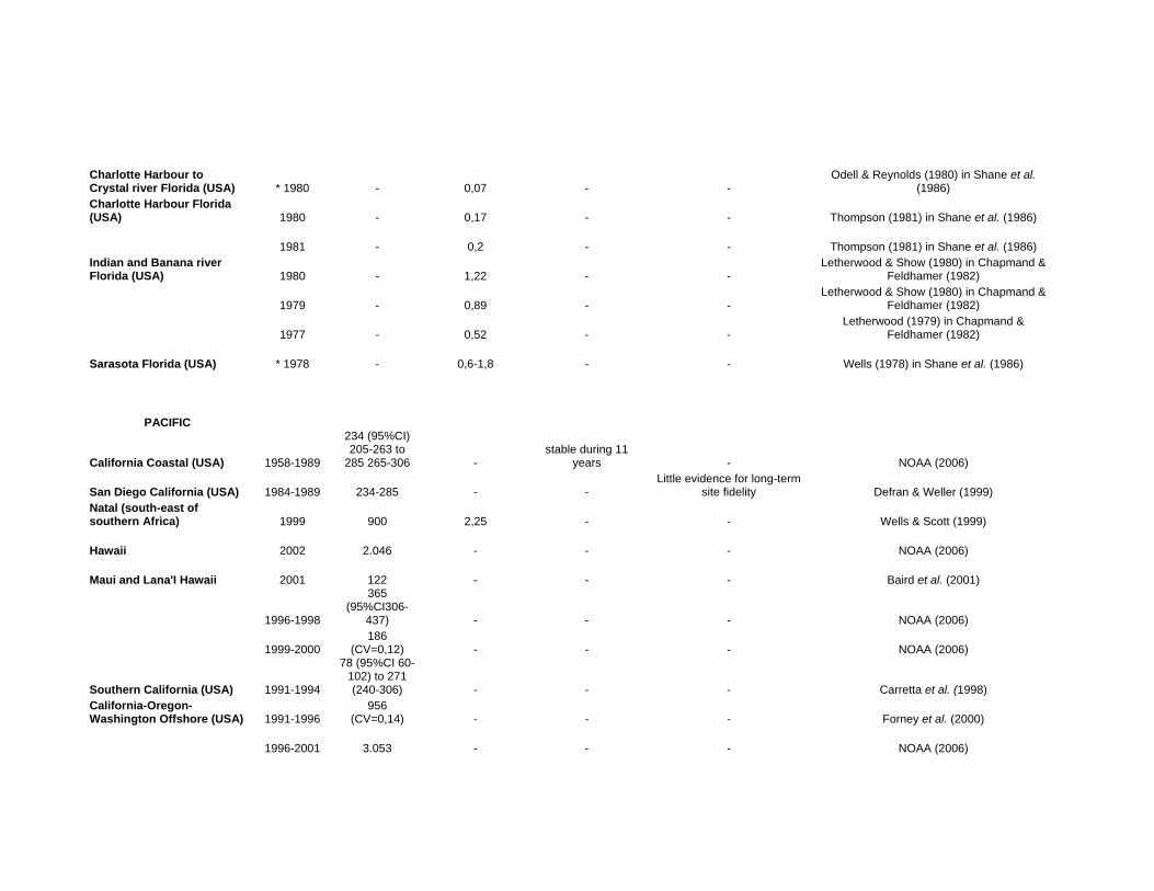
Charlotte Harbour to Crystal river Florida (USA) * 1980 - 0,07 - -
Odell & Reynolds (1980) in Shane et al. (1986)
Charlotte Harbour Florida (USA) 1980 - 0,17 - - Thompson (1981) in Shane et al. (1986)
1981 - 0,2 - - Thompson (1981) in Shane et al. (1986) Indian and Banana river Florida (USA) 1980 - 1,22 - -
Letherwood & Show (1980) in Chapmand & Feldhamer (1982)
1979 - 0,89 - - Letherwood & Show (1980) in Chapmand &
Feldhamer (1982)
1977 - 0,52 - - Letherwood (1979) in Chapmand &
Feldhamer (1982)
Sarasota Florida (USA) * 1978 - 0,6-1,8 - - Wells (1978) in Shane et al. (1986)
PACIFIC
California Coastal (USA) 1958-1989
234 (95%CI) 205-263 to
285 265-306 - stable during 11
years - NOAA (2006)
San Diego California (USA) 1984-1989 234-285 - - Little evidence for long-term
site fidelity Defran & Weller (1999) Natal (south-east of southern Africa) 1999 900 2,25 - - Wells & Scott (1999)
Hawaii 2002 2.046 - - - NOAA (2006)
Maui and Lana'I Hawaii 2001 122 - - - Baird et al. (2001)
1996-1998
365 (95%CI306-
437) - - - NOAA (2006)
1999-2000 186
(CV=0,12) - - - NOAA (2006)
Southern California (USA) 1991-1994
78 (95%CI 60-102) to 271 (240-306) - - - Carretta et al. (1998)
California-Oregon-Washington Offshore (USA) 1991-1996
956 (CV=0,14) - - - Forney et al. (2000)
1996-2001 3.053 - - - NOAA (2006)

Amakusa western Kyushu, Japan 1995-1997
218 (CV=5,41%) - - - Shirakihara et al. (2002)
MEDITERRANEAN
Alboran sea (Spain) 2000-2003 584 95%CI
278-744 0,04 Decreasing - Cañadas & Hammond (in press) in Reeves
& di Sciara (2006)
Almeria (Spain) 2001-2003 279 95%CI
146-461 0,06 Decreasing - Cañadas & Hammond (in press) in Reeves
& di Sciara (2006) Asinara island National Park (Italy) 2001
22 95%CI 22-27 0,05 Decreasing -
Lauriano et al. (2003) in Reeves & di Sciara (2006)
Balearic Islands & Catalonia (Spain) 2002
7.654 95%CI 1.608-15.766 0,08 Decreasing -
Forcada et al. (2004) in Reeves & di Sciara (2006)
Balearic Islands (Spain) 2002 1.030 95%CI
415-1.849 0,08 Decreasing - Forcada et al. (2004) in Reeves & di Sciara
(2006)
Gulf of Vera (Spain) 2003-2005 256 95%CI
188-592 0,04 Decreasing - Cañadas (unpublished) in Reeves & di
Sciara (2006)
Valencia (Spain) 2001-2003 1.333 95%CI
739-2.407 0,04 Decreasing - Gomez de Segura et al. (in press) in
Reeves & di Sciara (2006) North Adriatic Sea (Gulf of Trieste, Slovenia) 2002-2004 47 0,08
Decline 50% the past 50 years - Bearzi et al. (2004)
Strait of Gibraltar 2005 258 95%CI
226-316 0,51 - - de Stephanis et al. (2005) in Reeves & di
Sciara (2006)
Amvrakikos Gulf (Greece) 2001-2005 152 95%CI
136-186 0,38 - - Reeves & di Sciara (2006) North-eastern Adriatic sea (Kvarneric, Croatia) 1990-2004 120 -
Decline 50% the past 50 years - Reeves & di Sciara (2006)
Alboran sea and Murcia (Spain) 2004-2005 - 0,07 Decreasing -
Cañadas (unpublished) in Reeves & di Sciara (2006)
Lampedusa island (Italy) 1996-2000 140 - - - Reeves & di Sciara (2006)
Ionian Sea (Greece) 1993-2003 48 - - - Reeves & di Sciara (2006) Central Adriatic Sea (Kornati & Murtar sea, Croatia) 2002 14 - - - Reeves & di Sciara (2006)
Tunisian waters 2001-2003 - 0,19 - - Ben Naceur et al. (2004) in Reeves & di
Sciara (2006)

BLACK SEA
Declining until 1983. increasing
1993-2005, declining 2006 Reeves & di Sciara (2006)
Turkish Straits System (Bosphorus, Marmara Sea and Dardanelles) 1997
495 95%CI 203-1,197 - -
Dede (1999), cited after: IWC (2004) in Reeves & di Sciara (2006)
1998 468 95%CI 184-1,186 - -
Dede (1999), cited after: IWC (2004) in Reeves & di Sciara (2006)
Kerch Strait 2001 76 95%CI 30-
192 - - Birkun et al. (2002) in Reeves & di Sciara
(2006)
2002 88 95%CI 31-
243 - -
Birkun et al. (2003) in Reeves & di Sciara (2006)
2003 127 95%CI
67-238 - - Birkun et al. (2004) in Reeves & di Sciara
(2006) NE shelf area of the Black Sea 2002
823 95%CI 329-2,057 - -
Birkun et al. (2003) in Reeves & di Sciara (2006)
NW, N and NE Black Sea within Ukrainian and Russian waters 2003
4.193 95%CI 2.527-6.956 - -
Birkun et al. (2004) in Reeves & di Sciara (2006)

2.2. Studied Area Cardigan Bay is located in West Wales, UK (Figure 3). Cardigan Bay Special
Area of Conservation (SAC) is situated off south Ceredigion and north
Pembrokeshire in the southern part of Cardigan Bay. The landward boundary
runs along the coast, from Aberarth to just south of the Teifi Estuary at the
following coordinates (expressed as decimal degrees): South Lat: 52.0783
Long: 4.7650, West Lat: 52. 2186 Long: 5.0042, North Lat: 52.4300 Long:
4.3967, East Lat: 52.2500 Long: 4.2333 (Baines, et al., 2002; Figure 3). The
site extends approximately twelve miles offshore, with an area of 1039 km2
subdivided in 517 km2 inshore and 522 km2 offshore.
Cardigan Bay’s topography is characterized by high cliffs, small coves and a
few larger sandy beaches. The Teifi is by far the largest river to flow into the
bay. The middle and northern sections of the Cardigan Bay coast have
generally a low-lying topography while the north-western part of the Bay is
cliff-bound and rugged, with small coves and offshore islands. The Bay is a
shallow basin comprising a mixture of sediments which tend to grade from
gravel and cobbles offshore to a finer sand and silt nearshore, although
patches of cobble and boulder occur all along the coast. The distribution of
sea bed sediments is largely dependent upon tidal current strength; gravels
occur where the currents are strongest, and muds where they are weakest
(Baines, et al., 2000). The water depth in the bay does not exceed 50m and
becomes increasingly shallow from west to east, with an average depth of
approximately 40m (Evans, 1995).

Figure 3: Cardigan Bay (SAC) in UK.

Cardigan Bay and the Irish Sea are important marine areas. Warm waters
from the North Atlantic Drift meet cooler, tidally driven waters at both the
northern and southern ends of the Irish Sea. This produces nutrient upwelling
that provide suitable conditions for plankton concentrations to develop, and
upon which abundant fish, seabirds, seals and cetaceans feed. The waters
are often relatively calm, being protected from the Atlantic by the country of
Ireland (Evans, 1995).
2.3. Photo-identification (Photo-ID) To study the distribution, abundance and dynamics of an animal population, it
is essential to be able to recognise and follow individuals within a population
through time. Cetaceans are only visible for a brief moment, which makes the
study of these animals quite complicated. With the development of photo-ID
techniques, scientists are able to do this without unduly disturbing the
animals.
The photo-ID technique consists of the identification of individuals using
photographs of natural markings. Recognition of individual bottlenose
dolphins is based almost entirely on the shape of the dorsal fin, scars that are
permanent marks, (e.g. missing pieces from the trailing edges of the dorsal
fins or nicks), pigmented areas, and a range of scratches and skin bruises
(Figure 4). This technique was first used in bottlenose dolphin identification in
the 1970’s (Würsig & Würsig, 1977).
Figure 4: First photo showing nicks. Second photo showing pigmented area. Third photo showing scratches and skin bruises.

The method of photo-identification is based on the assumptions that the
species are correctly identified. In mark-recapture studies, the two main types
of mistakes are called false positives and false negatives. False positives
occur when two photos of two different individuals are erroneously matched
as the same individual, leading to underestimation errors in population
estimates, especially for large populations of less easily identifiable species.
False negatives happen when two sightings of the same individual do not get
matched and are marked as different individuals (Gunnlaugsson &
Sigurjónsson, 1990; Stevick, et al., 2001), and therefore, overestimate the
population size. Errors can be caused by poor quality photographs, less than
ideal observation conditions, and the heterogeneity of samples due to the lack
of distinctiveness or permanence of the markings (Stevick, et al., 2001).
Heterogeneity of samples and distinctiveness of marks can have serious
effects on population abundance estimations. Wells & Scott (1990) used two
mark-recapture techniques to estimate population size of bottlenose dolphins
in Florida, and found that both Petersen (also called the Lincoln index) and
Schnabel methods underestimated the known population size, but that the
Schnabel method was less biased. They argued that the bias was probably
caused by the heterogeneity of sightings, as varying ages and sex condition
were shown to have different sightings probabilities.
However, not all these errors can be eliminated, and the resulting decrease in
sample size will adversely affect the precision of the population abundance
estimate (Stevick, et al., 2001).
2.4. Mark Recapture Mark recapture studies are a powerful tool for conservation managers, and
can be used in any situation where animals can be marked (or otherwise
identified) and detected later by capture or sighting. An important distinction

can be made between open and closed populations in mark recapture
studies. A closed population remains constant in size and composition during
the study, while an open population is subject to animal births, deaths, or
migrations. Although all populations are subject to these processes, it is
possible effectively to have closure by doing the study over a short time, and
this is often desired. In order to apply closed population models with
confidence, the following assumptions need to be fulfilled:
(i) a marked animal will be recognized if recaptured
(ii) marked animals have the same probability of being recaptured as
unmarked animals,
(iii) marks are not lost,
(iv) within a sample, all the individuals have the same probability of
being captured
(Hammond, P.S. 1990; Campbell et al., 2002; Shirakihara et al., 2002;
Chilvers & Corkeron, 2003; Irwin & Würsig, 2004).

3. PROBLEM and JUSTIFICATION
3.1. Problem The current status of Cardigan Bay bottlenose dolphin population does not
have yet to be fully assessed, nor has it been evaluated how Cardigan Bay
bottlenose dolphin population size has responded to the conservation
strategies and an implemented management plan.
3.2. Justification Cardigan Bay is one of the very few areas around the UK, as Moray Firth,
where significant numbers of bottlenose dolphin are known to occur regularly
(Ceredigion County Council et al., 2001). This is why the bottlenose dolphin
Cardigan Bay population has been protected since 2001 with conservation
strategies and a management plan implemented after its proposal as a
Special Area of Conservation (SAC). The management plan indicated two
important attributes to be monitored in the bottlenose dolphins: annual
abundance (Taylor & Gerrodette, 1993), and spatial distribution within the
SAC (Ceredigion County Council et al., 2003). It was not until 2004 that this
area was formally designated an SAC under the European Union’s Habitats
Directive parameters, in order to maintain the bottlenose dolphin population at
favorable conservation status.

4. AIMS
4.1. General Aim To observe the trend in the bottlenose dolphin population size in Cardigan
Bay (SAC).
4.2. Specific Aims
• To estimate the population size during a period of three years 2003,
2004 and 2005.
• To compare the population size obtained in this period (2003 to 2005)
with information collected in the past, in order to establish a trend.

5. MATERIALS and METHODS
5.1. Survey Design 5.1.1. Survey Population
The survey population was that of the Cardigan Bay (SAC) bottlenose dolphin
(Tursiops truncatus).
5.1.2. Survey Variables
The independent variable was time, and the dependent variables were
population size and trend.
5.2 Method This study comprised a combination of data obtained by the use of line-
transect and Photo-ID methodology (photos were analyzed using Adobe
Photoshop software and Fax Viewer) and the mark-recapture method. With
the mark-recapture method, the first time an individual is sighted in the year of
survey, it is marked, and every time it is sighted again, it is considered as
recaptured. To meet assumptions of the mark-recapture method (mentioned
above), the following parameters were considered: For assumption one, out
of focus, or poor quality photographs were discarded, and the identification
was confirmed by a second observer. The second assumption is met because
photo-ID does not involve physical interaction (Wilson et al., 1999). The third
assumption is easily met because permanent marks were used, but the fourth
assumption can be violated if it is assumed that all the animals behave in the
same way. Since individual differences in surfacing rate and boat avoidance
behaviour affect the probability of obtaining a usable photograph (Hammond,
1986; termed heterogeneity of capture probability), it was necessary to use a
model that can relax this assumption; otherwise it would result in an
underestimation of population size.

Since allow heterogeneity of capture probabilities and this is problematic in
open population models, close model were use (Wilson et al., 1999).
Population closure is only a reasonable assumption when experiments are of
relatively short duration. The data were analyzed through CAPTURE
application of program MARK v.4.1 (Mark and Recapture Survival Rate
Estimation), developed by the Department of Fisheries and Wildlife, Colorado
State University (2004). This application has 11 available models that test for
three sources of variation in sightings probabilities; that of (i) the
heterogeneity response (Mh), assumes that each animal has its own unique
capture probability, which remains constant over all the sampling times (ii) the
trap response or behavioural response (Mb), where the animal may become
either ‘trap happy’ or ‘trap shy’ after their first capture and (iii) the time
variation or Schnabel Model (Mt), assumes that every animal in the population
has the same probability of capture at each sampling time. The 11 models
were all based on these principles and/or combinations of the three (for
example, Mbh, Mth, Mtb), plus one additional model where probability of
capture remains constant (M0).
In this study, the models used were selected purely on biological grounds.
The time heterogeneity model (Mth) (Chao et al. 1992), in which the
assumptions of heterogeneity and time were relaxed, was applied. Chao et al.
(1999) have derived a nonparametric estimator for abundance for the model
(Mth) using the idea of sample coverage (defined as the relative fraction of the
total individual capture probabilities of the capture animals) and an expression
for its asymptotic variance from an expanded Taylor series (Wilson et al.,
1999).
Conversely, however, both the null model (M0) and the behavioural models
(Mb) were largely ignored, the reasons being that the null model is unlikely to
occur under natural circumstances, and as photo-identification uses existing
marks, it involves no physical interaction between the animals and the

researcher in relation to the marking event, and so behavioural responses of
this type cannot occur, so the behavioural models were simply not applicable
to the study (Wilson et al., 1999).
5.3. Data Collection Data were collected during boat surveys within Cardigan Bay SAC during
2003, 2004 and 2005, as part of Sea Watch Foundation’s research on
bottlenose dolphins. The surveys were conducted either aboard the MV
Sulaire, that is a 10m charter vessel, or, in 2005, the MV Dunbar Castle. MV
Sulaire was equipped with a Global Positioning System (GPS), a Shipmate
RS 5700, as well as a semi-displacement hull and 380hp turbo diesel engine.
The observational platform was 3m above sea level having a viewing angle of
360°, although observers mainly concentrated on 180° from each side and
ahead of the boat. The surveys were carried out between April and
November, which were months with best weather, light, wind and sea
conditions, in Beaufort sea state of 0 - 3 during good light conditions, to make
the sightings more reliable (Barco, et al., 1999). When the sighting conditions
were good, i.e. sea state 2 or less, low swell, and no precipitation or fog, the
photo-identification surveys were combined with distance-sampling surveys
for bottlenose dolphins, harbour porpoise (Phocoena phocoena) and Atlantic
grey seals (Halichoerus grypus). The boat surveys were conducted following
predefined transect routes to cover the area uniformly (Figure 5). Each
transect was conducted at a speed of 8 knots (14 km per hour). Since this is
twice the average travel speed of dolphins, it reduces the probability of
meeting the same individuals, and thus them being counted more than once.

Figure 5: Predefined transects in Cardigan Bay SAC.
A Sightings Form (Annex 2) was also completed to log bottlenose dolphin
reactions to the boat, dolphin behaviour, all recorded GPS positions, and both
distance and angle estimates. The time and the location were recorded once
dolphins were sighted. To be photographed, the vessel may need to
approach the dolphins, whereupon the transect was abandoned. An
encounter was defined as the period spent photographing a dolphin group.
During encounter time, pictures were taken with a Canon D60 digital camera
with 75-300mm zoom lens (f 4.0 – 5.6). The main objective of each encounter
was to take the highest possible number of clear images from both sides of
each individual. So in an Encounter Sheet (Annex 3), encounter length and
number of encounters, and a log of picture frames taken were all recorded. A
spacer picture was taken at the start and end of each encounter.

Encounters were continued until all the members of the group had been
photographed or the contact had been lost. If signs of avoidance were shown,
or after approximately ten minutes without a sighting, the survey leader had to
decide whether to go back for tracking or continuing the line transect survey
using Distance.
5.4. Data Analysis 5.4.1. Individual Recognition from Identification Pictures.
Fin morphologies of individuals were identified from photographs of their
dorsal fin. Markings that occur naturally, like skin pigmentation, fin notches,
tears, deformities, tooth rakes and skin bruises on their dorsal fin and flanks,
were examined with emphasis on marks that persist throughout the study
period. The majority of the features were used to confirm matches, reducing
the possibility of false positives (Scott, et al., 1990; Würsig, & Jefferson,
1990). Using a light box and 8x magnifier glass, transparencies were
analyzed whilst downloaded digital pictures were examined using Adobe
Photoshop software and Fax Viewer.
A Film Sheet (Annex 4) was completed for the slides, and an Excel
spreadsheet for the digital pictures. For each picture a quality grade (scored
1-4), was assigned, based on image size, focus, lighting, angle of fin and
exposure. For example, a photograph that had the subject full frame, in sharp
focus and at a good angle was recorded as 1, whereas, a photograph in
which only a part of the fin was visible was recorded as 4. Photographs with
insufficient data or of poor quality were discarded.
Each match was identified and then subjected to a similar independent
analysis by a second observer, thus avoiding bias and reducing the possibility
of identifying false positives and false negatives. Profiles for both right and left
flanks of each animal were selected from the best images to be catalogued.
Finally, an encounter number was assigned, where a unique number was
given to each new studied animal.

5.4.2. Data Analysis for Population Size
Using the FORTRAN program MARK v.4.1, population estimates were made,
based on the number of marked individuals. In order to analyze the encounter
histories for the marked animals selected in this program, data were
transcribed into binary form, where the number ‘1’ indicated that an animal
had been sighted, and ‘0’ indicated that the animal had not been sighted.
The total population size was estimated from the proportion of marked
animals. The proportion of marked animals in each encounter was calculated
by taking the number of dolphins seen, and subsequently counting the
number of marked animals present in the encounter. The proportion of
marked dolphins per year was calculated as the average for all encounters.
For each surveyed year, the marked individual proportion was 0.71 in 2003,
0.62 in 2004 and 0.51 in 2005. The population estimates derived by MARK of
Mth model were recalculated and adjusted with the proportion of unmarked
individuals using the following equation (Wilson et al., 1999):
θ̂
ˆˆ NNTotal =
where TotalN̂ = total population size, N̂ = mark-recapture estimates of
population size, and θ̂ = proportion of animals with marks in the population.
A Kruskal-Wallis test was used to test for significant differences in population
size between the three years of study. To make this calculation, a total of
three values of population size were obtained per year, calculating the
population size in the three main months of the years (July, August and
September); a Kruskal-Wallis test was applied comparing the months, so as
to be sure that no effect of time existed in the population size estimate.
A population trend was more difficult to calculate, due to the short time of
study (three years), given that Wilson et al. (1999), found that more than eight
years data collection was needed to detect a significant (at the 10%
probability level) trend in population size, given that dolphins are long-lived
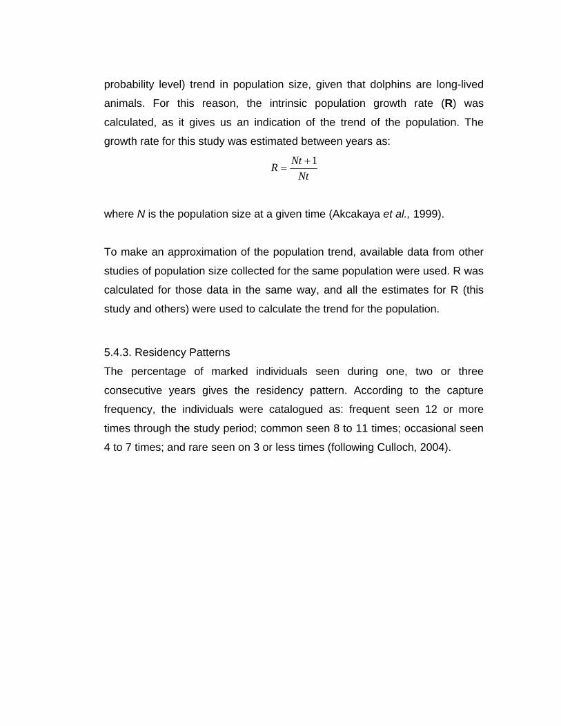
animals. For this reason, the intrinsic population growth rate (R) was
calculated, as it gives us an indication of the trend of the population. The
growth rate for this study was estimated between years as:
NtNtR 1+
=
where N is the population size at a given time (Akcakaya et al., 1999).
To make an approximation of the population trend, available data from other
studies of population size collected for the same population were used. R was
calculated for those data in the same way, and all the estimates for R (this
study and others) were used to calculate the trend for the population.
5.4.3. Residency Patterns
The percentage of marked individuals seen during one, two or three
consecutive years gives the residency pattern. According to the capture
frequency, the individuals were catalogued as: frequent seen 12 or more
times through the study period; common seen 8 to 11 times; occasional seen
4 to 7 times; and rare seen on 3 or less times (following Culloch, 2004).

6. RESULTS and DISCUSSION
6.1. Results
The survey effort decreased with survey time, due to logistic conditions, and
the encounters decreased proportionally with number of survey days (Table
2).
A total of 46 transect legs were covered in 2003 (507 Km), 48 legs in 2004
(653 km) and 92 transect legs in 2005 (1490) of a total of 30 transect legs.
Table 2: Effort survey. The months of each year were the survey period for the line transect method. The number of days and trips made each year, number of hours dedicated to the survey, number of encounters, number of hours spent in encounters, and surveyed distance are observed in the columns.
Year Months Survey Days Survey Trips S. Hour Effort Encounters Ecou. Hours Distance
2003 May-Sept 74 74 328 139 17.05 507 Km
2004 May-Sept 59 59 263 121 26.3 653 Km
2005 April-Nov 33 33 209 66 21.11 1490 Km
TOTAL 166 166 800 326 64.46 2650 Km
A total of 121 different individuals were photographer (well marked plus
individuals photographed just in the right side of the fin) in 2003; 108 in 2004
and 154 in 2005.
The mark-recapture analysis suggested an average population size of 178 +/-
22 individuals. The results showed an increasing tendency in the intrinsic
population growth rate (R) between years (Table 3). Nevertheless no
significant differences were found in the population size estimates through
years (Kruskal-Wallis test, H2, N=3 = 2.0; p = 0.36, Figure 6); and no effect of
time in the population size estimate was found (Kruskal-Wallis test, p = 0.22).

Table 3: Estimation of population size, using Chao (Mth) model, where N̂ is the population
size using marked animals, θ̂ is the proportion of marked animals, TotalN̂ is the total
population size, SE is the standard error of the N̂ population, CI are the confidence intervals
of N̂ population, P is the capture probability, and R is the intrinsic population growth between two consecutive years.
Three years is not enough time to see a trend in the population size for a
long-lived animal like the bottlenose dolphin and cetaceans in general. A
growing population tendency of 46.4% was observed in 16 years (1989 to
2005) when analyzing data collected from different studies, but this is a
dangerous comparison since the estimates pre-2000 involved very different
spatial coverage and levels of effort. And the realistic comparison can be
made since 2001.

Figure 6: Kruskal-Wallis results for the comparison between years.
The full set of results obtained by the program MARK for the population
estimations of the marked animals, for each year using Chao time-
heterogeneity dependency model (Mth); are shown in annex 5.
The discovery curve (Figure 7) has yet to reach an asymptote.

Figure 7: Discovery curve of cumulative number of individuals identified throughout number of encounters.
Photo identification and distance sampling are both commonly used
techniques to monitor marine mammal populations, but rarely are both used
on the same population, the two techniques could be used in synchrony on
bottlenose dolphins, using abundance estimates derived from distance
sampling and photo ID (Felce et. al., 2006), the following abundance
estimates were obtained in 2005 (Figure 8):
• 150 (80-280) using Distance 4.1
• 227 using Mark Recapture
• 175 based on the average proportion of well-marked
individuals.

Figure 8: Abundance estimates derived between 2003 and 2005, using different techniques, Distance, Mark-recapture (photo ID), and based on the average proportion of well-marked individuals.
This population showed a high residency pattern, since 71% of the marked
individuals were seen in two or three consecutive years (Figure 9). 51
individuals (the 42.1% of the total marked individuals recorded) were
catalogued as frequent and common, while 31 dolphins (25.6%) were
occasional, and 39 individuals (32.2%) were rare (Figure 10). A high capture
frequency (representing the times that one animal was seen during the study
period), was obtained, ranging from 1 to 33 times. This confirmed the high
site fidelity within the population.

Figure 9: Percentage of marked animals seen during one year (28%), two years (40%) and three consecutive years (31%).
Figure 10: Histogram showing the distribution of recapture frequencies for all marked bottlenoses identified in the present study during 2003 to 2005.

6.2. Discussion
The Cardigan Bay bottlenose dolphin population seems to be small when
compared with the size of other coastal and offshore populations recorded
(Table 1), but for the area of study it is one of the larger ones in North West
Europe (Evans personal communication, 2006). Habitats in shallow waters
and protected from open oceans; as is the case for Cardigan Bay, may attract
small populations of bottlenose dolphin (Wells et al., 1997). However, the
Cardigan Bay population was higher than some other critically smaller coastal
populations, which did not reach the 100 individuals, such as those at Moray
Firth (Scotland), Western Galveston Bay (US), Asinara Island National Park
(Italy), Central Adriatic Sea (Kornati & Murtar Sea, Croatia), North Adriatic
Sea (Gulf of Trieste, Slovenia), Ionian Sea (Greece), and Kerch Strait (Table
1). According to some population viability analyses of bottlenose dolphins,
populations of less than 100 individuals will face high extinction probabilities
(Thompson et al., 2000).The average Cardigan Bay population size in the
three years of study (178 individuals) was 7% higher than that of other
coastal populations (166, Table 1). However, it is much smaller than oceanic
populations, which can reach the 9.912 individuals (Eastern Gulf of Mexico,
Table 1). However, population size is a parameter very hard to compare
directly in space and time, due to the range in size of sampling area surveyed
in different studies. For this reason, we consider density as a better source of
comparison between populations. The density value found in Cardigan Bay
(0.18 indivs/ km2) was low when compared with the average density of 0.51
indivs/ km2 registered in other areas (Table 1). When compared with density
values for coastal areas (with an average of 0.22 indivs/ km2), Cardigan Bay
population density was 18% lower. Nevertheless, there are places with even
lower bottlenose dolphin density registered, such as the Alboran Sea, Gulf of
Vera, and Valencia in the Mediterranean Sea, with 0.04 indivs/ km2 (Table 1),
in contrast to Aransas Pass, Texas in the North-West Atlantic, with the
highest density values registered (4.8 indivs/ km2; Table 1). Cardigan Bay

presented a population abundance estimate slightly higher than the average,
but with a lower density, compared with other studies.
According to our results and comparisons, while the Cardigan Bay bottlenose
dolphin population seems to be stable in the short term (three years), a
tendency for a growing population seems to be the pattern. The size of this
population was 125 individuals in 1993, a number that is generally
acknowledged by Ceredigion Country Council et al., (2001) to be small and
vulnerable to impacts, reducing the ability to sustain itself. However, in 2005
we obtained an abundance estimate of 227 individuals, a number rather
higher than the one obtained in the 2001 (Baines et al, 2002), who observed
a total of 215 individuals (Table 1), supporting this hypothesis of recent
population growth.
Considering that Cardigan Bay’s bottlenose dolphin population growth rate
was 46.4% in a period of 16 years (2.9% per year), we can assume under
similar conditions that the Cardigan bottlenose dolphin population could
double in size in 34 years. This value is just the 13% lower than which Perrin
& Reilly, (1984), Slooten & Lad, (1991), and Hare et al., (2002) suggested as
the doubling time for a dolphin population (39 years). However, more
information would be necessary to verify this population trend, the good
source of resources provided by the Bay, as well as its carrying capacity to
support a growing population of bottlenose dolphin.
The population growth rate depends on births, deaths, and migration rates.
Although there is insufficient information to identify which factor is most
influencing the Cardigan Bay population, we consider that a good proportion
of population growth is due to the increasing birth rate; since a significant
number of calves were observed during the study (29.1% of the encounters
had calves with an average of 1.39 calves per encounter). Additionally, the
proportion of individuals seen only during a single year of sampling (28%,
Figure 3) suggested some immigration. Some of the factors that have
probably allowed the increase in the dolphin population in this Bay may be a

consequence of an appropriate effort to conserve the population, and to a
decrease in mortality rates. Conservation strategies have been applied in the
management plan of the SAC since 2001, which include: 1) a management
control of any negative impacts on the dolphins as a result of changes in
natural variables (salinity, sea temperature, fronts etc) influenced by humans
activities, and 2) consideration of any land influences such as run-off, which
carry polluted sediments and might have a negative effect on dolphin health
and distribution (see Cardigan Bay Management Plan; Ceredigion Country
Council et al., 2001 for more details). Since disturbances cause fluctuation in
population size (Akcakaya, 1999), future research needs to evaluate to what
degree conservation strategies minimize human disturbance and may result
in an increase in dolphin reproductive success and/or survival rate, and thus
in population size.
The apparent success of bottlenose dolphins at Cardigan Bay contrasts with
failures to increase the population size of marine mammals in other protected
marine areas, which have aimed to protect different species. For example,
dugong (Dugong dugon) populations of Nigaloo and Sark Bay Marine Parks
in Australia are declining despite efforts to protect them. Preen (1998)
suggests that these results can be explained by the low level of protection
provided by some Marine Protected Areas (MPAs) where harmful activities,
such as commercial fishing, seismic surveys, and oil and gas drilling, are
permitted. This shows the importance of full conservation strategies where
the population to conserve should be the priority, and all activities must be
evaluated based on the impacts to these populations.
Another issue in current conservation strategies is the size of protected areas;
since larger areas are needed for reserves to achieve benefits (Gerber et al.,
2003) such as a higher carrying capacity for dolphins and other populations.
Most reserves are too small, representing only a small portion of the total

range of species (Gell & Roberts, 2003), as in Tursiops truncatus. Cardigan
Bay represents what is believed to be their main activity area in Wales
(Ceredigion County Council et al., 2001). This may be related according to
Shane et al., (1986) to a protected geographical area, predator absence,
good food resources, and a low level of disturbance. As a consequence of
these factors, the Cardigan Bay population shows high site fidelity.
Comparing these results with the results obtained by Culloch (2004) for the
Moray Firth, and having in mind that the Moray Firth population is considered
a population with high site fidelity (Culloch, 2004 and Wilson et al., 1999) the
high site fidelity for Cardigan Bay population is confirmed, since 42.1% of the
marked individuals were catalogued as frequent and common in Cardigan
Bay and just 28.9% on the south side of the Moray Firth; 32.2% were rare in
Cardigan Bay and 43.4% in the Moray Firth. Cardigan Bay fulfills all the
characteristics of a population with site fidelity, which may contribute to the
stability of this population in the Bay.
7. CONCLUSIONS
• No significant differences in the population size results were found
between the three years of study.
• A growing tendency in the population size was found over a period of 5
years.
• High site fidelity of a portion of the dolphin population was found in
Cardigan Bay.
• A longer time series data set is needed for more accurate results and
understanding of the population.
8. RECOMMENDATIONS
It is important to carry out a monitoring program and collect accurate time
series data of the population status. This study followed the methodology
proposed by Baines et al., (2002) which allowed temporal comparisons,
covering the total Special Area of Conservation and using a simple
confidence model for the characteristics of the population. In the long-term,
an extension of this study will give more reliable results. This is why this
methodology has been recommended for future research. It would be useful
to address variables such as birth and death rates, migration rates, and
trends in these vital parameters; to have a complete understanding of the
population dynamics of dolphins in Cardigan Bay. A good comprehension of
the ecosystem is also fundamental, as well as of resource availability to
evaluate the ecosystem’s carrying capacity, and up to what point the growth
of the population is healthy and sustainable. Combine mark-recapture studies
with line-transect surveys since they are providing complementary
information.
It is recommended that conservation strategies are continued in order to
maintain the population at favorable conservation status, and because the
bottlenose dolphin population seems to be responding in a positive way to
them.
Since little is known about the winter range of the Cardigan Bay dolphin
population, it is important to address this issue to give the population
complete protection over its full range, and if necessary, to consider the
proposal of marine reserve networks.

9. REFERENCES
ACCOBAMS. 2004. Conservation Status of Bottlenose Dolphin (Tursiops
truncatus): Assessment Using Morphological and Genetic Variation.
Report to ACCOBAMS scientific committee. Second Meeting of Parties
Palma de Mallorca.
Akcakaya, H.R., Burgman, M.A., & Ginzburg, L. 1999. Applied Population
Biology, principles and computers exercises using Ramas EcoLab 2.0.
Second Edition. Sunderland, Massachusetts: Sinauer Associates.
Arnold, H., Bartels, B., Wilson, B., & Thompson, P. 1997. The Bottlenose
dolphins of Cardigan Bay: Selected biographies of individual Bottlenose
dolphin recorded in Cardigan Bay Wales. Report to Countryside Council
for Wales; CCW Science Report No 209.
Arnold, H. & Mayer, S.J. 1995. The ecology of bottlenose dolphins in
Cardigan Bay, Wales, UK. In: Baines, M.E., Evans, P.G.H., & Shepherd,
B. 2000. Bottlenose dolphins in Cardigan Bay, West Wales. Sea Watch
Foundation Report. pp. 29.
Baines, M.E., Evans, P.G.H., & Shepherd, B. 2000. Bottlenose dolphins in
Cardigan Bay, West Wales. Sea Watch Foundation Report. pp. 29.
Baines, M.E., Reichelt. M., Evans, P.G.H., & Shepherd, B. 2002. Bottlenose
dolphins studies in Cardigan Bay, West Wales. Final Report to
INTERREG. Sea Watch Foundation. pp 17.
Baird, R.W., Gorgone, A.M., Ligon, A.D., & Hooker, S.K. 2001. Mark-
recapture abundance estimate of bottlenose dolphins (Tursiops
truncatus) around Maui and Lana’I, Hawai’I, during the winter of
2000/2001. Report Prepared under Contact No 40JGNF0-00262 to the
Sothwest Fisheries Science Center National Marine Fisheries Service
8604 La Jolla Shores Drive La Jolla, CA 92037-1508 USA, 1-13.
Barco, S. G., Swingle, W. M., McLellan, W. A., Harris, R. N., & Pabst, D. A.
1999. Local abundance and distribution of bottlenose dolphins (Tursiops
truncatus) in the nearshore waters of Virginia Beach, Virginia. Marine
Mammal Science, 15(2):394-408.
Barham, E.G., Sweeney, J.C., Leatherwood, S., Beggs, R.K., & Barham, C.L.
1980. Aerial census of the bottlenose dolphin, Tursiops truncatus, in a
region of the Texas coast. In: Shane, S.H., Wells, R.S. & Würsig, B.
1986. Ecology, behavior and social organization of the bottlenose
dolphin: A review. Marine Mammal Science, 2(1):34-63.
Barros, N. B. & Odell, D. K. 1990. Food Habits of Bottlenose Dolphins in the
Southeastern United States. In: The Bottlenose Dolphin, S. Leatherwood
& R.R. Reeves, (eds.) Academic Press, San Diego. pp. 309-328.
Bearzi, G., Holcer, D., & di Sciara, G. 2004. The role of historical dolphin
takes and habitat degradation in shaping the present status of northern
Adriatic cetaceans. Aquatic Conservation: Marine and Freshwater
Ecosystems, 14: 363-379.
Bearzi, G., Politi, E., Agazzi, S., Bruno, S., Costa, M., & Bonizzoni, S. 2005
Occurrence and present status of coastal dolphins (Delphinus delphis
and Tursiops truncatus) in the eastern Ionia Sea. Aquatic Conservation:
Marine and Freshwater Ecosystems, 15: 243-257.
Ben Naceur L., Gannier A., Bradai M.N., Drouot V., Bourreau S., Laran S.,
Khalfallah N., Mrabet R., & Bdioui M. 2004. Recensement du grand
dauphin Tursiops truncatus dans les eaux tunisiennes. In: Reeves, R. &
di Sciara, N.G. (compilers and editors). 2006. The status and distribution
of cetaceans in the Black Sea and Mediterranean Sea. IUCN Centre for
Mediterranean Cooperation, Malaga, Spain. 137 pp.
Birkun A. Jr., Glazov D., Krivokhizhin S., & Mukhametov L. 2002. Distribution
and abundance of cetaceans in the Sea of Azov and Kerch Strait:
Results of aerial survey (July 2001). In: Reeves, R. & di Sciara, N.G.
(compilers and editors). 2006. The status and distribution of cetaceans
in the Black Sea and Mediterranean Sea. IUCN Centre for
Mediterranean Cooperation, Malaga, Spain. 137 pp.
Birkun A., Jr., Glazov D., Krivokhizhin S., Nazarenko E., & Mukhametov L.
2003. Species composition and abundance estimates of cetaceans in
the Kerch Strait and adjacent areas of the Black and Azov Seas: The
second series of aerial surveys (August 2002). In: Reeves, R. & di
Sciara, N.G. (compilers and editors). 2006. The status and distribution of
cetaceans in the Black Sea and Mediterranean Sea. IUCN Centre for
Mediterranean Cooperation, Malaga, Spain. 137 pp.
Birkun A.A., Jr., Krivokhizhin S.V., Glazov D.M., Shpak O.V., Zanin A.V., &
Mukhametov L.M. 2004. Abundance estimates of cetaceans in coastal
waters of the northern Black Sea: Results of boat surveys in August-
October 2003. In: Reeves, R. & di Sciara, N.G. (compilers and editors).
2006. The status and distribution of cetaceans in the Black Sea and
Mediterranean Sea. IUCN Centre for Mediterranean Cooperation,
Malaga, Spain. 137 pp.
Bristow, T. 1999. Activity and Behaviour of Bottlenose Dolphins (Tursiops
truncatus) in Cardigan Bay. MSc Thesis University of Wales, Bangor.
Ocean Sciences. pp.161.
Cañadas, A., & Hammond, P.S. In press. Model-based abundance estimates
for bottlenose dolphins off southern Spain: implications for conservation
and management. In: Reeves, R. & di Sciara, N.G. (compilers and
editors). 2006. The status and distribution of cetaceans in the Black Sea
and Mediterranean Sea. IUCN Centre for Mediterranean Cooperation,
Malaga, Spain. 137 pp.
Campbell, G. S., Bilgre, B. A., & Defran, R. H. 2002. Bottlenose dolphins
(Tursiops truncatus) in Turneffe Atoll, Belize: occurrence, site fidelity,
group size, and abundance. Aquatic Mammals, 28(2): 170-180.
Carreta, J.V., Forney, K.A., & Laake, J.L. 1998. Abundance of southern
California coastal bottlenose dolphins estimated from tandem aerial
surveys. Marine Mammal Science, 14(4): 655-675.
Ceredigion County Council, Countryside Council for Wales, Environment
Agency Wales, North Western and North Wales Sea Fisheries
Committee, Pembrokeshire Coast National Park authority,
Pembrokeshire County Council, South Wales Sea Fisheries Committee,
Trinity House & Dwr Cymru Welsh Water. 2001. Cardigan Bay Special
Area of Conservation Management Plan.
Ceredigion County Council, Countryside Council for Wales, Department of
Environment, Food and Rural Affairs, Department of Highways,
Properties and Works, Department of Trade and Industry, Environment
Agency Wales, Environmental Health Officer, National Assembly of
Wales, North Wales and North West Sea Fisheries Committee, Police
Against Wildlife Crime, Pembrokeshire County Council, Pembrokeshire
Coastal National Park Authority, Branch of Ministry of Defence,
Aberporth, South Wales Sea Fisheries Committee, Wildlife Safety at
Sea. 2003. Cardigan Bay Candidate Special Area of Conservation
Action Plan Review 1.
Chao, A., Lee, S.M., & Jeng, S.L. 1992. Estimating population size for
capture-recapture data when capture probabilities vary by time and
individual animal. Biometrics, 48: 201-216.
Chilvers, B.L., & Corkeron, P.J. 2003. Abundance of Indo-Pacific bottlenose
dolphins, Tursiops aduncus, off Point Lookout, Queensland, Australia.
Marine Mammal Science, 19(1): 85-95.
Culloch, R.M. 2004. Mark recapture Abundance Estimates and Distribution of
Bottlenose dolphins (Tursiops truncatus) Using the Southern Coastline
of the Outer Moray Firth, NE Scotland. MSc. Thesis. University of
Bangor, Wales. 39 pp.
Defran, R.H. & Weller, D.W. 1999. Occurrence and distribution, site fidelity,
and school size of bottlenose dolphins (Tursiops truncatus) off San
Diego, California. Marine Mammal Science, 15(2): 366-380.

Duffield, D.A., & Chamberlin-Lea, J. 1990. Use of Chromosome
Heteromorphisms in studies of Bottlenose Dolphin Population and
Paternities. In: The Bottlenose Dolphin, S. Leatherwood & R.R. Reeves,
(eds.) Academic Press, San Diego. pp. 609-620.
Evans, C.D.R. 1995. Offshore Environment. In: Coasts and Seas of the
United Kingdom, J. H. Barne, C. F. Robson, S. S. Kaznowska and J. P.
Doody, (eds.) Nature Conservation Committee, Peterborough. pp. 239.
Felce, T.H., Stone, E.B., Whiteford, J., James, E., Castrillon, J., & Evans,
P.G.H. 2006. To What Extent can distance Sampling be combined with
Photo Identification as a Monitoring Tool for Tursiops truncatus. Poster
European Cetacean Society conference Gdynia, Poland.
Fish, F.E., & Hui, C.A. 1991. Dolphin Swimming: A Review. Mammals
Review, 21(4): 181-195.
Forcada J., Gazo M., Aguilar A., Gonzalvo J., & Fernandez-Contreras M.
2004. Bottlenose dolphin abundance in the NW Mediterranean:
addressing heterogeneity in distribution. In: Reeves, R. & di Sciara, N.G.
(compilers and editors). 2006. The status and distribution of cetaceans
in the Black Sea and Mediterranean Sea. IUCN Centre for
Mediterranean Cooperation, Malaga, Spain. 137 pp.
Forney, K.A., Barlow, J., Muto, M.M., Lowry, M., Baker, J., Cameron, G.,
Mobley, J., Stinchcomb, C., & Carreta, J.V. 2000. U.S. Pacific Marine
Mammal Stock Assessments: 2000. NOAA-TM-NMFS-SWFSC-300.
Gailey, G.A. 2001. Computer systems for photo-identification and theodolite
tracking of cetaceans. MSc thesis, Texas A&M University, College
Station, TX. pp.125.
<http://www.tamug.tamu.edu/mmrp/GradStudents/Gailey/Gailey-
2001.pdf> [It consults: April 2006]
Gell, F.R., & Roberts, C.M. 2003. Benefits beyond boundaries: The fishery
effects of marine reserves. Trends in Ecology and Evolution, 18: 448–
455.

Gerber, L.R., Botsford, L.W., Hastings, A., Possingham, H.P., Gaines, S.D.,
Palumbi, S.R., & Andelman SJ. 2003. Population models for reserve
design: A retrospective and prospective synthesis. Ecological
Applications, 13: S47–S64.
Gomez de Segura A., Crespo E.A., Pedraza S.N., Hammond P.S., & Raga
J.A. In press. Abundance of small cetaceans in the waters of the central
Spanish Mediterranean. In: Reeves, R. & Notarbartolo di Sciara, G.
(compilers and editors). 2006. The status and distribution of cetaceans
in the Black Sea and Mediterranean Sea. IUCN Centre for
Mediterranean Cooperation, Malaga, Spain. 137 pp.
Gruber, J.A., 1981. Ecology of the Atlantic bottlenose dolphin (Tursiops
truncatus) in the Pass Cavallo area of Matagorda Bay, Texas. In: Shane,
S.H., Wells, R.S. & Würsig, B. 1986. Ecology, behavior and social
organization of the bottlenose dolphin: A review. Marine Mammal
Science, 2(1):34-63.
Gunnlaugsson, T., & Sigurjónsson, J. 1990. A Note on the problem of False
Positives in the Use of Natural Marking Data for Abundance Estimation,
In: Reports of the International Whaling Commission, Special Issue 12,
Hammond, P.S., Mizroch, S.A., & Donovan, G.P. (eds.) Cambridge
International Whaling Commission. pp. 143-145.
Hammond, P.S. 1986. Estimating the size of naturally marked whale
populations using capture–recapture techniques. Reports of
International Whaling Commission. Special Issue, 8:253-282.
Hammond, P.S. 1990. Heterogeneity in the Gulf of Maine? Estimating
humpback whale population size when capture probabilities are not
equal. Reports of the International Whaling Commission. Special Issue
12, 135–139.

Hansen, L.H. 1990. California Coastal Bottlenose Dolphins, In: The
Bottlenose Dolphin, S. Leatherwood & R.R. Reeves, (eds.) Academic
Press, San Diego. pp. 403-420.
Hare, M.P., Cipriano, F. & Palumbi, S.R. 2002. Genetic evidence on the
demography of speciation in allopatric dolphin species. Evolution, 56(4):
804-816.
Hubard, C.W., Maze-Foley, K., Mullin, K.D. & Schroeder, W.W. 2004.
Seasonal Abundance and Site Fidelity of bottlenose Dolphins (Tursiops
truncatus) in Mississippi Sound. Aquatic Mammals 30(2):299-310.
Irwin, L., & Würsig, B. 2004. A small resident community of bottlenose
dolphins, Tursiops truncatus, in Texas: Monitoring recommendations.
Gulf of Mexico Science, 1: 13-21.
IWC. 2004. Annex L. Report of the Sub-committee on Small Cetaceans. In:
Reeves, R. & Notarbartolo di Sciara, G. (compilers and editors). 2006.
The status and distribution of cetaceans in the Black Sea and
Mediterranean Sea. IUCN Centre for Mediterranean Cooperation,
Malaga, Spain. 137 pp.
Kerr, K.A., Defran, R.H., & Campbell, G. 2005. Bottlenose dolphins (Tursiops
truncatus) in the Drowned Cayes, Belize: Group size, site fidelity and
abundance. Caribbean Journal of Science, 41(1): 172-177.
Lauriano G., Mackelworth P., & Fortuna C.M. 2003. Densità e abbondanza
relativa del tursiope (Tursiops truncatus) nel parco nazionale
dell’Asinara, Sardegna. In: Reeves, R. & Notarbartolo di Sciara, G.
(compilers and editors). 2006. The status and distribution of cetaceans
in the Black Sea and Mediterranean Sea. IUCN Centre for
Mediterranean Cooperation, Malaga, Spain. 137 pp.
Leatherwood, S. 1979. Aerial survey of the bottlenose dolphins, Tursiops
truncatus, and the West Indian Manatee, Trichechus manatus, in the
Indian and Banana Rivers, Florida. In: Shane, S.H., Wells, R.S. &

Würsig, B. 1986. Ecology, behavior and social organization of the
bottlenose dolphin: A review. Marine Mammal Science, 2(1):34-63.
Leatherwood, J.S., Gilbert, J.W. & Chapman, D.G. 1978. An evaluation for
some techniques for aerial censuses of bottlenose dolphins. In: Shane,
S.H., Wells, R.S. & Würsig, B. 1986. Ecology, behavior and social
organization of the bottlenose dolphin: A review. Marine Mammal
Science, 2(1):34-63.
Leatherwood. S., & Show, I.T. 1980. Development of systematic procedure
for estimating size of “populations” of bottlenose dolphins. In: Chapman
& Feldhamer Wild Mammals of North America: Biology, Management,
and Economics. John Hopkins University Press, 1982. 369-414.
Leatherwood, J.S., & Reeves, R.R. 1982. Bottlenose dolphin (Tursiops
truncatus) and other toothed cetaceans. In: Shane, S.H., Wells, R.S. &
Würsig, B. 1986. Ecology, behavior and social organization of the
bottlenose dolphin: A review. Marine Mammal Science, 2(1):34-63.
Leatherwood, J.S., & Reeves, R.R. 1983. Abundance of bottlenose dolphins
in Corpus Christi Bay and coastal southern Texas. In: Shane, S.H.,
Wells, R.S. & Würsig, B. 1986. Ecology, behavior and social
organization of the bottlenose dolphin: A review. Marine Mammal
Science, 2(1):34-63.
Lewis, E.J. 1999. A digital database of photographically identified bottlenose
dolphins: Cardigan Bay, West Wales. In: Baines, M.E., Evans, P.G.H., &
Shepherd, B. 2000. Bottlenose dolphins in Cardigan Bay, West Wales.
Sea Watch Foundation Report. pp. 29.
Mitchell, E. (Ed). 1975. Report of the meeting on small cetaceans, Montreal,
April 1-11, 1974. In: Chapman & Feldhamer Wild Mammals of North
America: Biology, Management, and Economics. John Hopking
University Press. 1982. 369-414.
Mizroch, S.A., Beard, J.A., & Macgill, L. 1990. Computer Assisted Photo-
Identification of Humpback Whales. In: Reports of the International

Whaling Commission, Special Issue 12, Hammond, P.S., Mizroch, S.A.,
Donovan, G.P. (eds.) Cambridge: International Whaling Commission.
pp.63-70.
NOAA Fisheries (USA). Office of Protected Resources. Marine Mammal
Stock Assessment Reports (SARs) by Species/Stock.
<http://www.nmfs.noaa.gov/pr/sars/species.htm> [It consults: September
15, 2006].
Odell, D.K., & Reynolds, III. 1980. Abundance of the bottlenose dolphin,
Tursiops truncatus on the west coast of Florida. In: Shane, S.H., Wells,
R.S. & Würsig, B. 1986. Ecology, behavior and social organization of the
bottlenose dolphin: A review. Marine Mammal Science, 2(1):34-63.
Perrin, W.F., & Reilly, S.B. 1984. Reproductive parameters of dolphins and
small whales of the family Delphinidae. Pp. 97–133. In: Report of the
International Whaling Commission Special Issue 6.
Preen, A. 1998. Marine protected areas and dugong conservation along
Australia’s Indian Ocean coast. Environmental management, 22(2): 173-
181.
Read, A.J., Urian, K.W., Wilson, B., & Waples, D.M. 2003. Abundance of
bottlenose dolphins in the bays, sounds, and estuaries of North Carolina.
Marine Mammal Science, 19:59–73.
Reeves, R. & Notarbartolo di Sciara, G. (compilers and editors). 2006. The
status and distribution of cetaceans in the Black Sea and Mediterranean
Sea. IUCN Centre for Mediterranean Cooperation, Malaga, Spain. 137
pp.
Reeves, R.R., Stewart, B.S., Clapham, P.J., & Powell, J.A. 2002. Sea
Mammals of the World. First Edition. A & C Black. London.
Rice, D.W. 1998. Marine mammals of the world: systematics and distribution.
Society for Marine Mammalogy, Special Publication Number 4 (Wartzok
D, Ed.), Lawrence, KS. USA.

Schroeder, J. P. 1990. Breeding Bottlenose Dolphins in captivity. In: The
Bottlenose Dolphin, S. Leatherwood & R.R. Reeves, (eds.) Academic
Press, San Diego. pp. 435-446.
Scott, M.D., Wells, R.S., & Irvine, A.B. 1990. A Long-Term Study of
Bottlenose Dolphins on the West Coast of Florida, In: The Bottlenose
Dolphin, S. Leatherwood & R.R. Reeves, (eds.) Academic Press, San
Diego. pp. 235-244.
Shane, S.H. 1980. Occurrence, movements, and distribution of bottlenose
dolphins, Tursiops truncatus, in southern Texas. In: Shane, S.H., Wells,
R.S. & Würsig, B. 1986. Ecology, behavior and social organization of the
bottlenose dolphin: A review. Marine Mammal Science, 2(1):34-63.
Shane, S.H., Wells, R.S., & Würsig, B. 1986. Ecology behaviour and social
organization of bottlenose dolphin a review. Marine Mammal Science,
2(1):34-63.
Shirakihara, M., Shirakihara, K., Tomonaga, J., & Takatsuki, M. 2002. A
resident population of Indo-Pacific bottlenose dolphins (Tursiops
aduncus) in Amakusa, Western Kyushu, Japan. Marine Mammal
Science, 18(1): 30-41.
Slooten, E., & Lad, F. 1991. Population biology and conservation of Hector’s
dolphin. Canadian Journal of Zoology, 69:1701–1707.
Stensland, E., Carlen, I., & Sarnblad, A. 2006. Population size, distribution,
and behavior of Indo-Pacific bottlenose (Tursiops aduncus) and
humpback (Sousa chinensis) dolphins off the south coast of Zanzibar.
Marine Mammal Science, 22(3): 667-682.
de Stephanis R., Verborgh P., Pérez Gimeno N., Sánchez Cabanes A., Pérez
Jorge S., Esteban Pavo R., Séller N., Urquiola E., & Guinet C. 2005.
Impactos producidos por el tráfico marítimo en las poblaciones de
cetáceos en el estrecho de Gibraltar. Situación actual y previsiones de
futuro. In: Reeves, R. & Notarbartolo di Sciara, G. (compilers and
editors). 2006. The status and distribution of cetaceans in the Black Sea

and Mediterranean Sea. IUCN Centre for Mediterranean Cooperation,
Malaga, Spain. 137 pp.
Stevick, P.T., Palsbøll, P.J., Smith, T.D., Bravington, M.V., & Hammond, P.S.
2001. Errors in identification using natural markings: rates, sources, and
effects on capture-recapture estimates of abundance. Canadian Journal
of Fisheries and. Aquatic. Science, 58:1861-1870.
Taylor, B.L., & Gerrodette, T., 1993. The uses of statistical power in
conservation biology – the vaquita and northern spotted owl.
Conservation Biology, 7:489-500.
Thompson, N.B. 1981. Estimation abundance of Tursiops truncatus in
Charlotte Harbor, Florida. In: Shane, S.H., Wells, R.S. & Würsig, B.
1986. Ecology, behavior and social organization of the bottlenose
dolphin: A review. Marine Mammal Science, 2(1):34-63.
Thompson, P.M., Wilson, B., Grellier, K., & Hammond, P.S., 2000. Combining
power analysis and population viability analysis to compare traditional
and precautionary approaches to conservation of coastal cetaceans.
Conservation Biology, 14: 1253–1263.
Weller, D.W., & Würsig, B. 2004. Bottlenose dolphins of Aransas Pass,
Texas: annual and seasonal patterns of occurrence, site fidelity, and
behavior. U.S. Fish. Bull. In press.
Wells, R.S. 1978. Home range characteristics and group composition of
Atlantic bottlenose dolphins, Tursiops truncatus, on the west coast of
Florida. In: Shane, S.H., Wells, R.S. & Würsig, B. 1986. Ecology,
behavior and social organization of the bottlenose dolphin: A review.
Marine Mammal Science, 2(1):34-63.
Wells, R. S., & Scott, M.D. 1990. Estimating Bottlenose Dolphin Population
Parameters from Individual Identification and Capture-Release
Techniques, In: Reports of the International Whaling Commission,
Special Issue 12, Hammond, P.S., Mizroch, S.A., Donovan, G.P. (eds.)
Cambridge: International Whaling Commission. pp 407-415.

Wells, R.S., & Scott, M.D. 1999. Bottlenose dolphin – Tursiops truncatus
(Montagu, 1821) In: Handbook of Marine Mammals (Ridgway S.H., &
Harrison S.R., eds.) Vol. 6: The second book of dolphins and porpoises.
pp. 137-182.
Wells, R.S., Bassos, M.K., Urian, K.W., Shane, S.H., Owen, E.C.G., Weiss,
C.F., Carr, W.J., & Scott, M.D. 1997. Low-level monitoring of bottlenose
dolphins, Tursiops truncatus, in Pine Island Sound, Florida: 1996.
Contract report to National Marine Fisheries Service, Southeast
Fisheries Center. Contribution No. 40-WCNF601958. Available from:
NMFS, Southeast Fisheries Science Center, 75 Virginia Beach Dr.,
Miami, FL 33149.
Wilson, B., Hammond, P.S., & Thompson, P.M. 1999. Estimating size and
assessing trends in a coastal bottlenose dolphin population. Ecological
Applications, 9: 288-300.
Würsig, B., & Würsig, M. 1977. The photographic determination of group size,
composition and stability of coastal porpoises (Tursiops truncatus).
Science, 198:755-756.
Würsig, B., & Harris, G. 1990. Site and association fidelity of bottlenose
dolphin of Argentina. In The bottlenose Dolphin. Leatherwood, S. &
Reeves, R.R. (eds.) Academic Press. pp 361-365.
Würsig, B., & Jefferson, T.A. 1990. Methods of Photo-Identification for Small
Cetaceans, In: Reports of the International Whaling Commission,
Special Issue 12, Hammond, P.S., Mizroch, S.A., Donovan, G.P. (eds.)
Cambridge: International Whaling Commission. pp. 43-52.

10. ANNEXES
Annex 1: Effort Form.

Annex 2: Sighting Form
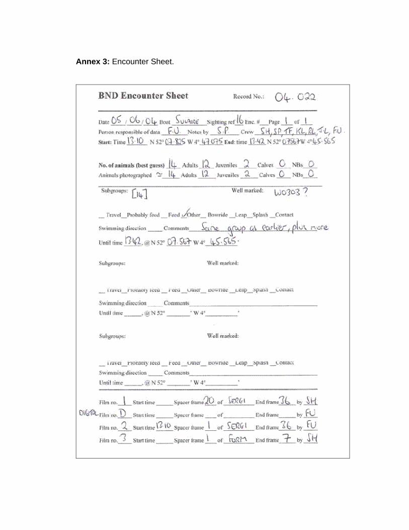
Annex 3: Encounter Sheet.

Annex 4: Film Sheet.

Annex 5: The results obtained from the (Mth) model for population sizes,
using CAPTURE run through MARK v4.1, for the years 2003, 2004 and 2005,
respectively.
2003 Input---title='2003 population'
Input---task read captures x matrix occasions=38 captures=38
Input---data='Group 1'
Input---format='(a6,38f1.0)'
Input---read input data
Summary of captures read
Number of trapping occasions 38
Number of animals captured 95
Maximum x grid coordinate 1.0
Maximum y grid coordinate 1.0
Input---task population estimate mth-chao
Population estimate under time variation and
individual heterogeneity in capture probabilies.
See model M(th) of Chao et al. (1992).
Group 1
Number of trapping occasions was 38
Number of animals captured, M(t+1), was 95
Total number of captures, n., was 435
Frequencies of capture, f(i)
i= 1 2 3 4 5 6 7 8 9 10 11 12 13 14 15 16 17 18 19 20 21 22
23 24 25 26 27 28 29 30 31 32 33 34 35 36 37 38
f(i)= 16 15 12 8 9 10 7 6 6 3 2 0 1 0 0 0 0 0 0 0 0 0
0 0 0 0 0 0 0 0 0 0 0 0 0 0 0 0
Estimator Gamma N-hat se(N-hat)
--------------------------------------------------

1 0.2830 103.33 4.22
2 0.2806 103.09 4.17
3 0.2807 103.10 4.17
p-hat(j) = 0.11 0.10 0.08 0.12 0.11 0.09 0.16 0.14 0.07 0.10 0.17 0.11 0.04 0.13 0.05 0.10
0.10
0.08 0.11 0.10 0.19 0.20 0.20 0.11 0.17 0.10 0.12 0.14 0.17 0.07 0.03 0.10 0.18 0.07 0.04
0.11 0.07 0.14
Bias-corrected population estimate is 103 with standard error 4.1719
Approximate 95 percent confidence interval 99 to 115
2004 Input---title='2004 population'
Input---task read captures x matrix occasions=32 captures=32
Input---data='Group 1'
Input---format='(a6,32f1.0)'
Input---read input data
Summary of captures read
Number of trapping occasions 32
Number of animals captured 82
Maximum x grid coordinate 1.0
Maximum y grid coordinate 1.0
Input---task population estimate mth-chao
Population estimate under time variation and
individual heterogeneity in capture probabilies.
See model M(th) of Chao et al. (1992).
Group 1
Number of trapping occasions was 32
Number of animals captured, M(t+1), was 82
Total number of captures, n., was 242
Frequencies of capture, f(i)
i= 1 2 3 4 5 6 7 8 9 10 11 12 13 14 15 16 17 18 19 20 21 22 23 24 25 26 27 28 29
30 31

32
f(i)= 22 26 13 6 4 6 1 0 2 0 1 0 1 0 0 0 0 0 0 0 0 0 0 0 0 0 0 0 0 0 0 0
Estimator Gamma N-hat se(N-hat)
--------------------------------------------------
1 0.4618 101.38 8.15
2 0.4507 100.34 7.96
3 0.4513 100.39 7.97
p-hat(j) = 0.10 0.14 0.14 0.09 0.06 0.12 0.08 0.02 0.04 0.06 0.07 0.07 0.04 0.10 0.04 0.10
0.11
0.07 0.02 0.07 0.07 0.03 0.10 0.09 0.07 0.09 0.11 0.10 0.08 0.06 0.07 0.01
Bias-corrected population estimate is 100 with standard error 7.9722
Approximate 95 percent confidence interval 91 to 123
2005 Input---title='2005 BND population size'
Input---task read captures x matrix occasions=15 captures=15
Input---data='Group 1'
Input---format='(a6,15f1.0)'
Input---read input data
Summary of captures read
Number of trapping occasions 15
Number of animals captured 68
Maximum x grid coordinate 1.0
Maximum y grid coordinate 1.0
Input---task population estimate mth-chao
Population estimate under time variation and
individual heterogeneity in capture probabilies.
See model M(th) of Chao et al. (1992).
Group 1

Number of trapping occasions was 15
Number of animals captured, M(t+1), was 68
Total number of captures, n., was 115
Frequencies of capture, f(i)
i= 1 2 3 4 5 6 7 8 9 10 11 12 13 14 15
f(i)= 40 13 12 2 1 0 0 0 0 0 0 0 0 0 0
Estimator Gamma N-hat se(N-hat)
--------------------------------------------------
1 0.2442 119.24 19.24
2 0.2141 114.56 18.28
3 0.2204 115.53 18.49
p-hat(j) = 0.16 0.02 0.13 0.04 0.15 0.06 0.05 0.10 0.06 0.05 0.02 0.03 0.08 0.02 0.03
Bias-corrected population estimate is 116 with standard error 18.4891
Approximate 95 percent confidence interval 91 to 167