POPULATION, INCOME AND FOREST GROWTH:

MANAGEMENT OF VILLAGE COMMON LAND IN INDIA*

.

Andrew D. Foster

Mark R. Rosenzweig

Jere R. Behrman

Abstract

A newly-assembled data set that combines national household survey data, census data and satellite

images of land use in rural India over a 29-year period is used to obtain estimates of economic growth

and population effects on forests, to identify the mechanisms by which these factors affect land use, and

to address whether forest areas are efficiently managed where community land management is present.

The evidence suggests that increases in the returns to alternative uses of land induced by agricultural

technical change and population growth, combined with the difficulty of monitoring forest-resource

extraction, are the major contributing factors to deforestation.

*The research reported in this paper was supported in part by grants NIH HD33563 and NIH HD30907.We are grateful to Nauman Ilias and Joost Delaat for able research assistance and to two anonymousreferees and Edward Glaeser for helpful comments.

1In India, for example, Bowonder [1982] reports that 96 percent of the total forest areas isowned by the government.

1

I. Introduction

The growing concern about the phenomena of global warming and declining bio diversity has led

to an increase in attention paid to the disappearance of the world’s forests, particularly in the developing

world. Forests cover about 40 percent of land in tropical nations, and deforestation has been

especially acute in Asia. Between 10 and 20 million hectares of tropical forest are cleared each year,

with annual rates of deforestation between 1980 and 1990 averaging 1.2 percent in Asia, compared

with 0.9 percent in the developing world (Ehui and Hertel [1989]; World Bank [1992b]). The Asian

Development Bank (ADB) claims that "there are four major environmental problems ... arising from

population pressures, lack of development, and the development process itself" and three of these

four problems in Asia - "land degradation and depletion of natural resources; ...pollution of soil,

water and air; and consequences of global warming due to excessive discharge of green house gases

to the atmosphere" - are intimately associated with deforestation [Jalal 1993, p. 2].

While a variety of global economic forces affect the trends in deforestation in developing

countries, recent research has emphasized the importance of local-level processes such as agricultural

encroachment and product extraction through firewood collection and animal grazing that are themselves

importantly influenced by the fact that forest resources in most developing countries are not privately

owned (e.g., DasGupta [1995], Loughran and Pritchett [1997], Filmer and Pritchett [1996], Agarwal and

Yadama [1997], Jodha [1985], Ligon and Narain [forthcoming], López [1997]).1 The nonprivate

ownership of forests lands, as well as of grazing and waste lands, has raised questions of whether there

historically has been and/or currently is a "tragedy of the commons" that characterizes forest operations.

Several researchers, most notably Jodha, have investigated whether, in the absence of regulatory

institutions, rapid population growth actually leads to degenerative patterns of use and the gradual

depletion of common property resources (CPRs) (Chopra and Gulati [1993]; Jodha [1985, 1990]; Runge

2Sedjo (1995) provides a useful discussion of the differing trajectories of forest cover indeveloped and developing countries. He notes, for example, that the state of New Hampshire experiencedan increase in forest cover from 50 to 86 percent of total land area in the period 1850-1990.

2

[1981]; Repetto and Homes [1984]; Wade [1988]; White and Runge [1994]). Although as popularly

conceived depletion of such resources is a straightforward consequence of rapid population growth, these

studies suggest that traditionally many CPRs have been well-managed by local institutions so that

historically the effects of rapid population growth have been, in Jodha's [1985, p. 247] words, "mediated

by institutional factors and often overshadowed by pressures arising from changing market conditions."

Considerably less attention has been given to the related question of how income growth in

general, and technical change in agriculture in particular, has impacted forest resources. While it is

widely recognized that improvements in agricultural productivity permit population growth without

adverse Malthusian income consequences, the effects on forest resources of both population growth and

agricultural technical change remain an open question. Moreover, in the substantial economic literature

concerned with the question of the efficiency with which common areas such as forest areas are managed

in developing countries, there is surprisingly little discussion of the process by which forest area is

chosen. The primary difficulty with this approach, with its emphasis on tree management, is that it

neglects factors determining the demand for forest products and does not allow for the possibility that

forest area will be importantly determined by the relative returns to forest and other uses of land. These

omissions would seem difficult to justify in terms of current patterns of forestation and deforestation in

both developed and developing countries. In particular, growth in forests in the developed world in recent

years can be attributed in part to investment decisions on the part of private owners in certain regions

(such as the Northwest US) and to decreases in the returns to agriculture in others (such as New England)

that reflect the changing costs of labor, an important input in forest extraction, and changes in the

demand for forest products.2 An investigation of the determinants of deforestation thus needs to pay

attention to the markets for land, labor and forest products as well as land management.

One important barrier to improved understanding of the technological, behavioral and

3In a recent article, however, Cropper and Griffiths [1994] have assembled a data base consistingof a time-series of non-OECD countries over the period 1961-91 that serves to describe associationsamong forest land, per-capita GDP, and population density within major continents of the world.

4Cropper and Griffiths (1994) were unable to estimate any significant relationships for Asia orSouth Asia using official government statistics on forests.

3

organizational forces affecting global deforestation has been the absence of adequate data. Many

empirical studies of land and forest use are based on case studies over short time periods that do not

permit identification of the longer-term consequences of population change or technical progress and

cannot easily be generalized.3 In this paper, we utilize a newly-assembled data set that combines at the

village level longitudinal household survey data, Census data and satellite images of land use that cover a

wide area of rural India over a 29-year period to address limitations to knowledge about how agricultural

technical change and population growth affect land management in general and the management of forest

exploitation in particular. A key feature of the data is that while in many villages all land is privately

owned, a substantial number of the villages have common lands governed by the local village council

(panchayat). We use the data to obtain estimates of rural economic growth and population effects on

deforestation, to identify the mechanisms by which these factors affect land use, and to address the

question of whether forest areas are efficiently managed in areas in which community management of

lands is present.

India is a particularly interesting and useful setting in which to study the management of forest

resources. Over 20 percent of all land in India is designated as forest land, 96 percent of which is

publicly managed common land. Moreover, India is a country that has experienced rapid population

growth and since the late 1960's has been a major beneficiary of the “green revolution,” which has

substantially augmented crop productivity growth. Large-scale studies of the effects of agricultural

productivity growth or population change on forests in India have been limited, however, by the fact that

governmental data sources provide information only on designated forest lands, including newly-

designated land for forests on which tree planting may have only been recently initiated rather than on

actual tree coverage or forest biomass.4 Information on actual land use, based on satellite images, is thus

5The information on land use prior to 1999 is from Anon 1997, pp.90-91 and from the Food andAgricultural Organization for 1999. The earliest satellite images are actually for 1972. The constructionof the measures of forest growth are discussed below.

4

necessary to evaluate the effects on actual forest biomass of population trends and the agricultural

productivity increases.

Another reason that India is an important area of study is that there have been substantial efforts

to reforest starting in the early 1950's by subsidizing the provision of seedlings to be allocated and

distributed by village governments. Indeed, the efforts to increase forest growth stemmed from the notion

that increasing population would increase the demand for forest products (FAO, 1999). Figure I plots the

(i) proportion of land in India designated by the government as forest land for each Census year from

1951 through 1991 and for 1999 and (ii) our satellite-based estimates of the proportion of land of land

with trees surrounding the sample villages in our nationally-representative survey data for the same years

starting in 1971 when satellite data first became available.5 Contrary to popular belief, the government

statistics indicate that the amount of land both estimated to be forested and set aside for forests has

increased in India since 1951, rising from 12.3% in 1951 to over 23% in the 1990's. Moreover, our data,

based on satellite imagery for our national sample of Indian villages, indicate that the increase in set-

asides for forest land has been accompanied, with a lag, by increases in actual forests. These estimates

indicate that the proportion of land covered by forests increased from just over 10% in 1971 to over 24%

in 1999.

During the same 29-year period that forests surrounding our sample villages have experienced

growth on average, the average population size of the villages almost doubled and yields of the hybrid-

seeds associated with the green revolution have almost tripled. Moreover, as documented below, over the

same period the villages have electrified, access roads have substantially improved and factories have

been set up in almost all villages. This does not necessarily imply that rural economic development and

population growth have not adversely affected forests. These aggregate trends mask important

differences in the experiences of Indian villages. For example, 41% of our sample villages experienced a

6 In addition, it has been argued that reforestation has altered the nature of forest ecosystems suchthat bio-diversity has been reduced. For example, some local government forest programs involve thedistribution of seeds for specific tree species, such as eucalyptus and populus (FAO, 1999).

5

decline in forests between 1971 and 1999.6 To identify the roles of population change and rural

development and to assess the efficiency of local land management thus requires the comparison of the

changes in forests across villages over time with their changes in population size, agricultural

productivity and rural infrastructure.

Section II of the paper briefly describes the theoretical framework that guides the empirical

analysis, highlighting the mechanisms by which technical change in agriculture, rural industrialization

and population growth affect forest area and the demand for forest products and contrasting perfect-

markets and unmonitorable labor regimes to consider the effects of forest-management institutions on

these relationships. Section III describes the data sources and the construction of the variables. Section

IV presents the reduced-form estimates and Section V the structural estimates that identify the

mechanisms by which economic growth and population change affect forests and the role of land

management. Our results indicate that the effect of income growth on forests is importantly conditioned

by the specific mechanisms causing incomes to increase. Our structural estimates indicate that the

principal mechanism through which both agricultural technical change and population growth cause

deforestation is through their effects on pushing up the value of land for growing crops. Rural

industrialization has had little impact on forest survival because industrialization did not appear to raise

land rents appreciably, in contrast to the effects of the improvements in agricultural productivity, and

because changes in income per se appear to have only weak direct effects on forest exploitation. These

results suggest that the “green” revolution in India, while forestalling the negative income consequences

of a Malthusian equilibrium, was less green than first thought. Our estimates also are also consistent with

the hypothesis that the difficulty of monitoring the extraction of forest is a contributing factor, along with

agricultural technical change, to inhibiting the growth of forests.

II. Empirical Framework

7Bowonder (1982) estimates that 90 percent of the wood extracted in India is used for fuel.

6

To highlight the roles of both the demand for forest products and the changing opportunity costs

of land and labor in determining forest resources that arise from agricultural technical progress, rural

industrialization and population growth and to evaluate the role of constraints on land management in

affecting these relationships, we need an empirical framework encompassing three sectors - agriculture,

forestry, and industry - with two factors of production - land and labor. We assume that rural India can be

characterized as an economy composed of sub-economies (villages) which are locally governed and

across which there is little labor mobility. However, manufactured goods and agricultural products are

traded across villages and labor is freely mobile across sectors within villages. To capture the effects of

local demand for forest products we also allow for constraints on trading such products (firewood) across

villages, consistent with the observation that goods such as firewood or the forage consumed by livestock

in the forest, the principal uses of forest products in the Indian context that we study, are bulky and thus

are not easily transported.7 Thus, given that land is also immobile, wage rates, land prices and forest-

good prices are locally determined.

We consider three sources of economic growth and productivity variation in the three sectors that

affect the supply and demand for resources in each village: changes in technology in the agricultural

sector that vary across areas due to differentials in the suitability of and constraints on the adoption of

high-yielding variety crops, naturally varying local environment variables (rainfall, temperature, soil

quality, etc.), and variation in variables affecting labor productivity in the manufacturing sector (the

availability of infrastructure, capital, and knowledge relevant to the generation of non-agricultural non-

forest employment). How these exogenous factors and population growth affect the land allocated to

forests will depend importantly not only on the technology of production and the preferences of

households but on the institutional structure governing resource allocation. We contrast two cases that

incorporate different constraints on forest management and discuss how these cases may be distinguished

empirically.

8We are assuming for simplicity that households are identical and that time periods are ofsufficient length such that the extraction of forest resources in one period does not influence the output offorest products in subsequent periods,

7

A. Input and Output Markets and the Efficient Allocation of Land

We consider first a benchmark case of complete and perfect input and output markets to examine

how shifts in population size and technical change influence forest use when inputs are allocated

efficiently. This “complete-markets” framework thus corresponds to a setting in which all labor can be

monitored and either all land, inclusive of forests, is privately held by each household or, equivalently,

any forest-land commons are first-best efficiently chosen and managed by a village council or other

institution. We assume that households maximize utility and in each period choose allocations of land to

forest and agricultural production, allocations of labor to forest-product extraction, agriculture,

manufacturing, and the labor market, and the consumption of forest and non-forest goods.

Solving the first-order conditions determining the allocation of labor and land along with the

equilibrium conditions for labor markets and forest products yields reduced-form expressions for how

forest area as well as the opportunity costs of forest-product inputs - wages and land rent - are influenced

by agricultural technology improvements, changes in infrastructure, endowment income, and population

density, as determined by variation in the number and size of households. In this simple framework8

agricultural technical change, population growth and rural industrialization have quantitatively and

perhaps qualitatively different effects on forest survival, even if they have similar effects on the demand

for forest products, because they differentially affect the opportunity costs of the two main forest inputs,

land and labor.

The effects of improvements in (factor-neutral) agricultural technology on land rents and wages

in this framework is straightforward - both increase as agricultural productivity rises. The effects of

population growth are more complex. Because the household is the decision-making unit, the effects of

increases in household size and density (the number of households per unit area) on land rents and wages

may differ depending on the existence of scale economies in consumption and production. For given land

8

area per household (total number of households), the framework predicts that increases in the size of

households and thus the total population will increase land rents and lower wages. Controlling for total

population, however, increases in the total number of households population will lower (raise) land

prices if there are production scale economies (dis-economies). In the case of the determination of

household income, different effects of household size and density are especially likely to be observed

because increases in household size directly increase household income, although less than

proportionally, by augmenting household labor supply. Finally, manufacturing productivity raises wages

and may raise or lower land rents depending on how such change affects the demand for forest products.

Despite the fact that the effects of agricultural technical change and population growth have

predictable effects on the two components of the opportunity costs of forest land use it is not possible

even in this simple framework to derive a prediction as to how in the reduced-form changes in

agricultural technology, population growth or changes in conditions that promote the expansion of the

manufacturing sector affect the forest allocation. It is thus an empirical question as to whether and how

agricultural technical change and population growth contribute to deforestation.

The principal reason for the ambiguity with respect to even the consequences for the land

allocated to forests of advances in farm technology is that the effects of changes in the opportunity cost

of labor used to extract forest products and of changes in income that affect the demand for forest on the

forest allocation cannot be predicted. This framework can be used to derive equilibrium conditions that

relate the two endogenously-determined cost variables - wages and land rents - and endogenously-

determined incomes along with the population variables to the optimal forest allocation. These indicate

that while increases in the opportunity cost of land, induced by both technical progress in agriculture and

by population growth, unambiguously reduce the amount of land allocated to forests, the sign of the wage

rate effect on forest area is ambiguous, depending on the price elasticity of demand for forest products

and properties of the production technology. And, of course, the sign and magnitude of income effects

induced by technical change and population growth depend on the exact nature of household preferences

9This results depends importantly on the absence of dynamic effects of current forest use onfuture output over a long time period. The test can be generalized, however, to take into account differentassumptions about saving and/or borrowing opportunities by replacing income with householdexpenditures as long as any uncertainty is resolved prior to the making of decisions.

10Note that the signs of the income and family size effects on the demand for forest products arenot known a priori, and must be estimated. Because firewood, for example, may be considered an inferiorfuel, increases in income may result in lower demand for firewood. Similarly, increases in household sizemay increase or decrease demand depending on the extent to which firewood serves as a public good forhousehold members as well as the price elasticity of demand for that commodity.

9

for forest products.

B. Common-Land Management and Unmonitorable Labor

The benchmark model sketched above in which forest products are treated like a conventional

crop provides a sensible way of capturing the idea that forest area will be importantly determined by the

returns to alternative uses of land and by pressures on wage rates. While this approach does not provide

an explanation for key institutional features of forests such as that they are frequently held in common

land, it should be emphasized that the approach does not necessarily assume that forest land is privately

held. The market solution could emerge if forests were commonly owned as long as both the area and

usage of these forests were first-best efficiently chosen and managed.

There is an important restriction that arises from the complete-markets framework, however. In

particular, in the aggregate the signs of the partial effects of income and household size on forest area,

conditional on the market wage rate and land price, are the same as those that would be observed in

household forest product demand equations.9 This strong prediction implies that estimation of the effects

of household size and income from the market equilibrium equations that condition on wage rates and

land prices, given information on the effects of household size and income on household forest-product

demand, can provide a test for (local) market completeness, inclusive of the efficient management of

forest resources.10

In order to assess whether the restrictions from the first-best allocation model concerning the

effects of the income and family size variables on forest area net of wage rates and land prices in

equilibrium provide a test of first-best allocations requires an alternative model. A reasonable candidate

11Filmer and Pritchett, for example, report that 34 per cent of firewood in rural Pakistan iscollected from land held privately by other households without compensation.

12It can be shown that at the social-planner's optimal allocation of forest land, the marginalrevenue product of forest land exceeds the marginal revenue product of agricultural land so that, giventhe prevailing wage and land rental rate and the marginal products of land and labor in forests, there istoo little forest land and too much extraction of forest resources per unit land compared to thecompetitive case.

10

is a model in which forest area is selected to maximize some welfare criterion subject to constraints that

preclude the implementation of first-best outcomes. One constraint that is highlighted in the literature,

given the apparent important of common-management of forest resources, is the high cost of monitoring

the extraction of forest resources. The idea is that given the land intensity of forest goods production and

the fact that visibility may be obscured in forested areas, even privately owned forest resources would be

subject to a “commons tragedy.”11 An obvious but significant implication of the assumption that forest

extraction cannot be directly monitored is that households would not wish to hold any land in forests as

they would be unable to extract rents from such property. Given the high costs of transporting forest

resources it is thus in the interest of the village as a whole to set aside some amount of land as

commonly-held forests. Although the amount of land that is thus held, to the extent that it is chosen

optimally, will be importantly influenced by the marginal productivity of land, it will not, in general, be

chosen as in the benchmark case so that the marginal revenue product of forest land is equal to the

equilibrium price of land as determined in the agricultural sector given forest labor.12

In the framework in which labor is unmonitorable but all inputs are optimally allocated subject to

the monitorability constraint, in contrast to the complete markets regime, the system of equations

determining equilibrium in the forest-products sector cannot be decentralized, so that forest area cannot

be solved as part of a three-equation system conditional on wages, rentals, and household income. This

implies that the restrictions on the forest-area equilibrium conditions are unlikely to hold in this

alternative regime. However, the analytic derivation of comparative static results is also prohibitively

complex. In Foster, Rosenzweig, and Behrman (1998) we show that for at least one parametric

specification of this alternative model, the test of the restrictions associated with the complete-markets

13For example, using village-level samples from specific sub-regions of India both Jodha (1985)(Western Rajasthan) and Agarwal and Yadama (1997) (Kumaon Himalaya), find evidence of arelationship between forest conditions and village-level resources and institutions.

11

regime have power against the alternative of unmonitorable forest labor. Moreover, this model indicates

that under conditions in which the demand for forest products, conditional on the forest-good price, is

increasing in household income and not affected by household size, increases in both household size and

household income can have a negative effect on aggregate forest area net of wages and land prices. Thus,

in this particular parametric specification, the consequences of increases in both household size and

household income for deforestation, net of wages and land prices, are more adverse when forest area is

second-best efficiently managed than in the case in which land is efficiently managed.

III. The Village Panel Data Set

As noted, India represents an interesting and potentially useful setting in which to examine the

determinants of forest growth and the role of market failures in determining the management of forest

resources. The spatially-differentiated growth in agricultural productivity resulting from the exogenous

importation of new seed technologies applied to differentially-suitable agroclimates combined with the

relatively high rates of population growth experienced by India in the over the past 30-40 years would

appear to have the potential to provide insights into the roles of agricultural technical change and

population growth in affecting the levels of and changes in forest area.

Given the existing evidence that villages in India play a prominent role in the management of

forest resources,13 we have constructed a panel data set at the village level for approximately 250 villages

covering the period 1971-1999 that combines multiple sources of data, that conforms to our multi-

sectoral framework and that incorporates heterogeneity in the organization of land management. In

particular, we have merged survey-based information on crop productivity, household incomes,

household consumption, household size, numbers of households, land prices, wage rates, rural

electrification, roads, and industry presence with governmental statistics on weather and satellite-based

information on locale-specific changes in the density of forests. The constructed data set comes from six

14Roughly speaking, the high infra-red reflectance accounts for the relative coolness of vegetationand the low red reflectance accounts for the green color.

15Although the NDVI is thought to be a good measure of photosynthetic activity, the relationshipbetween this measure and characteristics of forest cover such as biomass, carbon content, or leaf area isnot completely straightforward (Wulder [1998]). It has been established, for example, that the top layerof leaves effectively mask the presence of leaves at lower levels thus yielding a non-linear relationshipbetween the NDVI and leaf area. Moreover it is sometimes difficult to distinguish forest area fromagricultural crops. We address that issue through our selection of the timing of images, as discussedbelow. It is, however, not clear that any single measure clearly dominates the NDVI in terms of being

12

sources: (i) the 1970-71 National Council of Applied Economic Research (NCAER) Additional Rural

Incomes Survey (ARIS), (ii) the 1981-82 NCAER Rural Economic Development Survey (REDS), (iii)

the 1991 Indian Census, (iv) the 1999 NCAER Village REDS, (v) the National Climate Data Center

monthly global Surface data, and (vi) satellite spectral images for India from 1972-1980, 1992 and 1999.

A. Measuring Forests

As noted, official Indian data sources for the period spanning the three NCAER surveys provide

information on land officially classified as forest. This includes land newly set aside for growing trees

but which may not yet exhibit any vegetative growth as well as designated forest areas that have been

encroached upon by local growers. The absence of ground-level censuses of trees for the relevant period

covered by the survey means that in order to obtain a measure of the changes in actual forest or tree cover

for the specific “micro” regions surrounding each of the survey villages it is necessary to employ satellite

images. Satellite images based on specific light-frequencies enable the construction of indices that

measure reasonably accurately area vegetation for relatively small geographic areas. The index we use is

the normalized differentiated vegetation index (NDVI) (Rouse et al [1974]), which is the ratio of the

difference in reflectance in the near infra-red and red bands in the light spectrum to the sum of these

reflectances. This index correlates well with the presence of plant matter because vegetation tends to

reflect infra-red light and absorb red light.14 It is among the most commonly used measures of vegetative

cover because it is simple to compute and filters out topographic effects, variations in the illumination

angle of the sun, and other atmospheric elements such as haze. The NDVI is bounded between -1 and 1,

with vegetation associated with trees achieving values of .2 or greater.15

able to provide a robust measure of forest area across a wide variety of areas and climatic conditionsgiven the nature of available remote sensing data from the period in question. Moreover, errorsassociated with the use of NDVI to measure forest cover that are fixed over time in particular areas willnot importantly influence our results when we examine differential changes in the NDVI across regions.

13

To match the satellite and survey data we first geo-coded the survey data. To do this we obtained

geographic position codes for the ARIS survey villages based on maps from the district-level volumes of

the 1971 and 1981 Indian censuses. To ensure that survey village names corresponded to those in the

census, we used the survey information on village, tehsil, and district names. Seven villages had to be

dropped from the original 250 because a village of the name specified in the ARIS sample was not found

(4 of 7) or because more than one village of the same name was found in the corresponding tehsil and

district (3 of 7). The tehsil maps, which plot the locations of each village, were then geo-registered using

the district-level maps, which contain latitude and longitude information.

Measurement of forest cover for each of the sample villages that could be linked to the

corresponding time periods involved accessing three distinct sources as discussed in detail below:

Multispectral Scanner (MSS) images from Landsats I-III for the period 1971-1982; Advanced Very High

Resolution Radiometer (AVHRR) NDVI data from 1992 compiled by the USGS; and Extended Thematic

Mapper Plus (ETM+) images from Landsat VII for 1999. The two primary summary measures used for

the distributions of NDVI within a 10km radius of each sampled village were the proportion of pixels

with an NDVI>0.2 (NDP) and the mean NDVI of those areas with an NDVI exceeding 0.2. The product

of these two measures was also constructed as a measure of overall biomass attributable to forests

(NDT).

The MSS images have a spatial resolution of approximately 80 meters in four bands of the

spectrum. Each “path” and “row” pair uniquely determine a geographical area of approximately 185 kms

square for the MSS images. A number of criteria were used to select specific scenes. First, it was

desirable to have scenes for each location that corresponded as closely as possible to the crop-years

covered by the ARIS (1970-71) and REDS (1981-1982) surveys. The most important constraints in

matching by crop-year are that the first Landsat satellite, Landsat 1, was not launched until late in 1972

14

and the availability of the relevant scenes for India is limited after 1980. Second, in order to control for

seasonal variation in vegetative cover, scenes were selected for a given area that were at similar points

within the crop-cycle and corresponded to periods within the year during which there is minimal

presence of standing crops, which can be difficult to distinguish from forest area using satellite imagery.

Preliminary analysis suggested that the months of January and February were best. Third, because areas

covered by clouds cannot be used to assess vegetative cover, images were selected with little or no cloud

cover. The choice of the winter months was also useful in this regard because the cloud-laden monsoon

period was excluded.

We were reasonably successful in meeting all of these criteria. Ninety-six percent of the scenes

corresponding to the ARIS survey came from late 1972 and early 1973, with the scenes corresponding to

the REDS survey distributed between years 1977 and 1980. The average number of years between these

scenes across path-row combinations is 5.1, with 75 percent of the observations spanning the interval

between 4 and 7 years. In addition, 81 percent of the selected scenes came from January and February,

with all scenes coming from the November-April period. Finally, the level of cloud cover for the selected

scenes never exceeds 2 on a 0-7 scale, with 0 denoting complete absence of clouds and 7 complete cloud

cover.

For each of the selected 146 scenes corresponding to a specific path-row-day combination we

obtained positive transparency images for both the near infra-red and red bands of the spectra. These

images were then scanned at a resolution of 300 pixels per inch. Images were then registered to latitude

and longitude using data on the locations of the four corners of each image. The intensity of the images

was then adjusted using the grey-scale bands printed on the side of each image. Scans of these two

images were combined to construct a measure of NDVI for each of 6.5 x 106 pixels in each scene. Based

on these, we obtained a distribution of the values of the NDVI pixels within a 10km radius of each

village for each of the surveys. On average there were 53,904 pixels within the desired radius for each

village.

16This arises from the non-linearity of the forest-cover measure. Consider, for example, a 10kmradius image consisting of 50,000 pixels, 40 percent of which have an NDVI of .3 and 60 percent ofwhich have an NDVI of .4. At this resolution our measured forest cover (NDVI>.2) is 40 percent. Nowsuppose the image is degraded by a factor of 100 so that the village now contains 500 pixels. In theextreme case that the forest and non-forest pixels are independently distributed across the village then,using the same .2 cutoff one would obtain a forest cover measure of only 3.6 percent.

15

Selection and analysis of the Landsat VII images from early 1999 followed a roughly similar

procedure, with the exception that images were available digitally making it unnecessary to manually

geo-register and intensity-correct the images. Coverage of the relevant villages required 85 distinct path-

row combinations for this satellite. Images were selected to have low cloud cover and correspond to the

time-period of the year for the early images. The images are at a resolution of 30 meters but were

resampled to a resolution comparable to that of the 1971-1982 images before the NDVI measures were

calculated. The selected Landsat VII images were collected between November 1998 and April 1999 and

had cloud cover of less than 20 percent.

Due to the limited availability and high cost of Landsat images for the South Asian region during

the 1980s and early 1990s, an alternative source was used to construct NDVI measures to correspond to

the 1991 Indian census. In particular, we obtained NDVI images compiled by the USGS based on data

collected from the AVHRR satellite in 1992. Because these images have a lower resolution (1.1

kilometer) than the Landsat images and because measures of vegetative cover may be importantly

affected by the resolution used16 we resampled these images to a higher resolution based on the content

of the 1999 images. In particular, selected 1999 images were first sampled to a resolution of 80m and

then averaged to a resolution of 1km. We then constructed a linear regression equation relating NDVI in

the 80m images to that in the 1km images for 1999 and determined the variance of the resulting residual.

This regression equation combined with random draws from the corresponding error distribution were

used to construct NDVI images with a nominal resolution of 80m based on the original 1km AVHRR

images.

B. Village-level Economic and Demographic Variables

The national NCAER surveys and the 1991 Indian Census village-level data provide information

16

on variables describing the economic environment of the villages matched to the satellite data on forests

over the 1971-99 period. The 1970-71 round of the ARIS data provides information on household

structure (age-sex composition); income by source, agricultural inputs, outputs and costs, by item, and

wage rates and labor supply for 4,659 households in 259 villages that were selected based on a stratified

random survey design. The data set contains sample weights reflecting the stratified sample design so

that population statistics, necessary for aggregation and merging, can be obtained from the survey data.

Also provided is information on village population size, village-level land prices, for irrigated and

unirrigated land, and on village infrastructure, including whether the village was electrified and the

presence of rural industry and whether or not the village was located in a district participating in the

Intensive Agricultural District Program (IADP), a national program instituted in the late 1960's that

provided agricultural resources and subsidies of agricultural input (seeds, fertilizer)in areas believed to

be those that would be subject to the most significant productivity improvements as a consequence of the

green revolution..

The 1982 REDS data provide similar information for the 1981-82 crop year on a subset of the

original 1970-71 households as well as data on a new, random sample of households based on the same

survey design as in the ARIS and on a complete census of households in the original 259 ARIS villages.

However, because of political constraints, all households in the state of Assam were dropped from the

sampling frame. The panel and the new households together number 4,947 and, based on the sample

weights, are representative of the entire national rural Indian population (except for Assam) in 1981-82.

The REDS data also provide sampling weights for all households, as described in more detail in

Vashishtha [1989], thus permitting construction of a representative data set at the village level for 1981-

82 that can be matched with that from 1970-71. In 1999, NCAER under our direction carried out a survey

of the same villages as in the 1970-71 ARIS, excepting those in Jammu and Kashmir states, collecting

information consistent with that collected at the village-level in 1982.

To construct a measure of agricultural technology, information from the three surveys on crop

17The sources for village population sizes for the ARIS and the 1981-82 REDS surveys were the1971 and 1981 Censuses of India. Surprisingly, a non-trivial number of the villages in the Census data donot report population or household size. The fraction of non-reporting villages for the years 1971, 82, 91are .055, .279, and .051, respectively. Population estimates for the 1999 village survey are missing for13.1% of the villages. Similarly, 12.4% of the villages in 1991 and 15.7% in 1999 had no information onnumber of households so that it was not possible to compute average household size. In the econometricanalyses reported below, we include observations with missing values for population and household sizeby setting the missing values to zero and adding to the specification dummy variables indicating thatthese variables were not available.

17

outputs and acreage planted by crop, type of land and seed variety (high-yielding (HYV) or not) was used

to construct a Laspeyres index of HYV crop yields on irrigated lands combining four HYV crops (corn,

rice, sorghum and wheat) using constant 1971 prices for each of the villages for the three survey years.

The 1970-71 ARIS and the 1981-1982 and 1999 REDS data sets thus provide a consistent set of rural

agricultural wage rates, land prices, HYV crop productivity, and rural industry measures and information

on the size and numbers of households for up to 253 villages spread all over India for the years 1971,

1982 and 1999. We also obtained information from the 1991Indian Census on a subset of the 1999

survey villages. The Indian Census provides data for every village in India on population size, number of

households and road types for 1991.Using as matching information village, tehsil and block names we

were able to match 234 of the 253 villages in the 1999 survey.17 The 1999 REDS provides histories of the

electrification of villages, which were used to determine which of the villages were electrified in 1991.

Based on the village geo-codes, we also matched information on annual rainfall to each of the villages in

each of the four relevant years using information on the nearest weather station from the set of 30

weather stations reporting data to the National Climate Data Center over the 29-year period. Figure 2

maps the location of the survey villages as well as the weather stations.

Table 1 provides the means and standard deviations for all variables for each of the four years,

along with the data source for the variables, and the number of villages in each round for which there is

survey or Census data. As can be seen, the data indicate that India experienced economic development

over the 29-year period spanned by the data: HYV crop productivity more than tripled, real agricultural

wages grew by 150%, the proportion of villages that were electrified rose from less than a third in 1971

18Bardhan [1993] discusses the notion that incentives to undertake group management ofcommon resources may be importantly related to local ecological conditions. Narain [1999] presentsevidence that the costs of monitoring forest resources is closely related to the degree of forestdegradation and considers the implications of this relationship for group management of resources.

18

to almost 93% in 1999, and the proportion of villages with a factory increased from 14% to 95%. At the

same time the average population of the villages increased by almost 91.7% and the proportion of land

with forest more than doubled.

An important feature of the 1999 survey data is the identification of those villages with common

or local-authority (panchayat) governed lands. Approximately 56% percent of the villages had village

commons, so that it is possible to examine the relationship between forest growth and property rights

and, in particular, carry out the tests, described above, of efficiency in the management of forest

resources. In particular, we can assess whether the estimates of the equilibrium equations more closely

conform to the restrictions of the first-best model in villages in which there is no common land compared

with villages with joint management of forest resources, presumably established as a response to the high

cost of labor monitoring.18

Table II provides information on forest area and density, population, crop productivity, wage

rates and prices from 1971 through 1999 for the sample villages stratified by whether or not they had

locally-managed common lands. The figures indicate that the proportion of land area devoted to forests in

the initial period was 39% higher in common-land villages compared with those villages without

government-controlled land. Villages with common lands also had agricultural land that was almost 8%

more productive than villages without common lands. The fact that common-land villages in 1971 had

both a greater proportion of land under forest and greater crop productivity than villages without

common lands might suggest that common-land governance succeeds in protecting forests despite high

returns to alternative land use. However, it is also possible that conditions favoring crop productivity also

favor tree growth, or that forest land is of lower quality than crop land such that where more land is

devoted proportionally to agriculture, average crop productivity is lower. Given land and climate

heterogeneity, it is not possible to distinguish between these hypotheses from cross-sectional

19

associations.

Table II also indicates that forest cover increased slightly more in the common-land villages over

the last 29 years - the proportion of land covered by forest grew by 135% in common-land villages and

by 114% in the other villages. However, crop productivity growth in the villages with common land was

41.9 percentage points slower than that in the common-land villages. This suggests, in contrast to the

cross-sectional relationships in 1971, that the inability to monitor and enforce forest exploitation in the

face of rural economic growth may have attenuated forest growth. However, common-land villages

experienced faster population growth compared with the other villages over the same period. A more

systematic examination of the roles of population and economic growth in affecting the change in forests

is thus needed that takes into account land and climate heterogeneity and the interrelationships among

population, technical change, and the demand for forest products in assessing the efficiency of common-

land forest management and identifying the consequences for forests that emanate from improvements in

agricultural productivity.

IV. Estimates of the Effects of Productivity Growth by Sector and Population Growth

on Factor Prices, Income and Forests

We first estimate log-linear approximations to reduced-form equations relating the variation in

agricultural productivity, population size (number of households and household size) and rural

infrastructure (electricity availability and access road quality) to the equilibrium values of the village

wage, agricultural land price, average household income, factory presence and the measures of forest

coverage. The reduced-form estimating equations are given by

(1)

where z = r, the log of the average price of land in the village; w, the log of the village male agricultural

wage rate; y, average log of household income in the village; presence of a factory, and Af, the share of

village land area under forest and forest density, measured both by NDP and NDT, respectively. 2 t is an

index of agricultural productivity, measured by the four-crop productivity index; 0, represents industrial

19The relevant years for the reduced-form wage and land price equations are the NCAER ARISand the two REDS survey years (1971, 1982 and 1999). The income equations are estimated using datafrom 1971 and 1982, because the 1999 village survey does not provide household income measures. Forthe forest area equations, the relevant years are those for which we constructed the satellite-based forestmeasures. As noted, these do not exactly correspond to the first two survey years, 1971 and 1982. Tocontrol for the variation in the time-span between the satellite observations across villages, a variable wasincluded in the forest equations that measured the difference in years between the years of the survey andthe year of the forest observation.

20Note that prices of traded (across villages) inputs and outputs are impounded in the constantterm bzt and the year effects bzt. Differential changes across villages in prices due to changes intransportation technology, for example, might induce bias due to the omission of such prices, but only tothe extent that they are correlated with other included variables.

20

infrastructure and is measured by dummy variables indicating whether the village was electrified and had

a paved access road; et represents actual weather conditions at time t and is measured by the annual

amount of rainfall in the nearest weather station;19 lt is the average log of household size in the village,

and Nt is the log of the population in the village, tt is a set of dummy variables capturing year effects.20

Finally, < captures village-specific attributes of weather and soil as well as proximity to urban areas and

markets, and ,zt is a time-varying, village-specific shock.

As the relationships in Table II suggest, estimation of (1) by ordinary least squares (OLS) using

variation across villages at one point in time may be misleading because the unmeasured environmental

variable <, capturing time-invariant agroclimatic conditions and proximity to urban areas, influences

prices and incomes, and is likely to be correlated with agricultural productivity, the presence of industry

and the density and size of forests, including errors in the NDVI-based measures of forests. We exploit

the fact that we have data from multiple time periods to eliminate all such fixed effects by adding to (1)

village dummy variables. We also include dummy variables for the survey/census years to capture

aggregate trends in the variables.

Net of village and year fixed-effects the time-varying errors ,it in (1) representing, for example,

period- and village-specific productivity shocks other than rainfall in the two time periods may jointly

affect forest biomass, wages and incomes as well as crop productivity (e.g., forest fires that naturally

decrease forest area, increase the supply, and thus lower the price of arable land and average crop

21

productivity if the new land is less productive). In addition, our estimate of village crop productivity

likely measures with considerable error true agricultural productivity. We thus use instruments to predict

the village-specific changes in crop productivity. We exploit three characteristics of the green revolution

in India to assemble our instrument set. First, climate conditions across India make some areas of India

substantially more suitable for growing rice, while other areas are suitable for growing wheat but not rice

(ICAR, 1978; ICAR 1985). In 1971, 46% of the sample villages did not grow wheat and 32% did not

grow any rice. In those areas not growing wheat, over 45% of land was devoted to growing rice while in

the villages not growing rice, on average 18% of crop land was planted with wheat.

A second characteristic of the green revolution is that advances in productivity varied by crop. In

particular, technological advances in yields for wheat preceded those for rice but slowed more than did

those for rice in the later period, so that the areas differing by crop suitability experienced differential

advances in crop productivity (Evenson and David, 1993). To capture these crop-specific yield growth

differentials we used as instrumental variables predicting the growth in the HYV-crop index over the

1971-99 period the proportion of land in the village devoted to rice and wheat in 1971, respectively,

multiplied by year dummies. Finally, we used a variable representing whether or not the village was

located in an Intensive Agricultural District Program (IADP) district. The IADP was initiated in the late

1960's in one district in each Indian state to promote the adoption of the new seed varieties of the green

revolution through information dissemination and credit subsidy. This variable is thus unlikely to be

correlated with the initial crop productivity shock in 1971 but should be a good predictor of agricultural

productivity growth at least in the first decade of the sample.

Table III reports OLS and village fixed-effects (FE) estimates of the predicting equation for the

log of the crop productivity index. F-statistics indicate that the complete set of variables and the set of

instruments explain a statistically significant proportion of the variability in HYV yields across the

villages over the three sample periods. The estimates appear to capture the main attributes of the green

revolution, mainly the early productivity growth for wheat yields and the more rapid advancement for

22

rice yields later in the period. The OLS estimates indicate that in 1971 wheat yields were almost 50%

higher than rice yields but according to the FE estimates, which eliminate the influences of permanent

differences in soil and climate conditions across villages, both rice and wheat yields did not advance as

strongly over the 1971-82 period compared with the other two crops in the HYV yield index corn and

sorghum, with wheat yields evidently not advancing at all over that period. In the 1982-99 period, wheat

yield growth though positive was less than half that of corn and sorghum, while rice yields increased

substantially more than the other three HYV crops composing the yield index. The FE point estimates

suggest that rice yields in 1999 were four times those in 1971 while wheat yields were less than double

what they were at the beginning of the sample period. The FE estimates also indicate that village

electrification on average raised yields (on irrigated lands) by 24%.

The cross-sectional (OLS), fixed effects (FE) and instrumental-variables fixed-effects (FE-IV)

estimates of the reduced-form land price, wage and income equations (1) are provided in Table IV. The

estimated effects of increases in crop productivity on the prices of the two forest inputs, land prices and

wages in Table IV, whether estimated using the cross-sectional data only and with or without

instruments, conform to the relationships that are derived from the standard complete-markets framework

- increases in crop productivity increase both the price of land and the price of labor, and also increase

average incomes. The two estimates of agricultural productivity effects on the land price and wage based

on the specification including village fixed-effects are substantially smaller than those estimated based

on the cross-section, consistent with the existence of unmeasured land productivity factors that persist

over time. Of the two FE estimates of agricultural productivity on the two input prices and on incomes,

those obtained using the instruments are larger in magnitude, consistent with the existence of

measurement error, and are estimated with precision except for the productivity effect on agricultural

wages.

The FE-IV point estimates of agricultural productivity effects suggest that exogenously

increasing crop yields by 75%, roughly the increase in the first decade of the green revolution in India for

21Our reduced-form estimates of agricultural technology effects on wages are comparable tothose obtained by Evenson (1993) for North India based on district-level data over a comparable period -his results indicate that an increase in productivity raises wages by 19 percent. Evenson’s North Indianelasticity estimates also indicate, however, that agricultural productivity growth lowers land rents.

23

the four HYV crops, doubles land prices, increases rural agricultural wage rates by 4 percent and raises

agricultural incomes by 26%.21 The relatively small estimated effect of yield growth on wages may

reflect the fact that labor is mobile, so that local changes in crop productivity on wages may understate

the national effect. That labor mobility may be a factor affecting wages is suggested by the finding that

increasing the quality of the village’s access road increases the average wage in the village - agricultural

wages are almost 12% higher in villages with a pucca road. However, improvements in village

accessability also increase the probability that a factory is built in the village, which presumably

increases the local demand for labor. The estimates in the last column suggest that villages with paved

access roads are 15% more likely to have a factory. Improved village access also evidently increases the

local price of land - land prices are over 22% higher in villages with pucca access roads.

The reduced-form estimates of the effects of population growth, for given household density, are

also in conformity to the market framework when the fixed attributes of villages are taken into account.

The effect of changing population size, given area per household, is the sum of the log household and log

population coefficients. This sum is positive for the land price and negative for wages, as expected, when

fixed effects are included in the specification. The FE-IV point estimates suggest that a doubling of the

population would, in the absence of production scale economies, push up land prices by 48% (.764-.283)

and depresses wages by 21% (-.118-.0898). Increases in the number of households (increasing total

population for given household size), however, decrease land prices (and wages), suggesting that there

are scale economies in production. The FE-IV estimate in the household income equation suggests that a

doubling in household size, for a given number of households, increases household income by 80

percent. The estimate thus implies that doubling household size, for given agricultural technological

progress, reduces per-capita incomes by 20 percent.

The different qualitative and quantitative estimated effects of agricultural productivity increases,

22The negative FE and FE-IV estimates of the relationship between crop productivity and ourmeasures of forest density suggest that the growth in the values of these measures over time do notsimply reflect the fact that we have not been successful in distinguishing tree foliage growth from cropgrowth.

24

rural infrastructure and population growth on input prices and income indicated in Table IV, in general

conformity to the market framework, suggest that these growth factors will have different effects on

forests, to the extent that opportunity costs of land and labor use and incomes affect land allocations.

Table V reports the reduced-form OLS, FE and FE-IV estimates for the two forest-area measures. The

differences among the OLS, FE and FE-IV estimates of crop productivity effects are again consistent

with the presence of heterogeneity in soil productivity and measurement error in our productivity

measure. The cross-sectional OLS estimates suggest that areas with high crop productivity also tend to

have more area devoted to forest and more forest biomass. In contrast, the two sets of FE estimates,

which control for soil productivity and other fixed factors of the villages, indicate that increases in

agricultural productivity growth have negative effects on forest change, with the FE-IV productivity

estimates larger in absolute value than the two corresponding FE estimates.22 Indeed, the FE-IV point

estimates suggest that a 50% increase in crop productivity, for given number and size of households,

would reduce the proportion of forested area (NDP) by about 64 percent and forest density by about 76

percent. Thus while technological change in agriculture evidently forestalls the Malthusian income trap

by increasing wages and income (Table IV), it reinforces any destructive effects of population growth on

forests.

The population and household size effects on forests, like the estimates for crop productivity,

suggest the importance of the opportunity costs of land for forest growth. While the OLS estimates

indicate that population size and forest density are positively correlated, the FE-IV estimates, which take

into account measurement errors in crop productivity and differences across areas in inherent land

productivity that may attract population and facilitate vegetation, suggest that like crop productivity

improvements increases in the size of the population lead to deforestation. The point estimates indicate

that a doubling in population, leaving land parcels at the same size, would decrease the proportion of land

23In villages that were electrified in 1999, only 46.6% of the households used electricity.

25

forested by 14% ((-.122+.088)/.239) and forest biomass by 28% ((-.0419+.0187)/.0842).The estimates

also suggest, however, that increases in household density for given household size, which evidently

lower the average value of crop land (Table IV) and may also increase the demand for forest products,

leads to forest growth. The point estimates indicate that increasing the number of households by 50%,

while leaving household size constant, for example, would increase the proportion of land forested by

18% and increase forest biomass by 11%.

Finally, the FE-IV estimates provide a mixed picture for the effects of rural infrastructure

development and industrialization on forests. The Table IV estimates indicate that both electrification

and road improvement accelerate rural industrialization, but in Table V, although electrification appears

to augment forest growth, road improvement appears to accelerate deforestation. The difference may

suggest that villagers directly substitute electricity for fuelwood.23

V. Estimates of the Equilibrium Equations: Opportunity Costs

and The Efficiency of Common Land Management

The reduced-form estimates suggest that both agricultural technical change and population

growth reduce forested land and forest density, with two potential mechanisms being the pressure they

put on the value of land for crop use, as reflected in the change in the price of arable land, and changes in

income. We now (i) assess which of these mechanisms is the most important in affecting the survival of

forests and (ii) address the question of whether inefficient common land management at the local level

also contributes to deforestation. We do this by estimating forest change (equilibrium) equations that

condition on land prices, wages and incomes and by making use of our information on the presence of

village-governed common lands.

A. Opportunity Costs of Forest Inputs, Incomes and Forest Survival

The aggregate forest-equilibrium estimating equation is given by

(2)

26

where the di are coefficients, and .t is a village-specific time-varying error. As for the reduced-form

equations (1), we include in (2) dummy variables for year and for village to eliminate aggregate trends

and time-invariant soil and climate conditions that jointly affect both the equilibrium prices and forest

area, as well as whether or not villages manage common property resources. The time-varying shocks are

also, however, likely to be correlated with the endogenous changes in equilibrium prices and incomes.

The most direct example is that, given the fixity of land supply, a mandated increase in forest area in a

given year must reduce the amount of crop land and thus would raise the equilibrium price of land. This

would lead to a spurious positive relationship between land prices and forests.

To eliminate these feedback effects and others on forests on prices and incomes, we use as

instruments the exogenous growth factor variables 2 t and 0 - initial-period crop composition interacted

with time, electrification and road building along with the IADP program variable - that we have seen in

Tables III and IV affect crop productivity, the price of land, wages and incomes. A key feature of the

markets framework is that these variables only affect forest exploitation to the extent that they alter the

opportunity costs of forest inputs and affect incomes, and thus they are appropriate instruments.

Table VI reports the equilibrium-equation estimates. These are estimated using the data from

1971 and 1982 only, as neither the 1991 census data nor the 1999 village survey provides information on

household incomes. The results indicate that neglect of heterogeneity in land productivity and the

possibility that shifts in the amount of land devoted to forest area directly affect land prices results in

expected upward biases in the OLS and FE estimated land price effects, respectively, on forest area. The

estimated effect of the wage rate on forest area and density also becomes successively more negative

when fixed-effects and fixed-effects with instruments are used. Again, the OLS estimates indicate that

areas with highly productive land, as reflected in higher land prices, are more forested. However,

controlling for soil conditions and other fixed factors that vary across villages, the estimates indicate that

agricultural technical change and population growth affect forest survival by affecting the opportunity

cost of forest land in terms of the value of arable land and by changing wage rates and incomes, although

24The results are unchanged whether income or expenditure is used as the measure of householdresource availability.

27

the former effect is estimated more precisely.

The FE-IV estimates of the effects of an increase in the log price of arable land on forest area and

density, net of wage and income growth, are negative and statistically significant, indicating that an

important mechanism by which both agricultural productivity increases and population growth deplete

forests is by increasing the attractiveness (profitability) of using land for crops. The FE-IV point

estimates indicate that a doubling of the price of land would reduce the proportion of land devoted to

forest by 54% and forest biomass by 58%. The coefficients on log income and log wage are measured

less precisely, but the coefficients are not economically trivial indicating that both income and wage

growth lead to increased forest extraction.24 The estimates also suggest that net of variation in income

and prices, increasing the size of the population, keeping land per household constant, does not add to

deforestation, while increasing the number of households, and thus increasing the demand presumably

for forest products, appears to increase the proportion of land allocated to forests.

B. The Contribution of Common-Land Management to Deforestation

The estimates in Table VI suggest that net of equilibrium wage rate and land price effects,

increasing household size and incomes have negative effects on forest area and density. As discussed in

section III, when markets are complete and land management is first-best efficient the signs of the

household size and income effects in the forest product demand equation should be replicated in the

equilibrium forest equations. Testing for this conformity over all Indian villages as a means of assessing

land management efficiency has the important weakness that rejection could take place as a result of

violation of any one of a number of assumptions, such as the assumption that agricultural labor markets

are fully efficient, not just inefficiency in the management of forest labor. However, using the

equilibrium equation specification we can identify the presence of problems in the management of forest

labor with two additional assumptions, given our information identifying villages with common lands.

First, markets other than the forest-labor market must be no less complete in villages with common lands

25Filmer and Pritchett, using data from Pakistan find that 54 percent of all fuel used byhouseholds is firewood. Their data indicate that most rural households (75 percent) collect at least someof their own firewood.

28

than they are in villages without common lands. Second, at the household level, for given prices and

infrastructure, the demand equation for fuel must not differ across common-land and private-ownership

villages (i.e., household behavior is the same in the two village types). Given these two assumptions, the

finding that the estimated equilibrium-equation effects on forestation of changes in household size and

household income deviate more strongly from the estimated effects of changes in household size and

income in the household fuel demand equation in common-land villages compared with private-land

villages would suggest that forest resources were not first-best efficiently managed in villages with

common land.

The first assumption concerning efficiency differences in markets other than that for forest

products across common-land and private-land villages, although reasonable, cannot be readily tested.

We can test the second assumption concerning differences in household fuel demand behavior,

conditional on prices, however. The 1970-71 ARIS data provide information on fuel expenditure

(including the imputed cost of self-collected firewood) for all households, of which wood is a major

component.25 Table VII presents estimates from these household data of the relationship between

household fuel expenditure, household size, and household income for all villages and separately for

common-land and private-ownership villages. All specifications include dummy variables for village

location to pick up differences across villages in village-level prices and environmental conditions.

In the sample including all villages household size has a positive and statistically significant, but

small, effect on fuel expenditure - adding one more individual to the household increases fuel

expenditure by from .85 to 1.9 rupees (average annual fuel expenditure is 43 rupees). The household size

effect is also positive within both common-land villages and villages without common land. Household

income also has a positive effect on fuel expenditure for each village type. Test statistics based on the

pooled equation including all households reported in the last column of the table indicate non-rejection of

26The test statistic (F2,3961) is 0.73.

27Because it is possible that the wood component of fuel is inferior, the finding of a different signfor income in the forest equilibrium equations may not signify rejection of efficient land management.

29

the hypothesis that the household size and income or expenditure coefficients are the same across village

types.26 If markets are complete in both sets of villages we should therefore expect to observe positive

household size and income effects in the forest equilibrium equations for each village type; alternatively,

if there are comparable degrees of market inefficiency in common-land and private-land villages, then we

should observe the same deviation in both types of villages from the predicted effect of family size and

income observed in the household fuel expenditure equations.27

The aggregate forest-equilibrium estimating equation augmented to include the common-land

interaction variables is given by

(3)

where as before the di are coefficients and C is a dummy variable taking on the value of one if the village

manages common land. Given the results in Table VII, the finding that dl<0 and dy<0 would be

inconsistent with the hypothesis of perfect markets, inclusive of efficiently-managed land resources. The

test of the null hypothesis that common-land villages do not differentially face problems in the

monitoring of forest labor is thus that dlCšdyC= 0.

The weak positive FE and FE-IV coefficient estimates for household size in Table VI are not

statistically inconsistent with the estimates of the effect of household size variation on the household

demand for fuel, reported in Table VII, which is positive and statistically significant. Thus we do not

have a strong result on overall market failure. However, in Table VIII, where the household size variable

is interacted with the dummy variable indicating whether a village is managing common lands, the results

from the estimation procedures that control for village fixed-effects indicate that market failure is

evidently confined to such villages. In particular, net of any effects of increasing household size on land

prices, wage rates, or household incomes, in villages where common lands are locally managed, growth

in household size has an additional statistically significant negative effect on forest area and forest

30

density, opposite in sign to that in the household fuel demand equation. Not only do these results suggest

that common-land villages cannot efficiently monitor forest labor, but they also suggest that these

limitations importantly exacerbate the negative consequences of population growth on forest resources.

The income interactions are also consistent with differential market efficiency in the two types of

villages. For all estimation procedures and for both measures of forest the difference in income effects

across common-land villages and those without common land are statistically significant, in contrast with

the results of Table VI, which indicate the absence of differences in income effects on fuel expenditures

across the two village types. Thus given no differential in the efficiency of markets with the exception of

that for forest labor, these results coupled with those for household size suggest that villages holding

common land may do so because they cannot efficiently monitor forest labor and thus cannot rely on

private ownership of forest lands to produce efficient outcomes.

VI. Conclusion

The issue of environmental degradation in rural areas of developing countries has received

substantial attention in recent years and has been cited as a possible motivation for a wide variety of

programs and policies. One important concern in particular is the efficiency with which land is managed,

particularly forest land that is communally owned. Despite the importance of forest management in terms

of global externalities, however, little is known about the magnitudes and, in some cases, the signs of the

consequences of agricultural technical change, population growth, and rural industrial growth for forest

cover and deforestation. Even less is known about the mechanisms underlying these relationships and, in

particular, the relative efficiency of alternative mechanisms of forest-resource management.

In this paper, we have assembled a village-level data set based on longitudinal household survey

and census data combined with satellite images that cover a wide area of rural India over a 29-year period

to partially address limitations to knowledge about how the specific mechanisms of economic and

population growth affect land management in general and forest exploitation in particular. Our empirical

investigation is based on a general-equilibrium approach that incorporates the two major inputs to forest

31

exploitation - land and labor - and considers the allocation of these resources across three sectors -

agriculture, industry and forestry. We use this framework both to characterize how changes in the

opportunity costs of land use and of labor induced by technical change in agriculture and population

growth affect forest survival and to examine the role of institutional constraints associated with common

property resources.

Our reduced-form econometric results confirm that higher population growth does indeed lead to

reductions in forest area and density, but that if this growth is accompanied by land fragmentation, which

reduces land productivity, some of these adverse population effects are ameliorated. The results also

indicate that the effect of income growth on forests depends most importantly on how growth affects the

opportunity cost of land use. The specific mechanisms by which growth is achieved thus matter for forest

survival. In the case of India we find that both agricultural technical change and infrastructural

development in the form of electrification and road improvements attracting rural industry increased

equilibrium wages and incomes, but because only agricultural technical change evidently also raises

equilibrium rents for arable land, the former results in decreased forest area while the latter has little

effect on forest survival. These results suggest that the green revolution, at least in India, while

forestalling the negative income consequences of a Malthusian equilibrium, contributed significantly to

deforestation, and thus was less green than some have thought. Our estimates based on equilibrium

relationships between forest area and density and wages, land prices and incomes is also consistent with

the hypothesis that villages facing high costs of monitoring forest labor choose to commonly manage

forest resources rather than relying on the private market to set aside forest area. The presence of this

type of inefficiency also appears to exacerbate the negative impact of population growth on forest

survival, and is thus a contributing factor, along with agricultural technical change, to deforestation.

Brown University

University of Pennsylvania

32

References

Anon, Agricultural Statistics at a Glance, Directorate of Economics and Statistics, Department of

Agriculture and Cooperation, Ministry of Agriculture, Government of India, New Delhi, (1997).

Bardhan, Pranab., “Analytics of the Institutions of Informal Cooperation in Rural Development”, World

Development, XXI (1993).

Bowonder, B., “Deforestation in India,” International Journal of Environmental Studies XVII (1982),

223-236.

Cropper, Maureen and Charles Griffiths, “The Interaction of Population Growth and Environmental

Quality,” American Economic Review 84 (1994), 250-254.

Dasgupta, Partha, An Inquiry into Well-Being and Destitution, Oxford: Clarendon Press (1995).

Evenson, Robert E., “India: Population Pressure, Technology, Infrastructure, Capital Formation, and

Rural Incomes,” in Carole L. Jolly, and Barbara Boyle Torrey, eds., Population and Land Use in

Developing Countries: Report of a Workshop, Washington, D.C.: National Academy Press

(1993) 70-97.

Filmer, Deon, and Lant Pritchett, “Environmental Degradation and the Demand for Children: Searching

for the Vicious Circle”, World Bank, Policy Research Working Paper 1623 (1996).

Food and Agricultural Organization, Forest Resources Assessment 2000, Rome: FAO, (2000).

Foster, Andrew and Mark R. Rosenzweig, “Household Division and Rural Economic Growth,”Review

of Economic Studies, (forthcoming).

Evenson, Robert E. and Cristina David, “Adjustment and Technology: The Case of Rice,” Development

Centre Studies, OECD, Paris, (1993).

Indian Council of Agricultural Research, Wheat Research in India. New Delhi, (1978).

Indian Council of Agricultural Research, Rice Research in India. New Delhi, (1985).

Jodha, N.S., “Population Growth and the Decline of Common Property Resources in India,”

Population and Development Review XI (1985), 247-264.

33

Lee, Ronald, “Consequences of Rapid Population Growth in Developing Countries,” in United Nations

Expert Group Meeting Proceedings, NewYork, NY: Taylor and Francis (1991).

Ligon, Ethan, and Urvashi Narain, “Government Management of Village Commons:

Comparing Two Forest Policies,” Journal of Environmental Economics and

Management. (forthcoming).

López, Ramón, “The Tragedy of the Commons in Côte d’Ivoire Agriculture: Empirical Evidence and

Implications for Evaluating Trade Policies,” University of Maryland, (1997).

Narain, Urvashi, “Resource degradation, inequality, and cooperation”, University of California at

Berkeley, (1998).

National Climate Data Center, Monthly Global Surface Data, NCDC, Asheville, NC., (n.d.).

Rosenzweig, Mark R. and Kenneth I. Wolpin, “Credit Market Constraints and the Accumulation of

Durable Production Assets in Low-Income Countries: Investments in Bullocks," Journal of

Political Economy, (1993).

Rouse, J.W. Jr., R.H. Haas, D.W. Deering, J.A. Schell, and J.C. Harlan, “Monitoring the Vernal

Advancement and Retrogradation (Green Wave Effect) of Natural Vegetation”, NASA/GSFC

Type III Final Report, Greenbelt, MD, (1974).

Sedjo, Roger A., “Forests: Conflicting Signals,” in Ronald Bailey, editor, The True State of the Planet,

New York: The Free Press (1995).

Vanneman, Reeve and Douglas Barnes, “Indian District Data, Release 3,” University of Maryland,

(1993).

Vashishtha, Prem S., “Changes in Structure of Investment of Rural Households: 1970-71 - 1981-2,”

Journal of Income and Wealth X, (1989).

Wulder, Mike, “Optical Remote-sensing Techniques for the Assessment of Forest Inventory and

Biophysical Parameters”, Progress in Physical Geography XXII (1998), 449-76.

Table IVillage Characteristics (Mean and SD), by Survey and Census Year

Variable 1971 1982 1991 1999

Proportion of land forested (NDP) .105a

(.176).210b

(.264).239c

(.198).239d

(.294)

Mean biomass of forested land (NDT) .0271a

(.0487).0579b

(.0790).0462c

(.0235).0842d

(.1195)

Village population size 2033e

(3121)2642e

(3466)3311e

(4948)3877h

(5510)

HYV yield (1971 rupees / acre) 321.7f

(384.3)561.2g

(353.3)NA 1001.9h

(500.4)

Annual rainfall 1153.4i

(547.1)1012.1i

(285.1)944.0i

(462.8)1004.3i

(647.8)

Male agricultural wage (1982 rupees /day)

6.68f

(2.69)9.99g

(5.92)NA 16.7h

(5.08)

Land price (1982 rupees) 8950.0f

(7910.3)8965.4g

(9792.5)NA 27218h

(26395)

Household income (1982 rupees) 2845.6f

(1451.5)3071.3g

(1806.8)NA NA

Village electrified .316f

(.466).593g

(.492).855h

(.353).925h

(.264)

Good (pucca) access road NA .290g

(.455).706e

(.457).731h

(.444)

Factory in village .135f

(.343).622g

(.486)NA .949h

(.221)

Common land in villageh .559

Village in IADPf .215

Rice-growing villagef .297

Wheat-growing villagef .116

Number of villages 253 242 234 253Data source: aLandsat 1, bLandsat 3, cLandsat 4, dLandsat 7, eIndia Census, fARIS survey, gREDS survey,hREDS1999 survey, iNational Climate Data Center, Monthly global surface data.

Table IICharacteristics of Villages (Mean and SD), by Presence of Panchayat/Common Land and Survey and Census Year

Panchayat/Common- Land Villages Villages without Common Land

Variable 1971 1982 1991 1999 1971 1982 1991 1999

Proportion of land forested (NDP) .120(.180)

.244(.278)

.248(.208)

.283(.307)

.0864(.169)

.168(.240)

.223(.178)

.185(.270)

Mean biomass of forested land (NDT) .0311(.0507)

.0678(.0842)

.0487(.0162)

.102(.128)

.0220(.0458)

.0454(.0702)

.0423(.0182)

.0621(.105)

Village population size 2276(3252)

2883(3737)

3728(5568)

4521(6185)

1746(2947)

2348(3102)

2793(4014)

3141(4538)

HYV yield (1971 rupees / acre) 332.5(276.0)

596.7(384.4)

NA 974.8(457.7)

308.9(294.6)

517.3(353.3)

NA 1035(548.6)

Male agricultural wage (1982 rupees /day)

7.05(2.91)

10.9(6.89)

NA 17.4(5.11)

6.25(2.35)

8.75(3.98)

NA 16.0(4.96)

Land price (1982 rupees) 9396(8213)

9884(11452)

NA 30052(27528)

8410(7530)

7828(7273)

NA 23726(24602)

Village electrified .403(.492)

.604(.491)

.863(.345)

.935(.247)

.211(.409)

.544(.500)

.825(.382)

.912(.284)

Good (pucca) access road NA .365(.483)

.738(.442)

.748(.436)

NA .192(.396)

.663(.475)

.711(.456)

Number of villages 111 112 132 109 88 92 102 89

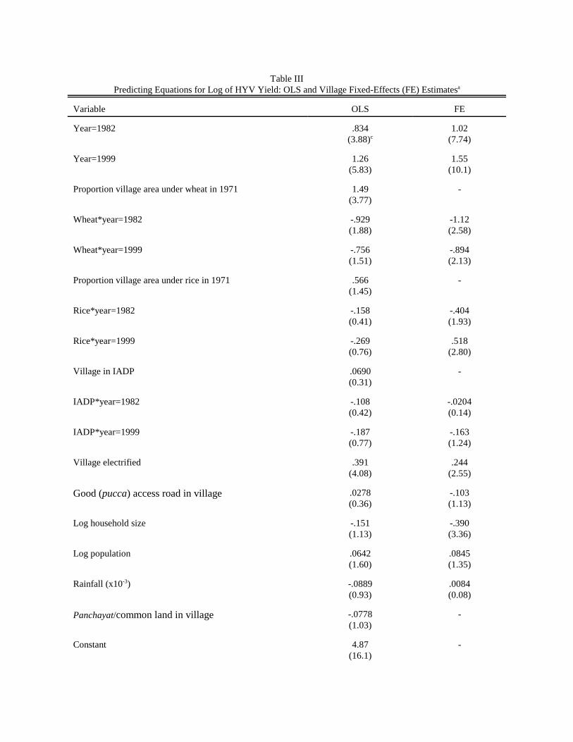
Table IIIPredicting Equations for Log of HYV Yield: OLS and Village Fixed-Effects (FE) Estimatesa

Variable OLS FE

Year=1982 .834(3.88)c

1.02(7.74)

Year=1999 1.26(5.83)

1.55(10.1)

Proportion village area under wheat in 1971 1.49(3.77)

-

Wheat*year=1982 -.929(1.88)

-1.12(2.58)

Wheat*year=1999 -.756(1.51)

-.894(2.13)

Proportion village area under rice in 1971 .566(1.45)

-

Rice*year=1982 -.158(0.41)

-.404(1.93)

Rice*year=1999 -.269(0.76)

.518(2.80)

Village in IADP .0690(0.31)

-

IADP*year=1982 -.108(0.42)

-.0204(0.14)

IADP*year=1999 -.187(0.77)

-.163(1.24)

Village electrified .391(4.08)

.244(2.55)

Good (pucca) access road in village .0278(0.36)

-.103(1.13)

Log household size -.151(1.13)

-.390(3.36)

Log population .0642(1.60)

.0845(1.35)

Rainfall (x10-3) -.0889(0.93)

.0084(0.08)

Panchayat/common land in village -.0778(1.03)

-

Constant 4.87(16.1)

-

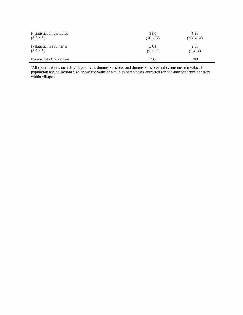
F-statistic, all variables(d.f.,d.f.)

18.0(20,252)

4.26(268,434)

F-statistic, instruments(d.f.,d.f.)

3.04(9,252)

2.63(6,434)

Number of observations 703 703

aAll specifications include village-effects dummy variables and dummy variables indicating missing values forpopulation and household size. cAbsolute value of t-ratio in parentheses corrected for non-independence of errorswithin villages.

Table IVReduced-Form Effects of Agricultural Productivity, Population, and Presence of Rural Infrastructure on

Log Land Prices, Log Wages and Log Household Income: Cross-section OLS, Village Fixed Effects and FE-IV Estimatesa

Variable Log Land Price Log Agricultural Wage Log HH Income Factory in Village

Estimation procedure OLS FE FE-IV OLS FE FE-IV OLS FE FE-IV

OLS FE FE-IV

Log HYV productivity(rupees)b

.423(7.27)c

.265(5.25)

1.52(3.81)

.0515(1.94)c

.0232(0.98)

.0576(0.47)

.0329(1.43)c

.0352(0.88)

.341(1.54)

-.0428(1.76)c

-.0489(2.01)

-.0274(0.20)

Log household size .438(1.70)

.379(2.97)

.764(3.30)

.0460(0.63)

-.131(2.27)

-.118(1.62)

.214(4.66)

.0690(0.83)

.752(5.37)

.0347(0.49)

.0102(0.17)

.0180(0.23)

Log population .182(2.42)

-.210(3.03)

-.283(2.57)

.114(6.06)

-.0872(2.85)

-.0898(2.83)

-.0211(1.14)

.0160(0.36)

.0687(1.58)

.0826(5.27)

.193(6.04)

.192(5.80)

Village electrified .174(1.41)

.0023(0.02)

-.201(1.13)

.155(3.12)

.0317(0.66)

.0223(0.39)

-.0045(0.07)

-.0411(0.55)

.170(2.15)

.0567(1.23)

.166(3.33)

.162(2.82)

Good (pucca) accessroad in village

.255(2.08)

.0056(0.06)

.228(1.32)

.229(3.28)

.113(2.53)

.116(2.53)

.196(3.57)

.246(4.19)

.0124(0.14)

.112(2.53)

.0937(2.00)

.0956(1.98)

Rainfall (mm x 10-3) .0711(0.60)

-.265(2.60)

-.195(1.22)

.0225(0.68)

.0697(1.52)

.0702(1.53)

-.0387(1.99)

.170(2.97)

.0828(1.15)

.0013(0.05)

.0717(1.48)

.0725(1.48)

Panchayat/commonland in village

-.0768(0.53)

- - .0628(1.44)

- - -.0236(0.76)

- - -.0522(1.55)

- -

Number of obs. 697 697 697 703 703 703 484 484 484 726 726 726aAll specifications include year-effects dummy variables and dummy variables indicating missing values for population and household size. bEndogenousvariable in columns 4, 7, 10 and 13. Instruments are: rice-, wheat-growing regions and IADP interacted with year indicator variables. cAbsolute value of t-ratio in parentheses corrected for non-independence of errors within villages.

Table VReduced-Form Effects of Agricultural Productivity, Population, and Presence of Rural Infrastructure

on Forested Area (NDP) and Forest Biomass (NDT):Cross-section OLS, Village Fixed Effects and FE-IV Estimatesa

Variable NDP NDT

Estimation procedure OLS FE FE-IV OLS FE FE-IV

Log HYV productivity(rupees)b

.0534(3.87)c

-.00362(0.22)

-.306(3.25)

.0176(3.59)c

-.00209(0.36)

-.101(3.12)

Log household size -.0199(0.65)

-.0531(1.32)

-.122(2.21)

-.0188(1.74)

-.0192(1.35)

-.0419(2.20)

Log population .0348(3.96)

.0887(4.02)

.0881(3.13)

.0103(3.29)

.0189(2.41)

.0187(1.93)

Village electrified -.0196(0.80)

-.0109(0.31)

.0884(1.63)

-.00410(0.47)

-.00665(0.53)

.0260(1.39)

Good (pucca) accessroad in village

.0535(2.41)

-.0357(1.22)

-.0657(1.71)

.0174(2.21)

-.0167(1.61)

-.0266(2.01)

Rainfall (mm x 10-3) -.00009(0.01)

.0420(1.26)

.0315(0.74)

-.0102(1.75)

-.0296(1.24)

.0181(0.91)

Panchayat/commonland in village

-.0011(0.06)

- - .0012(0.19)

- -

Number of obs. 791 791 791 791 791 791aAll specifications include year-effects dummy variables and dummy variables indicating missing values forpopulation and household size. bEndogenous variable in columns 4 and 7. Instruments are: rice-, wheat-growingregions and IADP interacted with year indicator variables. cAbsolute value of t-ratio in parentheses corrected fornon-independence of errors within villages.

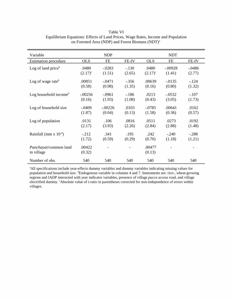
Table VIEquilibrium Equations: Effects of Land Prices, Wage Rates, Income and Population

on Forested Area (NDP) and Forest Biomass (NDT)a

Variable NDP NDTEstimation procedure OLS FE FE-IV OLS FE FE-IV

Log of land priceb .0480(2.17)c

-.0283(1.51)

-.130(2.65)

.0480(2.17)c

-.00928(1.41)

-.0486(2.77)

Log of wage rateb .00851(0.58)

-.0471(0.98)

-.356(1.35)

.00639(0.16)

-.0135(0.80)

-.124(1.32)

Log household incomeb -.00256(0.16)

-.0961(1.93)

-.186(1.08)

.0213(0.43)

-.0532(3.05)

-.107(1.73)

Log of household size -.0409(1.87)

-.00226(0.04)

.0103(0.13)

-.0785(1.58)

.00641(0.36)

.0162(0.57)

Log of population .0131(2.17)

.106(3.93)

.0816(2.26)

.0511(2.84)

.0273(2.88)

.0192(1.48)

Rainfall (mm x 10-4) -.212(1.72)

.341(0.59)

.195(0.29)

.242(0.70)

-.240(1.18)

-.288(1.21)

Panchayat/common landin village

.00422(0.32)

- - .00477(0.13)

- -

Number of obs. 540 540 540 540 540 540aAll specifications include year-effects dummy variables and dummy variables indicating missing values forpopulation and household size. bEndogenous variable in columns 4 and 7. Instruments are: rice-, wheat-growingregions and IADP interacted with year indicator variables, presence of village pucca access road, and villageelectrified dummy. cAbsolute value of t-ratio in parentheses corrected for non-independence of errors withinvillages.

Table VIIVillage Fixed-Effects Estimates: Determinants of Household Fuel Expenditure (1971 Rupees)

Variable

All VillagesVillages with

Commons

Villageswithout

Commons

All Villages

Household size 1.92(4.53)a

1.88(2.75)

1.99(4.10)

1.99(4.11)

Household income .00653(10.6)

.00677(8.02)

.00617(7.36)

.00617(7.38)

Common-land village*householdsize

- - - -.110(0.13)

Common-land village*income - - - .00060(0.51)

Number of households 4,461 2,454 2,007 4,461

Number of villages 259 137 114 259aAbsolute value of t-ratio is in parentheses

Table VIIITest of Equality of the Effects of Household Income, Household and Population Size

on Forested Area (NDP) and Forest Biomass (NDT) Between Common-Land and Non Common-Land Villagesa

Variable NDP NDTEstimation procedure OLS FE FE-IV OLS FE FE-IV

Log of land priceb .0503(2.33)c

-.0241(1.28)

-.0815(2.11)

.0216(2.76)

-.00846(1.28)

-.0295(2.15)

Log of wage rateb .00883(0.22)

-.0629(1.32)

-.108(0.59)

.00960(0.66)

-.0183(1.10)

-.0510(0.79)

Log household incomeb .0317(0.63)

-.0988(1.95)

-.204(1.62)

.00166(0.10)

-.0557(3.14)

-.0987(2.21)

Village common land*logof household incomeb

-.0164(1.87)

-.0152(2.31)

-.0153(1.96)

-.00630(1.85)

-.00610(2.64)

-00630(2.29)

Log of household size .0274(0.24)

.213(2.17)

.246(2.33)

.00509(0.13)

.0859(2.50)

.0996(2.67)

Village common land*logof household size

-.149(1.19)

-.308(2.73)

-.305(2.53)

-.0653(1.45)

-.112(2.82)

-.115(2.69)

Log of population size .0523(2.40)

.106(2.87)

.117(2.87)

.0124(1.73)

.0306(2.37)

.0345(2.38)

Village common land*logof population size

.00056(0.03)

.0126(0.25)

-.0162(0.30)

.00217(0.31)

-.00256(0.15)

-0333(0.69)

Rainfall (mm x 10-4) -.322(0.96)

.460(0.80)

.354(0.58)

-.240(2.04)

.196(0.98)

.222(1.03)

Panchayat/common-landin village

.359(1.34)

- - .137(1.46)

- -

Constant -.752(2.70)

- - -.250(2.61)

- -

Number of obs. 540 540 540 540 540 540aAll specifications include year-effects dummy variables and dummy variables indicating missing values forpopulation and household size. bEndogenous variable in columns 4 and 7. Instruments are: rice-, wheat-growingregions and IADP interacted with year indicator variables and whether or not the village has common land,presence of village pucca access road, and village electrified dummy interacted with whether or not the villagehas common land. cAbsolute value of t-ratio in parentheses corrected for non-independence of errors withinvillages.

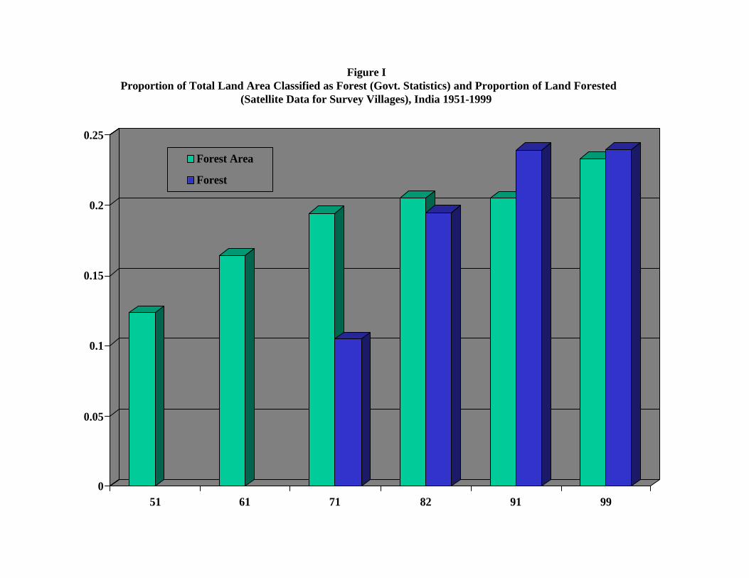
0

0.05

0.1

0.15

0.2

0.25

51 61 71 82 91 99

Forest Area

Forest

Figure IProportion of Total Land Area Classified as Forest (Govt. Statistics) and Proportion of Land Forested

(Satellite Data for Survey Villages), India 1951-1999

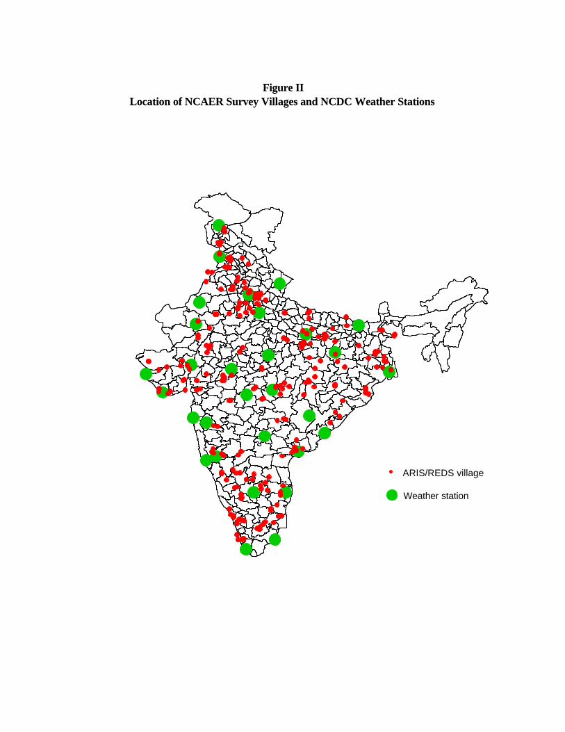
ARIS/REDS village

Weather station

Figure IILocation of NCAER Survey Villages and NCDC Weather Stations