Population HIV-1 Dynamics in Vivo: Applicable Models and

Inferential Tools for Virological Data from AIDS Clinical Trials

Hulin Wu∗

Statistical and Data Analysis Center, Harvard School of Public Health, Frontier Science

& Technology Research Foundation, Inc. 1244 Boylston Street, Suite 303, Chestnut Hill,

Massachusetts 02167, U.S.A.

and

A. Adam Ding

Department of Mathematics, Northeastern University, Boston, Massachusetts 02115,

U.S.A.

SUMMARY

In this paper we introduce a novel application of hierarchical nonlinear mixed-effect models to

HIV dynamics. We show that a simple model with a sum of exponentials can give a good fit

to the observed clinical data of HIV-1 dynamics (HIV-1 RNA copies) after initiation of po-

tent antiviral treatments, and can also be justified by a biological compartment model for the

interaction between HIV and its host cells. This kind of model enjoys both biological inter-

pretability and mathematical simplicity after reparameterization and simplification. A model

simplification procedure is proposed and illustrated through examples. We interpret and justify

various simplified models based on clinical data taken during different phases of viral dynamics

during antiviral treatments. We suggest the hierarchical nonlinear mixed-effect model approach

for parameter estimation and other statistical inferences. In the context of an AIDS clinical

trial involving patients treated with a combination of potent antiviral agents, we show how the

models may be used to draw biologically relevant interpretations from repeated HIV-1 RNA

measurements and demonstrate the potential use of the models in clinical decision-making.

∗ Corresponding author’s email address: wu@sdac.harvard.edu

Key Words: Hierarchical models; HIV infection; Mixed-effect models; Nonlinear regression; Random

effect models; Viral load.

1. Introduction

1.1 Background

The development of assay techniques for quantifying HIV-1 RNA in HIV-1 infected pa-

tients makes it possible to use viral load (HIV-1 RNA copies) as a surrogate marker to

accelerate AIDS clinical trials. Recently some deterministic HIV-1 dynamic models have

been developed to describe the interaction between HIV and its host cells in individual

patients (Perelson, Kirschner and De Boer, 1993; Schenzle, 1994; Kirschner and Perelson,

1995; Kirschner, 1996; Phillips, 1996; De Boer and Boucher, 1996; Nowak and Bangham,

1996). A stochastic model is also proposed by Tan and Wu (1998).

However, most of the models developed by biomathematicians and biologists are too

complicated and contain too many unknown parameters to be used to analyze real clinical

data. Recently several simplified models have been proposed and applied to real virolog-

ical data from clinical trials (Ho et al., 1995; Wei et al., 1995; Perelson et al., 1996 and

1997). These studies of HIV dynamics have led to a new understanding of the pathogen-

esis of HIV infection. However, various assumptions have to be made in order to simplify

these models; some of these assumptions may not be valid in practice. The estimation

methods used in these studies are not efficient and not flexible enough to deal with sparse

data. Although biomathematicians and theoretical biologists have worked on mathemati-

cal dynamic models of HIV since the end of the 1980’s (Merrill, 1987; Anderson and May,

1989; Perelson, 1989), few statisticians have been involved in this effort. We expect that

this paper can stimulate more research in this field among statisticians.

HIV dynamic models provide a global picture of the virus elimination and production

process during antiviral treatments for each individual patient. Thus in evaluating the

efficacy of anti-HIV treatments and understanding HIV infection pathogenesis, it is of

great interest to estimate viral dynamic parameters for the whole population and for each

individual patient in an AIDS clinical trial.

1.2 A Clinical Data Example

In AIDS Clinical Trial Group (ACTG) Protocol 315, fifty-three HIV infected patients

were treated with potent antiviral drugs (ritonavir, 3TC and AZT). Plasma HIV-1 RNA

was repeatedly quantified on Days 2, 7, 10, 14, 21, 28, and Weeks 8, 12, 24 and 48 after

initiation of treatment. The Nucleic Acid Sequence-Based Amplification assay (NASBA)

1

was used to measure plasma HIV-1 RNA. This assay offers a lower limit of detection of

100 RNA copies per ml plasma. We present repeated measurements of viral load from

four of these patients in Figure 1. The viral load in all other patients follow a similar

pattern, i.e., after initiation of antiviral treatment, a fast decay of plasma virus followed by

a slower decay (commonly referred to as two phase decay). The investigators of the study

were interested in the following scientific questions: (1) what is the mechanism behind

the two phases of virus decay? (2) what is the biological meaning of the decay rates of the

two phases? (3) how can we characterize viral dynamics in the patient population and

intra- and inter-subject variations? (4) how can we estimate the decay rates of these two

phases for each individual patient and use this information in making clinical decisions

for individuals? (5) how can we use the results of modeling and estimation in clinical

practice?

Place of Figure 1

The purposes of this paper are, (1) to introduce a viral dynamic model (Section 2.1)

and to simplify it to an estimable function, allowing the mechanism of two-phase viral

decay and its biological meaning to be explained by simple and estimable HIV-1 dynamic

models (Section 2.2); (2) to demonstrate the use of the hierarchical nonlinear mixed-effect

model statistical framework as a basis for estimation of population and individual viral

dynamic parameters (Section 3); and (3) to show how the models may be used to draw

biologically relevant interpretations and aid in clinical decision-making within the context

of the data from ACTG 315 (Section 4).

2. HIV Dynamic Models and Simplifications

2.1 A Model of HIV Dynamics

We propose a mathematical model for HIV dynamics by considering the following cell and

virus compartments: (1) uninfected target cells, such as T cells, macrophages, lymphoid

mononuclear cells (MNCs), and tissue langerhans cells, which are possible targets of

HIV-1 infection; (2) “mysterious” infected cells, cells other than T cells, such as tissue

langerhans cells and microglial cells whose behavior is not completely known; (3) long-

lived infected cells, such as macrophages, that are chronically infected and long-lived; (4)

2

latently infected cells, which contain the provirus but are not producing virus immediately,

and only start to produce virus when activated; (5) productively infected cells, which

are actively producing virus; (6) infectious virus, virus that is functional and capable

of infecting target cells; (7) noninfectious virus, virus that is dysfunctional and cannot

infect target cells. We denote the concentration of the variety of these cells and virus by

T, Tm, Ts, Tl, Tp, VI, and VNI , respectively.

Without the intervention of antiviral treatment, uninfected target cells may either

decrease due to HIV infection or be in an equilibrium state due to balancing between re-

generation and proliferation of uninfected target cells and HIV infection. Some uninfected

target cells (T ) are infected by infectious virus (VI) and may become mysterious infected

cells (Tm), long-lived infected cells (Ts), latently infected cells (Tl) or productively in-

fected cells (Tp) with proportions of αmkVI , αskVI , αlkVI , and αpkVI, respectively, where

αm + αs + αl + αp = 1. Latently infected T cells may be stimulated to become produc-

tively infected cells with a rate of δl. Infected cells, Tm, Ts and Tp, are killed by HIV at

the rates of δm, δs and δp, respectively, after producing an average of N virions per cell

during their lifetimes. Infected cells, Tm, Ts and Tl may also die at the rates of µm, µs and

µl, respectively, without producing virus. We assume that the proportion of noninfectious

virus produced by infected cells is η, without the intervention of protease inhibitor (PI)

antiviral drugs. The elimination rates for infectious virus and noninfectious virus are

assumed to be the same, say c.

We assume that the antiviral therapy consists of one or more protease inhibitor (PI)

drugs and reverse transcriptase inhibitor (RTI) drugs. We model the effect of RTI drugs

by reducing the infection rate from k0 to (1 − γ)k0, where 0 ≤ γ ≤ 1 (Herz, et al., 1996).

Parameter γ reflects the RTI drug efficacy (Bonhoeffer, Coffin, and Nowak, 1997). If

γ = 0, the RTI drugs have no effect; if γ = 1, the RTI drugs are perfect and completely

block the HIV infection. The PI drugs are assumed to be so potent that the production

of infectious virions is almost blocked except for a small fraction. To account for com-

partments where the PI drugs cannot reach and persistent virus that the PI drugs cannot

completely block the production of, we consider an additional virus production term with

a constant (average) rate, P , in the model. If only a small fraction of persistent virus can

escape from the attack of PI drugs, it may be considered as a Poisson process, and can

thus be modeled by a constant production in a deterministic model. Thus, after initiation

3

of combination treatment with PI and RTI drugs, the HIV dynamic model is

ddt

Tm = (1 − γ)αmk0TVI − δmTm − µmTm,

ddt

Ts = (1 − γ)αsk0TVI − δsTs − µsTs,

ddt

Tl = (1 − γ)αlk0TVI − δlTl − µlTl,

ddt

Tp = (1 − γ)αpk0TVI + δlTl − δpTp,

ddt

VI = (1 − η)P − cVI ,

ddt

VNI = ηP + NδmTm + NδsTs + NδpTp − cVNI .

(1)

where αm + αs + αl + αp = 1.

Ideally, it is unlikely that the target cell density T is constant; Perelson et al. (1993)

have represented T by the following nonlinear differential equation:

d

dtT = s + rT T

(

1 −T + Tm + Ts + Tl + Tp

Tmax

)

− k1VIT − µT T (2)

where s is a regeneration rate. The term rT T(

1 − T+Tm+Ts+Tl+Tp

Tmax

)

is a logistic proliferation

rate. The term k1VIT models the rate at which infectious virus infects a target cell, and

µT is the death rate of target cells; see Perelson et al. (1993) for details. Due to the

nonlinearity introduced by (2), the system of differential equations (1) is analytically

intractable. Fortunately, however, the CD4+ T cell count changes much more slowly than

viral load, and the T cell count recovers slightly during the first 2 to 4 weeks of antiviral

treatment and then reaches steady-state rapidly. Thus, a reasonable simplification is to

approximate this recovery process from (2) by T = T0 + Tr(1 − e−rt). This simplification

may not be ideal, but carries the advantage that the system of equations (1) may be

solved analytically; moreover, we have investigated this simplification by simulation for

scenarios similar to that of the ACTG 315 data, and found the approximation to be quite

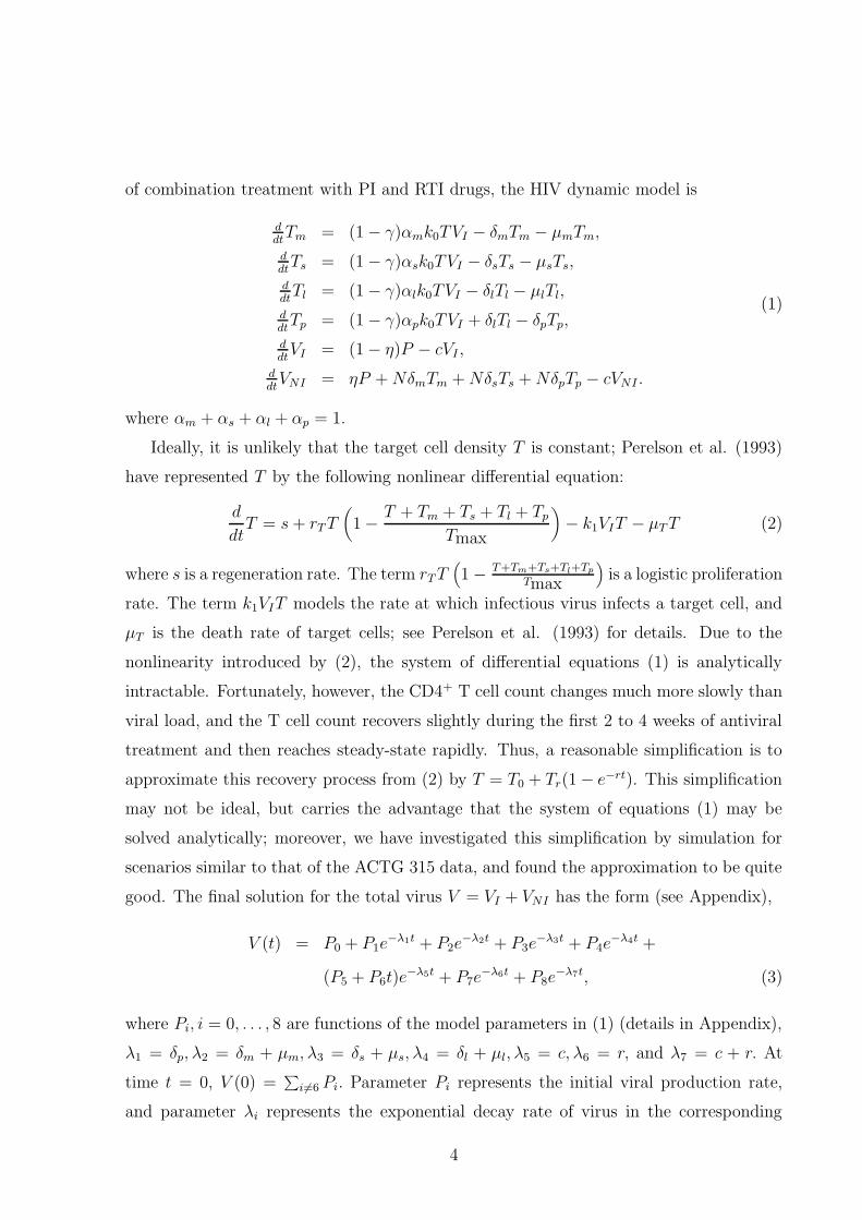
good. The final solution for the total virus V = VI + VNI has the form (see Appendix),

V (t) = P0 + P1e−λ1t + P2e

−λ2t + P3e−λ3t + P4e

−λ4t +

(P5 + P6t)e−λ5t + P7e

−λ6t + P8e−λ7t, (3)

where Pi, i = 0, . . . , 8 are functions of the model parameters in (1) (details in Appendix),

λ1 = δp, λ2 = δm + µm, λ3 = δs + µs, λ4 = δl + µl, λ5 = c, λ6 = r, and λ7 = c + r. At

time t = 0, V (0) =∑

i6=6 Pi. Parameter Pi represents the initial viral production rate,

and parameter λi represents the exponential decay rate of virus in the corresponding

4

compartment. Also notice that, if P in (1) cannot be approximated by a constant due to

dependence on the density of infected cells, the decay rates λ1, ..., λ7 would not be exactly

the elimination rates of infected cells. Instead they would be complicated functions of all

parameters in (1). We shall explore this problem in detail in the future.

As suggested by Herz et al. (1996) and others (Perelson et al., 1996 and 1997; Wu

et al., 1997 and 1998b), several phases of HIV-1 dynamics may exist after initiation of

antiviral treatments. There are several hours of intracellular and pharmacological delay

after the first dose of antiviral drugs; thereafter the viral decay will follow the function (3).

First there is a transition phase reflecting the decay of free virus and productively infected

cells (Perelson et al., 1996; Herz et al., 1996). This is followed by a rapid exponential

decay which mainly reflects the decay of productively infected cells. The decay becomes

slower after several weeks, which may reflect the decay of long-lived infected cells and/or

latently infected cells (Perelson et al., 1997), or may be due to the constant production

P0 discussed in the last section (Wu et al., 1997). We believe that other decay phases

may also exist, but may not be identified due to the limited sensitivity and accuracy of

current HIV-1 RNA assays. We illustrate various phases of HIV-1 dynamics in Figure 2.

Place of Figure 2

2.2 Simplified Models for Clinical Data

There are some difficulties in applying this model to real data analysis. First, we have

to estimate the intracellular and pharmacological delay as shown in Figure 2, which re-

quires frequent measurement data on viral load and pharmacokinetics in the first several

hours after initiation of antiviral treatment (Herz et al., 1996; Perelson et al., 1996). This

kind of data is very expensive and rarely available in clinical trials unless the trial is

specifically designed to gather it. However, we can see from (3) that, if there is an intra-

cellular/pharmacological delay period of td, the solution is the same with the parameters

Pi replaced by Pieλitd . Therefore we can ignore the delay and still correctly estimate the

parameters λi, which medical investigators are mostly interested in due to their biological

correlation with treatment efficacy and turnover rates of virus and infected cells. The

estimate of the Pi’s may be biased, but not very seriously, since td is only several hours

(Perelson et al., 1996).

5

Secondly, formula (3) is still too complicated and contains too many parameters. In

theory, if very accurate measurements are available over a very long time, all parame-

ters in the model (3) can be identified (Godfrey, 1983). However, due to measurement

noise, poor assay sensitivity, and limited sampling schedules, only a small number of

exponentials can be realistically fitted to the repeated measurements of total virus. If

some of the exponential decay rates, λ1i, . . . , λqi, are not well separated, it may also cause

unidentifiability problems.

Therefore we propose a procedure to simplify model (3) in order to estimate the

important and clinically interesting parameters based on measurements of total viral

load, V = VI +VNI . This procedure is motivated by the exponential curve peeling method

(Anderson, 1983; Van Liew, 1967) which fits a multiple-exponential curve piecewise in a

backward order. However, our method involves approximating the multiple-exponential

curve forwards. The basic idea is illustrated in the following discussion.

First we consider that HIV-1 RNA data are obtained frequently from initiation of

antiviral treatment up to the first rapid decay phase (Figure 2). In this case, the data

only allow us to model the productively infected cells and virus compartments (Perelson

et al., 1996; Wu, Ding and DeGruttola, 1998a). However, unlike Perelson et al. (1996)

and Wu et al. (1998a), in which the other infected cell compartments such as Tm, Ts, and

Tl are simply ignored, here we propose to approximate these ignored compartments by a

constant virus production. Since the ignored infected cells have a relatively long half-life,

the virus decay due to these compartments will be slow in a short time period, and remain

approximately constant. Therefore model (1) can be simplified as

ddt

Tp = k∗TVI − δpTp,

ddt

VI = (1 − η)P − cVI ,

ddt

VNI = ηP + P ∗ + NδpTp − cVNI ,

(4)

where P ∗ accounts for virus production from the ignored compartments, Tm, Ts, and Tl,

and T can also be assumed as a constant for the short period. Then an analytic solution

for (4) is

V (t) = P0 + P1e−δpt + (P2 + P3t)e

−ct. (5)

Note that the number of parameters to be estimated is reduced to six. Following Perel-

son, et al. (1996, 1997), the number of parameters may be further reduced by assuming a

6

quasi-steady state condition before treatment; however, this condition may not always be

realistic in actual clinical trials (Perelson et al., 1997). Moreover, simplified models using

steady-state conditions lead to serious nonlinearity in parameters, which causes difficul-

ties and inefficiency in parameter estimation and other statistical inferences (Ratkowsky,

1983).

When the viral load data are available for a longer period, more infected cell compart-

ments may be considered (Perelson et al. 1997; Wu et al., 1997 and 1998b). However,

due to the limited accuracy and sensitivity of current HIV-1 RNA assays, perhaps only

one more compartment can be realistically identified; the virus production from other

compartments may again be approximated by a constant P ∗. Simplifying in a manner

similar to that used in above, we can obtain the total virus load in the form

V (t) = P0 + P1e−δpt + P2e

−λt + (P3 + P4t)e−ct, (6)

where λ is a possibly confounded clearance rate of long-lived and latently infected cells

(Perelson et al., 1997; Wu et al., 1998b). However, we also recall that the clearance of

free virus has been estimated to be very rapid (less than 6 hours of half-life, see Perelson

et al. 1996). Hence the term due to the clearance of free virus, (P3 + P4t)e−ct in model

(6), will be negligible compared to other terms due to the clearance of infected cells after

a few days of treatment. Thus the model can be further simplified as

V (t) = P0 + P1e−δpt + P2e

−λt, for t ≥ tc, (7)

where tc is the time required for the term (P3 + P4t)e−ct to become negligible.

In general, if viral dynamics data for only a segment of the treatment time are available

from a clinical trial, we may simplify the viral dynamic model by considering the following:

(i) we may ignore some terms associated with the faster decays (e.g. free virus and

productively infected cells) as in the above examples, if they are negligible in the modeling

time period based on results from similar studies or published literature; (ii) we may

approximate slower decays (e.g. long-lived infected cells or mysterious infected cells) by

constants if they are slow enough in the modeling time period; (iii) if the sensitivity and

accuracy of HIV-1 RNA assays do not allow us to accurately estimate all compartment

terms, it is better to neglect some compartments or replace them by simpler terms such

as a constant. Sometimes we may intentionally use only a segment of the viral dynamic

7

data even when we have the complete data, since this may help to simplify the model,

and thus some important parameters can be more efficiently estimated (Wu et al., 1997);

(iv) Statistical model selection criteria such as AIC or BIC may be used to simplify the

models.

The single exponential models (Ho et al. 1995; Wei et al. 1995) and bi-exponential

models (Wei et al. 1995 and Wu et al. 1998b) are special cases of our model (7) arrived at

by further ignoring some slowly decaying compartments and the constant term. But these

oversimplified models sometimes may yield misleading results (Wu et al., 1997). Thus we

recommend using a constant term to approximate the slowly decaying compartments un-

less some hard evidence or statistical model selection methods show that it is unnecessary.

3. Hierarchical Nonlinear Mixed-Effect Model Approach

The structure of data such as those from ACTG 315 is that of repeated viral load mea-

surements on each of a number of subjects. Because the viral dynamic process described

by the models in Section 2 takes place within a given subject, and the process may differ

among subjects, a natural statistical framework is that of the hierarchical nonlinear mixed

effect model (Davidian and Giltinan, 1995). Specifically, we consider the following general

model:

Stage 1. Intra-patient variation in viral load measurement:

yij = log(V (tij, βi)) + eij, ei|βi ∼ (0, Ri(βi, ξ)), (8)

where yij is the log-transform of the total viral load measurement for the ith patient

and at the jth time point tij, i = 1, . . . , m; j = 1, . . . , ni. The log-transformation

of raw data is used to stabilize the variance (it is also more normally distributed).

Model (3) can be re-written as

V (tij, βi) =k

∑

`=0

eθ`i−λ`itij , (9)

where the θ’s are the log-transformations of the P ’s, the coefficients of exponentials

in the last section. With the log-transformation, the new parameters, θ`i = log(P`i),

are of similar scale as the λ’s, the exponential decay rates. Denote the dynamic

parameters for the ith patient by βi = [θ0i, . . . , θki, λ1i, . . . , λqi]′. The within-patient

8

random error ei = [ei1, . . . , eini]′ has a zero mean and covariance matrix Ri condi-

tional on βi.

Stage 2, Inter-patient variation:

θ0i = θ0 + b0i, . . . θki = θk + bki, (10)

λ1i = λ1 + b(k+1)i, . . . λqi = λq + b(k+q)i. (11)

Population parameters are β = [θ0, . . . , θk, λ1, . . . , λq]′. Random effects are

bi = [b0i, . . . , b(k+q)i]′ ∼ (0, D).

For the real data analysis in the next section, we used a diagonal variance-covariance

matrix Ri (uncorrelated within-patient measurements). A more complicated structure

may be considered in the future. All the dynamic models we fitted to the ACTG 315

data in the next section were carried out within this statistical framework. The real data

support that the θ’s and λ’s are likely to be normally distributed. The log-transformed

parameter, θ`i = log(P`i), can also ensure the positivity of the parameters and improve

the estimation stability.

A number of inferential procedures are available for fitting hierarchical nonlinear mixed

effects models, see Davidian and Giltinan (1995) for an overview. These methods allow

estimation of population parameters β and D as well as prediction of individual para-

meters βi via empirical Bayes techniques. Because the data from HIV dynamic studies

may be sparse for some patients, we favor methods based on linearization of the model in

the random effects. A number of software implementations are in widespread use (Roe,

1997); for analysis of the data from ACTG 315, we used the Splus function NLME, which

implements the method of Lindstrom and Bates (1990). For such procedures, model se-

lection criteria such as Akaike’s (AIC) and Schwarz’s Bayesian (BIC) information criteria

have been advocated for comparison of competing models; for the particular structure of

viral dynamic models, Wu et al. (1998a) found BIC to be more reliable.

4. Analysis of ACTG 315 Data

The modeling and inferential methods of the previous sections were applied to the data

from ACTG 315. Of the 53 patients, 7 either dropped out from the study or showed

9

profiles that did not correspond to the pattern of the rest of the patients, exhibiting no

response to the antiviral drugs due to poor absorption of the drugs, noncompliance, drug

resistance, or other unknown reasons. The remaining subjects had between 3 and 9 viral

load measurements; data from four representative patients are shown in Figure 1. It

is worth noting that the HIV-1 RNA assay has a limit of detection of 100 copies. For

patients with measurements below detectable level, we imputed the values to be 50 (=1.7

in log10 scale). Since viral rebound due to drug resistance and noncompliance is not taken

into account in our models, the data after viral rebound are excluded from our analysis.

Considering that, after a long time period, the data are likely to be contaminated and

influenced by factors such as drug resistance, noncompliance, and assay detection limits,

and model assumptions may not hold, we stopped using the data after 12 weeks.

As proposed in Section 2, since the viral load data are available only after 2 days

following the initiation of treatment, the exponential decay term related to the clearance

of free virus, e−ct, can be ignored. Based on the estimate c = 3 day−1 in Perelson et al.

1996, the terms containing e−ct account for less than 1% of the total viral load after 2

days and account for less than 0.0001% of the total viral load after 7 days.

We considered the following two simplified models based on the suggestions in Sec-

tion 2, since both models can capture two observed phases of virus decay.

V (t) = P0 + P1e−δpt, (12)

V (t) = P1e−δpt + P2e

−λlt. (13)

The AIC and BIC were used to compare the two models. On the basis of AIC and

BIC values (see Table 1), Model (13) is preferred. Attempts to fit more complex models

were not fruitful, most likely because the data are not rich enough to identify more

compartments. From the fit of (13), estimates of individual profiles based on empirical

Bayes methods, available in the NLME software, are shown for 4 patients in Figure 1; the

model seems to provide a good fit. A summary of estimation results from both models

is given in Table 1. Standard diagnostic plots of observed vs. fitted values based on the

population estimate of β, residuals vs. fitted values based on this estimate, and residuals

based on empirical Bayes estimates of the βi for each patient (Pinheiro and Bates, 1995)

revealed no anomalies indicating gross lack-of-fit.

10

Place of Table 1

The results from the preferred model (Table 1) are very important for understand-

ing the biological mechanism and pathogenesis of HIV-1 infection. The individual esti-

mates of the viral dynamic parameters can be used for clinical decisions in the treat-

ment of individual patients. First, the population estimates of the two decay rates,

δ̂p = 0.442 ± 0.029, λ̂l = 0.032 ± 0.003, represent the turnover rates of productively

infected cells and long-lived and/or latently infected cells, respectively. The correspond-

ing half-lives [log(2)/δp and log(2)/λl] of these two virus compartments can be calculated

as 1.57 ± 0.103 days and 21.66 ± 2.03 days respectively. These estimated life-times of

infected cells are believed to be shorter than those of normal uninfected cells, although

some debates still exist. Undoubtedly, these estimation results would help immunologists

and virologists to understand the cell kinetics and the interaction mechanisms of HIV-1

and its target cells.

Second, the ratio, P2/(P1+P2) gives an approximate estimate of the proportion of virus

produced by long-lived and/or latently infected cells in the total virus pool. Our estimate

is 1.1%, which indicates that most of the virus is produced by productively infected

cells, and only a small proportion is produced by long-lived and/or latently infected cells.

Thus antiviral therapies should mainly target the productively infected cells, although

the compartment of long-lived/latently infected cells cannot be ignored.

Third, the individual estimates of the decay rates show that the interpatient varia-

tions are large. The estimates of δp range from 0.17 to 0.64, with an estimated CV of

31% (the corresponding half-life ranges from 1 day to 4 days). The estimates of λl range

from 0.0014 to 0.0534, with an estimated CV of 47% (the corresponding half-life ranges

from 13 days to 483 days). The large interpatient differences indicate that each individual

patient should be treated differently in clinical decisions. For example, the eradication

times for the two compartments, productively infected cells and long-lived and/or latently

infected cells, can be approximated by log P1/δp and log P2/λl. The ranges of estimates of

the eradication time for these two compartments are (14, 71) days and (158, 2688) days.

If the virus is eradicated, patients may stop taking expensive and toxic antiviral drugs.

The estimates of eradication time based on our models and methods give an estimate

for minimum treatment time. This information, combined with other information such

11

as the presence of virus in other reservoirs, may assist clinicians to make decisions and

predictions regarding when to stop treatment. More medical discussion of these findings

can be found in Wu et al. (1998b).

5. Summary and Discussion

In this paper we presented a model for HIV-1 dynamics in vivo, in which we considered

both RTI and PI antiviral drug effects and all the possible infected cell and virus compart-

ments. In order to apply this model to clinical trials, we proposed a procedure to simplify

the model for HIV-1 RNA data in different phases of virological response. Without mak-

ing an assumption of steady-state before treatment, we reduced the model to applicable

models for clinical data by reparameterization and reasonable approximation. We fitted

this model to clinical data within the hierarchical nonlinear mixed effects framework. We

are currently developing SAS macros and Splus functions for fitting HIV dynamic models

using these methods.

Note that many mathematical functions such as polynomial functions, some power

functions (Ratkowsky, 1990) or piecewise linear functions may fit the viral dynamic tra-

jectory equally well or even better. Statisticians usually select a model for their data

based on the convenience and goodness-of-fit to the data. However, without a biological

interpretation and justification, a mathematical model may not be useful. We believe that

a good model should have the following features: (i) good fit to the observed data; (ii)

reasonable biological interpretation; (iii) conceptual and computational simplicity; (iv)

applicability to low-quality and less frequent clinical data; (v) convenience for statistical

inferences and interpretation; (vi) lower costs economically and computationally. The

simplified models for HIV-1 dynamics proposed in this paper enjoy all these features.

Although biological compartment models are sometimes considered complex, the models

proposed in this paper can also be treated as simple statistical models to trace the trajec-

tory of viral load. Then these models can still be used for prediction or other purposes,

but their biological interpretation may not be valid.

ACKNOWLEDGMENT

This work was partially supported by NIAID/NIH grants No. R29 AI43220 and No. U01

AI38855. We thank Drs. Daniel Kuritzkes and Michael Lederman for discussions on viro-

12

logical issues, the team of AIDS Clinical Trial Group Protocol 315 for allowing us to use

the HIV-1 RNA data from their study to illustrate the methodology, and Professor Victor

DeGruttola, the editor, the associate editor and the referee for their thorough reading of

and insightful comments and suggestions on an earlier version of this paper.

REFERENCES

Anderson, D.H. (1983). Compartmental Modeling and Tracer Kinetics. Lecture Notes

in Biomathematics, Springer-Verlag, Berlin.

Anderson, R.M. and May, R.M. (1989). Complex dynamical behavior in the inter-

action between HIV and the immune system. In Cell to Cell Signaling: From

Experiments to Theoretical Models, A. Goldbeter, Ed., Academic, New York.

Bonhoeffer, S., Coffin, J.M. and Nowak, M.A. (1997). Human Immunodeficiency Virus

drug therapy and virus load. Journal of Virology 71, 3275-3278.

Davidian, M. and Giltinan, D.M. (1995). Nonlinear Models for Repeated Measurement

Data. Chapman & Hall, New York.

De Boer, R.J. and Boucher, C.A.B. (1996). Anti-CD4 therapy for AIDS suggested

by mathematical models. Proceedings of the Royal Society of London- Series B:

Biological Sciences 263 (1372), 899-905.

Godfrey, K. (1983). Compartmental Models and Their Application. Academic Press,

London.

Herz, A.V.M., Bonhoeffer, S., Anderson, R.M., May, R.M., and Nowak, M.A. (1996).

Viral dynamics in vivo: Limitations on estimates of intracellular delay and virus

decay. Proc. Natl. Acad. Sci. USA 93, 7247-7251.

Ho, D.D., Neumann, A.U., Perelson, A.S., Chen, W., Leonard, J.M., and Markowitz,

M. (1995). Rapid turnover of plasma virions and CD4 lymphocytes in HIV-1

infection. Nature 373, 123-126.

Kirschner, D.E. (1996). Using mathematics to understand HIV immune dynamics,

Notices of the AMS 43, 191-202.

Kirschner, D.E. and Perelson, A.S. (1995). A model for the immune system response to

HIV: AZT treatment studies, in Mathematical Population Dynamics: Analysis

13

of Heterogeneity, Vol.1, Theory of Epidemics, O. Arino, D. Axelrod, M. Kimmel,

and M. Langlais, Eds., 295-310.

Lindstrom, M.J. and Bates, D.M. (1990). Nonlinear mixed effects models for repeated

measures data. Biometrics 46, 673-687.

Merrill, S. (1987). AIDS: background and the dynamics of the decline of immunocom-

petence. In Theoretical Immunology, Part 2, A.S. Perelson, Ed., Addison-Wesley,

Redwood City, Calif.

Nowak, M.A. and Bangham, C.R.M. (1996). Population dynamics of immune re-

sponses to persistent viruses. Science 272, 74-79.

Perelson, A.S. (1989). Modeling the interaction of the immune system with HIV. in

Mathematical and Statistical Approaches to AIDS Epidemiology (Lect. Notes

Biomath., Vol. 83), C. Castillo-Chavez, Ed., Springer-Verlag, New York.

Perelson, A.S., Neumann, A.U., Markowitz, M., Leonard, J.M., and Ho, D.D. (1996).

HIV-1 dynamics in vivo: virion clearance rate, infected cell life-span, and viral

generation time. Science 271, 1582-1586.

Perelson, A.S., Essunger, P., Cao, Y., Vesanen, M., Hurley, A., Saksela, K., Markowitz,

M., and Ho, D.D. (1997). Decay characteristics of HIV-1-infected compartments

during combination therapy. Nature 387, 188-191.

Perelson, A.S., Kirschner, D.E. and Boer R.D. (1993). Dynamics of HIV infection of

CD4+ T cells. Mathematical Biosciences 114, 81-125.

Phillips, A.N. (1996). Reduction of HIV concentration during acute infection: inde-

pendence from a specific immune response, Science 271, 497-499.

Pinheiro, J.C. and Bates, D.M. (1995). Mixed-Effects Models Methods and Classes

for S and Splus, downloaded from “ftp://ftp.stat.wisc.edu/src/NLME/Unix”.

Ratkowsky, D.A. (1983). Nonlinear Regression Modeling, A Unified Practical Ap-

proach. Marcel Dekker, Inc., New York.

Ratkowsky, D.A. (1990). Handbook of Nonlinear Regression Models. Marcel Dekker,

Inc., New York.

Roe, D.J. (1997). Comparison of population pharmacokinetic modeling methods using

14

simulated data: Results from the population modeling workgroup. Statistics in

Medicine 16, 1241-1262.

Schenzle D. (1994). A model for AIDS pathogenesis, Statistics in Medicine 13, 2067-

2079.

Tan, W.Y. and Wu, H. (1998). Stochastic modeling of the dynamics of CD4+ T cell

infection by HIV and some Monte Carlo studies. Mathematical Biosciences 147,

173-205.

Van Liew, H.D. (1967). Method of exponential peeling. Journal of Theoretical Biology

16, 43-53.

Wei, X., Ghosh, S.K., Taylor, M.E., Johnson, V.A., Emini, E.A., Deutsch, P., Lifson,

J.D., Bonhoeffer, S., Nowak, M.A., Hahn, B.H., Saag, M.S., and Shaw, G.M.

(1995). Viral dynamics in human immunodeficiency virus type 1 infection. Na-

ture 373, 117-122.

Wu, H., Ding, A.A., and DeGruttola, V. (1998a). Estimation of HIV Dynamic Para-

meters. Statistics in Medicine, in press.

Wu, H.,Kuritzkes, D.R., Clair, M.S., Kessler, H., Connick, E., Landay, A., Heath-

Chiozzi, M., Rousseau, F., Fox, L., Spritzler, J., Leonard, J.M., McClernon,

D.R., and Lederman, M.M. (1997). Interpatient variation of viral dynamics

in HIV-1 infection: Modeling results of AIDS Clinical Trials Group Protocol

315. The First International Workshop on HIV Drug Resistance, Treatment

Strategies and Eradication, Antiviral Therapy, Abstract 99, 66-67.

Wu, H., Kuritzkes, D.R., Clair, M.S., Spear, G., Connick, E., Landay, A., and Leder-

man, M.M. (1998b). Characterizing individual and population viral dynamics

in HIV-1-infected patients with potent antiretroviral therapy: correlations with

host-specific factors and virological endpoints. The 12th World AIDS Confer-

ence. Geneva, Switzerland, June 1998.

APPENDIX

Solutions of the Full Dynamic Model for Antiviral Treatment with Combina-

tion of PI and RTI Drugs

15

From (1), the solution for VI is straightforward by integration,

VI(t) = (1 − η)P/c + [VI(0) − (1 − η)P/c]e−ct.

Plug the above result to equations for Tm, Ts and Tl and using T = T0 + Tr(1 − e−rt) we

easily obtain the following solutions by integration and some algebra.

Tm(t) = bm0 + bm1e−λmt + bm5e

−ct + bm7e−rt + bm8e

−(c+r)t

Ts(t) = bs0 + bs2e−λst + bs5e

−ct + bs7e−rt + bs8e

−(c+r)t

Tl(t) = bl0 + bl3e−λlt + bl5e

−ct + bl7e−rt + bl8e

−(c+r)t,

where

bm0 = (1 − γ)αmk0(T0 + Tr)(1 − η)P/(cλm)

bm1 = Tm(0) − bm0 − bm5 − bm7 − bm8

bm5 = (1 − γ)αmk0(T0 + Tr)[VI(0)c − (1 − η)P ]/[c(λm − c)]

bm7 = −(1 − γ)αmk0Tr(1 − η)P/[c(λm − r)]

bm8 = −(1 − γ)αmk0Tr[VI(0)c − (1 − η)P ]/[c(λm − c − r)].

And bsi and bli, i = 0, 5, 7, 8 have the same expressions as bmi’s with αm and λm replaced

by αs, λs, αl and λl accordingly, and

bs2 = Ts(0) − bs0 − bs5 − bs7 − bs8

bl3 = Tl(0) − bl0 − bl5 − bl7 − bl8

Then the solution for Tp is, (by plug the solution of Tl into equation (1))

Tp(t) = bp0 + bp3e−λlt + bp4e

−δpt + bp5e−ct + bp7e

−rt + bp8e−(c+r)t

where bp4 = Tp(0) − bp0 − bp3 − bp5 − bp7 − bp8 and

bp0 = [(1 − γ)αpk0(T0 + Tr)(1 − η)P/c + δlbl0]/δp

bp3 = δlbl3/(δp − λl)

bp5 = [(1 − γ)αpk0(T0 + Tr)(VI(0) − (1 − η)P/c) + δlbl5]/(δp − c)

bp7 = [−(1 − γ)αpk0Tr(1 − η)P/c + δlbl7]/(δp − r)

bp8 = [−(1 − γ)αpk0Tr(VI(0) − (1 − η)P/c) + δlbl8]/(δp − c − r).

Plug all the above solutions into equation (1), we are left with a first-order linear differ-

ential equation for VNI . Hence the solution for VNI is

VNI(t) = P ∗0 + P1e

−λmt + P2e−λst + P3e

−λlt + P4e−δpt

P ∗5 e−ct + P6te

−ct + P7e−rt + P8e

−(c+r)t.

16

where P ∗5 = VNI(0) − P ∗

0 − P1 − P2 − P3 − P4 − P7 − P8 and

P ∗0 = (Nδpbp0 + Nδmbm0 + Nδsbs0 + ηP )/c

P1 = Nδmbm1/(c − λm) P2 = Nδsbs2/(c − λs)

P3 = Nδpbp3/(c − λl) P4 = Nδpbp4/(c − δp)

P6 = Nδpbp5 + Nδmbm5 + Nδsbs5

P7 = N(δpbp7 + δmbm7 + δsbs7)/(c − r) P8 = −N(δpbp8 + δmbm8 + δsbs8)/r

Finally we get the total virus load, V (t) = VI(t) + VNI(t), as

V (t) = P0 + P1e−λmt + P2e

−λst + P3e−λlt + P4e

−δpt

+(P5 + P6t)e−ct + P7e

−rt + P8e−(c+r)t.

where P0 = P ∗0 + (1 − η)P/c and P5 = V (0) − P0 − P1 − P2 − P3 − P4 − P7 − P8.

17

Table 1: Estimation Results (SE represents the standard error)

Effects Parameters Model (12) Model (13)

δp (SE) 0.216 (0.011) 0.442 (0.029)

Fixed λl (SE) - 0.032 (0.003)

Effects log P0 (SE) 11.023 (0.222) -

log P1 (SE) 5.530 (0.192) 12.142 (0.240)

log P2 (SE) - 7.624 (0.252)

Standard δp 0.035 0.137

Deviation λl - 0.015

of log P0 1.284 -

Random log P1 1.100 1.397

Effects log P2 - 1.545

σ 0.381 0.267

Loglikelihood -230.469 -162.151

AIC 480.938 354.302

BIC 518.838 411.013

Time (day)

Log1

0 R

NA

cop

ies/

ml

0 20 40 60 80

23

45

6

oo

o oo

oo

(a) Subject 1

Time (day)

Log1

0 R

NA

cop

ies/

ml

0 20 40 60 80

2.0

2.5

3.0

3.5

4.0

4.5

5.0

oo

o

o

o

oo

o

(b) Subject 2

Time (day)

Log1

0 R

NA

cop

ies/

ml

0 20 40 60 80

23

45

6

oo

oo

o o

oo

(c) Subject 3

Time (day)

Log1

0 R

NA

cop

ies/

ml

0 20 40 60 80

23

45

67

o

oo

oo

o

o o

(d) Subject 4

Figure 1: Plasma HIV-1 RNA copies (log10 scale) and fitted curves of simplified model,

V (t) = P1e−δpt + P2e

−λlt for 4 patients, where the circles are the observed values, and the

solid lines are fits of the four individual profiles based on empirical Bayes estimates of

individual-specific model parameters.

time

log

( pl

asm

a vi

rus

load

)

|

start of treatment

|

intracellular and pharmacological

delay

/

transition phase: reflecting decay of free virus and

productively infected cells

/

rapid decay phase: reflecting decay of productively, long-lived and/or latently infected cells

|

slow decay phase: reflecting decay of long-lived and/or latently infected cells

and other residual infected cells

levelling off to steady state: reflecting residual virus production and virus

replenishment from other reservoirs

Figure 2: Illustration of the different phases of plasma viral dynamics following antiviral

drug treatment. If the data on the transition phase and rapid decay phase are available,

the suggested model is V (t) = P0 + P1e−δpt + (P2 + P3t)e

−ct. If the data on the rapid

decay phase and slow decay phase are available, the suggested model is V (t) = P0 +

P1e−δpt + P2e

−λt. If the data on the slow decay phase and leveling off phase are available,

the suggested model is V (t) = P0 + P2e−λt. The suggested models should be refined by

the model selection procedure. In the phase of intracellular and pharmacological delay,

the dotted line denotes non-steady-state case before treatment.