polynomial factor models: non-iterative estimation via ... · pdf filepolynomial factor...
TRANSCRIPT

Polynomial factor models: non-iterative estimation viamethod-of-moments
Florian Schuberth12 Rebecca Buchner3 Karin Schermelleh-Engel3
Theo K. Dijkstra4
1University of Wurzburg, Germany
2University of Twente, The Netherlands
3University of Frankfurt, Germany
4Unversity of Groningen, The Netherlands
March 17, 2017
SEM Meeting, Ghent
MoMpoly March 17, 2017 1 / 25
Overview
1 Polynomial factor model
2 Non-iterative method-of-moments
3 Monte Carlo simulation
4 MoMpoly package
MoMpoly March 17, 2017 2 / 25
Structural model
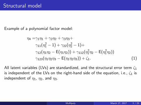
Example of a polynomial factor model:
η4 =γ1η1 + γ2η2 + γ3η3+
γ11(η21 − 1) + γ22(η22 − 1)+
γ12(η1η2 − E(η1η2)) + γ112(η21η2 − E(η21η2))
γ123(η1η2η3 − E(η1η2η3)) + ζ1. (1)
All latent variables (LVs) are standardized, and the structural error term ζ1is independent of the LVs on the right-hand side of the equation, i.e., ζ1 isindependent of η1, η2, and η3.
MoMpoly March 17, 2017 3 / 25
Measurement model
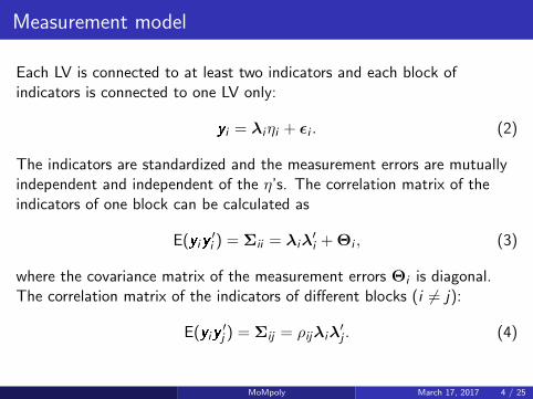
Each LV is connected to at least two indicators and each block ofindicators is connected to one LV only:
yi = λiηi + εi . (2)
The indicators are standardized and the measurement errors are mutuallyindependent and independent of the η’s. The correlation matrix of theindicators of one block can be calculated as
E(yiy′i ) = Σii = λiλ
′i + Θi , (3)
where the covariance matrix of the measurement errors Θi is diagonal.The correlation matrix of the indicators of different blocks (i 6= j):
E(yiy′j ) = Σij = ρijλiλ
′j . (4)
MoMpoly March 17, 2017 4 / 25
Proxies and weights
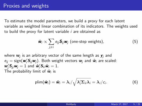
To estimate the model parameters, we build a proxy for each latentvariable as weighted linear combination of its indicators. The weights usedto build the proxy for latent variable i are obtained as
wi ∝∑j 6=i
eijSijwj (one-step weights), (5)
where wj is an arbitrary vector of the same length as yj andeij = sign(w ′
i Sijwj). Both weight vectors wj and wi are scaled:w ′
jSjjwj = 1 and w ′i Sii wi = 1.
The probability limit of wi is
plim(wi ) = wi = λi/√
λ′iΣiiλi = λi/ci . (6)
MoMpoly March 17, 2017 5 / 25
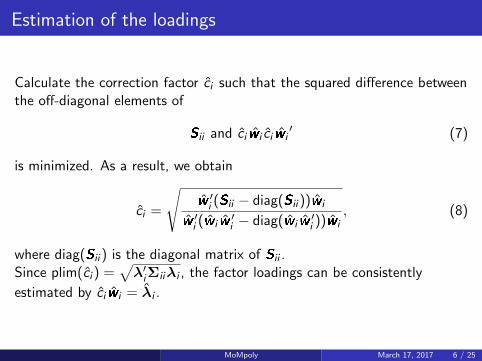
Estimation of the loadings
Calculate the correction factor ci such that the squared difference betweenthe off-diagonal elements of
Sii and ci wi ci wi′ (7)
is minimized. As a result, we obtain
ci =
√w ′
i (Sii − diag(Sii ))wi
w ′i (wi w
′i − diag(wi w
′i ))wi
, (8)
where diag(Sii ) is the diagonal matrix of Sii .Since plim(ci ) =
√λ′iΣiiλi , the factor loadings can be consistently
estimated by ci wi = λi .
MoMpoly March 17, 2017 6 / 25
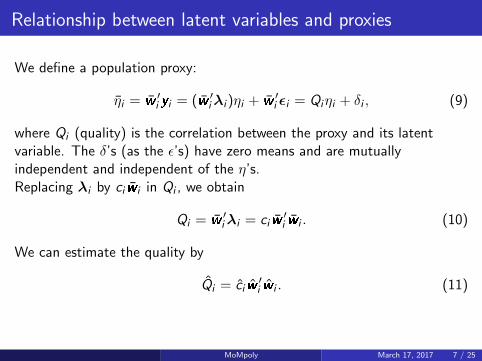
Relationship between latent variables and proxies
We define a population proxy:
ηi = w ′i yi = (w ′
iλi )ηi + w ′i εi = Qiηi + δi , (9)
where Qi (quality) is the correlation between the proxy and its latentvariable. The δ’s (as the ε’s) have zero means and are mutuallyindependent and independent of the η’s.Replacing λi by ci wi in Qi , we obtain
Qi = w ′iλi = ci w
′i wi . (10)
We can estimate the quality by
Qi = ci w′i wi . (11)
MoMpoly March 17, 2017 7 / 25

Relationship between latent variables and proxies
Relationship between the correlation of the proxies and the correlationbetween the latent variables:
E(ηi ηj) = QiQjE(ηiηj), (12)
where E(ηi ηj) is estimated by the sample covariance between the proxies iand j .Using PLS weights, this is already known and published:
for linear models by [Dijkstra, T.K. & Henseler, J., 2015], and
for polynomial models by[Dijkstra, T. K. & Schermelleh-Engel, K., 2014].
New:
the use of one-step weights
implementation in the MoMpoly package in R[Schuberth, F. & Dijkstra, T. K.& Schamberger, T., 2017]
MoMpoly March 17, 2017 8 / 25
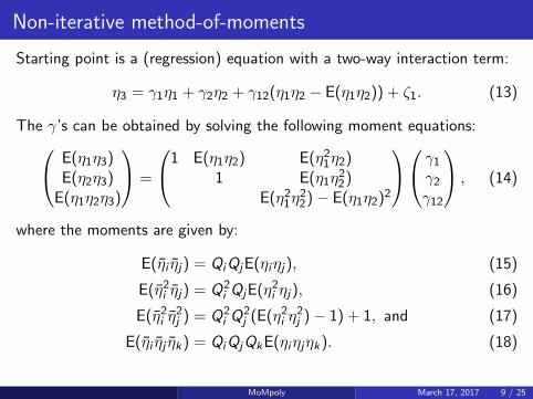
Non-iterative method-of-moments
Starting point is a (regression) equation with a two-way interaction term:
η3 = γ1η1 + γ2η2 + γ12(η1η2 − E(η1η2)) + ζ1. (13)
The γ’s can be obtained by solving the following moment equations: E(η1η3)E(η2η3)
E(η1η2η3)
=
1 E(η1η2) E(η21η2)1 E(η1η
22)
E(η21η22)− E(η1η2)2
γ1γ2γ12
, (14)
where the moments are given by:
E(ηi ηj) = QiQjE(ηiηj), (15)
E(η2i ηj) = Q2i QjE(η2i ηj), (16)
E(η2i η2j ) = Q2
i Q2j (E(η2i η
2j )− 1) + 1, and (17)
E(ηi ηj ηk) = QiQjQkE(ηiηjηk). (18)
MoMpoly March 17, 2017 9 / 25
Non-iterative method-of-moments
So far, no distributional assumptions are necessary. We only assumethat
the moments exist,
the measurement errors are mutually independent and independent ofthe η’s, and
that the structural error term is independent of the η’s of theright-hand side of the equation.
MoMpoly March 17, 2017 10 / 25
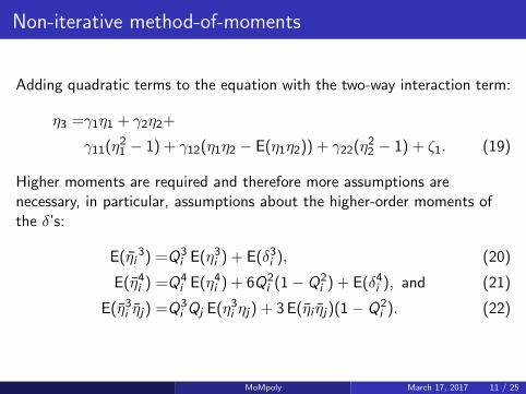
Non-iterative method-of-moments
Adding quadratic terms to the equation with the two-way interaction term:
η3 =γ1η1 + γ2η2+
γ11(η21 − 1) + γ12(η1η2 − E(η1η2)) + γ22(η22 − 1) + ζ1. (19)
Higher moments are required and therefore more assumptions arenecessary, in particular, assumptions about the higher-order moments ofthe δ’s:
E(ηi3) =Q3
i E(η3i ) + E(δ3i ), (20)
E(η4i ) =Q4i E(η4i ) + 6Q2
i (1− Q2i ) + E(δ4i ), and (21)
E(η3i ηj) =Q3i Qj E(η3i ηj) + 3 E(ηi ηj)(1− Q2
i ). (22)
MoMpoly March 17, 2017 11 / 25
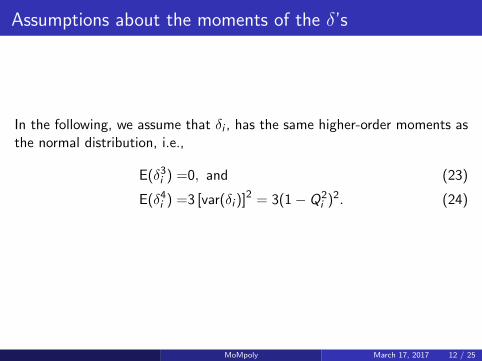
Assumptions about the moments of the δ’s
In the following, we assume that δi , has the same higher-order moments asthe normal distribution, i.e.,
E(δ3i ) =0, and (23)
E(δ4i ) =3 [var(δi )]2 = 3(1− Q2i )2. (24)
MoMpoly March 17, 2017 12 / 25
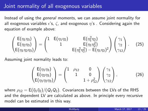
Joint normality of all exogenous variables
Instead of using the general moments, we can assume joint normality forall exogenous variables ε’s, ζ, and exogenous η’s . Considering again theequation of example above: E(η1η3)
E(η2η3)E(η1η2η3)
=
1 E(η1η2) E(η21η2)1 E(η1η
22)
E(η21η22)− E(η1η2)2
γ1γ2γ12
. (25)
Assuming joint normality leads to: E(η1η3)E(η2η3)
E(η1η2η3)
=
1 ρ12 01 0
1 + ρ212
γ1γ2γ12
, (26)
where ρ12 = E(η1η2)/(Q1Q2). Covariances between the LVs of the RHSand the dependent LV are calculated as above. In principle every recursivemodel can be estimated in this way.
MoMpoly March 17, 2017 13 / 25
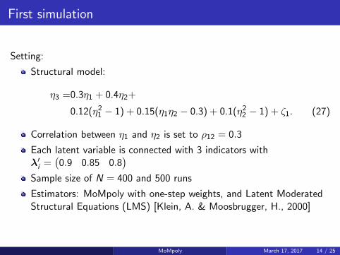
First simulation
Setting:
Structural model:
η3 =0.3η1 + 0.4η2+
0.12(η21 − 1) + 0.15(η1η2 − 0.3) + 0.1(η22 − 1) + ζ1. (27)
Correlation between η1 and η2 is set to ρ12 = 0.3
Each latent variable is connected with 3 indicators withλ′i =
(0.9 0.85 0.8
)Sample size of N = 400 and 500 runs
Estimators: MoMpoly with one-step weights, and Latent ModeratedStructural Equations (LMS) [Klein, A. & Moosbrugger, H., 2000]
MoMpoly March 17, 2017 14 / 25
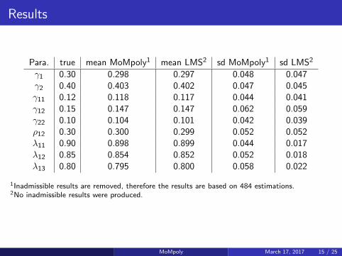
Results
Para. true mean MoMpoly1 mean LMS2 sd MoMpoly1 sd LMS2
γ1 0.30 0.298 0.297 0.048 0.047γ2 0.40 0.403 0.402 0.047 0.045γ11 0.12 0.118 0.117 0.044 0.041γ12 0.15 0.147 0.147 0.062 0.059γ22 0.10 0.104 0.101 0.042 0.039ρ12 0.30 0.300 0.299 0.052 0.052λ11 0.90 0.898 0.899 0.044 0.017λ12 0.85 0.854 0.852 0.052 0.018λ13 0.80 0.795 0.800 0.058 0.022
1Inadmissible results are removed, therefore the results are based on 484 estimations.2No inadmissible results were produced.
MoMpoly March 17, 2017 15 / 25
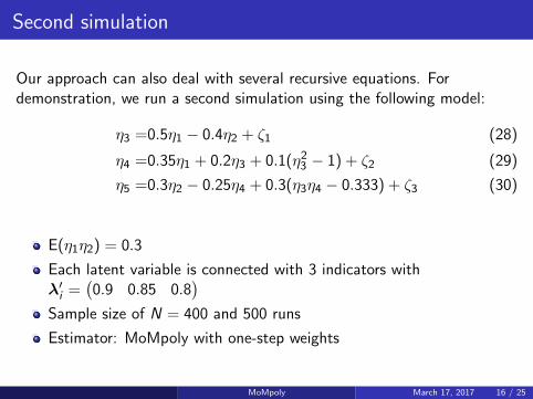
Second simulation
Our approach can also deal with several recursive equations. Fordemonstration, we run a second simulation using the following model:
η3 =0.5η1 − 0.4η2 + ζ1 (28)
η4 =0.35η1 + 0.2η3 + 0.1(η23 − 1) + ζ2 (29)
η5 =0.3η2 − 0.25η4 + 0.3(η3η4 − 0.333) + ζ3 (30)
E(η1η2) = 0.3
Each latent variable is connected with 3 indicators withλ′i =
(0.9 0.85 0.8
)Sample size of N = 400 and 500 runs
Estimator: MoMpoly with one-step weights
MoMpoly March 17, 2017 16 / 25
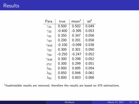
Results
Para. true mean1 sd1
γ31 0.500 0.502 0.049γ32 -0.400 -0.395 0.053γ41 0.350 0.347 0.056γ43 0.200 0.201 0.058γ433 -0.100 -0.099 0.038γ52 0.300 0.301 0.050γ54 -0.250 -0.247 0.052γ534 0.300 0.298 0.052ρ12 0.300 0.299 0.051λ51 0.900 0.895 0.054λ51 0.850 0.846 0.061λ51 0.800 0.803 0.068
1Inadmissible results are removed, therefore the results are based on 475 estimations.
MoMpoly March 17, 2017 17 / 25
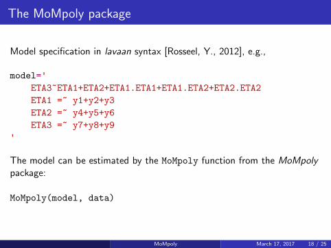
The MoMpoly package
Model specification in lavaan syntax [Rosseel, Y., 2012], e.g.,
model='
ETA3~ETA1+ETA2+ETA1.ETA1+ETA1.ETA2+ETA2.ETA2
ETA1 =~ y1+y2+y3
ETA2 =~ y4+y5+y6
ETA3 =~ y7+y8+y9
'
The model can be estimated by the MoMpoly function from the MoMpolypackage:
MoMpoly(model, data)
MoMpoly March 17, 2017 18 / 25

Capabilities of the MoMpoly package
It is capable to deal with:
single equations usingthe general moments (however, skewness and kurtosis of the δ’s fromthe normal distribution are used)the moments from the multivariate normal distribution (all exogenousvariables: ε’s, ζ, and exogenous η’s are jointly normally distributed)
correlated measurement error within a block
several recursive equations using the moments from the multivariatenormal distribution (all exogenous variables: ε’s, and ζ’s, andexogenous η’s are jointly normally distributed) where the parameterestimates
are retrieved from reduced form coefficient matrixare obtained from replacing equation by equation
several recursive equations using the general moments. Theparameters are estimated equation by equation (limited to LVs up tohigher-order 3)
single-indicator latent variables
MoMpoly March 17, 2017 19 / 25

Further options in the MoMpoly function and functions
MoMpoly(model, data,criterionload=criterion.geometric,
criterionpath=criterion.diff,normality=F,
weightFun=weightFun.onestep,
KindOfEstimation=approach.none,...)
Further options in the MoMpoly function:
different ways to obtain the correction factor ci
different correction factor for loadings and path coefficients
different weights: one-step weights, PLS weights, or prescribedweights
Further functions:
MoMpoly.boot(): combination of the MoMpoly function with theboot package
MoMpoly.jack(): function to obtain Jackknife standard errors
MoMpoly March 17, 2017 20 / 25
Further research
Elaboration of the measurement model via instrumental variabletechniques
Other higher-order moments for delta than those from the normaldistribution)
Robustness against model misspecifications
MoMpoly March 17, 2017 21 / 25

Thank you!Questions/Comments?
MoMpoly March 17, 2017 22 / 25

References
Dijkstra, T. K. & Schermelleh-Engel, K., (2014)
Consistent partial least squares for nonlinear structural equation models
Psychometrika 79(4) 585 – 604.
Dijkstra, T.K. & Henseler, J. (2015)
Consistent and asymptotically normal PLS estimators for linear structural equations
Computational Statistics & Data Analysis, 81, 10 – 23.
Klein, A. & Moosbrugger, H. (2000)
Maximum likelihood estimation of latent interaction effects with the LMS method
Psychometrika, 65(4), 457 – 474.
Rosseel, Y. (2012)
lavaan: An R Package for Structural Equation Modeling
Journal of Statistical Software, 48(2), 1 – 36.
Schuberth, F., Schamberger, T. & Dijkstra, T. K. (2017)
MoMpoly package (version 0.1.3.) available upon request.
MoMpoly March 17, 2017 23 / 25
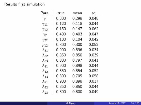
Results first simulation
Para. true mean sd
γ1 0.300 0.298 0.048γ11 0.120 0.118 0.044γ12 0.150 0.147 0.062γ2 0.400 0.403 0.047γ22 0.100 0.104 0.042ρ12 0.300 0.300 0.052λ31 0.900 0.896 0.034λ32 0.850 0.850 0.039λ33 0.800 0.797 0.041λ11 0.900 0.898 0.044λ12 0.850 0.854 0.052λ13 0.800 0.795 0.058λ21 0.900 0.898 0.037λ22 0.850 0.850 0.044λ23 0.800 0.800 0.049
MoMpoly March 17, 2017 24 / 25
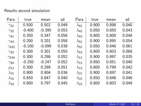
Results second simulation
Para. true mean sd
γ31 0.500 0.502 0.049γ32 -0.400 -0.395 0.053γ41 0.350 0.347 0.056γ43 0.200 0.201 0.058γ433 -0.100 -0.099 0.038γ52 0.300 0.301 0.050γ534 0.300 0.298 0.052γ54 -0.250 -0.247 0.052ρ12 0.300 0.299 0.051λ31 0.900 0.904 0.036λ32 0.850 0.847 0.040λ33 0.800 0.797 0.045
Para true mean sd
λ41 0.900 0.898 0.040λ42 0.850 0.850 0.043λ43 0.800 0.800 0.048λ51 0.900 0.895 0.054λ52 0.850 0.846 0.061λ53 0.800 0.803 0.068λ11 0.900 0.897 0.035λ12 0.850 0.851 0.040λ13 0.800 0.799 0.042λ21 0.900 0.897 0.041λ22 0.850 0.848 0.046λ23 0.800 0.803 0.049
MoMpoly March 17, 2017 25 / 25