Iterative Channel Estimation in LTEUplink

ERIK LINDEN

Master’s Degree ProjectStockholm, Sweden 2014

XR-EE-KT 2014:005

Abstract

An algorithm for iterative channel estimation using soft feedback for LTE uplinkis proposed. The algorithm has low complexity compared to MMSE estimationand does not require knowledge of the channel statistics. A simple polynomialmodel is used for noise suppression across OFDM symbols and a DCT-basedfilter is used for noise suppression across subcarriers.

The algorithm has been tested on several channel models and has been shownto provide a gain of about 0.5 dB with two estimation stages, compared to theno-feedback case. Further, the algorithm has been applied to a MIMO case.

A comparison has been made between the proposed algorithm and turboequalization.

Sammanfattning

En algoritm for iterativ kanalestimering i LTE-upplank foreslas. Algoritmen harlag komplexitet jamfort med MMSE-estimering. En enkel polynomiell modellanvands for att undertrycka brus over OFDM-symboler och ett DCT-baseratfilter anvands for att undertrycka brus over sub-barvagor.

Algoritmen har testats med flera kanalmodeller och visats ge en vinst pa cirka0.5 dB med tva estimeringsitrationer, jamfort med en icke-iterativ mottagare.Algoritmen har ocksa applicerats till en MIMO-situation.

En jamforelse mellan den foreslagna algoritmen och turboutjamning hargjorts.

Contents

1 Background 11.1 LTE - Long-Term Evolution . . . . . . . . . . . . . . . . . . . . . 1

1.1.1 Evolution of LTE . . . . . . . . . . . . . . . . . . . . . . . 11.2 High Data Rate Communications . . . . . . . . . . . . . . . . . . 2

1.2.1 Fundamental Limits . . . . . . . . . . . . . . . . . . . . . 21.2.2 Noise and Interference Limited Scenarios . . . . . . . . . 41.2.3 Higher Data Rates with Limited Bandwidth . . . . . . . . 41.2.4 Wider Bandwidth with Multi-Carrier Techniques . . . . . 5

1.3 OFDM Transmissions . . . . . . . . . . . . . . . . . . . . . . . . 51.3.1 Basic Concept . . . . . . . . . . . . . . . . . . . . . . . . 71.3.2 Demodulation . . . . . . . . . . . . . . . . . . . . . . . . . 81.3.3 Implementation by IFFT/FFT . . . . . . . . . . . . . . . 81.3.4 Cyclic Prefix Insertion . . . . . . . . . . . . . . . . . . . . 101.3.5 Frequency Domain Model . . . . . . . . . . . . . . . . . . 111.3.6 Instantaneous Power of OFDM Transmissions . . . . . . . 12

1.4 Wideband Single-Carrier Transmissions . . . . . . . . . . . . . . 121.4.1 Equalization Against Frequency Selective Channels . . . . 12

1.4.1.1 Linear Time-Domain Equalization . . . . . . . . 131.4.1.2 Frequency-Domain Equalization . . . . . . . . . 141.4.1.3 Decision-Feedback Equalization . . . . . . . . . 14

1.4.2 DFT-spread OFDM . . . . . . . . . . . . . . . . . . . . . 141.4.2.1 Basic Concept . . . . . . . . . . . . . . . . . . . 141.4.2.2 Receiver . . . . . . . . . . . . . . . . . . . . . . 151.4.2.3 Subcarrier Mapping Methods . . . . . . . . . . . 15

1.5 Multiple Antennas . . . . . . . . . . . . . . . . . . . . . . . . . . 161.5.1 Multiple Receiving Antennas . . . . . . . . . . . . . . . . 161.5.2 Spatial Multiplexing . . . . . . . . . . . . . . . . . . . . . 16

1.6 LTE Uplink Physical Resources . . . . . . . . . . . . . . . . . . . 171.6.1 Time-Frequency Structure . . . . . . . . . . . . . . . . . . 171.6.2 Uplink Channels . . . . . . . . . . . . . . . . . . . . . . . 181.6.3 Demodulation-Reference Signals . . . . . . . . . . . . . . 18

1.6.3.1 Reference-Signal Requirements . . . . . . . . . . 191.6.3.2 DM-RS Basic Principles . . . . . . . . . . . . . . 191.6.3.3 Phase-Rotated Reference Sequences . . . . . . . 20

1.7 LTE Uplink Transport Channel Processing . . . . . . . . . . . . 201.7.1 Uplink Transmitter Processing Steps . . . . . . . . . . . . 20

1.7.1.1 CRC Insertion Per Transport Block . . . . . . . 20

i

1.7.1.2 Code Block Segmentation and CRC InsertionPer Code Block . . . . . . . . . . . . . . . . . . 21

1.7.1.3 Channel Coding . . . . . . . . . . . . . . . . . . 211.7.1.4 Rate Matching and Hybrid-ARQ . . . . . . . . . 221.7.1.5 Scrambling . . . . . . . . . . . . . . . . . . . . . 231.7.1.6 Symbol Mapping . . . . . . . . . . . . . . . . . . 231.7.1.7 DFT Spreading . . . . . . . . . . . . . . . . . . 231.7.1.8 Antenna Mapping . . . . . . . . . . . . . . . . . 23

1.7.2 Uplink Receiver Processing Steps . . . . . . . . . . . . . . 231.7.2.1 Antenna Demapping and Grant Extraction . . . 231.7.2.2 Channel Estimation . . . . . . . . . . . . . . . . 241.7.2.3 Antenna Combining and Equalization . . . . . . 251.7.2.4 IDFT Despreading . . . . . . . . . . . . . . . . . 251.7.2.5 Soft Demapping . . . . . . . . . . . . . . . . . . 251.7.2.6 Descrambling . . . . . . . . . . . . . . . . . . . . 251.7.2.7 Rate Dematching and Hybrid-ARQ . . . . . . . 251.7.2.8 Turbo Decoding . . . . . . . . . . . . . . . . . . 25

1.8 Turbo Receivers . . . . . . . . . . . . . . . . . . . . . . . . . . . . 251.8.1 Turbo Codes . . . . . . . . . . . . . . . . . . . . . . . . . 26

1.8.1.1 Encoding . . . . . . . . . . . . . . . . . . . . . . 261.8.1.2 Decoding . . . . . . . . . . . . . . . . . . . . . . 27

1.8.2 Turbo Equalization . . . . . . . . . . . . . . . . . . . . . . 271.8.2.1 Inter-Symbol Interference in DFTS-OFDM Sys-

tems . . . . . . . . . . . . . . . . . . . . . . . . . 271.8.2.2 Turbo Equalization for Interference Cancellation 28

1.8.3 Iterative Channel Estimation . . . . . . . . . . . . . . . . 281.8.3.1 Channel Estimation in OFDM Systems . . . . . 281.8.3.2 Problems With Pilot-Based Channel Estimation 291.8.3.3 Iterative Channel Estimation as a Solution . . . 291.8.3.4 Previous Work . . . . . . . . . . . . . . . . . . . 30

2 Methods 312.1 Iterative Channel Estimator . . . . . . . . . . . . . . . . . . . . . 32

2.1.1 Requirements . . . . . . . . . . . . . . . . . . . . . . . . . 322.1.1.1 Restrictions . . . . . . . . . . . . . . . . . . . . . 32

2.1.2 Conventions . . . . . . . . . . . . . . . . . . . . . . . . . . 332.1.3 Proposed Algorithm . . . . . . . . . . . . . . . . . . . . . 33

2.1.3.1 Symbol Regeneration . . . . . . . . . . . . . . . 352.1.3.2 Symbol Variance/Covariance Estimation . . . . 362.1.3.3 Interference Cancellation (for MIMO) . . . . . . 372.1.3.4 Point-wise Channel Coefficient Estimation . . . 372.1.3.5 Frequency Offset Compensation . . . . . . . . . 402.1.3.6 Model Fitting . . . . . . . . . . . . . . . . . . . 402.1.3.7 Channel Length Estimation . . . . . . . . . . . . 412.1.3.8 Model Selection . . . . . . . . . . . . . . . . . . 422.1.3.9 Channel Filtering . . . . . . . . . . . . . . . . . 432.1.3.10 Channel Regeneration . . . . . . . . . . . . . . . 452.1.3.11 Frequency Offset Uncompensation . . . . . . . . 452.1.3.12 Noise Estimation . . . . . . . . . . . . . . . . . . 45

2.2 Turbo Equalizer . . . . . . . . . . . . . . . . . . . . . . . . . . . 45

ii

2.3 Other Receiver Components . . . . . . . . . . . . . . . . . . . . . 452.4 Channel Models . . . . . . . . . . . . . . . . . . . . . . . . . . . . 462.5 Simulation Setup . . . . . . . . . . . . . . . . . . . . . . . . . . . 47

3 Results 483.1 Main Results . . . . . . . . . . . . . . . . . . . . . . . . . . . . . 49

3.1.1 Gain Per Iteration . . . . . . . . . . . . . . . . . . . . . . 493.1.2 Gain For Different Channels . . . . . . . . . . . . . . . . . 50

3.2 Specific Tests . . . . . . . . . . . . . . . . . . . . . . . . . . . . . 523.2.1 Turbo Equalization . . . . . . . . . . . . . . . . . . . . . . 523.2.2 Model Selection Performance . . . . . . . . . . . . . . . . 533.2.3 MIMO Performance . . . . . . . . . . . . . . . . . . . . . 533.2.4 Gain At Low Throughput . . . . . . . . . . . . . . . . . . 533.2.5 Effect Of Modifications . . . . . . . . . . . . . . . . . . . 55

4 Discussion 574.1 Results . . . . . . . . . . . . . . . . . . . . . . . . . . . . . . . . . 57

4.1.1 Gain For Different Channels . . . . . . . . . . . . . . . . . 574.1.2 Turbo Equalization . . . . . . . . . . . . . . . . . . . . . . 574.1.3 MIMO Performance . . . . . . . . . . . . . . . . . . . . . 584.1.4 Modifications . . . . . . . . . . . . . . . . . . . . . . . . . 58

4.2 Complexity . . . . . . . . . . . . . . . . . . . . . . . . . . . . . . 584.3 Further Work . . . . . . . . . . . . . . . . . . . . . . . . . . . . . 59

4.3.1 Reduce Complexity of Iterations . . . . . . . . . . . . . . 594.3.2 Improved Heuristics . . . . . . . . . . . . . . . . . . . . . 594.3.3 Implementation On Hardware . . . . . . . . . . . . . . . . 59

4.4 Conclusions . . . . . . . . . . . . . . . . . . . . . . . . . . . . . . 59

iii

Chapter 1

Background

This chapter will give an introduction to LTE, with a focus on the physical layeruplink (the physical signals from the mobile terminal to the base station). Thiswill include a brief history of LTE, the fundamentals of data transmissions, theproperties of modulation scheme used in LTE, the advantages of using multipleantennas, the physical resources in LTE and LTE transmitter/receiver process-ing. Finally, the concept of iterative receivers will be introduced.

1.1 LTE - Long-Term Evolution

In the last decades, mobile communication systems have gone from being expen-sive and bulky devices for a select group of people, to being a ubiquitous tech-nology used by a majority of the world’s population [1]. Today, there are moremobile communication devices than fixed phone lines or internet-connected com-puters [2]. The task of developing mobile communication systems has gone frombeing a national or regional concern, to the care of global standard-developingorganizations, today primarily 3GPP (Third Generation Partnership Project)[3].

This section will briefly review the systems proceeding LTE, leading up tothe development and standardization of the Long-Term Evolution.

1.1.1 Evolution of LTE

Mobile communications systems are often divided into generations. It should benoted that this division is somewhat synthetic, but still useful. The first gener-ation of systems, 1G, is the plethora of analog systems of the 1980s. These werefollowed by the fully digital 2G systems, which were developed to increase capac-ity (the number of users that can be serviced) and to provide a more consistentquality of service. The most successful of these 2G systems was GSM (originallyGroupe Special Mobile, later Global System for Mobile communications), whichis still the most common mobile communication system worldwide.

All of the 2G systems were narrowband, in the sense that they were targetedat low data-rate services, mainly voice transmissions. The primary data servicein GSM was text messages (Short Message Service) and the initial system pro-vided a modest data rate of 6.9 kbit/s.

1

Packet-data transmissions were introduced in GSM in the second-half of the1990s, in the form of GPRS (General Packet Radio Services) and later EDGE(Enhanced Data rates for GSM Evolution). Similar modifications were made toother 2G systems as well. These modified systems, often called 2.5G, showedthat there was great potential for packet-data services in mobile communicationsystems.

With 3G, the systems moved to the high-bandwidth radio-interface of UTRA(Universal Terrestrial Radio Access). The development of 3G is today handledby 3GPP, but the associated standards were initially developed by ITU (In-ternational Telecommunication Union). Systems are typically required to meetthe ITU-developed IMT-2000 standard to be called 3G [4]. The most commonlydeployed 3G system today is W-CDMA (Wideband Code-Division Multiple Ac-cess).

LTE is often called 4G, but many claim that it is first with LTE release 10,also known as LTE-Advanced, that the truly evolutionary step to 4G is taken[1]. While the 3G systems support data services, they are primarily telephonesystems, routing voice calls through circuit-switched telephone networks. Theadvent of mobile broadband sparked an interest for a system with high-ratepacket-data transmissions as the primary design target. This was realized withLTE, which uses Internet Protocol (IP) for all its services, including voice callsin the form of Voice-over IP (VoIP).

LTE was first proposed by NTT DoCoMo of Japan in 2004 and the officialstudy by 3GPP began in 2005 [5]. The standard was finalized in December 2008and the first publicly available service was started by TeliaSonera in Oslo andStockholm in December 2009 [6]. The LTE-Advanced standard was finalized by3GPP in March 2011 [7].

In the near future, we can expect to see an even greater proliferation of mo-bile communication devices, possibly with a large societal impact. This makesit imperative to make efficient use our natural resources, both in terms of theradio-spectrum resources used for transmissions and the electrical power con-sumed by mobile devices and base stations.

1.2 High Data Rate Communications

As discussed in the previous section, one of the goals of LTE is to increasedata rates, as compared to previous standards. This section will discuss themore fundamental limits on achievable data rates and the techniques needed toachieve them.

1.2.1 Fundamental Limits

In 1948 Shannon [8] provided the basic mathematical tools needed to computethe maximal rate at which information can be transmitted over a noisy channel.This upper bound is known as the channel capacity. Although complicated inthe general case, for a channel impaired only by additive white Gaussian noise(AWGN) the channel capacity is given by the simple expression [9]

C = B log2

(1 +

S

N

)

2

0.1 1 10Bandwidth utilization γ

−5

0

5

10

15

20M

inim

umE

b/N

0[d

B]

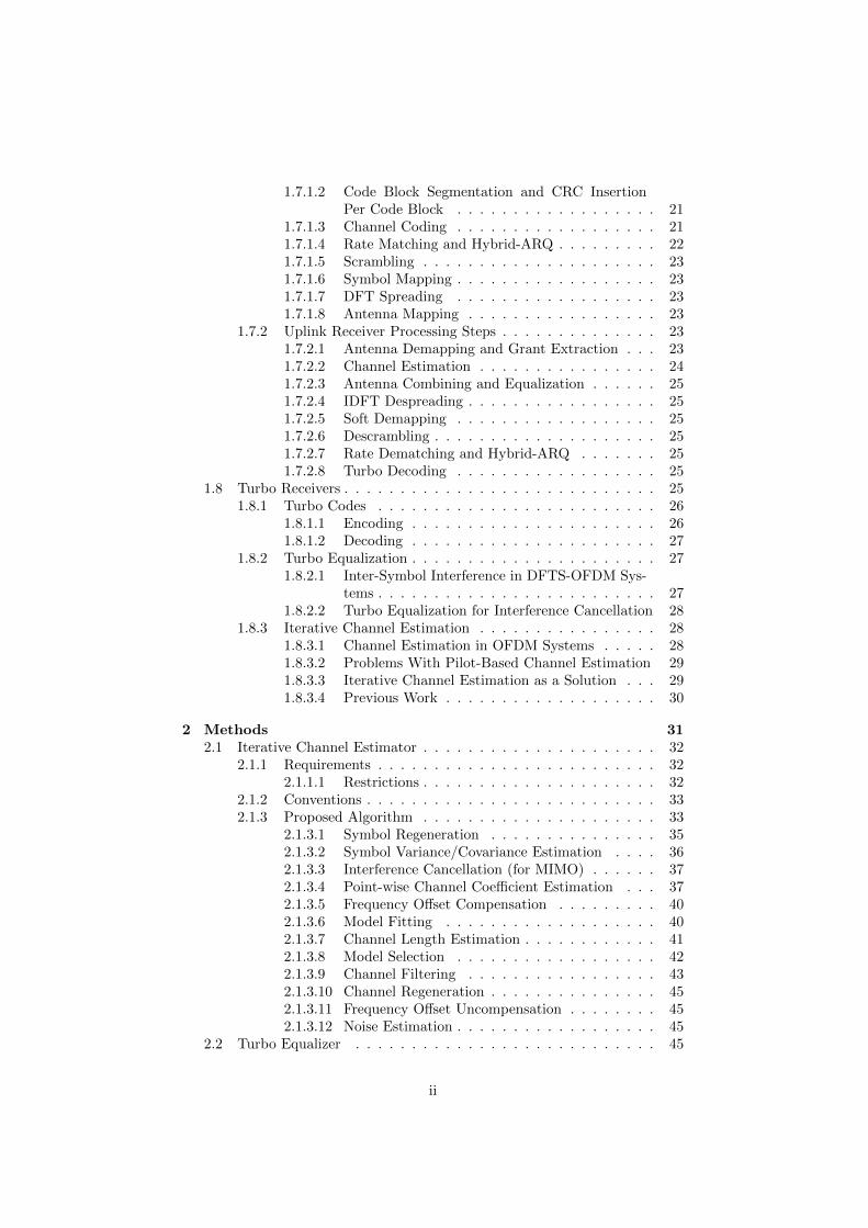
Figure 1.1: The minimum Eb/N0 required as a function of the bandwidth uti-lization γ.

where B is the bandwidth of the channel, S is the received signal power and Nis the noise power.

This equation shows the two fundamental factors limiting the achievabledata rate: the channel bandwidth and the signal-to-noise ratio (SNR). Somemanipulations of the equation can clarify how these two factors interact. Thereceived signal power can be expressed as S = Eb · R, where Eb is the energy-per-data-bit and R is the data rate. The noise power will be proportional to thebandwidth as N = N0 · B, where N0 is the noise power spectral density. Thedata rate must be lower than the channel capacity, leading to the inequality

R ≤ C = B log2

(1 +

Eb ·RN0 ·B

)

Introducing the bandwidth utilization factor γ = R/B (data-rate to channel-bandwidth ratio)

γ ≤ log

(1 + γ

Eb

N0

)

which gives a lower bound on the minimum required Eb/N0 (energy-per-bit tonoise-power-spectral-density ratio) required for a given bandwidth utilization

Eb

N0≥ 2γ − 1

γ

This lower bound is illustrated in Figure 1.1. For bandwidth utilizations belowone, the minimum required Eb/N0 grows slowly with increasing data rate, thatis, increasing γ. On the other hand, for bandwidth utilizations above one, therequired Eb/N0 grows exponentially with increasing data rate.

3

1.2.2 Noise and Interference Limited Scenarios

The discussion above shows that there are two principal operating regions for amobile communication system. If the bandwidth utilization is low, the systemis mainly power limited. In this case, an increase in the available bandwidthwill not substantially increase the achievable data rate. On the other hand,if the bandwidth utilization is high, the system is bandwidth limited. In thiscase, an increase in data rate would require an unproportionally large increasein received signal power.

The conclusion is: to make efficient use of the available power, the channelbandwidth should be at least as great as the desired data rate. The achiev-able data rate can always be increased by moving the transmitter closer to thereceiver, which for a mobile communication implies smaller cell sizes, but fora bandwidth-limited system, the reduction in cell size needed might be pro-hibitively large.

Smaller cell sizes also means that fewer users must share the available band-width (often a scarce resource) and that interference is reduced. Interferencefrom transmitters in neighboring cells is often a larger source of radio-channelimpairment than receiver noise [1].

In addition to smaller cell sizes, data rates can be increased by having mul-tiple transmitting and/or receiving antennas. Section 1.5 will look more atmulti-antenna systems.

1.2.3 Higher Data Rates with Limited Bandwidth

The discussion above shows that for efficient channel utilization, a mobile com-munication system should be able to adapt its data rate to the available band-width and signal-to-noise ratio.

A simple way to adapt the data rate is to have several modulation alpha-bets available. LTE uses quadrature phase-shift keying (QPSK) and quadratureamplitude modulation (QAM) to transmit two, four or six bits of data per mod-ulation symbol1 [10]. Figure 1.2 illustrates how modulation symbols are placedin the complex plane. The symbols in all the alphabets have the same band-width, but the higher order alphabets encode more bits per symbol, increasingthe data rate.

The data rate can be further adapted by the use of channel coding, in theform of forward error correction (FEC) [11, 12]. The basic principle of FECis to add redundant information to the transmission, to allow the receiver tocorrect errors. For example, three coded bits may be transmitted for every twodata bits. This is called a 2/3-rate code. The redundant information decreasesthe effective data rate.

These two methods combine to give mobile communication systems a greatdegree of flexibility in what data rate to use over a given bandwidth. Theprocess of automatically selecting modulation and coding scheme is referred toas link adaptation.

It should be noted that the channel capacity discussed in Section 1.2.1 limitsthe maximal rate at which data can be transmitted over noisy channel, but doesnot provide a computationally realizable method of modulation and coding totransmit at that rate. Great effort has been put into designing modulation and

1How these symbols are used for modulation will be explained in Section 1.3.1.

4

QPSK 16QAM 64QAM

Figure 1.2: Constellation diagrams for the three modulation alphabets used inLTE.

coding schemes that provide good performance while keeping the computationcomplexity of encoding and decoding manageable.

1.2.4 Wider Bandwidth with Multi-Carrier Techniques

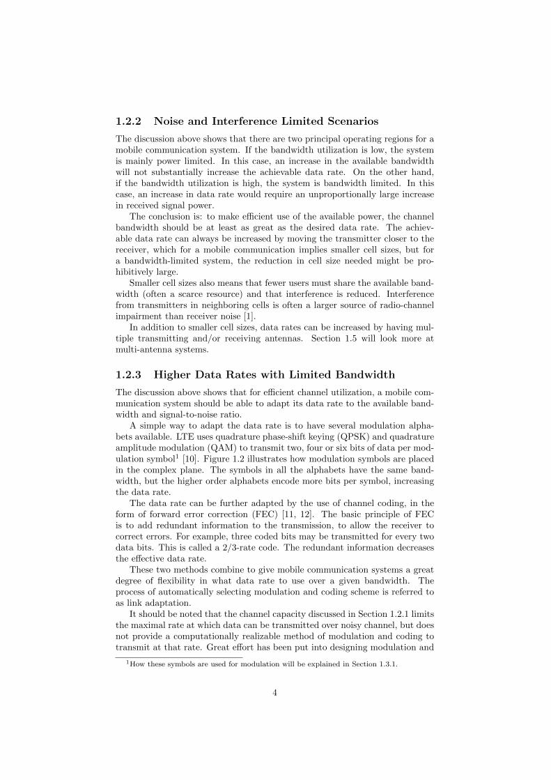
Section 1.2.2 discussed how high-bandwidth transmission are key to high datarates. There are however some technical issues with very wide-band transmis-sions. Radio channels typically introduces time dispersion due to multi-pathpropagation, in which radio signals reach the receiver by multiple paths, as il-lustrated in Figure 1.3. This is known as a time-dispersive channel. At somefrequencies, time-delayed copies of the signal may combine destructively. Thesefrequencies are thus severely attenuated by the channel and the channel is saidto be frequency-selective. Wideband transmissions are more severely affectedby frequency-selective channels than narrowband transmissions.

Frequency-selective channels are usually counteracted by equalization, but athigher bandwidths the complexity of high-quality equalization becomes a seriousissue. A straightforward approach to increasing the signal bandwidth withoutincreasing the receiver complexity is to transmit several narrowband signals inparallel, instead of transmitting a single wideband signal. These narrowbandsignals are often called subcarriers. The equalization effort needed for any givensubcarrier then remains limited [13].

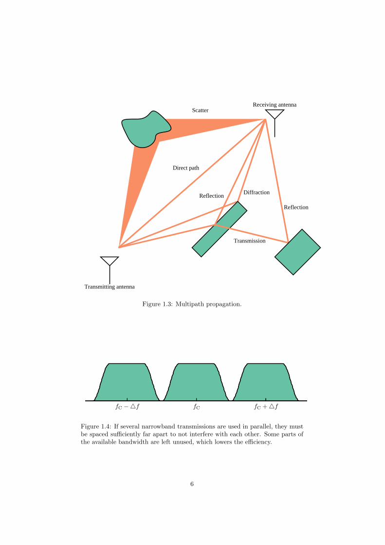
Attempts to use traditional narrowband techniques for multi-carrier trans-missions have been hampered by the need to include guard bands around indi-vidual subcarriers, as illustrated in Figure 1.4, to avoid inter-carrier interference.These guard bands cuts into the bandwidth used for data transmission, reducingefficiency [14].

1.3 OFDM Transmissions

This section will give an introduction to the orthogonal frequency-division mul-tiplexing (OFDM) transmission scheme. OFDM is used for LTE downlink, aswell as in other wireless systems [15] and forms the basis for modulation schemeused in LTE uplink [10].

5

Receiving antenna

Reflection

Reflection

Direct path

Transmission

Scatter

Diffraction

Transmitting antenna

Figure 1.3: Multipath propagation.

fC −4f fC fC +4f

Figure 1.4: If several narrowband transmissions are used in parallel, they mustbe spaced sufficiently far apart to not interfere with each other. Some parts ofthe available bandwidth are left unused, which lowers the efficiency.

6

TU = 1/4fTime-domain

−24f −4f 0 4f 24fFrequency-domain

(sin(πf/4f)πf/4f

)2

Figure 1.5: OFDM uses a rectangular window for pulse-shaping in the timedomain, which results in a sinc-square power spectra.

1.3.1 Basic Concept

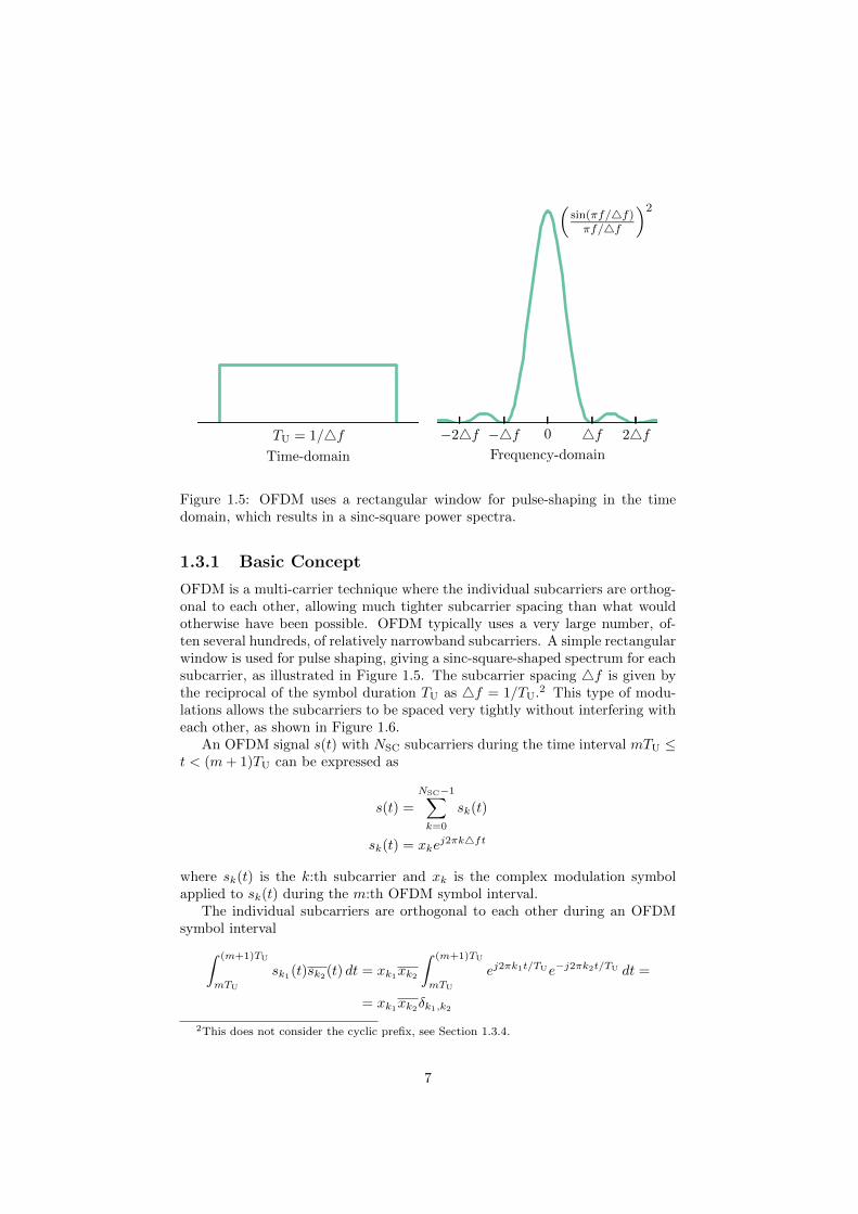
OFDM is a multi-carrier technique where the individual subcarriers are orthog-onal to each other, allowing much tighter subcarrier spacing than what wouldotherwise have been possible. OFDM typically uses a very large number, of-ten several hundreds, of relatively narrowband subcarriers. A simple rectangularwindow is used for pulse shaping, giving a sinc-square-shaped spectrum for eachsubcarrier, as illustrated in Figure 1.5. The subcarrier spacing 4f is given bythe reciprocal of the symbol duration TU as 4f = 1/TU.2 This type of modu-lations allows the subcarriers to be spaced very tightly without interfering witheach other, as shown in Figure 1.6.

An OFDM signal s(t) with NSC subcarriers during the time interval mTU ≤t < (m+ 1)TU can be expressed as

s(t) =

NSC−1∑

k=0

sk(t)

sk(t) = xkej2πk4ft

where sk(t) is the k:th subcarrier and xk is the complex modulation symbolapplied to sk(t) during the m:th OFDM symbol interval.

The individual subcarriers are orthogonal to each other during an OFDMsymbol interval

ˆ (m+1)TU

mTU

sk1(t)sk2(t) dt = xk1xk2

ˆ (m+1)TU

mTU

ej2πk1t/TUe−j2πk2t/TU dt =

= xk1xk2δk1,k2

2This does not consider the cyclic prefix, see Section 1.3.4.

7

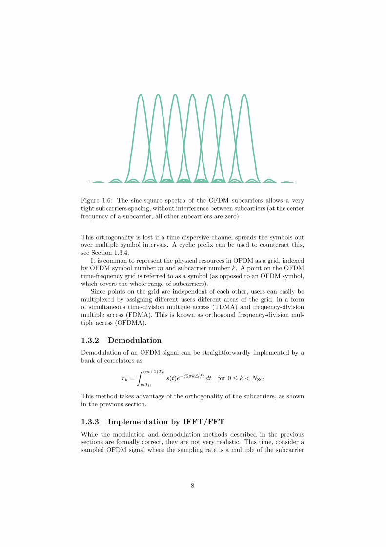
Figure 1.6: The sinc-square spectra of the OFDM subcarriers allows a verytight subcarriers spacing, without interference between subcarriers (at the centerfrequency of a subcarrier, all other subcarriers are zero).

This orthogonality is lost if a time-dispersive channel spreads the symbols outover multiple symbol intervals. A cyclic prefix can be used to counteract this,see Section 1.3.4.

It is common to represent the physical resources in OFDM as a grid, indexedby OFDM symbol number m and subcarrier number k. A point on the OFDMtime-frequency grid is referred to as a symbol (as opposed to an OFDM symbol,which covers the whole range of subcarriers).

Since points on the grid are independent of each other, users can easily bemultiplexed by assigning different users different areas of the grid, in a formof simultaneous time-division multiple access (TDMA) and frequency-divisionmultiple access (FDMA). This is known as orthogonal frequency-division mul-tiple access (OFDMA).

1.3.2 Demodulation

Demodulation of an OFDM signal can be straightforwardly implemented by abank of correlators as

xk =

ˆ (m+1)TU

mTU

s(t)e−j2πk4ft dt for 0 ≤ k < NSC

This method takes advantage of the orthogonality of the subcarriers, as shownin the previous section.

1.3.3 Implementation by IFFT/FFT

While the modulation and demodulation methods described in the previoussections are formally correct, they are not very realistic. This time, consider asampled OFDM signal where the sampling rate is a multiple of the subcarrier

8

S→PSize-NIFFT

P→S

[x0, x1, . . . , xNSC−1]

x0

x1

...

xNSC−1

0

0

s0

s1

...

sN−1

[s0, s1, . . . , sN−1]

Figure 1.7: The IFFT can be used as an OFDM modulator.

S→PSize-NFFT

P→S[s0, s1, . . . , sN−1]

s0

s1

...

sN−1 Discard

x0

x1

...

xNSC−1

[x0, x1, . . . , xNSC−1]

Figure 1.8: The FFT can be used for OFDM demodulation.

spacing fs = 1/Ts = N · 4f . The sampled signal can be expressed as

sn = s(nTs) =

NSC−1∑

k=0

xkej2πk4fnTs =

=

NSC−1∑

k=0

xkej2πkn/N =

=

N−1∑

k=0

xkej2πkn/N

where N ≥ NSC and

xk =

{xk 0 ≤ k < NSC

0 otherwise

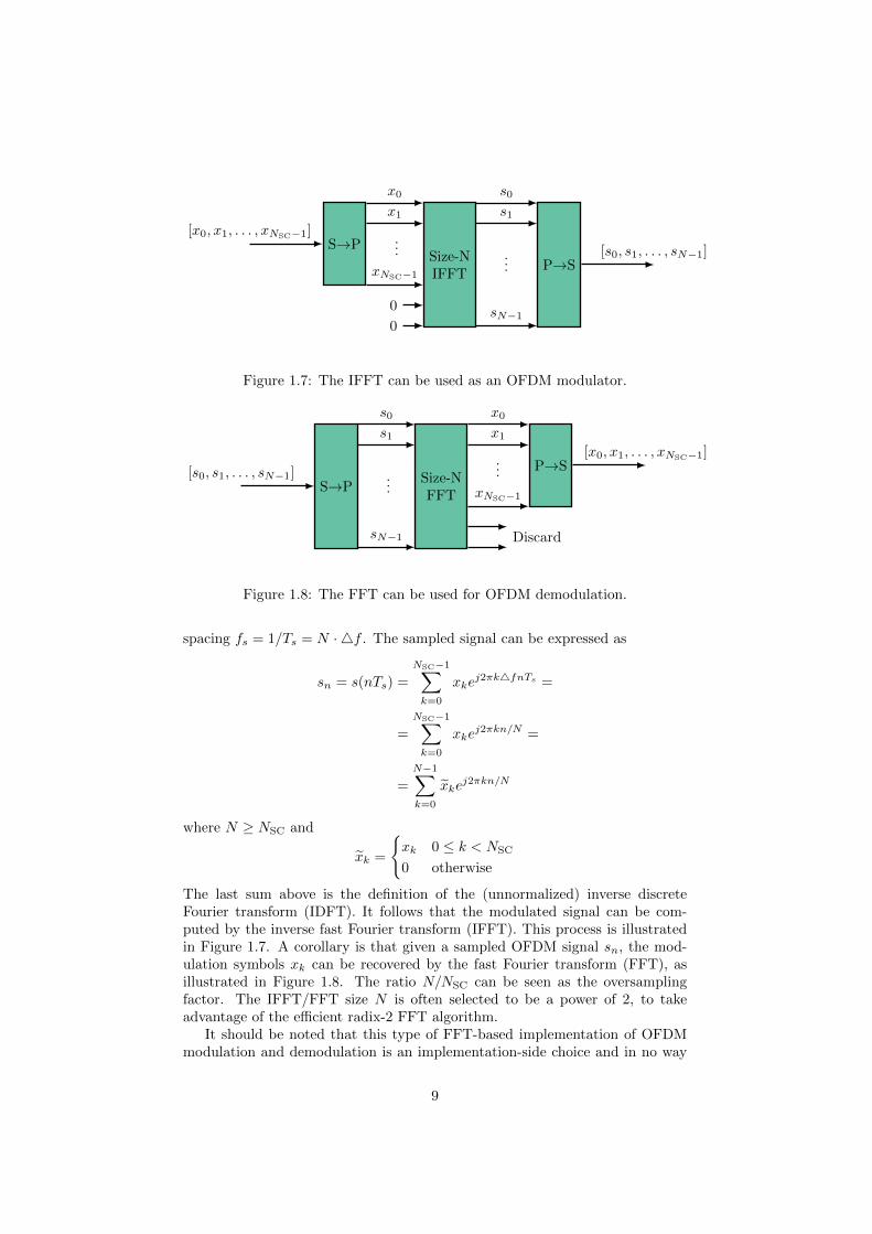
The last sum above is the definition of the (unnormalized) inverse discreteFourier transform (IDFT). It follows that the modulated signal can be com-puted by the inverse fast Fourier transform (IFFT). This process is illustratedin Figure 1.7. A corollary is that given a sampled OFDM signal sn, the mod-ulation symbols xk can be recovered by the fast Fourier transform (FFT), asillustrated in Figure 1.8. The ratio N/NSC can be seen as the oversamplingfactor. The IFFT/FFT size N is often selected to be a power of 2, to takeadvantage of the efficient radix-2 FFT algorithm.

It should be noted that this type of FFT-based implementation of OFDMmodulation and demodulation is an implementation-side choice and in no way

9

Direct path

Delayed path

s(m−1) s(m) s(m+1)

TU

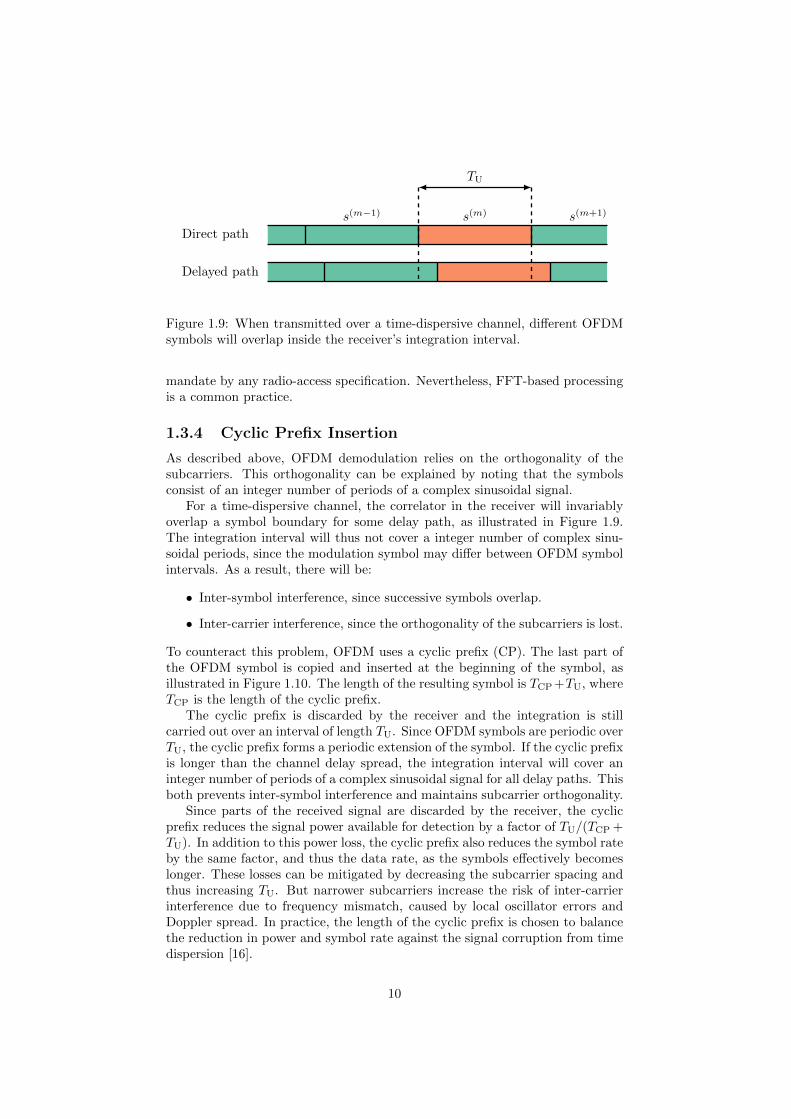
Figure 1.9: When transmitted over a time-dispersive channel, different OFDMsymbols will overlap inside the receiver’s integration interval.

mandate by any radio-access specification. Nevertheless, FFT-based processingis a common practice.

1.3.4 Cyclic Prefix Insertion

As described above, OFDM demodulation relies on the orthogonality of thesubcarriers. This orthogonality can be explained by noting that the symbolsconsist of an integer number of periods of a complex sinusoidal signal.

For a time-dispersive channel, the correlator in the receiver will invariablyoverlap a symbol boundary for some delay path, as illustrated in Figure 1.9.The integration interval will thus not cover a integer number of complex sinu-soidal periods, since the modulation symbol may differ between OFDM symbolintervals. As a result, there will be:

• Inter-symbol interference, since successive symbols overlap.

• Inter-carrier interference, since the orthogonality of the subcarriers is lost.

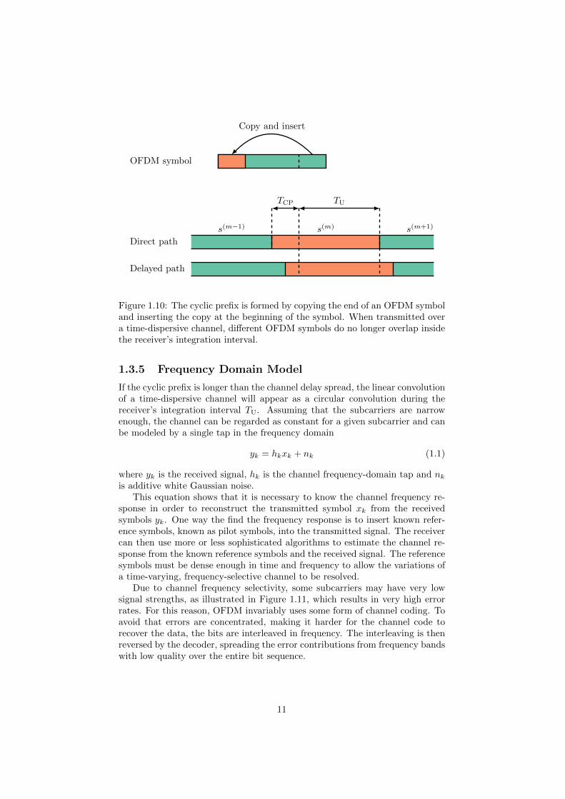
To counteract this problem, OFDM uses a cyclic prefix (CP). The last part ofthe OFDM symbol is copied and inserted at the beginning of the symbol, asillustrated in Figure 1.10. The length of the resulting symbol is TCP +TU, whereTCP is the length of the cyclic prefix.

The cyclic prefix is discarded by the receiver and the integration is stillcarried out over an interval of length TU. Since OFDM symbols are periodic overTU, the cyclic prefix forms a periodic extension of the symbol. If the cyclic prefixis longer than the channel delay spread, the integration interval will cover aninteger number of periods of a complex sinusoidal signal for all delay paths. Thisboth prevents inter-symbol interference and maintains subcarrier orthogonality.

Since parts of the received signal are discarded by the receiver, the cyclicprefix reduces the signal power available for detection by a factor of TU/(TCP +TU). In addition to this power loss, the cyclic prefix also reduces the symbol rateby the same factor, and thus the data rate, as the symbols effectively becomeslonger. These losses can be mitigated by decreasing the subcarrier spacing andthus increasing TU. But narrower subcarriers increase the risk of inter-carrierinterference due to frequency mismatch, caused by local oscillator errors andDoppler spread. In practice, the length of the cyclic prefix is chosen to balancethe reduction in power and symbol rate against the signal corruption from timedispersion [16].

10

Copy and insert

OFDM symbol

Direct path

Delayed path

s(m−1) s(m) s(m+1)

TUTCP

Figure 1.10: The cyclic prefix is formed by copying the end of an OFDM symboland inserting the copy at the beginning of the symbol. When transmitted overa time-dispersive channel, different OFDM symbols do no longer overlap insidethe receiver’s integration interval.

1.3.5 Frequency Domain Model

If the cyclic prefix is longer than the channel delay spread, the linear convolutionof a time-dispersive channel will appear as a circular convolution during thereceiver’s integration interval TU. Assuming that the subcarriers are narrowenough, the channel can be regarded as constant for a given subcarrier and canbe modeled by a single tap in the frequency domain

yk = hkxk + nk (1.1)

where yk is the received signal, hk is the channel frequency-domain tap and nkis additive white Gaussian noise.

This equation shows that it is necessary to know the channel frequency re-sponse in order to reconstruct the transmitted symbol xk from the receivedsymbols yk. One way the find the frequency response is to insert known refer-ence symbols, known as pilot symbols, into the transmitted signal. The receivercan then use more or less sophisticated algorithms to estimate the channel re-sponse from the known reference symbols and the received signal. The referencesymbols must be dense enough in time and frequency to allow the variations ofa time-varying, frequency-selective channel to be resolved.

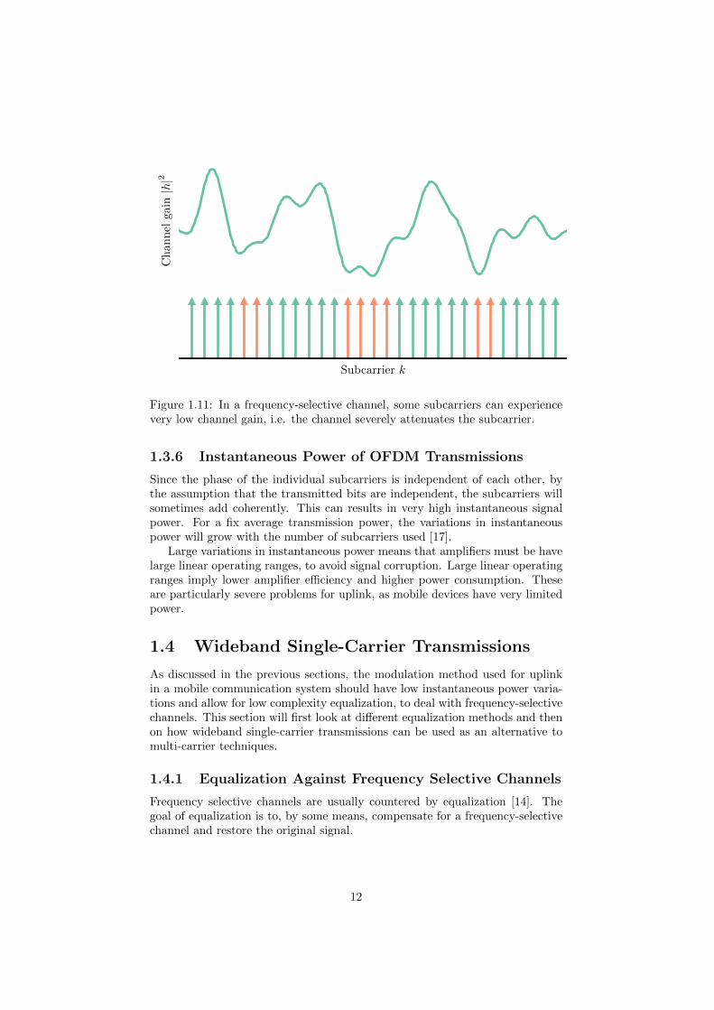
Due to channel frequency selectivity, some subcarriers may have very lowsignal strengths, as illustrated in Figure 1.11, which results in very high errorrates. For this reason, OFDM invariably uses some form of channel coding. Toavoid that errors are concentrated, making it harder for the channel code torecover the data, the bits are interleaved in frequency. The interleaving is thenreversed by the decoder, spreading the error contributions from frequency bandswith low quality over the entire bit sequence.

11

Ch

ann

elga

in|h|2

Subcarrier k

Figure 1.11: In a frequency-selective channel, some subcarriers can experiencevery low channel gain, i.e. the channel severely attenuates the subcarrier.

1.3.6 Instantaneous Power of OFDM Transmissions

Since the phase of the individual subcarriers is independent of each other, bythe assumption that the transmitted bits are independent, the subcarriers willsometimes add coherently. This can results in very high instantaneous signalpower. For a fix average transmission power, the variations in instantaneouspower will grow with the number of subcarriers used [17].

Large variations in instantaneous power means that amplifiers must be havelarge linear operating ranges, to avoid signal corruption. Large linear operatingranges imply lower amplifier efficiency and higher power consumption. Theseare particularly severe problems for uplink, as mobile devices have very limitedpower.

1.4 Wideband Single-Carrier Transmissions

As discussed in the previous sections, the modulation method used for uplinkin a mobile communication system should have low instantaneous power varia-tions and allow for low complexity equalization, to deal with frequency-selectivechannels. This section will first look at different equalization methods and thenon how wideband single-carrier transmissions can be used as an alternative tomulti-carrier techniques.

1.4.1 Equalization Against Frequency Selective Channels

Frequency selective channels are usually countered by equalization [14]. Thegoal of equalization is to, by some means, compensate for a frequency-selectivechannel and restore the original signal.

12

1.4.1.1 Linear Time-Domain Equalization

The most simple approach to equalization is to apply some linear filter w(τ) tothe received signal r(t), to reconstruct the transmitted signal

s(t) = (r ∗ w)(t)

where ∗ denotes linear convolution. A popular receiver structure for widebandsignals is the rake receiver [14]. Here the filter is chosen as the time-reversedconjugate channel impulse response

w(τ) = g(−τ)

where g is the channel impulse response. This forms a channel-matched filter,which maximizes the signal-to-noise ratio at the output of the equalizer for anAWGN channel [18]. However, the filter does not provide any compensationfor a frequency-selective channel and might severely distort the shape of thereceived signal.

An alternative approach is to select the receiver filter as to completely com-pensate for the frequency-selective channel

g ∗ w = 1

This is known as zero-forcing (ZF) equalization. However, this method does notconsider the receiver noise. At frequencies with low path gain, the ZF equalizerwill boost the received signal greatly, amplifying any noise equally much. Thiscan potentially give a very large increase in noise levels.

A tradeoff between the two methods is the minimum mean-square error(MMSE) equalizer. Here the filter is chosen as to minimize the mean-squareerror of the equalized signal, that is, to minimize

E{|s(t)− s(t)|2

}

This method usually provides a good tradeoff between equalization and noisesuppression.

The receiver filter is typically implemented as a discrete finite impulse re-sponse (FIR) filter with L filter taps. The complexity of the filtering operationincreases with the bandwidth of the received signal due to two factors:

• A wideband channel is subjected to more frequency selectivity than anarrowband channel, necessitating more filter taps L to compensate forthe selectivity.

• A wideband transmission must be sampled at a higher rate than a narrow-band transmission, and thus the filtering must be carried out at a higherrate.

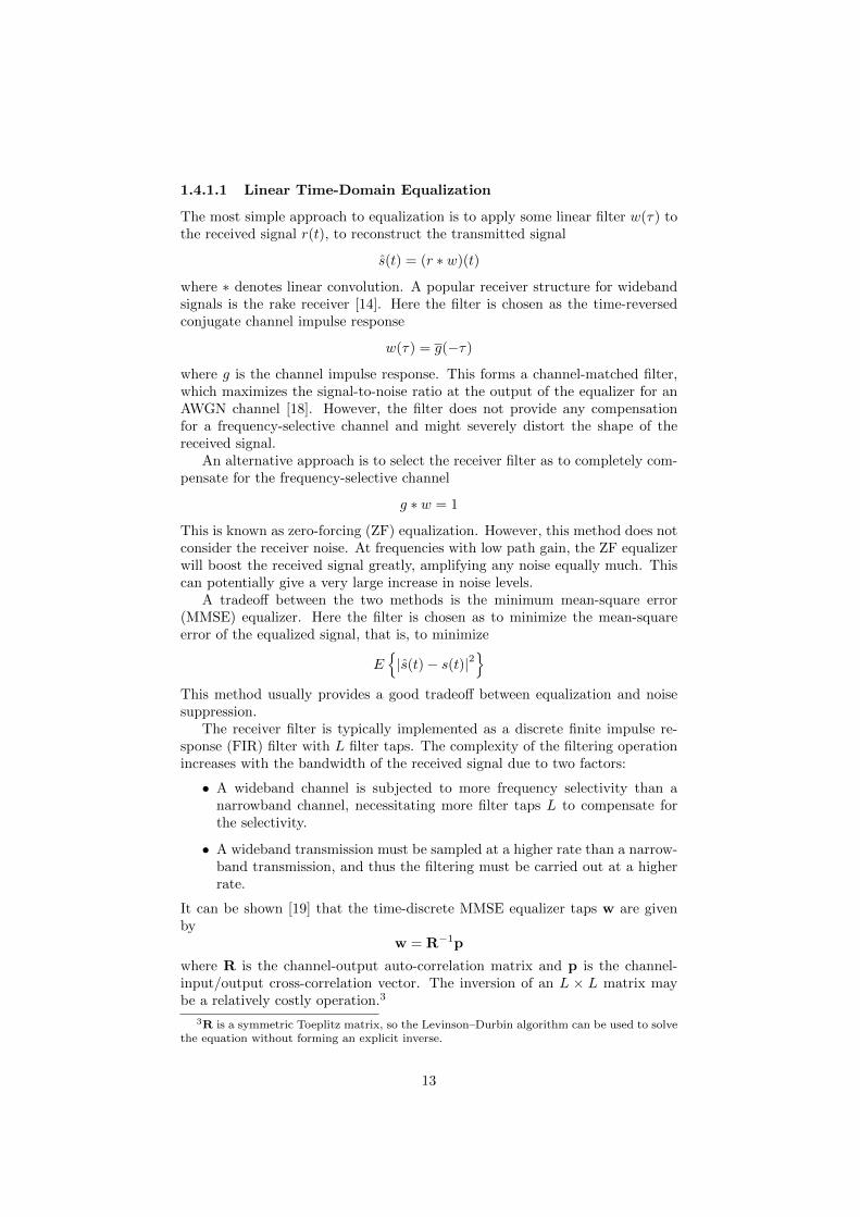
It can be shown [19] that the time-discrete MMSE equalizer taps w are givenby

w = R−1p

where R is the channel-output auto-correlation matrix and p is the channel-input/output cross-correlation vector. The inversion of an L × L matrix maybe a relatively costly operation.3

3R is a symmetric Toeplitz matrix, so the Levinson–Durbin algorithm can be used to solvethe equation without forming an explicit inverse.

13

1.4.1.2 Frequency-Domain Equalization

The complexity of linear equalization can be reduced if the equalization is per-formed in frequency domain [20]. The circular convolution theorem shows thatcircular convolutions can be computed efficiently through the FFT. Linear con-volutions can be implemented by the overlap-add or the overlap-save method,where several circular convolutions are added together to form a linear convo-lution [21].

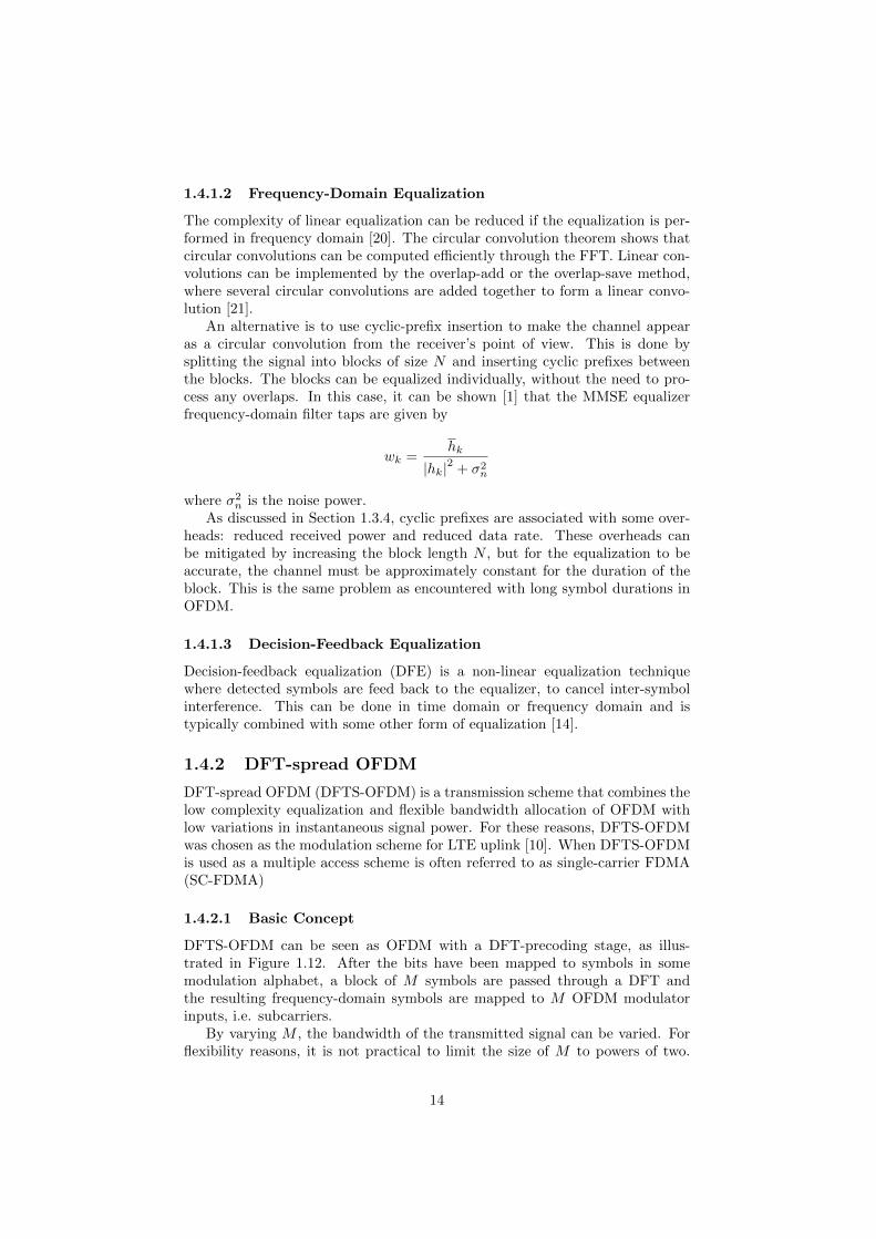
An alternative is to use cyclic-prefix insertion to make the channel appearas a circular convolution from the receiver’s point of view. This is done bysplitting the signal into blocks of size N and inserting cyclic prefixes betweenthe blocks. The blocks can be equalized individually, without the need to pro-cess any overlaps. In this case, it can be shown [1] that the MMSE equalizerfrequency-domain filter taps are given by

wk =hk

|hk|2 + σ2n

where σ2n is the noise power.

As discussed in Section 1.3.4, cyclic prefixes are associated with some over-heads: reduced received power and reduced data rate. These overheads canbe mitigated by increasing the block length N , but for the equalization to beaccurate, the channel must be approximately constant for the duration of theblock. This is the same problem as encountered with long symbol durations inOFDM.

1.4.1.3 Decision-Feedback Equalization

Decision-feedback equalization (DFE) is a non-linear equalization techniquewhere detected symbols are feed back to the equalizer, to cancel inter-symbolinterference. This can be done in time domain or frequency domain and istypically combined with some other form of equalization [14].

1.4.2 DFT-spread OFDM

DFT-spread OFDM (DFTS-OFDM) is a transmission scheme that combines thelow complexity equalization and flexible bandwidth allocation of OFDM withlow variations in instantaneous signal power. For these reasons, DFTS-OFDMwas chosen as the modulation scheme for LTE uplink [10]. When DFTS-OFDMis used as a multiple access scheme is often referred to as single-carrier FDMA(SC-FDMA)

1.4.2.1 Basic Concept

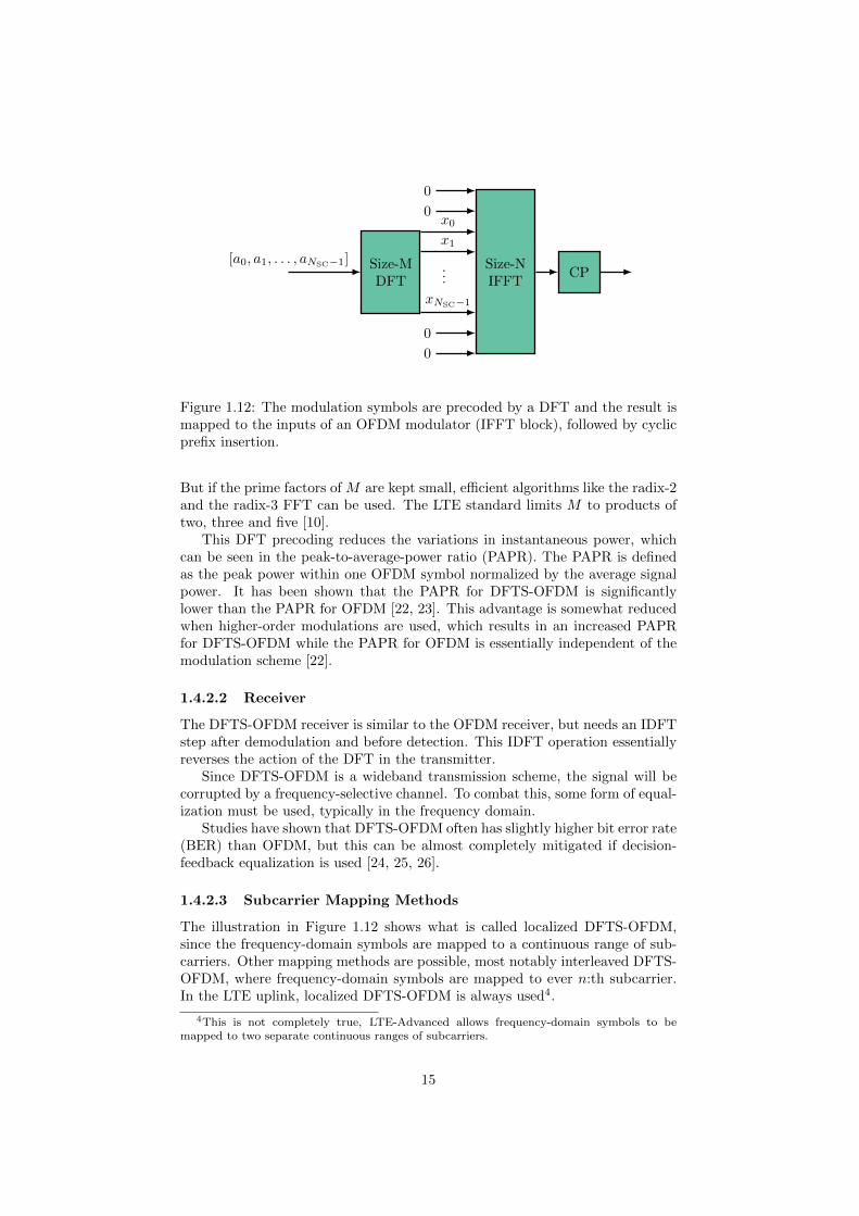
DFTS-OFDM can be seen as OFDM with a DFT-precoding stage, as illus-trated in Figure 1.12. After the bits have been mapped to symbols in somemodulation alphabet, a block of M symbols are passed through a DFT andthe resulting frequency-domain symbols are mapped to M OFDM modulatorinputs, i.e. subcarriers.

By varying M , the bandwidth of the transmitted signal can be varied. Forflexibility reasons, it is not practical to limit the size of M to powers of two.

14

Size-MDFT

Size-NIFFT

CP[a0, a1, . . . , aNSC−1]

x0

x1

...

xNSC−1

0

0

0

0

Figure 1.12: The modulation symbols are precoded by a DFT and the result ismapped to the inputs of an OFDM modulator (IFFT block), followed by cyclicprefix insertion.

But if the prime factors of M are kept small, efficient algorithms like the radix-2and the radix-3 FFT can be used. The LTE standard limits M to products oftwo, three and five [10].

This DFT precoding reduces the variations in instantaneous power, whichcan be seen in the peak-to-average-power ratio (PAPR). The PAPR is definedas the peak power within one OFDM symbol normalized by the average signalpower. It has been shown that the PAPR for DFTS-OFDM is significantlylower than the PAPR for OFDM [22, 23]. This advantage is somewhat reducedwhen higher-order modulations are used, which results in an increased PAPRfor DFTS-OFDM while the PAPR for OFDM is essentially independent of themodulation scheme [22].

1.4.2.2 Receiver

The DFTS-OFDM receiver is similar to the OFDM receiver, but needs an IDFTstep after demodulation and before detection. This IDFT operation essentiallyreverses the action of the DFT in the transmitter.

Since DFTS-OFDM is a wideband transmission scheme, the signal will becorrupted by a frequency-selective channel. To combat this, some form of equal-ization must be used, typically in the frequency domain.

Studies have shown that DFTS-OFDM often has slightly higher bit error rate(BER) than OFDM, but this can be almost completely mitigated if decision-feedback equalization is used [24, 25, 26].

1.4.2.3 Subcarrier Mapping Methods

The illustration in Figure 1.12 shows what is called localized DFTS-OFDM,since the frequency-domain symbols are mapped to a continuous range of sub-carriers. Other mapping methods are possible, most notably interleaved DFTS-OFDM, where frequency-domain symbols are mapped to ever n:th subcarrier.In the LTE uplink, localized DFTS-OFDM is always used4.

4This is not completely true, LTE-Advanced allows frequency-domain symbols to bemapped to two separate continuous ranges of subcarriers.

15

1.5 Multiple Antennas

This section will introduce multi-antenna techniques, first multiple receivingantennas and then spatial multiplexing.

1.5.1 Multiple Receiving Antennas

Base stations have been using multiple receiving antennas for many years. Themost obvious benefit of multiple antennas is increased sensitivity, but there areothers. If the antennas are spaced sufficiently far apart (exactly how far dependson the wavelength and propagation conditions), they will experience differentchannel conditions. If one antenna has a poor channel at a certain frequency,another antenna may have a good channel. This provides robustness againstfading channels. Further, if there are sources of interference that are commonto several of the antennas, the impact of the interference can be reduced.

Receivers will typically combine the input from multiple antennas to a singlesignal. Two common methods are

Maximum ratio combining (MRC) With MRC, different antennas are com-bined to maximize the signal-to-noise ratio of the combined signal.

Interference rejection combining (IRC) IRC is similar to MRC, but alsoconsiders the possibility of correlated interference between antennas, max-imizing the signal-to-interference-plus-noise ratio (SINR). Theoretically,IRC always outperforms MRC, since it more accurately models the chan-nel impairments. But in practice, the interference correlation must beestimated from noisy data. In situations with low correlated interference,noise in the correlation estimate can make IRC perform worse than MRC.

A configuration employing a single transmitting antenna and multiple receivingantennas is often referred to as SIMO, for single-input, multiple-output systems.

1.5.2 Spatial Multiplexing

The use of multiple receiving antennas is a way to increase the signal-to-interference-plus-noise ratio and to achieve diversity against fading. However, if multipleantennas are used both for transmission and reception, it is possible to substan-tially increase the overall data rates, especially in high SINR conditions.

With NT transmitting antennas and NR receiving antennas, the SINR canbe made to increase proportionally to the product NT×NR, assuming constantpower per antenna [1]. But as discussed in Section 1.2.1, if the system is band-width limited, increases in SINR gives very small increases in the achievabledata rate.

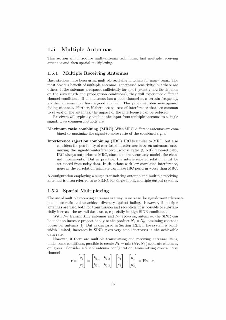
However, if there are multiple transmitting and receiving antennas, it is,under some conditions, possible to create NL = min (NT, NR) separate channels,or layers. Consider a 2 × 2 antenna configuration, transmitting over a noisychannel

r =

r1

r2

=

h1,1 h1,2

h2,1 h2,2

·

s1

s2

+

n1

n2

= Hs + n

16

The receiver can recover both transmitted signals by using the inverse of thechannel matrix W = H−1

s1

s2

= Wr =

s1

s2

+ H−1n

It is clear that properties of H determines how effective the spatial multiplexingis. Specifically, the closer H is to being singular, the larger the noise amplifica-tion will be.

A configuration employing multiple transmitting and receiving antennas isoften referred to as MIMO, for multiple-input, multiple-output system.

For the purposes of this thesis, MIMO will mean that different users (orusers with multiple transmitters) share the air-interface resources of the mobilecommunication system. Inverting the channel matrix is not a good method forequalization, as it has the same problems as ZF equalization. The receiverswill instead often employ a non-linear processing scheme where the data streamfrom one user is decoded first, and then subtracted from the received signal, ina process that is repeated until all users have been decoded. This method isknown as successive interference cancellation (SIC).

1.6 LTE Uplink Physical Resources

This section will provide an overview of the time and frequency-domain resourcesuse in LTE uplink.

1.6.1 Time-Frequency Structure

OFDM is the basic modulation scheme used in the LTE uplink, in the formof DFT-spread OFDM. The OFDM subcarrier spacing is 15 kHz. In the timedomain, LTE transmissions are organized into (radio) frames of length 10 ms[10]. Each frame is divided into ten equally sized subframes of 1 ms. Each sub-frame is divided into two equally sized slots of 0.5 ms which contains a numberof OFDM symbols, including cyclic prefixes.

The 15 kHz LTE subcarriers spacing corresponds to a useful symbol timeTU of approximately 66.7 µs. The total length of an OFDM symbol is then thesum of the useful symbol time and the cyclic prefix. LTE defines two cyclicprefix lengths, a normal prefix of length 4.7 µs and an extended prefix of length16.7 µs. Depending on the cyclic prefix used, seven or six OFDM symbols aretransmitted during one slot.

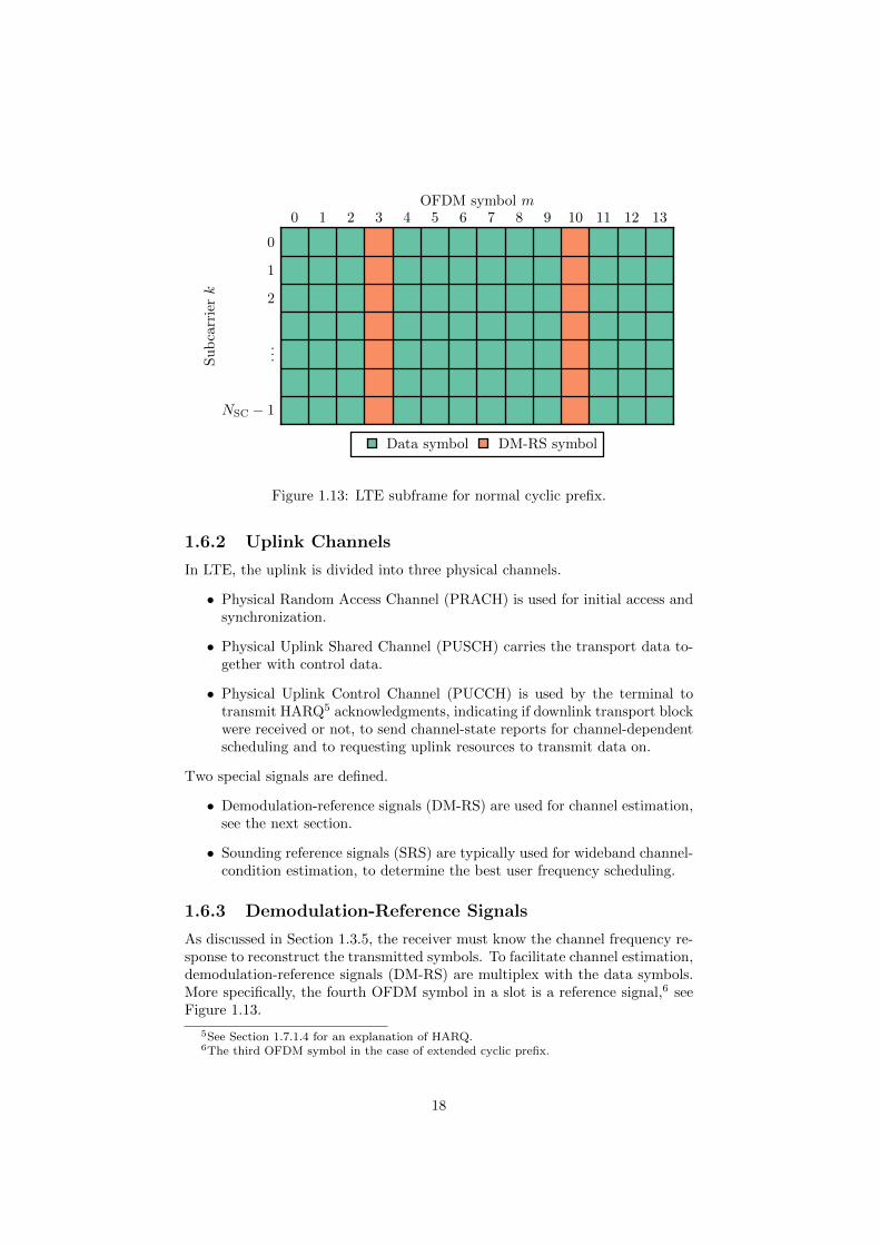
A resource element consists of one subcarrier during one OFDM symbol andis the smallest physical resource in LTE. Resource elements are grouped intoresource blocks (RB). Each resource block consists of 12 consecutive subcarriersin the frequency-domain and one slot in the time-domain. Although resourceblocks are defined over one slot, the smallest time unit for scheduling in LTE is asubframe, which consists of two consecutive slots. The LTE specification allowsthe overall number of resource blocks in the frequency domain used by a carrierto range from a minimum of 6 up to a maximum of 100. This approximatelycorresponds to a minimum transmission bandwidth of 1.4 MHz and a maximumof 20 MHz.

17

0 1 2 3 4 5 6 7 8 9 10 11 12 13OFDM symbol m

NSC − 1

...

2

1

0

Su

bca

rrie

rk

Data symbol DM-RS symbol

Figure 1.13: LTE subframe for normal cyclic prefix.

1.6.2 Uplink Channels

In LTE, the uplink is divided into three physical channels.

• Physical Random Access Channel (PRACH) is used for initial access andsynchronization.

• Physical Uplink Shared Channel (PUSCH) carries the transport data to-gether with control data.

• Physical Uplink Control Channel (PUCCH) is used by the terminal totransmit HARQ5 acknowledgments, indicating if downlink transport blockwere received or not, to send channel-state reports for channel-dependentscheduling and to requesting uplink resources to transmit data on.

Two special signals are defined.

• Demodulation-reference signals (DM-RS) are used for channel estimation,see the next section.

• Sounding reference signals (SRS) are typically used for wideband channel-condition estimation, to determine the best user frequency scheduling.

1.6.3 Demodulation-Reference Signals

As discussed in Section 1.3.5, the receiver must know the channel frequency re-sponse to reconstruct the transmitted symbols. To facilitate channel estimation,demodulation-reference signals (DM-RS) are multiplex with the data symbols.More specifically, the fourth OFDM symbol in a slot is a reference signal,6 seeFigure 1.13.

5See Section 1.7.1.4 for an explanation of HARQ.6The third OFDM symbol in the case of extended cyclic prefix.

18

1.6.3.1 Reference-Signal Requirements

A reference signal can be defined as a frequency-domain reference-signal se-quence applied to consecutive subcarriers. The bandwidth of the referencesignal must equal the bandwidth of the corresponding PUSCH transmission,measured in the number of subcarriers. Since PUSCH transmissions are alwaysallocated in blocks of 12 subcarriers, the length of the reference-signal sequencewill always be a multiple of 12.

Reference signals should preferably have the following properties:

• Limited power variations in the time domain. Reference signals are trans-mitted without DFT-spreading, so it is important to keep the PAPR low.

• Limited power variations in the frequency domain, to allow for similarchannel-estimation quality at all frequencies. This is equivalent to goodtime-domain auto-correlation properties.

• Different cells should use different reference signals, to avoid inter-cellinterference. To keep the network planing efforts reasonable, there shouldbe enough sequences of a given length available.

1.6.3.2 DM-RS Basic Principles

So called Zadoff-Chu sequences [27] have constant power in time and frequencydomain. The elements of a sequence of length NZC are given by

xZCk = e

−iπq k(k+1)NZC 0 ≤ k < NZC − 1

where

1 < q < NZC

gcd(NZC, q) = 1

Zadoff-Chu sequences have zero cyclic auto-correlation for all non-zero lags.Further, the cross-correlation between two prime length Zadoff-Chu sequencesis constant 1/NZC, provided that q1 − q2 is relative prime to NZC [28].

There are some problems with using Zadoff-Chu sequences directly as de-modulation reference signals. The number of sequences available of a givenlength is equal to the number of integers that are relative prime to the se-quence length. So to maximize the number of sequences, a prime sequencelength should be used. But all sequence lengths must be a multiple of 12, sothe sequence length will never be prime. Further, for short sequence lengths,the number of available sequences would not be enough even for prime lengthsequences.

LTE solves this by using cyclic extensions of prime-length Zadoff-Chu se-quences. For short sequences lengths, corresponding to one or two resourceblocks, a set of QPSK-based sequences are explicitly listed in the LTE speci-fications [10]. Otherwise, for a reference-sequence length NRS, the Zadoff-Chusequence length NZC is chosen as the largest prime such that NZC < NRS. Theextended Zadoff-Chu sequence xZC

k is then

xZCk = xZC

k mod NZC0 ≤ k < NRS − 1

The extended sequence does not have zero cyclic auto-correlation, but the auto-correlation is typically small.

19

1.6.3.3 Phase-Rotated Reference Sequences

While different Zadoff-Chu sequences have low cross-correlation, it is possible togenerate completely orthogonal sequences by cyclically shifting the same Zadoff-Chu sequence. A cyclic shift in time domain corresponds to a phase rotation infrequency domain, giving the transmitted reference signal

xRSk = xZC

k eiπαk 0 ≤ k < NRS − 1

where α = m/6 for values of m between 0 and 11. Thus, there are at most12 orthogonal reference signals. The possibility of orthogonal reference signalsis important in the case of spatial multiplexing, where multiple transmitters inthe same cell will be using the same time-frequency resources [29].

The cyclic shifting property can be shown by considering a reference sequencesent through a channel with frequency response h and then matched filter witha phase-rotated replica of itself. The output is the channel frequency responsemodulated by a complex exponential

(hkx

RSk

)·(xRSk e−iπαk

)= hke

−iπαk

Multiplication by a complex exponential in frequency domain corresponds to acyclic shift in time domain

F−1(hke−iπαk) = gn−a/2 mod NRS

where F−1 (·) is the IDFT and g is the channel impulse response. Thus, byphase rotating the reference sequences, other users’ channels will be pushed tohigher cyclic delays, so that different channels can be separated in time domain.This is illustrated in Figure 1.14.

1.7 LTE Uplink Transport Channel Processing

This section will review the different steps of the physical uplink shared channelprocessing. PUSCH transports both user and control data, but this section willfocus on the user data.

1.7.1 Uplink Transmitter Processing Steps

Figure 1.15 illustrates the different steps of the PUSCH processing. Withineach Transmission Time Interval (TTI), corresponding to one 1 ms, one or twotransport blocks are delivered from the Media Access Control layer (MAC). Thenumber of transport blocks depends on the multi-antenna configuration used.In the case of no spatial multiplexing, one transport block is transmitted perTTI. If spatial multiplexing is used, two transport blocks are transmitted perTTI.

1.7.1.1 CRC Insertion Per Transport Block

The first processing step is to compute and append a 24-bit CRC (cyclic redun-dancy check) checksum to each transport block [30]. The CRC checksum allowsreceiver-side detection of errors in the decoded transport block. If errors aredetected, the receiver can trigger a retransmission request.

20

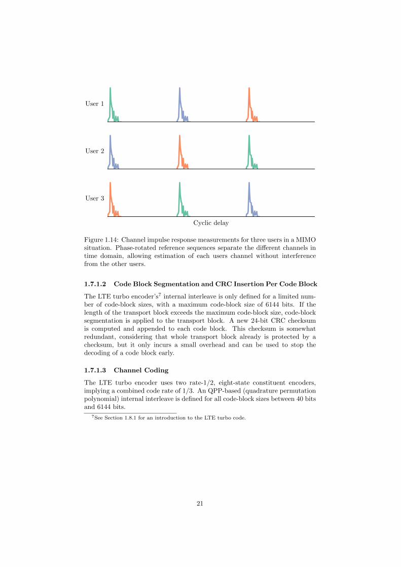
User 1

User 2

Cyclic delay

User 3

Figure 1.14: Channel impulse response measurements for three users in a MIMOsituation. Phase-rotated reference sequences separate the different channels intime domain, allowing estimation of each users channel without interferencefrom the other users.

1.7.1.2 Code Block Segmentation and CRC Insertion Per Code Block

The LTE turbo encoder’s7 internal interleave is only defined for a limited num-ber of code-block sizes, with a maximum code-block size of 6144 bits. If thelength of the transport block exceeds the maximum code-block size, code-blocksegmentation is applied to the transport block. A new 24-bit CRC checksumis computed and appended to each code block. This checksum is somewhatredundant, considering that whole transport block already is protected by achecksum, but it only incurs a small overhead and can be used to stop thedecoding of a code block early.

1.7.1.3 Channel Coding

The LTE turbo encoder uses two rate-1/2, eight-state constituent encoders,implying a combined code rate of 1/3. An QPP-based (quadrature permutationpolynomial) internal interleave is defined for all code-block sizes between 40 bitsand 6144 bits.

7See Section 1.8.1 for an introduction to the LTE turbo code.

21

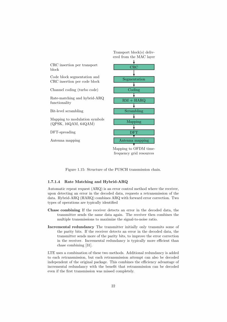
Transport block(s) deliv-ered from the MAC layer

CRC insertion per transportblock

CRC

Code block segmentation andCRC insertion per code block

Segmentation

Channel coding (turbo code) Coding

Rate-matching and hybrid-ARQfunctionality

RM + HARQ

Bit-level scrambling Scrambling

Mapping to modulation symbols(QPSK, 16QAM, 64QAM)

Mapping

DFT-spreading DFT

Antenna mapping Antenna mapping

Mapping to OFDM time-frequency grid resources

Figure 1.15: Structure of the PUSCH transmission chain.

1.7.1.4 Rate Matching and Hybrid-ARQ

Automatic repeat request (ARQ) is an error control method where the receiver,upon detecting an error in the decoded data, requests a retransmission of thedata. Hybrid-ARQ (HARQ) combines ARQ with forward error correction. Twotypes of operations are typically identified

Chase combining If the receiver detects an error in the decoded data, thetransmitter sends the same data again. The receiver then combines themultiple transmissions to maximize the signal-to-noise ratio.

Incremental redundancy The transmitter initially only transmits some ofthe parity bits. If the receiver detects an error in the decoded data, thetransmitter sends more of the parity bits, to improve the error correctionin the receiver. Incremental redundancy is typically more efficient thanchase combining [31].

LTE uses a combination of these two methods. Additional redundancy is addedto each retransmission, but each retransmission attempt can also be decodedindependent of the original package. This combines the efficiency advantage ofincremental redundancy with the benefit that retransmission can be decodedeven if the first transmission was missed completely.

22

The task of rate-matching and HARQ is to select what output from theencoder to transmit within a given TTI/subframe. This depends on the selectedcode rate and redundancy version. The output selection also functions as aninterleaver, to ensure that any errors caused by a frequency-selective channelare spread evenly over the entire bit sequence. HARQ is a part of the physicallayer (as opposed to being a function of the MAC layer) to reduce the latencyof retransmissions.

1.7.1.5 Scrambling

The output from the rate matching and HARQ operation is scrambled (exclusive-or operation) by a bit-level scrambling sequence. The scrambling ensures thatany interference from neighboring cells will be randomized, maximizing the gainfrom the channel code.

1.7.1.6 Symbol Mapping

The symbol mapping transforms the block of scrambled bits to a block of com-plex modulation symbols. The modulation schemes supported by LTE areQPSK, 16QAM and 64QAM, corresponding to two, four and six bits per symbol.

1.7.1.7 DFT Spreading

Blocks of M symbols are fed through a size-M DFT, where M is the numberof subcarriers allocated to the transmission.

1.7.1.8 Antenna Mapping

Antenna mapping maps the output of the DFT to antenna ports for subsequentmapping to physical resources (points on the OFDM time-frequency grid).

1.7.2 Uplink Receiver Processing Steps

The LTE specifications do not mandate any specific receiver processing. Thestandard instead specifies the transmission format, and operators are free tochoose their own receiver implementation. But for the following discussions, itwill be very advantageous to first review some generic receiver processing steps.Figure 1.16 illustrates a typical LTE uplink receiver processing chain.

1.7.2.1 Antenna Demapping and Grant Extraction

The first step of the receiver processing is to recover the physical resources fromthe received signals, finding the data at different points of the OFDM time-frequency grid. This is followed by grant extraction. Grant extraction can beseen as a form of user extraction,8 where different resource block assignments,known as grants, are separated. All subsequent processing occurs in parallel fordifferent grants.

8This is usually true, except in the case of spatial multiplexing, where different users areassigned the same time-frequency resources.

23

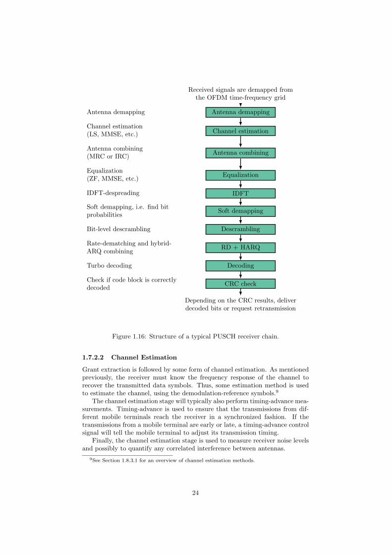
Received signals are demapped fromthe OFDM time-frequency grid

Antenna demapping Antenna demapping

Channel estimation(LS, MMSE, etc.) Channel estimation

Antenna combining(MRC or IRC)

Antenna combining

Equalization(ZF, MMSE, etc.)

Equalization

IDFT-despreading IDFT

Soft demapping, i.e. find bitprobabilities

Soft demapping

Bit-level descrambling Descrambling

Rate-dematching and hybrid-ARQ combining

RD + HARQ

Turbo decoding Decoding

Check if code block is correctlydecoded

CRC check

Depending on the CRC results, deliverdecoded bits or request retransmission

Figure 1.16: Structure of a typical PUSCH receiver chain.

1.7.2.2 Channel Estimation

Grant extraction is followed by some form of channel estimation. As mentionedpreviously, the receiver must know the frequency response of the channel torecover the transmitted data symbols. Thus, some estimation method is usedto estimate the channel, using the demodulation-reference symbols.9

The channel estimation stage will typically also perform timing-advance mea-surements. Timing-advance is used to ensure that the transmissions from dif-ferent mobile terminals reach the receiver in a synchronized fashion. If thetransmissions from a mobile terminal are early or late, a timing-advance controlsignal will tell the mobile terminal to adjust its transmission timing.

Finally, the channel estimation stage is used to measure receiver noise levelsand possibly to quantify any correlated interference between antennas.

9See Section 1.8.3.1 for an overview of channel estimation methods.

24

1.7.2.3 Antenna Combining and Equalization

So far, different receiving antennas have been processed separately. Now thesymbols from different antennas will be combined. This typically done usingMRC or IRC.

Since the transmitted symbols might have been corrupted by a frequency-selective channel, equalization is necessary. For LTE uplink, the MMSE frequency-domain equalizer is an attractive option, for its simplicity and relatively goodperformance.

1.7.2.4 IDFT Despreading

Antenna combining and equalization is followed by a size-M IDFT, to reversethe transmitter-side DFT spreading.

1.7.2.5 Soft Demapping

The purpose of demapping is to recover the transmitted bits from the receivedsymbols. A soft demapper does not take hard decisions on the received symbols,but instead outputs bit likelihoods. The bit likelihoods will depend on both thevalue of the received symbol and the receiver noise levels.

1.7.2.6 Descrambling

Descrambling simply undoes the transmitter-side scrambling, by inverting bitprobabilities where applicable, as given by the scrambling sequence.

1.7.2.7 Rate Dematching and Hybrid-ARQ

Rate dematching is performed to undo the transmitter-side rate matching. ForHARQ, this step tracks any previous transmission and performs maximum ratiocombining when needed.

1.7.2.8 Turbo Decoding

The receiver typically only performs a few iterations of turbo decoding. Thecode-block or transport-block CRC checksum indicates if the decoding has beensuccessful or if a retransmission should be requested.

1.8 Turbo Receivers

This section will introduce the turbo receiver concept. Essentially, turbo re-ceivers are receivers which employ some sort of iterative, feedback processing.The goal is to reduce the bit error rate while keeping the receiver’s complexitylimited. First, turbo codes will be introduced. Turbo codes were the first typeof iterative receiver structure that saw widespread use and they will serve asan introduction to the turbo concept. Turbo codes are also the coding schemeused for forward error correction in LTE. Then, turbo equalization and iterativechannel estimation (ICE) will be introduced.

25

+ +

+ z−1 z−1 z−1

+

Interleaver

+ +

+ z−1 z−1 z−1

+

xk

zk

ck

z′k

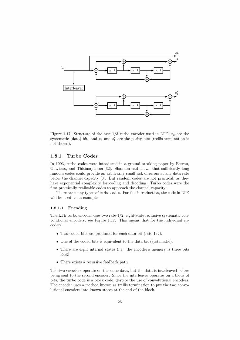
Figure 1.17: Structure of the rate 1/3 turbo encoder used in LTE. xk are thesystematic (data) bits and zk and z′k are the parity bits (trellis termination isnot shown).

1.8.1 Turbo Codes

In 1993, turbo codes were introduced in a ground-breaking paper by Berrou,Glavieux, and Thitimajshima [32]. Shannon had shown that sufficiently longrandom codes could provide an arbitrarily small risk of errors at any data ratebelow the channel capacity [8]. But random codes are not practical, as theyhave exponential complexity for coding and decoding. Turbo codes were thefirst practically realizable codes to approach the channel capacity.

There are many types of turbo codes. For this introduction, the code in LTEwill be used as an example.

1.8.1.1 Encoding

The LTE turbo encoder uses two rate-1/2, eight-state recursive systematic con-volutional encoders, see Figure 1.17. This means that for the individual en-coders:

• Two coded bits are produced for each data bit (rate-1/2).

• One of the coded bits is equivalent to the data bit (systematic).

• There are eight internal states (i.e. the encoder’s memory is three bitslong).

• There exists a recursive feedback path.

The two encoders operate on the same data, but the data is interleaved beforebeing sent to the second encoder. Since the interleaver operates on a block ofbits, the turbo code is a block code, despite the use of convolutional encoders.The encoder uses a method known as trellis termination to put the two convo-lutional encoders into known states at the end of the block.

26

1.8.1.2 Decoding

To decode a signal protected by a turbo code, a soft demapper is used to cal-culate bit-likelihoods. A bit likelihood is the probability that a given bit is zero(or, equivalently, that a given bit is one). The bit-likelihoods are a function ofthe received symbol and the channel noise level.

These likelihoods are known as a-priory likelihoods, since they only considerthe received signal and not the structure of the code. The optimal decodingstrategy would be to find the maximum a-posterior (MAP) solution, that is,the most likely sequence of data bits given the received signal and the codestructure. But doing this for the whole code is computationally infeasible, asthe total number of states is too high.

However, for each separate encoder, there are relatively few states, and aMAP algorithm is feasible on a per-encoder basis. An algorithm similar to thebackwards-forwards algorithm used for hidden Markov models, known as theBJCR algorithm, can be used to find the MAP likelihoods [33]. The BJCRalgorithm is often used in its simplified Log-MAP form [34]. As the algorithmconsiders each encoder separately, it will only find local optimums, not the MAPsolution for the whole code structure.

The difference between the a-priory and the a-posterior probabilities is knownas the extrinsic information, which can be seen as the information gained fromthe use each separate encoder.

Having first performed one round of MAP decoding for each of the two con-stituent encoders, the decoders exchanges extrinsic information with each other.The extrinsic information is then used to modify the a-priory bit likelihoods.Due to the interleaver, errors will be statistically independent between the twodecoders.

It is this iterative exchange of information that forms the “turbo” part of thecode. The decoding process is not guaranteed to provide the same performanceas if MAP decoding had been used for both constituent encoders simultaneously,but in practice, the method provides very good performance.

1.8.2 Turbo Equalization

Turbo equalization extends the turbo concept to channel equalization. Whereturbo codes exchanges information between two constituent decoders, turboequalization exchanges information between the channel equalizer and the turbodecoder.

This section will first show why inter-symbol inference (ISI) appears inDFTS-OFDM systems and then how turbo equalization can be used to coun-teract the interference.

1.8.2.1 Inter-Symbol Interference in DFTS-OFDM Systems

Consider a sequence s sent with DFT-spreading over an OFDM modulatedchannel with impulse response g (which is assumed to be short enough for thecyclic prefix to prevent inter-block interference). The received frequency-domainsignal is

y = F (g)⊗F (s) + F (n)

27

where ⊗ denotes the element-wise product. To recover s, the receiver needs toreverse the DFT-spreading. The naıve approach gives

F−1 (y) = F−1(F (g)⊗F (s)) + n

F−1 (y) = g ∗ s + n

where the last equality uses the convolution theorem. The term g∗s means thatthe transmitted symbols will be convolved with the channels impulse response,resulting in inter-symbol interference within a block. This inter-symbol canbe completely removed by zero-forcing equalization, but this give unreasonablenoise enhancement. MMSE equalization typically gives a good trade-off be-tween noise enhancement and inter-symbol interference suppression, but cannotcompletely remove the interference.

1.8.2.2 Turbo Equalization for Interference Cancellation

Turbo equalization provides a third alternative, where regenerated symbols arefeed back to the equalizer [35]. By knowing what the interfering symbols are, theequalizer can cancel the interference. The equalizer and the decoder togetherform a turbo loop. The equalizer tries to remove the effects of a selectivechannel, which helps the decoder. The decoder provides the equalizer withestimated symbols, which improves the equalizer.

Since decoded symbols are fed back, turbo equalization is a form of decisionfeedback equalization.

1.8.3 Iterative Channel Estimation

This section will first review how channel estimation typically is performed inOFDM systems and then how iterative channel estimation can improve thechannel estimate in LTE uplink.

1.8.3.1 Channel Estimation in OFDM Systems

Two well-known channel estimation techniques are LS and MMSE [36]. Thesetwo estimators are similar to the ZF and MMSE equalization concepts, seesection 1.4.1. The LS channel estimate for subcarrier k in an OFDM system is

hk =ykxk

where y is the received symbol and x is the transmitted symbol.10 For theeMMSE channel estimation proposed in [36], the channel impulse response ismodeled as a complex Gaussian vector

g = CN (0,Rgg)

and the MMSE channel estimate is

h = FQMMSEFHXHy

10Compare this expression with equation (1.1).

28

where F is the DFT-matrix, X = diag (x) and

QMMSE = Rgg

(FHXHXFσ2

n + Rgg

)−1 (FHXHXF

)−1

Both estimators have advantages and disadvantages. The LS estimator hasvery low complexity, but will tend to amplify noise at frequencies where thetransmitted symbol has low energy. Further, the LS estimator does not con-sider the correlation between channel taps, which is usually strong. The MMSEestimator on the other hand is the best linear estimator in a least-square er-ror sense. But it requires knowledge of the channel covariance matrix and theinversion of an NSC ×NSC matrix. The complexity can be reduced by only ac-counting for the first L channel taps, known as approximate MMSE (AMMSE),which reduces the size of the inversion to an L×L matrix, at the cost of reducedperformance, especially at high SNR.

1.8.3.2 Problems With Pilot-Based Channel Estimation

The channel estimation methods described above require that the transmittedsymbols x are known. This is called pilot-based channel estimation, since specialpilot symbols are inserted into the transmitted signal for the purpose of channelestimation. In LTE, the DM-RS are the pilot symbols.

Use of pilot symbols involves a trade-off. The energy available to estimatethe channel is proportional to the density of pilot symbols, and more energygives lower noise in the channel estimate. But each pilot symbol displaces adata symbol, decreasing the effective data rate.

A further consideration is one of sampling. In LTE uplink, the spacingof the DM-RS is about 0.5 ms. This means that, by the sampling theorem,channel variations faster than 1000 Hz (corresponding to a speed of 500 km/hfor a 2 GHz carrier) can not be resolved. In practice, channels will very rarelyvary so fast, but the sampling theorem is only fully applicable for infinitely longsignals. In LTE, sometimes only a single subframe may be available to estimatethe channel. With only two samples of the channel, one from each DM-RS inthe subframe, the problem of reconstruction the channel’s time variations isunder-determined, even with the assumption that the variations are limited tobelow the Nyquist frequency.

1.8.3.3 Iterative Channel Estimation as a Solution

Iterative channel estimation tries to relieve some of these problems. First, thepilot symbols are used to estimate the channel. The received data symbols arethen equalized, using the channel estimate. In addition to receiver noise, theequalized data symbols will be corrupted by errors in the channel estimate. Thetransmitted data bits are protected by an error correcting code, so a decoderis used to correct some of the errors introduced by receiver noise and channelestimation errors. Typically, the data bits are protected by some addition errordetection coding. If an error is detected in the decoded bits, the bits are re-encoded to regenerate the transmitted symbols. The regenerated symbols arethen feed back to the channel estimation stage, where they are treated as aadditional set of pilot symbols and the whole receiver process repeats.

29

This feedback has two effects. Firstly, the power available for channel es-timation increases, decreasing the impact of noise. Secondly, it increases theeffective sampling rate, improving the tracking of a time-varying channel.

Iterative channel estimation can be used in conjecture with turbo equaliza-tion, with the turbo equalizer forming a loop inside the ICE loop.

1.8.3.4 Previous Work

Different types of ICE have been suggested. For example, [37] and [38] sug-gested methods with soft feedback (i.e. bit likelihoods are fed back). [39] usedthe recursive least-squares algorithm together with soft feedback to track atime-varying channel, extending the idea in [40]. [41] used two cascaded one-dimensional Wiener filters to interpolate the channel estimate. [42] used a mov-ing average to estimate time-varying channels, pointing out the need to considerthe reliability of the soft feedback when averaging.

Iterative channel estimation has been applied to LTE downlink. For exam-ple, [43] suggested a simplified iterative method using 2×1D interpolation andweighted averaging of pilot and data based channel estimates. Later, [44] usedsoft feedback together with LS, MMSE and AMMSE channel estimation.

ICE has been shown to be a promising technique for improving channelestimation. But to the author’s knowledge, no one has applied ICE to LTEuplink. Use of ICE in uplink might be more feasible than use in downlink, asbase stations typically have more processing power than mobile terminals. Buteven so, the complexity of an ICE algorithm must be low if it is to be used inreal-world systems. Fortunately, several of the papers cited above reports goodperformance even with low-complexity estimators.

30

Chapter 2

Methods

This chapter will describe the specific methods used in this thesis. The firstpart will propose an algorithm for ICE. This is followed by a description of theturbo equalization algorithm used, the other components of the receiver chainand the different channel models used for simulations. Figure 2.1 shows how theiterative channel estimation and turbo equalization feedback loops will operatein the receiver.

Antenna demapping

Channel estimation

Antenna combining

Equalizer

IDFT

Soft demapper

Turbo decoder

CRC check? Soft mapper

DFT

Fail

Pass

Turbo equilization

Iterative channelestimation

Figure 2.1: Illustration of how the iterative channel estimation and turbo equal-ization uses regenerated symbols as feedback.

31

2.1 Iterative Channel Estimator

This section will first present the requirements for an ICE algorithm, includ-ing the restrictions, i.e. what the algorithm not is expected to do. Then theproposed algorithm will be described.

2.1.1 Requirements

The guiding principle for the requirements was to design an algorithm that ispractically realizable in a real system. This immediately led to some require-ments. The algorithm should:

• Operate with limited knowledge of the channel. This means that the re-ceiver noise variance is unknown. It also means that any channel statisticsis unknown.

• Estimate the receiver noise variance. This value is needed by other stagesof the receiver chain, for example the equalizer and the soft demapper,and should be provided by the channel estimator.

• Operate with limited complexity. The computational complexity mustgrow at a reasonably rate with the number of subcarriers.

• Operate on only the demodulation-reference signals when necessary, sothe same algorithm can be used for the initial channel estimation.

In addition to the above requirements, the algorithm should also generalize tothe MIMO case.

The requirement for limited channel knowledge means that conventionalMMSE channel estimation is not possible, since MMSE channel estimation re-quires knowledge of the channel’s auto-covariance matrix. The auto-covariancecould be estimated by averaging across subframes, but this is not a realizablesolution since the scheduler can potentially assign users different subcarriers foreach subframe.

Limited computational complexity is a somewhat vague requirement. Basestations have very specialized hardware. Typically, they have a large num-ber of digital signal processors (DSP) that operates in parallel. They also oftenhave very fast application-specific integrated circuits (ASIC) for performing fastFourier transforms. Thus, the complexity of an algorithm cannot be measuredonly by the number of operations needed, but also by how well it can be paral-lelized and if it can make use of dedicated circuitry.

2.1.1.1 Restrictions

Some functions typically performed by a receiver’s channel estimation stagewere excluded from the requirements. Specifically, it is assumed that there areno timing advance errors and no frequency offsets.

These two restrictions were imposed to limit the number of cases that neededto be tested when evaluating performance, and being deemed unimportant whenevaluating the gains of iterative channel estimation.

Timing advance errors do not directly affect the channel estimation, but thechannel estimation stage should provide timing advance measurements for the

32

scheduler to use. This is typically done by measuring at what time delay mostof the received signal’s energy is concentrated.

Frequency offset errors arise from the radial velocity of the remote device(Doppler shift). They can also be the result of errors in the frequency of theremote device’s and/or the base station’s local oscillator. Frequency offsets ap-pear as a complex rotation of the channel coefficients. Measuring the frequencyoffset typically requires averaging across several subframes, which the channelestimation algorithm will not do. However, the channel estimation algorithmdescription below includes compensation for a known frequency offset.

2.1.2 Conventions

The following conventions are used. The frequency domain system model isgiven by

ynr,m,k =

NT−1∑

nt=0

hnt,nr,m,kxnt,m,k + nnr,m,k (2.1)

where y is the received signal, h is the channel coefficient, x is the transmittedsymbol, n is white Gaussian noise with variance σ2

n and nt, nr, m, k are theindexes for the transmit antenna, the receive antenna, the OFDM symbol andthe subcarrier. NT is the number of transmit antennas.

The symbols are either demodulation reference symbols

m ∈ P = {3, 10}

or data symbols1

m ∈ D = {0, 1, . . . , 13} \ PThe data symbols are modeled as a zero mean Gaussian variables with vari-

ance σ2x = 1. This approximation is motivated by the central limit theorem.

Before DFT-spreading, the symbols are drawn from some of the LTE modu-lations alphabets and are thus clearly not Gaussian. But the DFT-spreadingoperations means that each transmitted symbol is a linear combination of multi-ple independent symbols (by the assumption that the transmitted data bits areuncorrelated with each other). Thus, the transmitted symbols can be approxi-mated as Gaussian. The data symbols prior to DFT-spreading will be referredto as time-domain symbols and the data symbols after DFT-spreading will bereferred to as frequency-domain symbols.

2.1.3 Proposed Algorithm

This section will propose an ICE algorithm. The algorithm has several modularcomponents and in some cases different sub-algorithms were tested. Refer toFigure 2.2 for an overview of the algorithm.

The algorithm always operates on single subframes. In general, the stepsare as follows:

1. Any decoded data that might be available is used to reconstruct the trans-mitted signal. If no decoded data is available, only the DM-RS signals areused.

1P = {2, 8} and D = {0, 1, . . . , 11} \ P in the case of extended cyclic prefix.

33

Symbol regeneration

Variance/covarianceestimation

Interferencecancellation

Point-wise channelcoefficient estimation

Frequency offsetcompensation

Model fittingChannel length

estimation

Model selection

Channel filtering

Channel regeneration

Frequency offsetuncompensation

All paths estimated?

Noise estimation

If decoded bitsare available

Per

RX

ante

nn

a

Per

TX

ante

nn

a

σ2LS

Lopt

Yes

No

Cancel contribution from pre-viously estimated path (SIC)

Figure 2.2: Flow of the proposed ICE algorithm. This figure corresponds to thesoft mapper, DFT and channel estimation block in Figure 2.1.

34

2. A point-wise estimate is made of the channel, similar to the LS estimatedescribed in Section 1.8.3.1. This estimate is unbiased, but very noise.

3. A low-order polynomial model is fitted to the point-wise estimates for eachsubcarrier. This suppresses much of the noise present in the point-wiseestimate.

4. The polynomial model is filtered. While the polynomial model is a rea-sonable approximation of the time variations of a single subcarrier, thepolynomial fitting does not take into account the (usually strong) cor-relation between subcarriers. This is handled by applying an adaptivelow-pass filter to the polynomial coefficients for all subcarriers.

These are just are the main parts of the proposed algorithm. The followingsections will explain the entire algorithm in detail.

2.1.3.1 Symbol Regeneration

For the demodulation-reference symbols, no actual regeneration is necessary,since the reference sequences are known. For the first round of the iterativechannel estimation, no data bit-likelihoods are available and data symbol re-generation is skipped. But for subsequent estimation iterations, data symbolregeneration is needed. This is done by soft mapper which takes bit likelihoodsfrom the turbo decoder and regenerates the transmitted symbols. The regen-eration is performed per code block. For notational simplicity, the transmitterindex is dropped.

As is common, the turbo decoder is assumed to output bit log-likelihoodratios, defined as

fn = ln

(P(bnbm,n = 1

)

P (bnbm,n = 0)

)

where bnbm,n is the nb:th bit of the time-domain symbol transmitted at OFDMsymbol m and at sample n.

The estimate of the time-domain data symbols is taken as

sm,n = E{sm,n | f0

m,n, f1m,n, . . . , f

NC−1m,n

}

where sm,n is the estimated data symbol and NC is the number of bits persymbol. The expected value is given by

sm,n =

M−1∑

i=0

(ai

NC−1∏

nb=0

P(fnbm,n, ai

))

where M = 2NC is the number of symbols in the constellation, ai is the i:thsymbol of the constellation and P

(fnbm,n, ai

)is the probability that bit nb cor-

responds to the value associated with the symbol ai.The regenerated symbols for different modulation schemes can be expressed

explicitly as2

2This follows from the Gray mappings defined in [10].

35

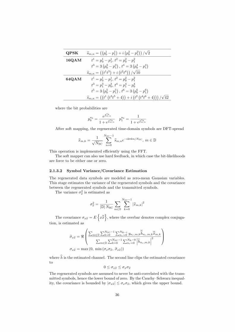
QPSK sm,n =((p1

0 − p11

)+ i(p2

0 − p21

))/√

2

16QAM t1 = p10 − p1

1, t2 = p20 − p2

1

t3 = 3(p3

0 − p31

), t4 = 3

(p4

0 − p41

)

sm,n =((t1t3

)+ i(t2t4

))/√

10

64QAM t1 = p10 − p1

1, t2 = p20 − p2

1

t3 = p31 − p3

0, t4 = p41 − p4

0

t5 = 3(p5

0 − p51

), t6 = 3

(p6

0 − p61

)

sm,n =((t1(t3t5 + 4

))+ i(t2(t4t6 + 4

)))/√

42

where the bit probabilities are

pnb0 =ef

nbm,n

1 + efnbm,n

pnb1 =1

1 + efnbm,n

After soft mapping, the regenerated time-domain symbols are DFT-spread

xm,k =1√NSC

NSC−1∑

n=0

sm,ne−i2πkn/NSC , m ∈ D

This operation is implemented efficiently using the FFT.The soft mapper can also use hard feedback, in which case the bit-likelihoods

are force to be either one or zero.

2.1.3.2 Symbol Variance/Covariance Estimation

The regenerated data symbols are modeled as zero-mean Gaussian variables.This stage estimates the variance of the regenerated symbols and the covariancebetween the regenerated symbols and the transmitted symbols.

The variance σ2x is estimated as

σ2x =

1

|D|NSC

∑

m∈D

NSC−1∑

k=0

|xm,k|2

The covariance σxx = E{xx}

, where the overbar denotes complex conjuga-

tion, is estimated as

σxx = <

∑m∈D

∑NSC−1k=0

∑NR−1

nr=0 ynr,m,khnr,m,kxm,k∑m∈D

∑NSC−1k=0

∑NR−0nr=0

∣∣∣hnr,m,k∣∣∣2

σxx = max (0, min (σxσx, σxx))

where h is the estimated channel. The second line clips the estimated covarianceto

0 ≤ σxx ≤ σxσxThe regenerated symbols are assumed to never be anti-correlated with the trans-mitted symbols, hence the lower bound of zero. By the Cauchy–Schwarz inequal-ity, the covariance is bounded by |σxx| ≤ σxσx, which gives the upper bound.

36

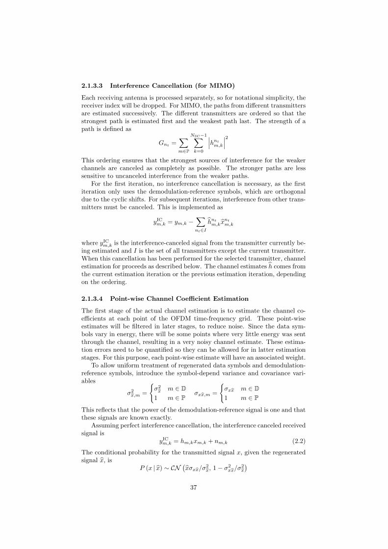
2.1.3.3 Interference Cancellation (for MIMO)

Each receiving antenna is processed separately, so for notational simplicity, thereceiver index will be dropped. For MIMO, the paths from different transmittersare estimated successively. The different transmitters are ordered so that thestrongest path is estimated first and the weakest path last. The strength of apath is defined as

Gnt =∑

m∈P

NSC−1∑

k=0

∣∣∣hntm,k∣∣∣2

This ordering ensures that the strongest sources of interference for the weakerchannels are canceled as completely as possible. The stronger paths are lesssensitive to uncanceled interference from the weaker paths.

For the first iteration, no interference cancellation is necessary, as the firstiteration only uses the demodulation-reference symbols, which are orthogonaldue to the cyclic shifts. For subsequent iterations, interference from other trans-mitters must be canceled. This is implemented as

yICm,k = ym,k −

∑

nt∈Ihntm,kx

ntm,k

where yICm,k is the interference-canceled signal from the transmitter currently be-

ing estimated and I is the set of all transmitters except the current transmitter.When this cancellation has been performed for the selected transmitter, channelestimation for proceeds as described below. The channel estimates h comes fromthe current estimation iteration or the previous estimation iteration, dependingon the ordering.

2.1.3.4 Point-wise Channel Coefficient Estimation

The first stage of the actual channel estimation is to estimate the channel co-efficients at each point of the OFDM time-frequency grid. These point-wiseestimates will be filtered in later stages, to reduce noise. Since the data sym-bols vary in energy, there will be some points where very little energy was sentthrough the channel, resulting in a very noisy channel estimate. These estima-tion errors need to be quantified so they can be allowed for in latter estimationstages. For this purpose, each point-wise estimate will have an associated weight.

To allow uniform treatment of regenerated data symbols and demodulation-reference symbols, introduce the symbol-depend variance and covariance vari-ables

σ2x,m =

{σ2x m ∈ D

1 m ∈ Pσxx,m =

{σxx m ∈ D1 m ∈ P

This reflects that the power of the demodulation-reference signal is one and thatthese signals are known exactly.

Assuming perfect interference cancellation, the interference canceled receivedsignal is

yICm,k = hm,kxm,k + nm,k (2.2)

The conditional probability for the transmitted signal x, given the regeneratedsignal x, is

P (x | x) ∼ CN(xσxx/σ

2x, 1− σ2

xx/σ2x

)

37

Thus, equation (2.2) can be rewritten as

yICm,k = hm,k(xm,kσxx,m/σ

2x,m + xm,k) + nm,k (2.3)

wherex ∼ N

(0, 1− σ2

xx,m/σ2x,m

)(2.4)

and E {xx} = 0. From (2.3) and (2.4), it can be seen that an unbiased estimateof h is

hLSm,k = yIC

m,k/(xm,kσxx,m/σ

2x,m

)(2.5)

The variance of the estimation error is

E

{(hm,k − hLS

m,k

)2}

=|hm,k|2

(1− σ2

xx,m/σ2x,m

)+ σ2

n

(|xm,k|σxx,m/σ2

x,m

)2

For any iteration, the point-wise channel estimate is given by expression(2.5). For the demodulation-reference symbols, σxx,m/σ

2x,m = 1, the expression

can be evaluate even if only demodulation-reference signals are available. Fig-ure 2.4 illustrates this point-wise estimation applied to the channel depicted inFigure 2.3.

The weight of an estimate should be proportional to the inverse of the errorvariance, and is taken as

wLSm,k =

(|xm,k|σxx,m/σ2

x,m

)2

|hm,k|2σ2n

(1− σ2

xx,m/σ2x,m

)+ 1

Here the inverse variance has been scaled by σ2n, to make the weights equal to

one for the demodulation-reference symbols.A simplified method of this least-squares channel estimation was also imple-

mented. In this case, it was assumed that

σxx = σx

This removes the need to estimate the regenerated symbol covariance and sim-plifies the point-wise channel estimate and weight calculation

hLSm,k =

yICm,k

xm,k/σx,m

wLSm,k = (|xm,k| /σx,m)

2

A further simplification was also tested, which assumed

σ2x = 1

This removes the need to estimate σ2x and further simplifies the point-wise esti-

mate and weight calculation

hLSm,k =

yICm,k

xm,k

wLSm,k = |xm,k|2

38

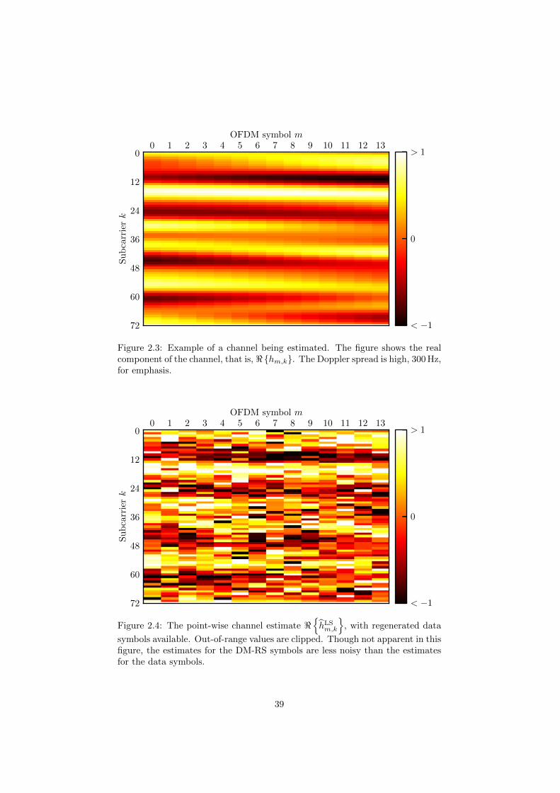
0 1 2 3 4 5 6 7 8 9 10 11 12 13OFDM symbol m

0

12

24

36

48

60

72

Su

bca

rrie

rk

< −1

0

> 1

Figure 2.3: Example of a channel being estimated. The figure shows the realcomponent of the channel, that is, <{hm,k}. The Doppler spread is high, 300 Hz,for emphasis.

0 1 2 3 4 5 6 7 8 9 10 11 12 13OFDM symbol m

0

12

24

36

48

60

72

Su

bca

rrie

rk

< −1

0

> 1

Figure 2.4: The point-wise channel estimate <{hLSm,k

}, with regenerated data

symbols available. Out-of-range values are clipped. Though not apparent in thisfigure, the estimates for the DM-RS symbols are less noisy than the estimatesfor the data symbols.

39

2.1.3.5 Frequency Offset Compensation

Any frequency offset will have a detrimental effect on the later model fittingand model selection stages. Therefore, the frequency offset is compensated forby rotating the channel estimate

hLS,compm,k = hLS

m,ke2πi4τmfoffset

where 4τ is the time between successive symbols and foffset is the frequencyoffset.

2.1.3.6 Model Fitting

It is assumed that the channel for any given subcarrier can be modeled as apolynomial

hm,k =

ν−1∑

q=0

bνq,k · g (m)q

where bνq,k is the q:th polynomial coefficient for the k:th subcarrier, for a poly-nomial of order ν. The polynomial order ν is 0, 1 or 2. The function g(·) isdefined as

g (m) =2

NS − 1m− 1

where NS is the number of OFDM symbols in a subframe.This construction implies that each subcarrier is modeled as a ν:th order

polynomial across OFDM symbols. The model order ν is shared across allsubcarriers. This model was selected for its simplicity, compared to, for example,basis-expansion models [45]. By using g(·) instead of the OFDM symbol indexdirectly, the polynomial coefficients becomes less depended on the number ofOFDM symbols per subframe. This is important for the latter model selectionstage.

Introduce the set of available symbols

S =

{D ∪ P if regenerated data symbols are availabe

P otherwise

and let bνk =[bν0,k, b

ν1,k, . . . , b

νν−1,k

]. The coefficient vector bνk is selected to

minimize the weighted sum of square errors

bνk = arg minbνk

∑

m∈S

∣∣∣∣∣hLS,compm,k −

ν−1∑

q=0

bνq,k · g (m)q

∣∣∣∣∣

2

wLSm,k

In matrix notation, the minimization problem can be expressed as

bνk = arg minbνk

((hk −Vνbνk)

TWk (hk −Vνbνk)

)

40

where

Vν =

1 g(S0) · · · g(S0)ν−1

1 g(S1) · · · g(S1)ν−1

......

. . ....

1 g(S|S|−1) · · · g(S|S|−1)ν−1

Wk = diag([wLS

S0,k, wLSS1,k, . . . , w

LSS|S|−1,k

])

hk =[hLS,compS0,k , hLS,comp

S1,k , . . . , hLS,compS|S|−1,k

]T

The solution is

bνk =(VνTWkV

ν)−1

VνTWkhk

This fitting is performed for a constant and a linear model (ν = 0 and 1).These calculations can be simplified to

b00,k =

∑m∈S h

LS,compm,k wLS

m,k∑m∈S w

LSm,k

b

10,k

b11,k

=

∑m∈S w

LSm,k

∑m∈S g(m)wLS

m,k∑m∈S g(m)wLS

m,k

∑m∈S g(m)2wLS

m,k

−1

∑m∈S h

LS,compm,k wLS

m,k∑m∈S g(m)hLS,comp

m,k wLSm,k

Note that the two equations share some coefficients. This can be used to speedup the computations.

2.1.3.7 Channel Length Estimation

This stage estimates the length of the channel impulse response. It will alsoestimate how noisy the channel estimate is.

The channel length is estimated in the discrete cosine transform (DCT)domain, using a heuristic criterion. It might seem counter intuitive to performthe channel length estimation in the DCT-domain instead of the time-domain,but this works well together with the later channel filtering stage.

First, the constant channel approximation (ν = 0) is transformed to theDCT-domain

dn =

NSC−1∑

k=0

w (k) b00,k cos

(π

NSC

(k +

1

2

)n

)

where

w (k) =

1√NSC

k = 0√

2

NSC1 ≤ k < NSC

The DCT operation can be implemented efficiently using the FFT [46].The residual variance σ2

LS (L), where L is the channel length, is defined as

σ2LS (L) =

1

Nwin

Nwin−1∑

n=L

|dn|2

41

where the window length Nwin is defined as

Nwin = NSC/Nusers

and Nusers is the number of co-scheduled users in a MIMO situation.This limit on the window length is intended to prevent interference between

users for the first iterative estimation stage. The point-wise channel estimationcorresponds to matched filter estimation. As explained in Section 1.6.3, matchedfiltering of a cyclic-shifted DM-RS modulates other users’ channel responses bya complex sinusoidal signal

hotherk e−iπαk

This modulation shifts the other users channel responses to higher frequenciesin the DCT-domain. Assuming that users have been assigned cyclic shifts asto maximize the separation between them, the window length limit will rejectthe majority of the response from other users channels (some inter-modulationproducts may remain).

A heuristic criterion is used to select the optimal channel length Lopt, basedon σ2

LS (L). The estimation noise variance σ2LS is defined as

σ2LS =

Nwin

Nwin − Loptσ2

LS (Lopt)

This corresponds to the average variance outside the channel length and can beseen as a simple measure of the noise affecting the channel estimation.

2.1.3.8 Model Selection

The channel length estimation is followed by a model selection step. A higherorder model will fit a fast varying channel better than a lower order model,but the introduction of extra free parameters makes the model fitting moresusceptible to noise. Model selection tries to use a low-order model when thechannel varies slowly and/or the noise is high and a high-order model when thechannel varies fast and the noise is low.

This is implemented using a switching variable and a set of thresholds. Theswitching variable Θ is defined as

Θ =

NSC−1∑

k=0

∣∣b11,k∣∣2 /σ2

LS

b11,k is the coefficient for the slope of the linear approximation. The optimalmodel order νopt is selected as

νopt =

0 for 0 ≤ Θ ≤ 3.5

1 for 3.5 < Θ ≤ 64

2 otherwise

In addition to the threshold, the second-order model can only be selected ifregenerated data symbols are available; otherwise the least-squares problem isunder-determined. The zeroth and first-order models have already been fitted,but if the second-order model is selected, it needs to be fitted.

The thresholds have been selected by trial-and-error to provide reasonableperformance across different channel and SNR conditions, but are not optimized.

42

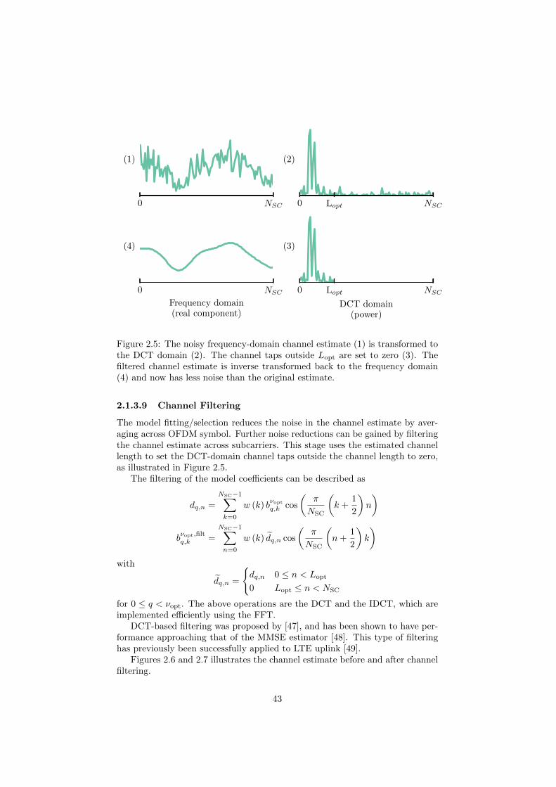
0 NSC

(1)

0 Lopt NSC

(2)

0 Lopt NSC

DCT domain(power)

(3)

0 NSCFrequency domain(real component)

(4)

Figure 2.5: The noisy frequency-domain channel estimate (1) is transformed tothe DCT domain (2). The channel taps outside Lopt are set to zero (3). Thefiltered channel estimate is inverse transformed back to the frequency domain(4) and now has less noise than the original estimate.

2.1.3.9 Channel Filtering

The model fitting/selection reduces the noise in the channel estimate by aver-aging across OFDM symbol. Further noise reductions can be gained by filteringthe channel estimate across subcarriers. This stage uses the estimated channellength to set the DCT-domain channel taps outside the channel length to zero,as illustrated in Figure 2.5.

The filtering of the model coefficients can be described as

dq,n =

NSC−1∑

k=0

w (k) bνoptq,k cos

(π

NSC

(k +

1

2

)n

)

bνopt,filtq,k =

NSC−1∑

n=0

w (k) dq,n cos

(π

NSC

(n+

1

2

)k

)

with

dq,n =

{dq,n 0 ≤ n < Lopt

0 Lopt ≤ n < NSC

for 0 ≤ q < νopt. The above operations are the DCT and the IDCT, which areimplemented efficiently using the FFT.

DCT-based filtering was proposed by [47], and has been shown to have per-formance approaching that of the MMSE estimator [48]. This type of filteringhas previously been successfully applied to LTE uplink [49].

Figures 2.6 and 2.7 illustrates the channel estimate before and after channelfiltering.

43

0 1 2 3 4 5 6 7 8 9 10 11 12 13OFDM symbol m

0

12

24

36

48

60

72

Su

bca

rrie

rk

< −1

0

> 1

Figure 2.6: The estimated channel after model selection. In this case, eachsubcarrier is modeled as a first-order polynomial. Note how there is some high-frequency noise along the y-axis, compared to the real channel (see Figure 2.3).

0 1 2 3 4 5 6 7 8 9 10 11 12 13OFDM symbol m

0

12

24

36

48

60

72

Su

bca

rrie

rk

< −1

0

> 1

Figure 2.7: The estimated channel after channel filtering, that is, <{hm,k

}.

Note how the high-frequency noise present in Figure 2.6 has been suppressed.

44

2.1.3.10 Channel Regeneration

When the filtering is complete, a channel estimate is generated from the modelcoefficients for each point on the OFDM time-frequency grid

hfiltm,k =

νopt−1∑

q=0

bνopt,filtq,k · g (m)

q

2.1.3.11 Frequency Offset Uncompensation

Finally, the frequency offset compensation is reversed

hm,k = hfiltm,ke

−2πi4τmfoffset

This gives the final channel estimate.

2.1.3.12 Noise Estimation

Noise estimation aims to measure the receiver noise at each antenna. This isperformed first when the paths from all transmitters have been estimated forthe receiving antenna. The noise variance is estimated as3

σ2n =

1

|P|NSC

∑

m∈P

NSC−1∑

k=0

∣∣∣∣∣ym,k −NT−1∑

nt=0

hntm,kxntm,k

∣∣∣∣∣

2

Since only the demodulation-reference symbols are used, this expression can beevaluated even when there are no regenerated data symbols.

2.2 Turbo Equalizer

The turbo equalization algorithm is essentially the same method as describedin [50], with the adaptive coefficients described in [51]. Since the receiver chainperforms maximal ratio combining as a separate stage from equalization, theturbo equalization algorithm operates as if there is only one receiving antenna,with channel taps and noise variance derived from the combining stage. As in[51], the full a-posterior bit-likelihoods are used, without any modification tothe soft mapper. In fact, the turbo equalizer shares the soft mapper with theiterative channel estimator.

2.3 Other Receiver Components

The receiver uses MRC to combine the received symbols from multiple receivingantennas. The combined symbols are equalized using an MMSE equalizer (whenthe turbo equalizer is not used). This is followed by soft demapping, as describedin [52]. The turbo decoder performs up to 8 iterations of decoding.

3Compare this expression to equation (2.1).

45

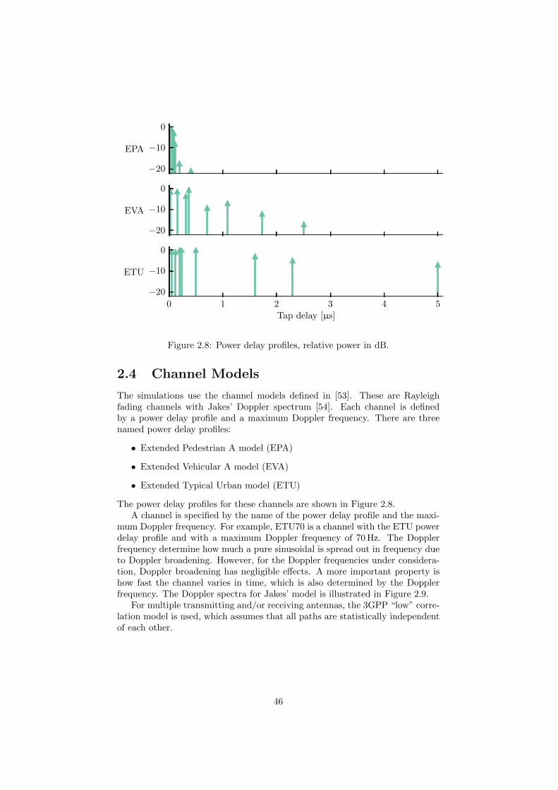
−20

−10

0

EPA

−20

−10

0

EVA

0 1 2 3 4 5

Tap delay [µs]

−20

−10

0

ETU

Figure 2.8: Power delay profiles, relative power in dB.

2.4 Channel Models

The simulations use the channel models defined in [53]. These are Rayleighfading channels with Jakes’ Doppler spectrum [54]. Each channel is definedby a power delay profile and a maximum Doppler frequency. There are threenamed power delay profiles:

• Extended Pedestrian A model (EPA)

• Extended Vehicular A model (EVA)

• Extended Typical Urban model (ETU)

The power delay profiles for these channels are shown in Figure 2.8.A channel is specified by the name of the power delay profile and the maxi-

mum Doppler frequency. For example, ETU70 is a channel with the ETU powerdelay profile and with a maximum Doppler frequency of 70 Hz. The Dopplerfrequency determine how much a pure sinusoidal is spread out in frequency dueto Doppler broadening. However, for the Doppler frequencies under considera-tion, Doppler broadening has negligible effects. A more important property ishow fast the channel varies in time, which is also determined by the Dopplerfrequency. The Doppler spectra for Jakes’ model is illustrated in Figure 2.9.

For multiple transmitting and/or receiving antennas, the 3GPP “low” corre-lation model is used, which assumes that all paths are statistically independentof each other.

46

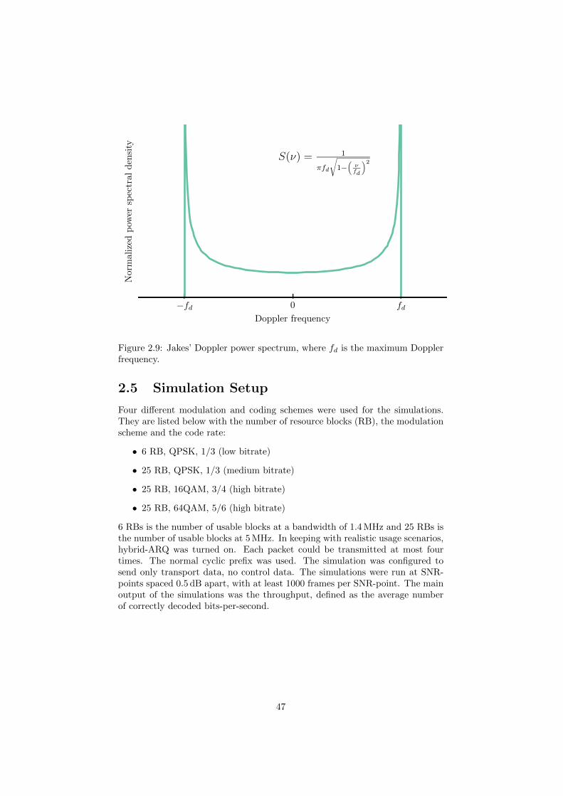
−fd 0 fdDoppler frequency

Nor

mal

ized

pow

ersp

ectr

ald

ensi

ty

S(ν) = 1

πfd

√1−(νfd

)2

Figure 2.9: Jakes’ Doppler power spectrum, where fd is the maximum Dopplerfrequency.

2.5 Simulation Setup

Four different modulation and coding schemes were used for the simulations.They are listed below with the number of resource blocks (RB), the modulationscheme and the code rate:

• 6 RB, QPSK, 1/3 (low bitrate)

• 25 RB, QPSK, 1/3 (medium bitrate)

• 25 RB, 16QAM, 3/4 (high bitrate)

• 25 RB, 64QAM, 5/6 (high bitrate)

6 RBs is the number of usable blocks at a bandwidth of 1.4 MHz and 25 RBs isthe number of usable blocks at 5 MHz. In keeping with realistic usage scenarios,hybrid-ARQ was turned on. Each packet could be transmitted at most fourtimes. The normal cyclic prefix was used. The simulation was configured tosend only transport data, no control data. The simulations were run at SNR-points spaced 0.5 dB apart, with at least 1000 frames per SNR-point. The mainoutput of the simulations was the throughput, defined as the average numberof correctly decoded bits-per-second.

47

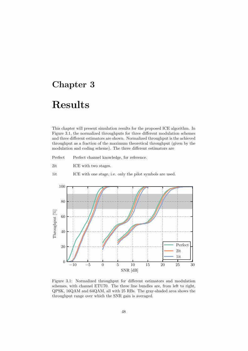
Chapter 3

Results

This chapter will present simulation results for the proposed ICE algorithm. InFigure 3.1, the normalized throughputs for three different modulation schemesand three different estimators are shown. Normalized throughput is the achievedthroughput as a fraction of the maximum theoretical throughput (given by themodulation and coding scheme). The three different estimators are

Perfect Perfect channel knowledge, for reference.

2it ICE with two stages.

1it ICE with one stage, i.e. only the pilot symbols are used.

−10 −5 0 5 10 15 20 25 30

SNR [dB]

0

20

40

60

80

100

Th

rou

ghp

ut

[%]

Perfect

2it

1it

Figure 3.1: Normalized throughput for different estimators and modulationschemes, with channel ETU70. The three line bundles are, from left to right,QPSK, 16QAM and 64QAM, all with 25 RBs. The gray-shaded area shows thethroughput range over which the SNR gain is averaged.

48

9 10 11 12 13 14

SNR [dB]

60

80

100T

hro

ugh

pu

t[%

]

0.6 dB

0.6 dB

0.7 dB

0.7 dB

2it

1it

Figure 3.2: Example of how the SNR gain is defined. Each black arrow showsthe SNR gain of the two stage estimator, relative the one stage estimator, at aspecific throughput.

In keeping with common practice, the performance will be measured in termsof SNR gain, as illustrated in Figure 3.2. With any method, a certain SNRis needed to achieve a specific throughput. The required SNR will differ fordifferent methods. The SNR gain of a method is the difference in SNR neededby that method and the SNR needed by a reference method. The SNR gaincorresponds to an increase in cell size or, equivalently, a reduction in transmitterpower usage.

To make the results easier to interpret, the SNR gain has been average overa normalized throughput range from 70 % to 90 %. This range is shown as agray-shaded area in Figure 3.1. Since the simulations specify the working pointin terms of SNR, as opposed to throughput, the SNR for a given throughputcannot be found directly. To average the SNR over the chosen throughput range,linear interpolation is used.

The 6 RB QPSK and the 25 RB QPSK results are similar, so for clarity onlythe 25 RB results are shown.

3.1 Main Results

This section will show the primary results: The SNR gain for different numberof iterations, channels and modulation schemes.

3.1.1 Gain Per Iteration

Figure 3.3 shows the SNR gain as a function of the number of ICE iterations.The channel is ETU70 with 1 × 2 SIMO and the gain is measured relative the1 stage estimator. The purpose is not to examine the absolute gain, but the

49

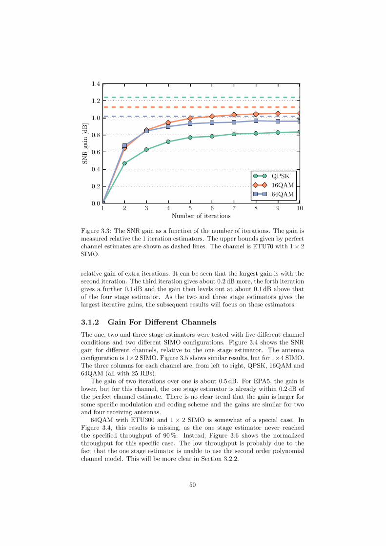
1 2 3 4 5 6 7 8 9 10Number of iterations

0.0

0.2

0.4

0.6

0.8

1.0

1.2

1.4S

NR

gain

[dB

]

QPSK

16QAM

64QAM

Figure 3.3: The SNR gain as a function of the number of iterations. The gain ismeasured relative the 1 iteration estimators. The upper bounds given by perfectchannel estimates are shown as dashed lines. The channel is ETU70 with 1× 2SIMO.

relative gain of extra iterations. It can be seen that the largest gain is with thesecond iteration. The third iteration gives about 0.2 dB more, the forth iterationgives a further 0.1 dB and the gain then levels out at about 0.1 dB above thatof the four stage estimator. As the two and three stage estimators gives thelargest iterative gains, the subsequent results will focus on these estimators.

3.1.2 Gain For Different Channels

The one, two and three stage estimators were tested with five different channelconditions and two different SIMO configurations. Figure 3.4 shows the SNRgain for different channels, relative to the one stage estimator. The antennaconfiguration is 1×2 SIMO. Figure 3.5 shows similar results, but for 1×4 SIMO.The three columns for each channel are, from left to right, QPSK, 16QAM and64QAM (all with 25 RBs).

The gain of two iterations over one is about 0.5 dB. For EPA5, the gain islower, but for this channel, the one stage estimator is already within 0.2 dB ofthe perfect channel estimate. There is no clear trend that the gain is larger forsome specific modulation and coding scheme and the gains are similar for twoand four receiving antennas.

64QAM with ETU300 and 1 × 2 SIMO is somewhat of a special case. InFigure 3.4, this results is missing, as the one stage estimator never reachedthe specified throughput of 90 %. Instead, Figure 3.6 shows the normalizedthroughput for this specific case. The low throughput is probably due to thefact that the one stage estimator is unable to use the second order polynomialchannel model. This will be more clear in Section 3.2.2.

50

EPA5 EVA70 ETU5 ETU70 ETU3000.0

0.5

1.0

1.5

2.0

SN

Rga

in[d

B]

Perfect

3it

2it

Figure 3.4: The SNR gain for different channels. The gain is measured relativethe one stage estimator. The three columns for each channel correspond toQPSK, 16QAM and 64QAM. The antenna configuration is 1 × 2 SIMO. The64QAM results are missing for ETU300.

EPA5 EVA70 ETU5 ETU70 ETU3000.0

0.5

1.0

1.5

2.0

2.5

3.0

3.5

SN

Rga

in[d

B]

Perfect

3it

2it

Figure 3.5: This figure shows the same kind of data as Figure 3.4, but for 1× 4SIMO.

51

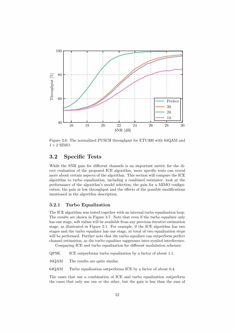
16 18 20 22 24 26 28 30

SNR [dB]

40

60

80

100T

hro

ugh

pu

t[%

]

Perfect

3it

2it

1it

Figure 3.6: The normalized PUSCH throughput for ETU300 with 64QAM and1× 2 SIMO.

3.2 Specific Tests

While the SNR gain for different channels is an important metric for the di-rect evaluation of the proposed ICE algorithm, more specific tests can revealmore about certain aspects of the algorithm. This section will compare the ICEalgorithm to turbo equalization, including a combined estimator, look at theperformance of the algorithm’s model selection, the gain for a MIMO configu-ration, the gain at low throughput and the effects of the possible modificationsmentioned in the algorithm description.

3.2.1 Turbo Equalization

The ICE algorithm was tested together with an internal turbo equalization loop.The results are shown in Figure 3.7. Note that even if the turbo equalizer onlyhas one stage, soft values will be available from any previous iterative estimationstage, as illustrated in Figure 2.1. For example, if the ICE algorithm has twostages and the turbo equalizer has one stage, at total of two equalization stepswill be performed. Further note that the turbo equalizer can outperform perfectchannel estimation, as the turbo equalizer suppresses inter-symbol interference.

Comparing ICE and turbo equalization for different modulation schemes:

QPSK ICE outperforms turbo equalization by a factor of about 1.1.

16QAM The results are quite similar.

64QAM Turbo equalization outperforms ICE by a factor of about 0.4.

The cases that use a combination of ICE and turbo equalization outperformthe cases that only use one or the other, but the gain is less than the sum of

52

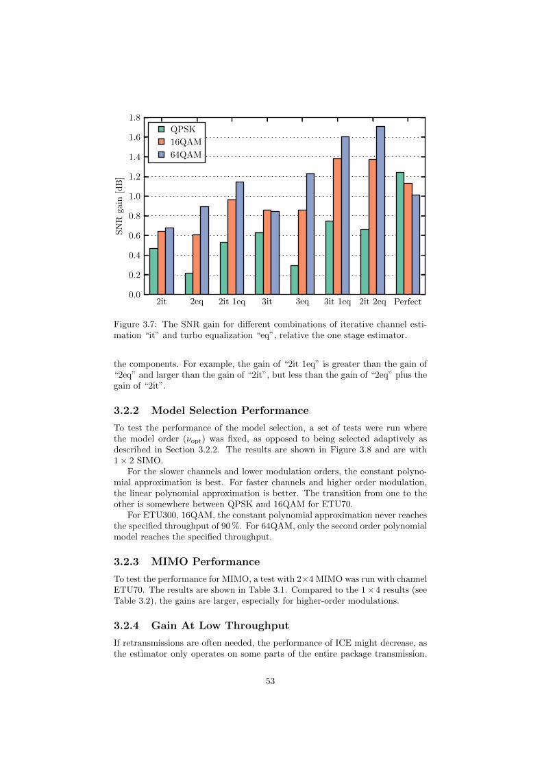
2it 2eq 2it 1eq 3it 3eq 3it 1eq 2it 2eq Perfect0.0

0.2

0.4

0.6

0.8

1.0

1.2

1.4

1.6

1.8S

NR

gain

[dB

]QPSK

16QAM

64QAM

Figure 3.7: The SNR gain for different combinations of iterative channel esti-mation “it” and turbo equalization “eq”, relative the one stage estimator.

the components. For example, the gain of “2it 1eq” is greater than the gain of“2eq” and larger than the gain of “2it”, but less than the gain of “2eq” plus thegain of “2it”.

3.2.2 Model Selection Performance

To test the performance of the model selection, a set of tests were run wherethe model order (νopt) was fixed, as opposed to being selected adaptively asdescribed in Section 3.2.2. The results are shown in Figure 3.8 and are with1× 2 SIMO.

For the slower channels and lower modulation orders, the constant polyno-mial approximation is best. For faster channels and higher order modulation,the linear polynomial approximation is better. The transition from one to theother is somewhere between QPSK and 16QAM for ETU70.

For ETU300, 16QAM, the constant polynomial approximation never reachesthe specified throughput of 90 %. For 64QAM, only the second order polynomialmodel reaches the specified throughput.

3.2.3 MIMO Performance

To test the performance for MIMO, a test with 2×4 MIMO was run with channelETU70. The results are shown in Table 3.1. Compared to the 1× 4 results (seeTable 3.2), the gains are larger, especially for higher-order modulations.

3.2.4 Gain At Low Throughput

If retransmissions are often needed, the performance of ICE might decrease, asthe estimator only operates on some parts of the entire package transmission.

53

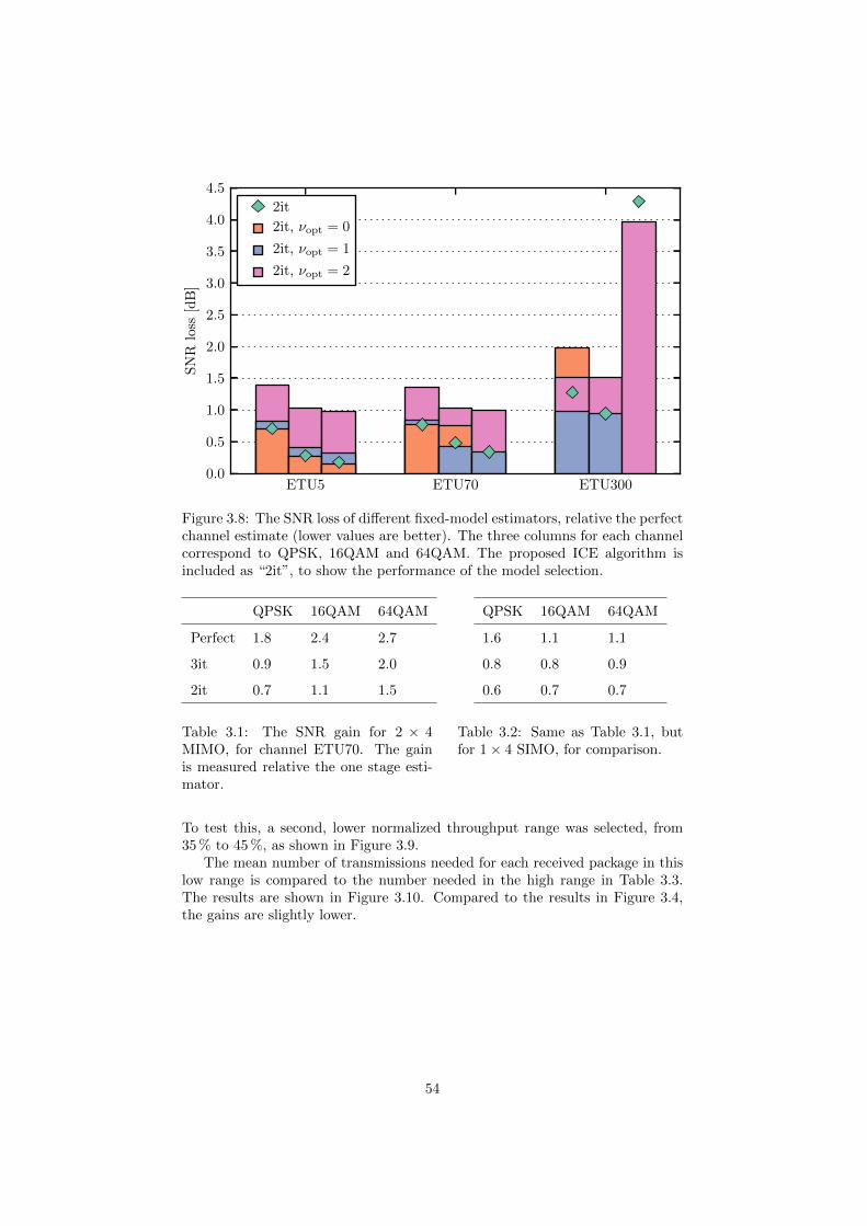
ETU5 ETU70 ETU3000.0

0.5

1.0

1.5

2.0

2.5

3.0

3.5

4.0

4.5S

NR

loss

[dB

]2it

2it, νopt = 0

2it, νopt = 1

2it, νopt = 2

Figure 3.8: The SNR loss of different fixed-model estimators, relative the perfectchannel estimate (lower values are better). The three columns for each channelcorrespond to QPSK, 16QAM and 64QAM. The proposed ICE algorithm isincluded as “2it”, to show the performance of the model selection.

QPSK 16QAM 64QAM

Perfect 1.8 2.4 2.7

3it 0.9 1.5 2.0

2it 0.7 1.1 1.5

Table 3.1: The SNR gain for 2 × 4MIMO, for channel ETU70. The gainis measured relative the one stage esti-mator.

QPSK 16QAM 64QAM

1.6 1.1 1.1

0.8 0.8 0.9

0.6 0.7 0.7

Table 3.2: Same as Table 3.1, butfor 1× 4 SIMO, for comparison.

To test this, a second, lower normalized throughput range was selected, from35 % to 45 %, as shown in Figure 3.9.

The mean number of transmissions needed for each received package in thislow range is compared to the number needed in the high range in Table 3.3.The results are shown in Figure 3.10. Compared to the results in Figure 3.4,the gains are slightly lower.

54

−10 −5 0 5 10 15 20 25 30

SNR [dB]

0

20

40

60

80

100T

hro

ugh

pu

t[%

]

Perfect

2it

1it

Figure 3.9: The gray-shaded region was used to measure the SNR gain in caseswhere the throughput is low.

Throughput Transmissions per package

High 1.1 to 1.4

Low 2.2 to 2.9

Table 3.3: Number of transmissions per package.

3.2.5 Effect Of Modifications

In the algorithm description, some possible modifications were mentioned. Thesemodifications were applied to the the stage estimator and tested for ETU70 with1× 2 SIMO. The results are summarized here.

• Soft and hard bit feedback were indistinguishable from each other.

• The assumption σxx = σx was indistinguishable from an estimated σxx.

• The assumption σ2x = 1 resulted in an SNR loss of a small fraction of a

dB at very low throughput, compared to an estimated σ2x.

55

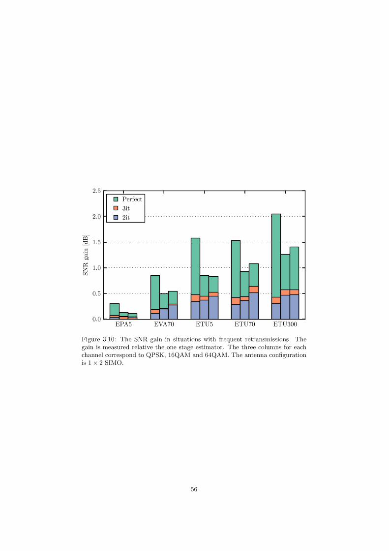
EPA5 EVA70 ETU5 ETU70 ETU3000.0

0.5

1.0

1.5

2.0

2.5

SN

Rga

in[d

B]

Perfect

3it

2it

Figure 3.10: The SNR gain in situations with frequent retransmissions. Thegain is measured relative the one stage estimator. The three columns for eachchannel correspond to QPSK, 16QAM and 64QAM. The antenna configurationis 1× 2 SIMO.

56

Chapter 4

Discussion

This chapter will discuss the simulation results, the complexity and implemen-tation issues of the proposed algorithm, possible future works and finally sum-marize the thesis.

4.1 Results

This section will discuss some of the results from the simulations.

4.1.1 Gain For Different Channels

The results indicates gain of about 0.5 dB to 0.8 dB for 2 to 4 stages of ICE, quitesimilar to the results reported by [44] for MMSE-based ICE in LTE downlink.If the SNR-gap to the perfect channel estimate is small, the ICE algorithm canprovide near-ideal channel estimation. Using a two or three stage estimator ismost attractive from a cost/benefit perspective, as any further iterations onlyprovides marginal gains.

A special case is very fast varying channels at high SNR. In these conditions,the throughput is limited not by receiver noise, but by the quality of the channelestimate. By using the data symbols as extra pilot symbols, the fast variationsof the channel can be better tracked, which leads to increased throughput.

4.1.2 Turbo Equalization

Iterative channel estimation seems to provide larger gain than turbo equalizationfor QPSK, while the opposite is true for 64QAM. For 16QAM, the results aresimilar. In theory, a combination of ICE and turbo equalization should providelarger gains then the gain of the separate parts. The rational is that the iterativechannel estimator improves the channel estimate used by the equalizer and theequalizer improves the decoded bits used by the channel estimator. But inpractice, the gain of the combined processing was less then the sum of the gainsof the parts.

57

4.1.3 MIMO Performance

The MIMO results showed some unexpected differences compared to the SIMOresults:

• The gain overall is higher.

• The gains are markedly higher for the higher-order modulation schemes,while for SIMO, all modulation schemes have a similar gain.

• The SNR-gap to the perfect channel estimate is smaller for the lower ordermodulation, while the opposite is true for SIMO.

The reasons for these differences are unclear. Perhaps the simple MRC + MMSEstructure used for antenna combining and equalization is more sensitive to chan-nel estimation errors for higher order modulations.

4.1.4 Modifications

It was unexpected that soft and hard bit feedback produced identical results,as [44] reported better performance for soft bits. They however looked at LTEdownlink, which does not use DFT-spreading, which may explain the difference.The DFT-spreading spreads errors introduced by hard bits over the entire sub-carrier range. This combined with the averaging across OFDM symbols mayeffectively suppress the errors.

The results for the variance and covariance of the regenerated symbols indi-cates that the regenerated symbols typically are well correlated with the actualsymbols (σxx = σx), but that the loss of energy (σ2

x < 1) should be accountedfor.

4.2 Complexity

The asymptotic complexity of the ICE algorithm is O (n log2 n), in the numberof subcarriers, as it is bounded by the complexity of the FFT operations, allother stages have linear complexity.

Finding the soft time-domain symbols only requires a few operations persymbol, and is an embarrassingly parallel problem. The complexity of the sym-bols regeneration is thus bounded by the complexity of the DFT-spreading.

Computing point-wise channel estimates is linear in the number of OFDMsymbols and subcarriers. Further, each subcarrier can be processed indepen-dently, if for example a single-instruction, multiple-data (SIMD) architecture isavailable.

The DCT operations required for model selection and channel filtering arecomplication factors from an implementation standpoint. One DCT operationfor model selection and one IDCT for channel filtering is always needed. Butas much as four DCTs plus three IDCTs might be needed (one DCT for modelselection and three DCTs and IDCTs for channel filtering when νopt = 2). Thismakes the latency hard to predict. Further, if the architecture can executeDCTs in parallel, the designer must decide if all DCTs that might be neededshould be executed simultaneously, discarding unused results, or if executionshould be held off until the model has been selected. The first method reduces

58

latency, but increases base station power usage and processor load. A thirdoption is to use a predictor to guess what DCTs will be needed.

Once the channel coefficients have been filtered, regenerating the channel islinear in the number of subcarriers and OFDM symbols.

4.3 Further Work

These are some suggestions for topics that could be further explored.

4.3.1 Reduce Complexity of Iterations

ICE means that all receiver stages inside the iterative estimation loop must berun multiple times. Any simplification of the internal stages will thus have alarge impact on the complexity of the whole receiver chain. The most obviouspossibility for simplifications is the turbo decoder, which forms the innermostloop. For this thesis, the decoder does not retain extrinsic information betweeniterative estimation stages. It is possible that retaining that information couldreduce the number of iterations needed, without impacting the decoding per-formance.

4.3.2 Improved Heuristics

The proposed algorithm uses heuristics for channel length estimation and modelselection. While these heuristics do not directly relate to ICE, good heuristicscould improve the performance in absolute terms.

One clear possibility for improvements is to make the model selection awareof the channel length. If the channel is short, it may be appropriate to selecta higher order approximation even at high noise levels, as the channel filteringwill provide higher noise suppression for shorter channels.

The heuristic criteria include some free parameters, which tune the behaviorof the heuristics. To select these parameters, numerical optimization could beused. This requires a goal function which is to be optimized, for example theweighted-average throughput for different channel models.

4.3.3 Implementation On Hardware

To accurately gauge the computational complexity and performance of the pro-posed algorithm, it should be implemented on actual base station hardware.

4.4 Conclusions

An iterative channel estimation algorithm has been proposed. The algorithmoperates on LTE subframes and uses soft symbol feedback, a polynomial modelacross OFDM symbols and DCT-based filtering across subcarriers. The algo-rithm has an asymptotic complexity of O (n log2 n), is suited for parallel imple-mentations and does not require detailed channel knowledge. With two estima-tion stages, a gain of about 0.5 dB can be achieved in many cases, with a further0.2 dB extra gain if three stages are used.

59

On average, turbo equalization provides similar performance to ICE. Fur-ther, by using turbo equalization, the throughput can surpass what is possibleeven with ideal channel estimation. Turbo equalization also has lower complex-ity than ICE. Thus, turbo equalization is a more attractive receiver structurethan ICE, if only one of the two methods can be used.

60

Bibliography

[1] E. Dahlman, S. Parkvall, and J. Skold, 4G: LTE/LTE-Advanced for MobileBroadband: LTE/LTE-Advanced for Mobile Broadband. Elsevier Science,2011.

[2] S. Ahmadi, LTE-Advanced: A Practical Systems Approach to Understand-ing 3GPP LTE Releases 10 and 11 Radio Access Technologies. ElsevierScience, 2013.

[3] 3GPP, “About 3GPP.” http://www.3gpp.org/about-3gpp (visited on2014-03-22).

[4] International Telecommunication Union, “International Mobile Telecom-munications 2000 (IMT-2000).” ITU-R Recommendation M.687-2, Febru-ary 1997.

[5] 3GPP, “Technical Specification Group Radio Access Network; Require-ments for Evolved UTRA (E-UTRA) and Evolved UTRAN (E-UTRAN)(Release 8),” TR 25.913, 3rd Generation Partnership Project (3GPP), Dec.2008.

[6] TeliaSonera, “TeliaSonera first in the world with 4G services.”http://www.teliasonera.com/en/newsroom/press-releases/2009/

12/teliasonera-first-in-the-world-with-4g-services/ (visited on2014-03-22), December 2009.

[7] S. Parkvall, E. Dahlman, A. Furuskar, Y. Jading, M. Olsson, S. Wanstedt,and K. Zangi, “LTE-Advanced - evolving LTE towards IMT-Advanced,” inVehicular Technology Conference, 2008. VTC 2008-Fall. IEEE 68th, pp. 1–5, Sept 2008.

[8] C. E. Shannon, “A mathematical theory of communication,” Bell systemtechnical journal, vol. 27, 1948.

[9] S. Haykin, Communication systems. Wiley, 2001.

[10] 3GPP, “Evolved Universal Terrestrial Radio Access (E-UTRA); Physicalchannels and modulation,” TS 36.211, 3rd Generation Partnership Project(3GPP), June 2009.

[11] A. Viterbi and J. Omura, Principles of digital communication and coding.McGraw-Hill series in electrical engineering, McGraw-Hill, 1979.

61

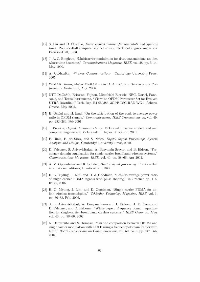
[12] S. Lin and D. Costello, Error control coding: fundamentals and applica-tions. Prentice-Hall computer applications in electrical engineering series,Prentice-Hall, 1983.

[13] J. A. C. Bingham, “Multicarrier modulation for data transmission: an ideawhose time has come,” Communications Magazine, IEEE, vol. 28, pp. 5–14,May 1990.

[14] A. Goldsmith, Wireless Communications. Cambridge University Press,2005.

[15] WiMAX Forum, Mobile WiMAX – Part I: A Technical Overview and Per-formance Evaluation, Aug. 2006.

[16] NTT DoCoMo, Ericsson, Fujitsu, Mitsubishi Electric, NEC, Nortel, Pana-sonic, and Texas Instruments, “Views on OFDM Parameter Set for EvolvedUTRA Downlink,” Tech. Rep. R1-050386, 3GPP TSG-RAN WG 1, Athens,Greece, May 2005.

[17] H. Ochiai and H. Imai, “On the distribution of the peak-to-average powerratio in OFDM signals,” Communications, IEEE Transactions on, vol. 49,pp. 282–289, Feb 2001.

[18] J. Proakis, Digital Communications. McGraw-Hill series in electrical andcomputer engineering, McGraw-Hill Higher Education, 2001.

[19] P. Diniz, E. da Silva, and S. Netto, Digital Signal Processing: SystemAnalysis and Design. Cambridge University Press, 2010.

[20] D. Falconer, S. Ariyavisitakul, A. Benyamin-Seeyar, and B. Eidson, “Fre-quency domain equalization for single-carrier broadband wireless systems,”Communications Magazine, IEEE, vol. 40, pp. 58–66, Apr 2002.

[21] A. V. Oppenheim and R. Schafer, Digital signal processing. Prentice-Hallinternational editions, Prentice-Hall, 1975.

[22] H. G. Myung, J. Lim, and D. J. Goodman, “Peak-to-average power ratioof single carrier FDMA signals with pulse shaping,” in PIMRC, pp. 1–5,IEEE, 2006.

[23] H. G. Myung, J. Lim, and D. Goodman, “Single carrier FDMA for up-link wireless transmission,” Vehicular Technology Magazine, IEEE, vol. 1,pp. 30–38, Feb. 2006.

[24] S. L. Ariyavisitakul, A. Benyamin-seeyar, B. Eidson, B. E. Conexant,D. Falconer, and D. Falconer, “White paper: Frequency domain equaliza-tion for single-carrier broadband wireless systems,” IEEE Commun. Mag,vol. 40, pp. 58–66, 2002.

[25] N. Benvenuto and S. Tomasin, “On the comparison between OFDM andsingle carrier modulation with a DFE using a frequency-domain feedforwardfilter,” IEEE Transactions on Communications, vol. 50, no. 6, pp. 947–955,2002.

62

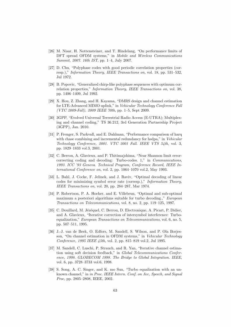
[26] M. Nisar, H. Nottensteiner, and T. Hindelang, “On performance limits ofDFT spread OFDM systems,” in Mobile and Wireless CommunicationsSummit, 2007. 16th IST, pp. 1–4, July 2007.

[27] D. Chu, “Polyphase codes with good periodic correlation properties (cor-resp.),” Information Theory, IEEE Transactions on, vol. 18, pp. 531–532,Jul 1972.

[28] B. Popovic, “Generalized chirp-like polyphase sequences with optimum cor-relation properties,” Information Theory, IEEE Transactions on, vol. 38,pp. 1406–1409, Jul 1992.

[29] X. Hou, Z. Zhang, and H. Kayama, “DMRS design and channel estimationfor LTE-Advanced MIMO uplink,” in Vehicular Technology Conference Fall(VTC 2009-Fall), 2009 IEEE 70th, pp. 1–5, Sept 2009.

[30] 3GPP, “Evolved Universal Terrestrial Radio Access (E-UTRA); Multiplex-ing and channel coding,” TS 36.212, 3rd Generation Partnership Project(3GPP), Jan. 2010.

[31] P. Frenger, S. Parkvall, and E. Dahlman, “Performance comparison of harqwith chase combining and incremental redundancy for hsdpa,” in VehicularTechnology Conference, 2001. VTC 2001 Fall. IEEE VTS 54th, vol. 3,pp. 1829–1833 vol.3, 2001.

[32] C. Berrou, A. Glavieux, and P. Thitimajshima, “Near Shannon limit error-correcting coding and decoding: Turbo-codes. 1,” in Communications,1993. ICC ’93 Geneva. Technical Program, Conference Record, IEEE In-ternational Conference on, vol. 2, pp. 1064–1070 vol.2, May 1993.

[33] L. Bahl, J. Cocke, F. Jelinek, and J. Raviv, “Optimal decoding of linearcodes for minimizing symbol error rate (corresp.),” Information Theory,IEEE Transactions on, vol. 20, pp. 284–287, Mar 1974.

[34] P. Robertson, P. A. Hoeher, and E. Villebrun, “Optimal and sub-optimalmaximum a posteriori algorithms suitable for turbo decoding.,” EuropeanTransactions on Telecommunications, vol. 8, no. 2, pp. 119–125, 1997.

[35] C. Douillard, M. Jezequel, C. Berrou, D. Electronique, A. Picart, P. Didier,and A. Glavieux, “Iterative correction of intersymbol interference: Turbo-equalization,” European Transactions on Telecommunications, vol. 6, no. 5,pp. 507–511, 1995.

[36] J.-J. van de Beek, O. Edfors, M. Sandell, S. Wilson, and P. Ola Borjes-son, “On channel estimation in OFDM systems,” in Vehicular TechnologyConference, 1995 IEEE 45th, vol. 2, pp. 815–819 vol.2, Jul 1995.

[37] M. Sandell, C. Luschi, P. Strauch, and R. Yan, “Iterative channel estima-tion using soft decision feedback,” in Global Telecommunications Confer-ence, 1998. GLOBECOM 1998. The Bridge to Global Integration. IEEE,vol. 6, pp. 3728–3733 vol.6, 1998.

[38] S. Song, A. C. Singer, and K. mo Sun, “Turbo equalization with an un-known channel,” in in Proc. IEEE Intern. Conf. on Acc, Speech, and SignalProc, pp. 2805–2808, IEEE, 2002.

63

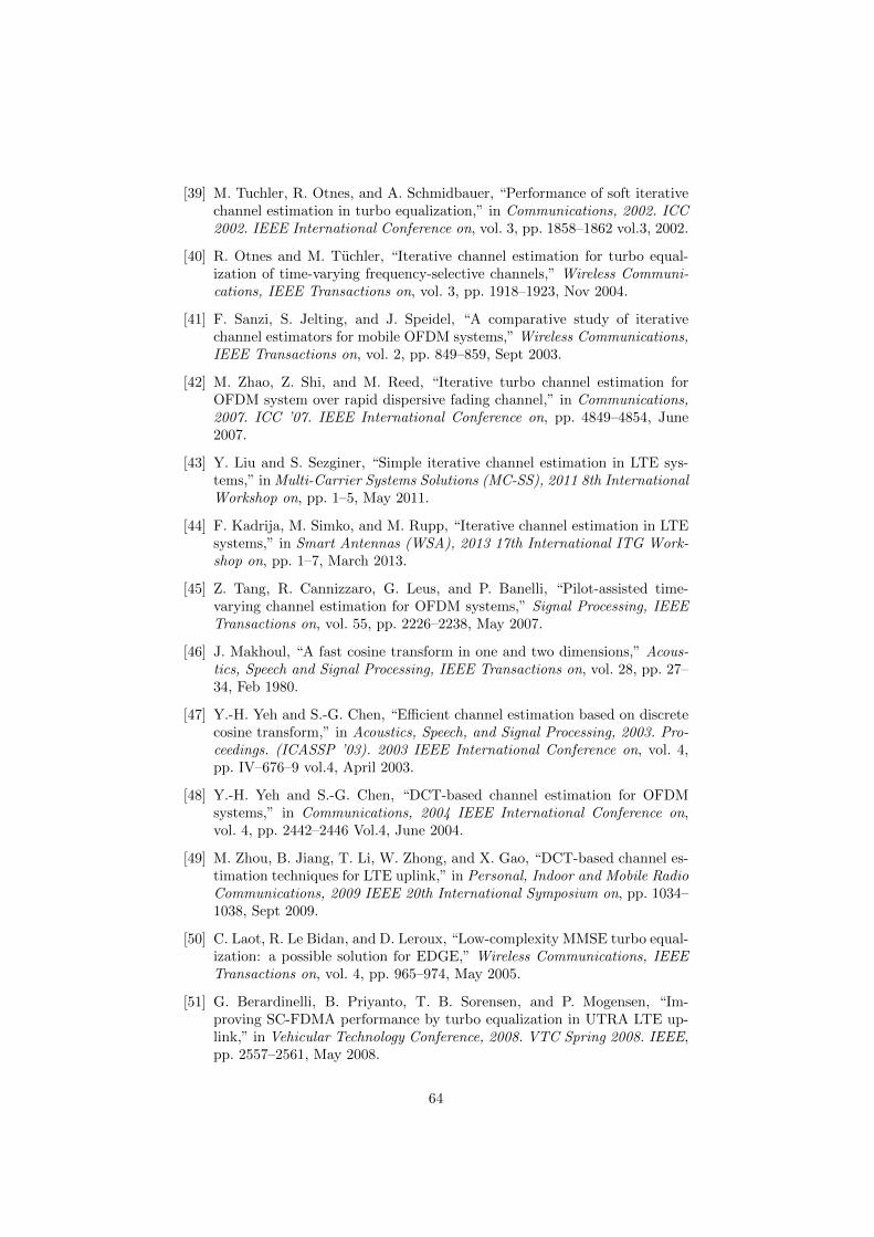
[39] M. Tuchler, R. Otnes, and A. Schmidbauer, “Performance of soft iterativechannel estimation in turbo equalization,” in Communications, 2002. ICC2002. IEEE International Conference on, vol. 3, pp. 1858–1862 vol.3, 2002.

[40] R. Otnes and M. Tuchler, “Iterative channel estimation for turbo equal-ization of time-varying frequency-selective channels,” Wireless Communi-cations, IEEE Transactions on, vol. 3, pp. 1918–1923, Nov 2004.

[41] F. Sanzi, S. Jelting, and J. Speidel, “A comparative study of iterativechannel estimators for mobile OFDM systems,” Wireless Communications,IEEE Transactions on, vol. 2, pp. 849–859, Sept 2003.

[42] M. Zhao, Z. Shi, and M. Reed, “Iterative turbo channel estimation forOFDM system over rapid dispersive fading channel,” in Communications,2007. ICC ’07. IEEE International Conference on, pp. 4849–4854, June2007.

[43] Y. Liu and S. Sezginer, “Simple iterative channel estimation in LTE sys-tems,” in Multi-Carrier Systems Solutions (MC-SS), 2011 8th InternationalWorkshop on, pp. 1–5, May 2011.

[44] F. Kadrija, M. Simko, and M. Rupp, “Iterative channel estimation in LTEsystems,” in Smart Antennas (WSA), 2013 17th International ITG Work-shop on, pp. 1–7, March 2013.

[45] Z. Tang, R. Cannizzaro, G. Leus, and P. Banelli, “Pilot-assisted time-varying channel estimation for OFDM systems,” Signal Processing, IEEETransactions on, vol. 55, pp. 2226–2238, May 2007.

[46] J. Makhoul, “A fast cosine transform in one and two dimensions,” Acous-tics, Speech and Signal Processing, IEEE Transactions on, vol. 28, pp. 27–34, Feb 1980.

[47] Y.-H. Yeh and S.-G. Chen, “Efficient channel estimation based on discretecosine transform,” in Acoustics, Speech, and Signal Processing, 2003. Pro-ceedings. (ICASSP ’03). 2003 IEEE International Conference on, vol. 4,pp. IV–676–9 vol.4, April 2003.

[48] Y.-H. Yeh and S.-G. Chen, “DCT-based channel estimation for OFDMsystems,” in Communications, 2004 IEEE International Conference on,vol. 4, pp. 2442–2446 Vol.4, June 2004.

[49] M. Zhou, B. Jiang, T. Li, W. Zhong, and X. Gao, “DCT-based channel es-timation techniques for LTE uplink,” in Personal, Indoor and Mobile RadioCommunications, 2009 IEEE 20th International Symposium on, pp. 1034–1038, Sept 2009.

[50] C. Laot, R. Le Bidan, and D. Leroux, “Low-complexity MMSE turbo equal-ization: a possible solution for EDGE,” Wireless Communications, IEEETransactions on, vol. 4, pp. 965–974, May 2005.

[51] G. Berardinelli, B. Priyanto, T. B. Sorensen, and P. Mogensen, “Im-proving SC-FDMA performance by turbo equalization in UTRA LTE up-link,” in Vehicular Technology Conference, 2008. VTC Spring 2008. IEEE,pp. 2557–2561, May 2008.

64

[52] J. Cheng, “Fast soft value computation methods for gray-mapped qam,”Jan. 1 2008. US Patent 7,315,578.

[53] 3GPP, “Evolved Universal Terrestrial Radio Access (E-UTRA); UserEquipment (UE) radio transmission and reception,” TS 36.101, 3rd Gen-eration Partnership Project (3GPP), Mar. 2014.

[54] W. C. Jakes and D. C. Cox, eds., Microwave Mobile Communications.Wiley-IEEE Press, 1994.

65