pltmg - sandia national laboratories
TRANSCRIPT

PLTMG:A Software Packagefor Solving Elliptic PartialDifferential Equations
Users’ Guide 13.0
Randolph E. Bank
Department of MathematicsUniversity of California at San DiegoLa Jolla, California 92093-0112
September, 2018

ii PLTMG USERS’ GUIDE 13.0
Copyright (c) 2018, by the author.
This work was supported by the National Science Foundationunder grants DMS-1318480, DMS-1345103, and MRI-0821816.
This software is made available for research and instructional use only. You may copyand use this software without charge for these non-commercial purposes, provided thatthe copyright notice and associated text is reproduced on all copies. For all other uses(including distribution of modified versions), please contact the author. This softwareis provided “as is”, without any expressed or implied warranty. In particular, theauthor does not make any representation or warranty of any kind concerning thefitness of this software for any particular purpose.


iv PLTMG USERS’ GUIDE 13.0

Contents
Preface ix
1 Introduction 11.1 Problem Specification. . . . . . . . . . . . . . . . . . . . . . . . 1
1.1.1 Approximation Spaces. . . . . . . . . . . . . . . . . 21.1.2 Elliptic Boundary Value Problem. . . . . . . . . . . 31.1.3 Obstacle Problem. . . . . . . . . . . . . . . . . . . . 31.1.4 Continuation Problem. . . . . . . . . . . . . . . . . 41.1.5 Parameter Identification Problem. . . . . . . . . . . 41.1.6 Optimal Control Problem. . . . . . . . . . . . . . . . 5
1.2 Main Subroutines . . . . . . . . . . . . . . . . . . . . . . . . . . 61.3 Installation. . . . . . . . . . . . . . . . . . . . . . . . . . . . . . 7
2 Data Structures 92.1 Overview. . . . . . . . . . . . . . . . . . . . . . . . . . . . . . . 92.2 Edge Definitions . . . . . . . . . . . . . . . . . . . . . . . . . . . 10
2.2.1 Curved Edges – Circular Arcs . . . . . . . . . . . . 102.2.2 Curved Edges – Parametric . . . . . . . . . . . . . . 11
2.3 The Triangulation. . . . . . . . . . . . . . . . . . . . . . . . . . 132.4 The Skeleton. . . . . . . . . . . . . . . . . . . . . . . . . . . . . 142.5 Finite Element Data Structures. . . . . . . . . . . . . . . . . . . 192.6 Parallel Processing Data Structure. . . . . . . . . . . . . . . . . 212.7 Parameter Arrays. . . . . . . . . . . . . . . . . . . . . . . . . . . 222.8 Coefficient Functions. . . . . . . . . . . . . . . . . . . . . . . . . 282.9 Sparse Matrix Storage. . . . . . . . . . . . . . . . . . . . . . . . 33
3 Mesh Generation 373.1 Overview. . . . . . . . . . . . . . . . . . . . . . . . . . . . . . . 373.2 Creating a Triangulation from a Skeleton. . . . . . . . . . . . . 383.3 A Posteriori Error Estimates. . . . . . . . . . . . . . . . . . . . 413.4 Adaptive Mesh Refinement and Unrefinement. . . . . . . . . . . 43
3.4.1 Procedure Refine . . . . . . . . . . . . . . . . . . . 443.4.2 Procedure Unrefine . . . . . . . . . . . . . . . . . . 453.4.3 h Refinement . . . . . . . . . . . . . . . . . . . . . . 46
v

vi Contents
3.4.4 h Unrefinement . . . . . . . . . . . . . . . . . . . . . 473.4.5 p Refinement . . . . . . . . . . . . . . . . . . . . . . 483.4.6 p Unrefinement . . . . . . . . . . . . . . . . . . . . . 48
3.5 Adaptive Mesh Smoothing. . . . . . . . . . . . . . . . . . . . . . 483.6 Uniform Refinement. . . . . . . . . . . . . . . . . . . . . . . . . 49
3.6.1 h Uniform Refinement . . . . . . . . . . . . . . . . . 503.6.2 p Uniform Refinement . . . . . . . . . . . . . . . . . 50
3.7 An Example . . . . . . . . . . . . . . . . . . . . . . . . . . . . . 513.8 Parallel Adaptive Methods. . . . . . . . . . . . . . . . . . . . . . 51
3.8.1 Mesh Partitioning. . . . . . . . . . . . . . . . . . . . 553.8.2 Reconciling the Mesh. . . . . . . . . . . . . . . . . . 57
4 Equation Solution 594.1 Overview. . . . . . . . . . . . . . . . . . . . . . . . . . . . . . . 594.2 Elliptic Boundary Value Problems. . . . . . . . . . . . . . . . . 604.3 Linear Solvers. . . . . . . . . . . . . . . . . . . . . . . . . . . . . 624.4 Domain Decomposition Solver . . . . . . . . . . . . . . . . . . . 654.5 Obstacle Problems. . . . . . . . . . . . . . . . . . . . . . . . . . 664.6 Continuation Problems. . . . . . . . . . . . . . . . . . . . . . . . 684.7 Parameter Identification Problems. . . . . . . . . . . . . . . . . 744.8 Optimal Control Problems. . . . . . . . . . . . . . . . . . . . . . 78
5 Graphics 835.1 Overview. . . . . . . . . . . . . . . . . . . . . . . . . . . . . . . 835.2 Subroutine TRIPLT. . . . . . . . . . . . . . . . . . . . . . . . . 84
5.2.1 Surface Plots. . . . . . . . . . . . . . . . . . . . . . . 875.2.2 Vector Plots. . . . . . . . . . . . . . . . . . . . . . . 885.2.3 Parameters RMAG, CENX, and CENY. . . . . . . . 885.2.4 Parameters ISCALE, LINES, NUMBRS, and MPIRGN. 895.2.5 Parameters ICRSN and ITRGT. . . . . . . . . . . . 895.2.6 Some Algorithmic Details. . . . . . . . . . . . . . . . 91
5.3 Subroutine INPLT. . . . . . . . . . . . . . . . . . . . . . . . . . 915.3.1 Triangle Plots. . . . . . . . . . . . . . . . . . . . . . 925.3.2 Skeleton Plots. . . . . . . . . . . . . . . . . . . . . . 93
5.4 Subroutine GPHPLT. . . . . . . . . . . . . . . . . . . . . . . . . 945.4.1 Iteration Information. . . . . . . . . . . . . . . . . . 945.4.2 Timing Statistics. . . . . . . . . . . . . . . . . . . . 975.4.3 Continuation Path. . . . . . . . . . . . . . . . . . . . 985.4.4 Parallel Statistics . . . . . . . . . . . . . . . . . . . 985.4.5 Error Estimates. . . . . . . . . . . . . . . . . . . . . 985.4.6 Displaying Data Arrays. . . . . . . . . . . . . . . . . 99
6 Test Driver 1016.1 Overview. . . . . . . . . . . . . . . . . . . . . . . . . . . . . . . 1016.2 Terminal Mode. . . . . . . . . . . . . . . . . . . . . . . . . . . . 1026.3 Web Browser Mode. . . . . . . . . . . . . . . . . . . . . . . . . . 104

Contents vii
6.4 Batch Mode. . . . . . . . . . . . . . . . . . . . . . . . . . . . . . 1096.5 Parallel Processing . . . . . . . . . . . . . . . . . . . . . . . . . 1096.6 Command Line Parameters . . . . . . . . . . . . . . . . . . . . . 1106.7 Array Dimensions and Initialization. . . . . . . . . . . . . . . . 1116.8 Reading and Writing Files. . . . . . . . . . . . . . . . . . . . . . 1126.9 Journal Files. . . . . . . . . . . . . . . . . . . . . . . . . . . . . 1126.10 Subroutine USRCMD. . . . . . . . . . . . . . . . . . . . . . . . 1126.11 Subroutine GDATA. . . . . . . . . . . . . . . . . . . . . . . . . . 1146.12 Machine Dependent Routines. . . . . . . . . . . . . . . . . . . . 115
6.12.1 Arithmetic Specification. . . . . . . . . . . . . . . . 1156.12.2 Timing Routine. . . . . . . . . . . . . . . . . . . . . 1166.12.3 Command Line Interface . . . . . . . . . . . . . . . 1176.12.4 Graphics Interface. . . . . . . . . . . . . . . . . . . . 1176.12.5 MPI Interface . . . . . . . . . . . . . . . . . . . . . . 120
7 Test Problems 1217.1 Overview. . . . . . . . . . . . . . . . . . . . . . . . . . . . . . . 1217.2 Test Problem CIRCLE. . . . . . . . . . . . . . . . . . . . . . . . 1217.3 Test Problem SQUARE. . . . . . . . . . . . . . . . . . . . . . . 1227.4 Test Problem DOMAINS. . . . . . . . . . . . . . . . . . . . . . 1247.5 Test Problem NACA. . . . . . . . . . . . . . . . . . . . . . . . . 1247.6 Test Problem JCN. . . . . . . . . . . . . . . . . . . . . . . . . . 1267.7 Test Problem OB. . . . . . . . . . . . . . . . . . . . . . . . . . . 1277.8 Test Problem MNSURF. . . . . . . . . . . . . . . . . . . . . . . 1287.9 Test Problem BURGER. . . . . . . . . . . . . . . . . . . . . . . 1287.10 Test Problem BATTERY. . . . . . . . . . . . . . . . . . . . . . 1297.11 Test Problem CONTROL. . . . . . . . . . . . . . . . . . . . . . 1297.12 Test Problem IDENT. . . . . . . . . . . . . . . . . . . . . . . . 1307.13 Test Problem BOX. . . . . . . . . . . . . . . . . . . . . . . . . . 1317.14 Test Problem MESSAGE. . . . . . . . . . . . . . . . . . . . . . 1317.15 Test Problem USMAP. . . . . . . . . . . . . . . . . . . . . . . . 132
Bibliography 135
Index 141

viii Contents

Preface
Many people have made contributions to the development of this version of PLTMG;I am indebted to them all for their help. The original grid refinement algorithmsused in PLTMG were derived in 1976 as joint work with Todd Dupont of the Uni-versity of Chicago. The approximate Newton strategies incorporated in the presentversion of PLTMG represent joint work with Donald J. Rose. The gradient recov-ery and a posteriori error estimation procedures are joint work with Jinchao Xu ofPennsylvania State University and Bin Zheng of Pacific Northwest National Labora-tory. The algorithms used in the pseudo-arclength continuation procedures are jointwork with Tony Chan of the Hong Kong University of Science and Technology andHans Mittelmann of Arizona State University. The interior point algorithms usedin the optimization problems treated in this version are joint work with Philip Gillof University of California at San Diego. The adaptive mesh smoothing algorithmsare joint work with R. Kent Smith. The hp refinement algorithms and associateddata structures are joint work with Hieu Nguyen of the Universitat Politecnica DeCatalunya and Chris Deotte of the University of California at San Diego. The loadbalance algorithms for parallel computations are also joint work with Chris Deotte.The web browswer interface was developed and implemented by Chris Deotte. Theparallel adaptive paradigm is joint work with Michael Holst of the University ofCalifornia at San Diego. The parallel domain decomposition solver is joint workwith Shaoying Lu of the University of California at San Diego and Panayot Vas-silevski of Lawrence Livermore National Laboratory. The dual function used forparallel adaptive meshing is joint work with Jeffrey Ovall of Portland State Uni-versity. Many people made contributions to the test problems, reported bugs andsuggested improvements that have been incorporated in the current version.
This version of PLTMG was supported by the National Science Foundationthrough grants DMS-1318480 and DMS-1345013 (University of California at SanDiego). The UCSD Scicomp Beowulf cluster was built using funds provided by theNational Science Foundation through MRI-0821816.
University of California at San Diego Randolph E. BankSeptember, 2018
ix

x PLTMG USERS’ GUIDE 13.0

Chapter 1
Introduction
1.1 Problem Specification.Consider the elliptic boundary value problem
−∇ · a(x, y, u,∇u, λ) + f(x, y, u,∇u, λ) = 0 in Ω, (1.1)
with boundary conditions
u = g2(x, y, λ) on ∂Ω2,
a·n = g1(x, y, u, λ) on ∂Ω1, (1.2)
u, a·n continuous on ∂Ω0.
Here Ω is a bounded region in R2, n is the unit normal, a is the vector (a1, a2)t,a1, a2, f , g1, and g2 are scalar functions. ∂Ω0 is a portion of ∂Ω where periodicboundary conditions are applied. In some problems solved by PLTMG, the param-eter λ is not used, while in others λ ∈ Rk, k ≥ 1, is a vector of scalar parametersor λ ∈ H1(Ω), where H1(Ω) denotes the usual Sobolev space. Let
H1p = φ ∈ H1(Ω) |φ is continuous on ∂Ω0,H1g = φ ∈ H1
p |φ = g2 on ∂Ω2,H1e = φ ∈ H1
p |φ = 0 on ∂Ω2.
Then the weak form of (1.1)-(1.2) is: find u ∈ H1g such that
a(u, v) = 0 for all v ∈ H1e, (1.3)
where
a(u, v) =
∫Ω
a(u,∇u, λ) · ∇v + f(u,∇u, λ)v dx dy −∫∂Ω1
g1(u, λ)v ds. (1.4)
1

2 PLTMG USERS’ GUIDE 13.0
In some problems solved by PLTMG, a functional ρ(u, λ) plays an importantrole. Functionals we consider are of the form
ρ(u, λ) =
∫Ω
p1(x, y, u,∇u, λ) dx dy +
∫Γ
p2(x, y, u,∇u, λ) ds, (1.5)
where p1 and p2 are scalar functions. Here Γ = ∂Ω∪Γ0, where Γ0 consists of certaininternal curves specified by the user.
This version of the PLTMG package addresses five major problem classes.These are briefly described below.
1.1.1 Approximation Spaces.
PLTMG is based on a family of conforming C0 finite element spaces. Let T denotea triangulation of Ω and letM be the space of C0 piecewise polynomials associatedwith T . In this version of PLTMG, the degree of the polynomial can vary elementby element. The maximum degree allowed at present is p = 9, a condition imposedby the availability of suitable quadrature formulas.1 PLTMG represents such apiecewise polynomial using the standard Lagrange nodal basis; a function can thenbe specified by giving its values at the principle lattice points of the element, asillustrated in Figure 1.1 for the cases 1 ≤ p ≤ 3.
AAAAAAAAAA
y y
y
AAAAAAAAAA
y y
y
yy y
AAAAAAAAAA
y y
y
y y
y yy yy
Figure 1.1. Nodal degrees of freedom for the continuous piecewise linearelement, p = 1 (left), the continuous piecewise quadratic element, p = 2 (middle),and the continuous piecewise cubic element, p = 3 (right).
When two elements of different degrees share a common edge, the element oflower degree becomes a transition element. If such a element is of degree p, sharingan edge with an element of degree q > p, the element contains all polynomialsof degree p plus some additional polynomials of degree q, which allow the overallfinite element space to remain conforming. In particular, along the shared edge, thedegrees of freedom correspond to those of the higher degree element. Some examplesare given in Figure 1.2. Finally, PLTMG allows the use of isoparametric versions
1PLTMG uses quadrature formulas given in Zhang, Cui, and Liu [67].

1.1. Problem Specification. 3
AAAAAAAAAA
y y
y
y yy y
AAAAAAAAAA
y y y y
yy
y
y
yyyyy
Figure 1.2. Nodal degrees of freedom for the a quadratic transition ele-ment with a cubic edge (left), and a cubic transition element with one edge of degreefour and one edge of degree five (right).
of this family of Lagrange elements to address problems with curved boundaries orinterfaces.
1.1.2 Elliptic Boundary Value Problem.
For this problem, PLTMG solves a discrete analog of (1.3). The parameter λ doesnot play a role in this problem. Let I : H1(Ω) → M denote continuous piecewisepolynomial interpolation operator that interpolates at the degrees of freedom of T .Then
Mp = φ ∈M|φ is continuous on ∂Ω0,Mg = φ ∈Mp |φ = I(g2) on ∂Ω2,Me = φ ∈Mp |φ = 0 on ∂Ω2.
The discrete equations solved by PLTMG are formulated as follows: find uh ∈Md
such thata(uh, v) = 0 for all v ∈Me. (1.6)
1.1.3 Obstacle Problem.
The second class of problems addressed by PLTMG are the subset of variationalinequalities known as obstacle problems. Let
K = φ ∈ H1g |u ≤ φ ≤ u.
The obstacle problem is formulated as
minu∈K
ρ(u) (1.7)
where ρ is a functional of the form (1.5). The parameter λ is not used in thisproblem. Implicit in our formulation of this problem is an assumption that the

4 PLTMG USERS’ GUIDE 13.0
Frechet derivative of ρ corresponds to an elliptic boundary problem of the form(1.3). We also assume that the bound constraints are consistent with the boundaryconditions.
The discrete form of this problem is as follows. Let
Kh = φ ∈Mg | I(u) ≤ φ ≤ I(u).
We then seek uh ∈ Kh that satisfies
minuh∈Kh
ρ(uh) (1.8)
1.1.4 Continuation Problem.
Continuation problems addressed by PLTMG are all of the form (1.3), where theparameter λ ∈ R. Continuation problems also require a functional ρ as in (1.5).Solutions of (1.3)–(1.5) in general define a family of curves on the (λ, ρ) plane.Typical curves are shown in Figure 1.3.
λ
ρ
A
BB
λ
ρ
Figure 1.3. Continuation curves ρ= ρ(λ).
The singular point labeled “A” in the figure on the left is a limit (turning)point, and those labeled “B” in the figure on the right are bifurcation points (thisfigure corresponds to the special case of a linear eigenvalue problem). The purposeof the continuation process is to compute solutions (u, λ) corresponding to pointson these curves.
PLTMG provides a suite of options for solving continuation problems. Amongthem are options for following a solution curve to a target value in λ or ρ, locatinglimit and bifurcation points, and switching branches at bifurcation points. Becausesome problems might have more than one parameter of interest, PLTMG also hasoptions for switching parameters and functionals (changing the definitions of λ andρ) during the calculation, as a means of exploring higher dimensional spaces.
1.1.5 Parameter Identification Problem.
In this problem, a partial differential equation of the form (1.3) appears as a con-straint in an optimization problem. Here we seek λ ∈ Rk, 1 ≤ k ≤ 10, and u ∈ Hg

1.1. Problem Specification. 5
that satisfymin ρ(u, λ) (1.9)
subject to the constraint (1.3) and the simple bounds
λj ≤ λj ≤ λj , (1.10)
for 1 ≤ j ≤ k. In addition to appearing within the coefficients of the partialdifferential equation and the boundary conditions, parameters λj can be used todescribe the shape of the boundary ∂Ω or some internal interface. This allows thesolution of problems where certain geometric properties of Ω are to be optimized.
We define the Lagrangian
L(u, v, λ) = ρ(u, λ) + a(u, v), (1.11)
where v ∈ He is a Lagrange multiplier. We can solve the optimization problem byseeking stationary points of L(u, v, λ) constrained by the simple bounds (1.10).
In the discretized problem, we seek uh ∈ Mg, a discrete Lagrange multipliervh ∈ Me, and λh ∈ Rk that correspond to a stationary point of L(uh, vh, λh),constrained by the simple bounds
λj ≤ λh,j ≤ λj , (1.12)
for 1 ≤ j ≤ k.
1.1.6 Optimal Control Problem.
This problem is very similar to the parameter identification problem, except nowλ ∈ H1(Ω) (or perhaps some weaker space where pointwise values of (1.14) beloware defined). Thus we seek u ∈ Hg and λ ∈ H1(Ω) that satisfy
min ρ(u, λ) (1.13)
subject to the constraint (1.3) and the simple bounds
λ(x, y) ≤ λ ≤ λ(x, y) (1.14)
for (x, y) ∈ Ω. As before, we define the Lagrangian
L(u, v, λ) = ρ(u, λ) + a(u, v), (1.15)
where v ∈ He is a Lagrange multiplier. We seek stationary points of L(u, v, λ)constrained by the simple bounds (1.14).
In the discretized problem, we seek uh ∈ Mg, a discrete Lagrange multipliervh ∈ Me, and λh ∈ M that correspond to a stationary point of L(uh, vh, λh).constrained by the simple bounds
I(λ) ≤ λh ≤ I(λ). (1.16)
Inequalities (1.16) are imposed only at the nodes of each element in the mesh.

6 PLTMG USERS’ GUIDE 13.0
1.2 Main SubroutinesThe software package consists of five primary subroutines. These main routinesand their functions are summarized in Table 1.2. The package uses two basic datastructures to specify the domain Ω: the triangulation and the skeleton. Looselyspeaking, a triangulation specifies the domain Ω as the union of triangles. A skeletonspecifies the domain as the union of one or more subdomains and requires only adescription of the boundary of each subdomain. The user can specify the domainas either a triangulation or a skeleton. Specifying a triangulation generally requiresless data only for simple domains that can be triangulated with very few triangles.If the domain has a complicated geometry or has internal interfaces that the userwould like the triangulation to respect, then it is usually easier to specify the domainas a skeleton. Both data structures are documented in Chapter 2.
Subroutine Main Function
TRIGEN Mesh generation and modificationPLTMG Solve partial differential equationTRIPLT Display solution or related functionINPLT Display input dataGPHPLT Display performance statistics
Table 1.1. The main subroutines in the package.
Subroutine TRIGEN is mainly concerned with transforming the data struc-tures defining the domain. TRIGEN also provides a posteriori error estimates forthe solution in the H1(Ω) and L2(Ω) norms. TRIGEN provides options for creatinga triangulation from a skeleton, and adaptively modifying the triangulation datastructure. Options for h, p and hp adaptive refinement and coarsening, as well asmesh moving (r adaptivity) are provided. TRIGEN also provides options for vari-ous tasks related to parallel processing, namely partitioning the mesh, broadcastinga given mesh to all processors, and reconciling a fine mesh distributed among severalprocessors. TRIGEN is documented in Chapter 3.
Subroutine PLTMG uses finite element discretizations based on family of nodalC0 piecewise polynomial spaces described above, and includes algorithms to addresseach of the five problem classes. In the case of parallel processing, PLTMG includesa domain decomposition solver for each problem class. PLTMG is described indetail in Chapter 4.
Subroutine TRIPLT provides graphical displays of the solution and other gridfunctions. Three-dimensional color surface/contour plots with shading and an ar-bitrary viewing perspective are available. Subroutine INPLT provides a graphicaldisplay of the mesh data (triangulation or skeleton) defining Ω. Subroutine GPH-PLT provides a variety of graphical displays of convergence histories, statisticaldata, and other interesting output from PLTMG. These routines are described indetail in Chapter 5.
An elementary interactive test driver, ATEST, is described in Chapter 6. AT-
1.3. Installation. 7
EST provides options for calling each of the main routines, as well as other usefulfunctions such as writing and reading data files, resetting parameters, and executingproblem specific subroutines provided by the user. Several short machine depen-dent routines are required for timing, graphics, and specifying the precision of thefloating point number system. These are also described in Chapter 6. In Chapter 7,the example problem data sets included with the source code are briefly described.
PLTMG was originally conceived as a prototype program to study the the-oretical and practical aspects of the multigrid iterative method, adaptive grid re-finement and error estimation procedures, and their interaction. As such, PLTMGwas designed to (formally) handle a wide class of elliptic operators and reasonablygeneral domains. The boundary of the problem class has expanded as problemswere encountered that required its enlargement to be solved. The problem classaddressed by this version of PLTMG should not be interpreted as the limit of theclass of problems that could be successfully solved by the techniques embodied bythis package. Conversely, one should not assume that every problem (formally)within this class can be solved using the existing code.
As with other versions of the package, time efficiency is a secondary considera-tion to robustness, versatility, and ease of maintenance. While PLTMG is probablynot the fastest code that could be used for any particular problem, we believe thatit will deliver reasonable execution times in most environments.
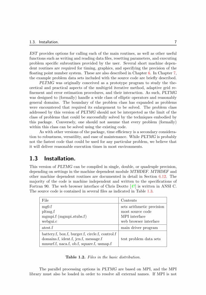
1.3 Installation.This version of PLTMG can be compiled in single, double, or quadruple precision,depending on settings in the machine dependent module MTHDEF. MTHDEF andother machine dependent routines are documented in detail in Section 6.12. Themajority of the code is machine independent and written to the specifications ofFortran 90. The web browser interface of Chris Deotte [47] is written in ANSI C.The source code is contained in several files as indicated in Table 1.3.
File Contents
mg0.f sets arithmetic precisionpltmg.f most source codemgmpi.f (mgmpi stubs.f) MPI interfacewebgui.c web browser interface
atest.f main driver program
battery.f, box.f, burger.f, circle.f, control.fdomains.f, ident.f, jcn.f, message.f test problem data setsmnsurf.f, naca.f, ob.f, square.f, usmap.f
Table 1.2. Files in the basic distribution.
The parallel processing options in PLTMG are based on MPI, and the MPIlibrary must also be loaded in order to resolve all external names. If MPI is not

8 PLTMG USERS’ GUIDE 13.0
available or not desired, one can substitute the supplied stub interface routines.The stub routines are a set of MPI interface routines with all calls to MPI libraryfunctions and subroutines deleted. By using the stub routines in place of the reg-ular interface, one can create an executable with no unresolved external referenceswithout loading the MPI library. In this case, however, all the parallel options ofPLTMG are disabled.
To create an executable, one needs Fortran 90 and C compilers and an MPIinstallation. One should create a test problem data file (myfile.f in the following)or use one of the supplied example test problem data sets. One should compilemg0.f, atest.f, pltmg.f mgmpi.f, myfile.f and webgui.c, and link the resulting objectfiles with the MPI library. One can set most of the usual compiler options asdesired. However, some compilers may require the -pthread option to successfullycompile and link webgui.c. If MPI is not available or not needed, one may substitutemgmpi stubs.f for mgmpi.f as described above.

Chapter 2
Data Structures
2.1 Overview.In this chapter, we define the data structures used in the PLTMG package. Thereare two basic data structures that define the domain Ω: the skeleton and the tri-angulation. Basic to both data structures is the concept of an edge. The varioussubregions that define a skeleton are described by a sequence of edges that traverseits boundary in a counter clockwise fashion. In the case of a triangulation, edgeson the boundary ∂Ω need to be explicitly defined in order to assign boundary con-ditions. Additional internal edges can be defined if they have some attribute ofinterest; e.g., they are curved. Other internal edges are defined implicitly by thedefinitions of the triangles that comprise the triangulation. In the case of parallelprocessing, PLTMG explicitly defines edge data structures for all edges lying on theinternal interface system generated by the partitioning of Ω among the processors.The edge related data structures are defined in Section 2.2. The triangulation andskeleton are defined in Sections 2.3 and 2.4, respectively.
The next few sections define several internal data structures used by PLTMG.The user is never asked to provide data for these structures; they are all computedinternally by various routines in the package. However, their contents may still beof interest to the user. Data structures that track degrees of freedom associatedwith individual elements, as well as the solution and other finite element functions,are described in Section 2.5. The IPATH data structure describes relationshipsbetween the subdomains associated with different processors in a parallel adaptivecalculation. It is described in Section 2.6.
The arrays IP, RP, and SP contain many scalar parameters, switches, controlvariables, flags, and pointers, some that must be specified by the user and othersthat are internally computed but may be of interest to the user. These are describedin Section 2.7. Finally, the coefficient functions defining the differential operatorand functional ρ in (1.1)–(1.3), and the optional function QXY used by TRIGENand TRIPLT, are described in Section 2.8.
9

10 PLTMG USERS’ GUIDE 13.0
2.2 Edge DefinitionsIn this section, we define geometry data structures common to both the triangula-tion and the skeleton. In both cases, the domain is described by a list of vertices vi,1 ≤ i ≤ NVF, and edges bi, 1 ≤ i ≤ NBF. In the case of of a triangulation, the vienumerate all vertices of all triangles that comprise the triangulation. In the case ofa skeleton, the vi enumerate the vertices of all regions that comprise the skeleton.In both cases, the (x, y) coordinates of the vertices are given in the arrays VX andVY . In particular,
vI = (xI , yI) = (VX(I),VY(I)), 1 ≤ I ≤ NVF.
Edges are defined in terms of the integer array IBNDRY of size 7×NBF andthe real array SF of size 2×NBF. The latter is used only for curved edges. Curvededges can be most easily be defined by circular arcs (as in early versions of PLTMG)or parametrically through the function SXY provided by the user. The definitionsof IBNDRY is given in Table 2.1.
Column I of the IBNDRY array contains information about edge bI . The firsttwo entries are pointers to the VX and VY arrays and denote the two vertices thatform the endpoints of the edge. The third entry is used to indicate if the edge iscurved, and is described more fully below.
Entry IBNDRY(4,I) describes the type of boundary conditions to be applied,or if the edge is internal to Ω. A fourth type of edge is a linked edge. Linked edgesoccur only in pairs. If bI and bJ are a pair of linked edges, then IBNDRY(4,I) = −Jand IBNDRY(4,J) = −I. Linked edges bI and bJ must be geometrically congruent.That is, bI must be mapped to bJ using a translation and orthogonal rotation.Continuity of the solution uh and weak continuity of a ·n is imposed on linked edgepairs. Thus if bI and bJ are boundary edges, this is equivalent to imposing periodicboundary conditions. In the course of parallel processing, PLTMG creates edges oftypes 3−5. Entries IBNDRY(5,I) and IBNDRY(6,I) are used internally by PLTMGfor parallel processing.
Entry IBNDRY(7,I) contains an integer label for the edge; this user defined la-bel can be used to uniquely identify a particular edge, or to associate some propertywith the edge.
2.2.1 Curved Edges – Circular Arcs
If a triangle has a curved edge, it can be specified as a circular arc or given a para-metric definition. In the case of a circular arc, one should set IBNDRY(3,I) = 1. Thearc passes through the edge endpoints specified in IBNDRY(1,I) and IBNDRY(2,I)and its center (xc, yc) is specified in the array SF as
(xc, yc) = (SF(1,I),SF(2,I)).
Because there are generally two such arcs for every pair of endpoints, the shorterarc is taken to be the correct edge; therefore, one must specify arcs that subtend(strictly) less than π of arc; π/4 is a reasonable upper bound.

2.2. Edge Definitions 11
array entry definition
IBNDRY(1,I) first endpoint numberIBNDRY(2,I) second endpoint numberIBNDRY(3,I) curved edge switchIBNDRY(4,I) edge typeIBNDRY(5,I) reserved for parallel processingIBNDRY(6,I) reserved for parallel processingIBNDRY(7,I) edge label
IBNDRY definition.
IBNDRY(3,I) curved edge type
0 Straight edge1 Curved edge – circular arc−K Curved edge – parametric
Curved edge types.
IBNDRY(4,I) edge type
2 Dirichlet boundary1 natural boundary0 internal−K linked with edge K
3, 4, 5 reserved for parallel processing
Edge type definitions.
Table 2.1. Boundary definitions and data structures.
To simplify data entry, we provide the routine CENTRE for computing thecenter of a circle given three points on its boundary. CENTRE is called using thestatement
Call CENTRE( X1, Y1, X2, Y2, X3, Y3, XC, YC )
Here (X1,Y1) and (X2,Y2) are the endpoints of an arc of the circle, and (X3,Y3)is a third point on the arc (e.g., the midpoint). CENTRE returns the center of thecircle in (XC,YC).
2.2.2 Curved Edges – Parametric
A second way to specify a curved edge is through a parametric representation. Sincethere may be several parametric curves, they are indexed by the user. In particular,

12 PLTMG USERS’ GUIDE 13.0
if IBNDRY(3,I) = −K, then the parametric function (qK , rK) is used to define theedge, where (
x(s)y(s)
)=
(qK(s)rK(s)
), s1 ≤ s ≤ s2.
The point s = s1 corresponds to the first endpoint and s = s2 corresponds to thesecond. In this case, the values in column I of the array SF are given by
(s1, s2) = (SF(1,I),SF(2,I)).
The parameterization itself is defined by the user in routine SXY. Subroutines SXY,has calling sequence
Call SXY( RL, S, ITAG, VALUES )
Here RL = λ is an input array of size NRL giving the current value of the pa-rameters λ. 1 ≤ NRL ≤ 10 for parameter identification problems, while NRL = 1for the other classes of problems. The parameter s1 ≤ S ≤ s2 is input specifyingthe point where (qK(S), rK(S)) is required. ITAG = K, where K is the input indexof the functional, originally provided by the the user as BNDRY(3,I) = −K. Alsorequired are the derivative values (∂qK/∂s, ∂rK/∂s) and (∂qK/∂λJ , ∂rK/∂λJ) for1 ≤ J ≤ NRL.
The output is provided in the array VALUES, a two dimensional array with2 rows and NRL + 2 columns. To simplify this process, PLTMG supplies a labeledcommon block
common /VAL4/ J0, JS, JL
containing a predefined list of integer pointers mapping function and derivativevalues to particular entries in the VALUES array. The details of this mapping aregiven in Table 2.2.
pointer index VALUES(1, ·) VALUES(2, ·)J0 = 1 J0 qK rKJS = 2 JS qK,s rK,sJL = 3 JL + J − 1 qK,λJ rK,λJ
1 ≤ J ≤ NRL
Table 2.2. VALUES array for subroutine SXY.
It is important to emphasize that the parameterization is assumed to roughlycorrespond to arc length along the curved edge. For example, when the edge isbisected, the “midpoint” (xm, ym) is computed from(
xmym
)=
(qK((s1 + s2)/2)rK((s1 + s2)/2)
).

2.3. The Triangulation. 13
Nodes for isoparametric basis functions are computed using a similar formula. Thequality of such calculations is thus dependent on these user defined parameteriza-tions.
2.3 The Triangulation.In this section, we define the triangulation data structure. Let T denote the tri-angulation consisting of triangles ti, 1 ≤ i ≤ NTF, vertices vi, 1 ≤ i ≤ NVF, andedges bi, 1 ≤ i ≤ NBF. Triangles may have curved edges, as described in Sec-tion 2.2. Curved edges may be on the boundary or in the interior of the region Ω.The ITNODE data structure is a 5×NTF integer array that defines triangles thatcomprise T . The details of this data structure are given in Table 2.3.
array entry definition
ITNODE(1,I) first vertex numberITNODE(2,I) second vertex numberITNODE(3,I) third vertex numberITNODE(4,I) reserved for parallel processingITNODE(5,I) element label
Table 2.3. ITNODE definition for a triangulation.
A given triangle tI ∈ T is specified by giving an accounting of its three ver-tices and by specifying an integer label or tag. The Ith column of the ITNODEarray contains information about tI . The first three entries of ITNODE containthe three vertex numbers of triangle tI . ITNODE(J,I) = K , for 1 ≤ J ≤ 3, means(VX(K),VY(K)) is the Jth vertex of tI . The ordering of the vertices of a given trian-gle is arbitrary and independent of the other triangles.2 Entry ITNODE(4,I) is usedinternally by PLTMG in parallel processing, denoting the processor that “owns” tI ;one can simply initialize ITNODE(4,I) = 0. Entry ITNODE(5,I) contains any userprovided label for tI . Such labels are provided strictly for the convenience of theuser and can be used to identify differing regions or material properties associatedwith the element.
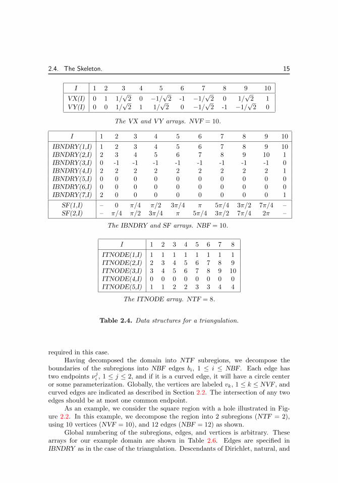
For example, consider the circle of radius one with a crack along the positivex-axis. This domain can be triangulated using NTF = 8 triangles, NVF = 10vertices, and NBF = 10 boundary edges, 8 of which are curved, as illustrated inFigure 2.1. Vertices v2 and v10 have the same (x, y) coordinates, but v2 is “above”the crack and v10 is “below.” Similarly, edge b1 is the top of the crack, while edgeb10 is the bottom. The ordering of vertices, triangles, and edges is arbitrary. In thisexample, we will define the curved edges using the parameterization(
xy
)=
(q1(s)r1(s)
)=
(cos(s)sin(s)
).
2PLTMG reorders vertices as necessary to ensure a counterclockwise orientation for elements.

14 PLTMG USERS’ GUIDE 13.0
Figure 2.1. Clockwise, from upper left: example domain; triangle numbers;vertex numbers; edge numbers.
The data for our example is shown in Table 2.4. In this example, we have chosento label the triangles in ITNODE(5,I) by the quadrant in the Euclidean plane inwhich they lie. In our example, we impose Dirichlet boundary conditions on theouter boundary of the circle, and also along the top of the crack, and Neumannboundary conditions on the bottom of the crack. The outer boundary of the circleis labeled 0, the top of the crack 2, and the bottom of the crack 1.
Several routines in the package check triangulation data structures for commonerrors in the data. If found, such errors are reported by setting the parameterIFLAG as described in Table 2.9.
2.4 The Skeleton.The skeleton data structure is often the easiest data structure for the user to specifyby hand, especially if the domain has complicated geometry, symmetry, or internalinterfaces. In the skeleton data structure, the domain Ω is viewed as the unionof NTF simply connected subregions Ωi, 1 ≤ i ≤ NTF. The regions need not beconvex, and the case NTF = 1 is not excluded. A shared boundary between twosubregions (an internal interface) will be respected by the triangulation process inTRIGEN ; that is, the interface will be represented as one or more triangle edges inthe triangulation.
The boundary of each Ωi should be a simple closed curve that does not in-tersect itself. Thus, for example, if Ω has a hole, adding a single cut between theouter boundary and the hole will not be adequate. At least two subregions will be
2.4. The Skeleton. 15
I 1 2 3 4 5 6 7 8 9 10
VX(I) 0 1 1/√
2 0 −1/√
2 -1 −1/√
2 0 1/√
2 1
VY(I) 0 0 1/√
2 1 1/√
2 0 −1/√
2 -1 −1/√
2 0
The VX and VY arrays. NVF = 10.
I 1 2 3 4 5 6 7 8 9 10
IBNDRY(1,I) 1 2 3 4 5 6 7 8 9 10IBNDRY(2,I) 2 3 4 5 6 7 8 9 10 1IBNDRY(3,I) 0 -1 -1 -1 -1 -1 -1 -1 -1 0IBNDRY(4,I) 2 2 2 2 2 2 2 2 2 1IBNDRY(5,I) 0 0 0 0 0 0 0 0 0 0IBNDRY(6,I) 0 0 0 0 0 0 0 0 0 0IBNDRY(7,I) 2 0 0 0 0 0 0 0 0 1
SF(1,I) – 0 π/4 π/2 3π/4 π 5π/4 3π/2 7π/4 –SF(2,I) – π/4 π/2 3π/4 π 5π/4 3π/2 7π/4 2π –
The IBNDRY and SF arrays. NBF = 10.
I 1 2 3 4 5 6 7 8
ITNODE(1,I) 1 1 1 1 1 1 1 1ITNODE(2,I) 2 3 4 5 6 7 8 9ITNODE(3,I) 3 4 5 6 7 8 9 10ITNODE(4,I) 0 0 0 0 0 0 0 0ITNODE(5,I) 1 1 2 2 3 3 4 4
The ITNODE array. NTF = 8.
Table 2.4. Data structures for a triangulation.
required in this case.Having decomposed the domain into NTF subregions, we decompose the
boundaries of the subregions into NBF edges bi, 1 ≤ i ≤ NBF. Each edge hastwo endpoints νji , 1 ≤ j ≤ 2, and if it is a curved edge, it will have a circle centeror some parameterization. Globally, the vertices are labeled vk, 1 ≤ k ≤ NVF, andcurved edges are indicated as described in Section 2.2. The intersection of any twoedges should be at most one common endpoint.
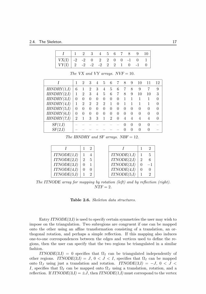
As an example, we consider the square region with a hole illustrated in Fig-ure 2.2. In this example, we decompose the region into 2 subregions (NTF = 2),using 10 vertices (NVF = 10), and 12 edges (NBF = 12) as shown.
Global numbering of the subregions, edges, and vertices is arbitrary. Thesearrays for our example domain are shown in Table 2.6. Edges are specified inIBNDRY as in the case of the triangulation. Descendants of Dirichlet, natural, and

16 PLTMG USERS’ GUIDE 13.0
array entry definition
ITNODE(1,I) first vertex numberITNODE(2,I) first edge numberITNODE(3,I) congruent region numberITNODE(4,I) reserved for parallel processingITNODE(5,I) region label
Table 2.5. ITNODE definition for a skeleton.
Figure 2.2. Example domain decomposed into two subregions (left); vertexnumbers (middle); edge numbers (right).
linked edges are included in the output IBNDRY array when Ω is triangulated usingTRIGEN. Descendants of internal edges are retained only if they separate regionswith different labels or of the edge is curved. Descendant edges inherit the labelof the original edge. In our example, we will assign Dirichlet boundary conditionsto the left and right sides and the bottom of the domain, and natural boundaryconditions elsewhere. The four curved edges are defined by circular arcs of a circlewith its center at the origin. The IBNDRY and SF arrays then have the form givenin Table 2.6.
A subregion Ωi, 1 ≤ i ≤ NTF, is defined by an ordered sequence of edges (atleast three) that form its boundary. The sequence is ordered such that the boundaryof Ωi is traversed in a counterclockwise direction (thus providing notions of “inside”and “outside”). Each edge in the sequence shares exactly one endpoint with theedge that precedes it and the edge that follows it in the sequence; the first and lastedges in the sequence also share one endpoint. A particular edge can appear onlyonce in the sequence.
The array ITNODE is used to define the subregions. Column I of ITNODEcorresponds to the region ΩI . Entry ITNODE(1,I) is a global vertex number forone of the vertices on the boundary of ΩI . Unless ITNODE(3,I) 6= 0 (see below)the choice of vertex is arbitrary. The second entry, ITNODE(2,I), is the global edgenumber of the first edge in a counterclockwise traversal of ΩI , beginning at vertexvK , where ITNODE(1,I) = K.
2.4. The Skeleton. 17
I 1 2 3 4 5 6 7 8 9 10
VX(I) -2 -2 0 2 2 0 0 -1 0 1VY(I) 2 -2 -2 -2 2 2 1 0 -1 0
The VX and VY arrays. NVF = 10.
I 1 2 3 4 5 6 7 8 9 10 11 12
IBNDRY(1,I) 6 1 2 3 4 5 6 7 8 9 7 9IBNDRY(2,I) 1 2 3 4 5 6 7 8 9 10 10 3IBNDRY(3,I) 0 0 0 0 0 0 0 1 1 1 1 0IBNDRY(4,I) 1 2 2 2 2 1 0 1 1 1 1 0IBNDRY(5,I) 0 0 0 0 0 0 0 0 0 0 0 0IBNDRY(6,I) 0 0 0 0 0 0 0 0 0 0 0 0IBNDRY(7,I) 2 1 3 3 1 2 0 4 4 4 4 0
SF(1,I) – – – – – – – 0 0 0 0 –SF(2,I) – – – – – – – 0 0 0 0 –
The IBNDRY and SF arrays. NBF = 12.
I 1 2
ITNODE(1,I) 1 4ITNODE(2,I) 2 5ITNODE(3,I) 0 1ITNODE(4,I) 0 0ITNODE(5,I) 1 2
I 1 2
ITNODE(1,I) 1 5ITNODE(2,I) 2 6ITNODE(3,I) 0 −1ITNODE(4,I) 0 0ITNODE(5,I) 1 2
The ITNODE array for mapping by rotation (left) and by reflection (right).NTF = 2.
Table 2.6. Skeleton data structures.
Entry ITNODE(3,I) is used to specify certain symmetries the user may wish toimpose on the triangulation. Two subregions are congruent if one can be mappedonto the other using an affine transformation consisting of a translation, an or-thogonal rotation, and perhaps a simple reflection. If this mapping also inducesone-to-one correspondences between the edges and vertices used to define the re-gions, then the user can specify that the two regions be triangulated in a similarfashion.
ITNODE(3,I) = 0 specifies that ΩI can be triangulated independently ofother regions. ITNODE(3,I) = J , 0 < J < I, specifies that ΩI can be mappedonto ΩJ using just a translation and rotation. ITNODE(3,I) = −J , 0 < J <I, specifies that ΩI can be mapped onto ΩJ using a translation, rotation, and areflection. If ITNODE(3,I) = ±J , then ITNODE(1,I) must correspond to the vertex

18 PLTMG USERS’ GUIDE 13.0
on ∂ΩI which is mapped to the vertex corresponding to ITNODE(1,J) on ∂ΩJ . IfITNODE(3,I) 6= 0, TRIGEN will map the triangulation generated for ΩJ onto ΩI ,ensuring the desired symmetry properties of the overall triangulation. Note that thisis not a symmetric relation; ITNODE(3,I) = J does not mean ITNODE(3,J) = I.In particular, if | ITNODE(3,I) |≥ I, TRIGEN will return in an error condition.
In our example, Ω2 can be mapped onto Ω1 by either rotation or reflection.We can ensure the triangulation for Ω2 will be similar to that for Ω1, either underrotation or reflection. The resulting triangulations may be different in the twocases.3 ITNODE arrays for the two situations are illustrated in Table 2.6. EntryITNODE(4,I) is used by PLTMG in parallel processing. Entry ITNODE(5,I) is auser defined label for the region; all the triangles created in ΩI inherit this label.
We provide the utility subroutine SKLUTL to aid in the creation of the skele-ton data structures. Subroutine SKLUTL is called using the statement
Call SKLUTL( ISW, VX, VY, SF, ITNODE, IBNDRY, IP,RP, IFLAG, SXY )
This routine takes as input a skeleton data structure defined VX, VY, SF,IBNDRY, (except when ISW = 0) ITNODE, and the routine SXY, called if curvededges are defined by a parameterization. The integers NTF, NBF, and (except whenISW = 0) NTF should be specified in the IP array, and λ = RL should be specifiedin RP if SXY is to be called. The integer ISW specifies the task, as indicated inTable 2.7.
ISW task
0 create ITNODE array1 refine long circular arcs2 determine congruent regions
Table 2.7. The values of ISW.
If ISW = 0, SKLUTL computes all entries of the ITNODE array, given theremaining arrays in the skeleton data structure (VX, VY, SF, and IBNDRY ), andthe parameters NVF, and NBF in the IP array. The value of NTF is returned inthe IP array. The regions are labeled with ITNODE(5,I) = I for 1 ≤ I ≤ NTF,although these labels can subsequently be reset by the user. Also ITNODE(3,I) = 0for 1 ≤ I ≤ NTF. If ISW = 1, SKLUTL accepts as input a complete skeletondescription, and divides curved edges defined as circular arcs as necessary to ensurethat all such edges subtend less than π/4 of arc. New edges and vertices are addedas necessary, and the relevant skeleton parameters updated. New values of NBF andNVF are returned in the IP array. If ISW = 2, SKLUTL accepts as input a completeskeleton description, and finds congruent regions. The values of ITNODE(3,I) (and
3 We could ensure greater symmetry in the triangulation by decomposing Ω into 4 or 8 congruentregions instead of 2 and then setting ITNODE(3,I) appropriately.

2.5. Finite Element Data Structures. 19
possibly ITNODE(1,I) and ITNODE(2,I)) are reset as necessary. If two regions arecongruent but the congruence is not unique, as in our example, an arbitrary choiceis made from among the possibilities. Errors are returned in the integer IFLAG asdescribed in Table 2.9.
Several other routines in the package check skeleton data structures for com-mon errors in the data. If found, such errors are reported by setting the parameterIFLAG as described in Table 2.9.
2.5 Finite Element Data Structures.Several data structures in PLTMG define and maintain the finite element functionsassociated with a particular problem. In particular, the 8 × NTF integer arrayITDOF contains information about polynomial spaces on each element, the realarray GF contains the numerical values of the solution and other finite elementfunctions, and the real array E contains information about the a posteriori errorestimates in each element. These data structures are not defined or initialized bythe user, but it may be of interest for a user to understand their contents.
PLTMG uses local notation to define certain quantities related to a givenelement in the mesh. See Figure 2.3. For example, each element locally has verticeslabeled νk, 1 ≤ k ≤ 3. From this viewpoint, the ITNODE array contains a mappingfor these locally defined vertices to globally defined vertices, with νK correspondingto ITNODE(K, ·) for 1 ≤ K ≤ 3. Edges are locally labeled as in Figure 2.3, withedge εk opposite vertex νk, 1 ≤ k ≤ 3.
AAAAAAAAAA
ν1 ν2
ν3
ε1ε2
ε3
tI
Figure 2.3. Local notation for element tI .
In the ITDOF array, column I contains information related to element tI .The first three entries give the global indices for the degrees of freedom associatedwith the three vertices of the the element. If the element has an edge with degreep ≥ 2 there are p − 1 degrees of freedom (bump functions) associated with thatedge. In PLTMG these degrees of freedom are given consecutive global indices,that either increase or decrease with a counter clockwise traversal of that edge.Entries 4–6 in column I provide the starting degree of freedom for each edge, witha sign that indicates whether they increase or decrease. If the element has degree

20 PLTMG USERS’ GUIDE 13.0
array entry definition
ITDOF(1,I) degree of freedom for vertex ν1
ITDOF(2,I) degree of freedom for vertex ν2
ITDOF(3,I) degree of freedom for vertex ν3
ITDOF(4,I) ± first degree of freedom for edge ε1ITDOF(5,I) ± first degree of freedom for edge ε2ITDOF(6,I) ± first degree of freedom for edge ε3ITDOF(7,I) first interior degree of freedom for element tIITDOF(8,I) polynomial degrees for element tI
Table 2.8. ITDOF definition.
p ≥ 3 there are (p − 1)(p − 2)/2 degrees of freedom (bubble functions) associatedwith the element interior. These are also given consecutive global indices. Thelowest numbered corresponds to the interior node closest to vertex ν1; subsequentlythey are numbered “row-by-row;” within each row, degrees of freedom are numbered“left-to-right” with the lowest number for that row corresponding to the node closestto edge ε3. The global index for the lowest numbered interior degree of freedom isgiven in ITDOF(7,I).
Entry ITDOF(8,I) contains information about the degree of the polynomialsassociated with element tI . Let the element itself have degree p0. Each edge εk canhave a different degree pk ≥ p0, 1 ≤ k ≤ 3. In PLTMG, elements and edges canhave degree at most nine.4 These degrees are encoded in ITDOF(8,I) as
ITDOF(8,I) = p0 + 16p1 + 162p2 + 163p3.
The total number of degrees of freedom associated with the finite elementspace is NDF. Values for finite element functions are stored in the array GF, withMAXD ≥ NDF rows and 1 ≤ I ≤ 13 columns, depending on the problem, witheach column associated with a specific finite element function. The definitions foreach problem are given in Table 2.9.
The first column of GF always contains the finite element solution u. If theproblem is solved via parallel computation, then the last column of GF contains thefunction ω, which is a locally computed dual function that indicates the influenceof the regions outside of the given processor’s assigned domain on that domain.For simple pde equations, the user can also specify a functional computed from theuser supplied function ρ. For continuation problems, the tangent vector u, as wellas u0 and u0 from the previous step, are stored. The vectors ψr and ψ` are theright and left singular vectors, respectively, associated with the smallest singularvalue of the Jacobian (stiffness) matrix; these are used in the determination oflimit and bifurcation points, among other things. Parameter identification andoptimal control problems require a Lagrange multiplier function v. The optimal
4This constraint is due to limitations of available quadrature rules, given by Zhang, Cui, andLiu in [67], and not to any intrinsic constraint on the spaces themselves.

2.6. Parallel Processing Data Structure. 21
problem 1 2 3 4 5 6 7
simple pde u (ud) (ω)obstacle problem u (ω)continuation problem u u0 u u0 ψr ψ` (ω)parameter identification u v uλ1
(ω)distributed control u v λ (ω)
Table 2.9. GF data structure definitions. Columns labeled I, 1 ≤ I ≤ 7,refer to the function stored in GF(·, I). Functions appearing within parenthesesare computed only in certain situations. For the parameter identification problem,columns 2 + J , 1 ≤ J ≤ NRL, contain uλJ and column 3 + NRL contains ω ifpresent.
control problem also requires the distributed control function λ, and the parameteridentification problem requires NRL vectors uλk for 1 ≤ k ≤ NRL.
The array E contains information about a posteriori error estimates. It hasMAXT ≥ NTF rows and two columns. The first column contains the local errorindicator ηI for element tI , and the second column contains a normalization constantused in the decision process in hp refinement. We note that information in the Earray is typically modified by various adaptive algorithms in TRIGEN, and theoutput from TRIGEN in the E array should be considered unreliable except in thecase when TRIGEN is called to only compute error estimates.
2.6 Parallel Processing Data Structure.When PLTMG solves a problem using parallel processing, it partitions the domainΩ into NPROC subdomains ΩI if NPROC processors are used. This creates aninternal interface system Γ; PLTMG creates internal edges as needed such thatevery edge in the internal interface system is represented in the IBNDRY array. Atthe conclusion of the adaptive process, the global conforming finite element spaceneeds to be created, and corresponding edges and degrees of freedom on differentprocessors need to be linked in order to carry out the domain decomposition solvethat computes the final finite element solution on the global mesh.
The integer array IPATH is a data structure jointly computed by all of theprocessors; each processor provides a block of data within the IPATH array thatdescribes its part of the global interface system. In particular, each processor be-gins its adaptive enrichment starting from the same interface system, consisting ofso-called root edges. Root edges my be bisected (h-refined) or have their degreeincreased (p-refined) in potentially arbitrary combinations. The data in the IPATHarray provides a binary tree for each root edge, as well as pointers that indicate theglobal edge numbers and degrees of freedom for that edge in that processors owndata structures. Data for different types of nodes in the tree is given in Table 2.10.
The IPATH array has six rows. For all edges in the tree, the first entry

22 PLTMG USERS’ GUIDE 13.0
array entry root root/leaf internal leaf
IPATH(1,I) neighbor neighbor neighbor neighborIPATH(2,I) child -edge child -edgeIPATH(3,I) – vertex 1 – vertex 1IPATH(4,I) – vertex 2 – vertex 2IPATH(5,I) – ± edge – ± edgeIPATH(6,I) – degree – degree
Table 2.10. IPATH definition – tree section.
(neighbor) is a pointer to the column in IPATH that contains the same edge, butfor the neighbor processor; this is the key that identifies the same physical edge ondifferent processors. The second entry identifies the (first) child for non-leaf edgesin the tree; these are just pointers to other columns in the IPATH array. The twochildren of a bisected edge appear in consecutive columns in IPATH. Leaf entrieshave a pointer (-edge) that points to the column corresponding to that edge in thegiven processors IBNDRY array; the negative sign is to distinguish it from a childpointer.
In the domain decomposition solve, interface information corresponding to allnodes lying on the global interface system must be exchanged via MPI. This isdone using a transient interface data structure, with blocks of data provided byeach processor. Entries 3–6 in the IPATH array for leaf edges provide pointers thatindicate the location in the transient data structure for data corresponding to thetwo endpoints, and if the edge degree p ≥ 2, the edge data. The fifth location isstored as ±edge, with the sign indicating a increase or decrease in index with acounter clockwise traversal.
The first NPROC + 2 columns of the IPATH data structure contain pointers,one column for each processor, one column for the global mesh and one columnfor the coarse part of the interface of the given processor. These pointers indicatethe blocks of the IPATH array and the shared array for the domain decompositionsolver that are used by the given processor. Note that after the basic IPATH arrayis computed jointly by all of the processors, each processor appends a tree sectionfor the coarse part of its interface to the end of the IPATH array. This informationis different on every processor and is used by the domain decomposition solver.
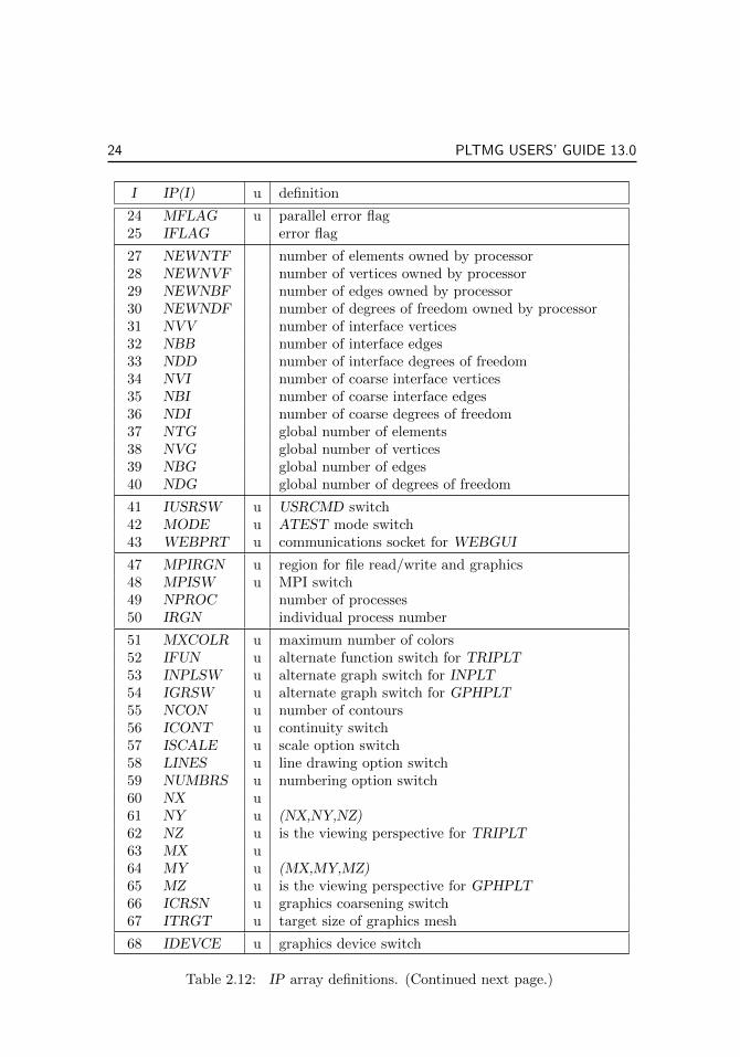
2.7 Parameter Arrays.IP, RP, and SP are integer, real, and CHARACTER*80 arrays, respectively, oflength 100 containing various user specified parameters, and internally generatedparameters, switches, flags, and pointers. A list of the currently used locations,their names, and brief definitions appears in Tables 2.12–2.14. Parameters marked“u” should be supplied by the user.
The parameter IFIRST is an initialization switch specifying the degree of the

2.7. Parameter Arrays. 23
IFIRST option
0 no initialization1 initialize for piecewise linear elements2 initialize for piecewise quadratic elements3 initialize for piecewise cubic elements4 initialize for piecewise quartic elements5 initialize for piecewise quintic elements6 initialize for piecewise polynomials of degree 67 initialize for piecewise polynomials of degree 78 initialize for piecewise polynomials of degree 89 initialize for piecewise polynomials of degree 9
Table 2.11. The values of IFIRST.
finite element space to be used, as indicated in Table 2.11. If IFIRST = 0, noinitialization takes place. If IFIRST = p, 1 ≤ p ≤ 9, triangulation data structuresare checked, and various arrays are initialized for piecewise polynomial elements ofdegree p. Array entry IP(25) is the error flag IFLAG. A summary of the possiblevalues for IFLAG is given in Table 2.15.
I IP(I) u definition
1 NTF u number of triangles / regions2 NVF u number of vertices3 NBF u number of edges4 NDF u number of degrees of freedom5 IFIRST u initialization switch6 IPROB u problem type7 ITASK u problem task8 ISPD u symmetric / nonsymmetric switch9 METHOD u preconditioner options10 MXCG u maximum conjugate gradient iterations11 MXNWTT u maximum damped Newton iterations12 ISING u switch for singular Neumann problem13 NRL u number of parameters λ
17 IRTYPE u refinement / coarsening options18 MXORD u maximum polynomial degree19 IERRSW u error recovery switch20 IADAPT u mesh generation option switch21 IREFN u uniform refinement control22 NDTRGT u target value for number of vertices
23 NOCHNG u PLTMG-TRIGEN communication flag
Table 2.12: IP array definitions. (Continued next page.)
24 PLTMG USERS’ GUIDE 13.0
I IP(I) u definition
24 MFLAG u parallel error flag25 IFLAG error flag
27 NEWNTF number of elements owned by processor28 NEWNVF number of vertices owned by processor29 NEWNBF number of edges owned by processor30 NEWNDF number of degrees of freedom owned by processor31 NVV number of interface vertices32 NBB number of interface edges33 NDD number of interface degrees of freedom34 NVI number of coarse interface vertices35 NBI number of coarse interface edges36 NDI number of coarse degrees of freedom37 NTG global number of elements38 NVG global number of vertices39 NBG global number of edges40 NDG global number of degrees of freedom
41 IUSRSW u USRCMD switch42 MODE u ATEST mode switch43 WEBPRT u communications socket for WEBGUI
47 MPIRGN u region for file read/write and graphics48 MPISW u MPI switch49 NPROC number of processes50 IRGN individual process number
51 MXCOLR u maximum number of colors52 IFUN u alternate function switch for TRIPLT53 INPLSW u alternate graph switch for INPLT54 IGRSW u alternate graph switch for GPHPLT55 NCON u number of contours56 ICONT u continuity switch57 ISCALE u scale option switch58 LINES u line drawing option switch59 NUMBRS u numbering option switch60 NX u61 NY u (NX,NY,NZ)62 NZ u is the viewing perspective for TRIPLT63 MX u64 MY u (MX,MY,MZ)65 MZ u is the viewing perspective for GPHPLT66 ICRSN u graphics coarsening switch67 ITRGT u target size of graphics mesh
68 IDEVCE u graphics device switch
Table 2.12: IP array definitions. (Continued next page.)

2.7. Parameter Arrays. 25
I IP(I) u definition
69 FPANE u WEBGUI canvas for TRIPLT70 GPANE u WEBGUI canvas for GPHPLT71 JPANE u WEBGUI canvas for INPLT
73 MXLABL maximum label for MPI interface edges74 NVDD total number of interface vertices75 LIPATH length of IPATH array76 NEF number of error functions77 NGF number of grid functions78 NDL order of error recovery systems79 IEVALS number of function evaluations on last call80 ITNUM number of Newton iterations on last call
82 MAXPTH u number of columns in the array IPATH83 MAXT u number of columns in the array ITNODE84 MAXV u length of the arrays VX and VY85 MAXD u length of grid function array GF86 MAXB u number of columns in the array IBNDRY
90 NDF order of the linear system91 NB number of blocks in the linear system92 LENJA length of JA array93 LENAD length of diagonal part A array94 LENAOD length of upper / lower triangular A array95 LENJU maximum length of JU array96 LENUOD maximum length of upper / lower triangular U array97 LENJU0 length of JU array98 LENU0 length of U array99 LENJA0 length of JA for HB decomposition100 LENJUC length of JU for HB decomposition
Table 2.12: IP array definitions.
I RP(I) u definition
1 RLTRGT u target value for λ2 RTRGT u target value for ρ(u, λ)3 RMTRGT u target value for µ4 DTOL u drop tolerance for incomplete factorization6 SMIN u lower limit for contour colors7 SMAX u upper limit for contour colors8 RMAG u window magnification factor9 CENX u (CENX,CENY) are the window center coordinates
Table 2.13: RP array definitions. (Continued next page.)

26 PLTMG USERS’ GUIDE 13.0
I RP(I) u definition
10 CENY u12 HMAX u approximate largest element size13 GRADE u largest growth factor for adjacent elements14 HMIN u approximate smallest edge length
16 XMIN17 XMAX Ω ⊂ (XMIN,XMAX)× (YMIN, YMAX)18 YMIN19 YMAX
21 RL current value of λh22 R current value of ρ(uh, λh) = ρh23 RLDOT current value of λh24 RDOT current value of ρh25 SVAL current value of smallest singular value26 RLSTRT starting value for λh27 RSTRT starting value for ρ(uh, λh)
31 RL0 previous value of λh32 R0 previous value of ρ(uh, λh) = ρh33 RL0DOT previous value of λh34 R0DOT previous value of ρh35 SVAL0 previous value of smallest singular value
37 ENORM1 estimate for ||u− uh||H1(Ω)
38 UNORM1 the norm ||uh||H1(Ω)
39 ENORM2 estimate for ||u− uh||L2(Ω)
40 UNORM2 the norm ||uh||L2(Ω)
41 RELERP relative size of solution error ||eh||H1(ΩI)/||uh||H1(ΩI)
42 EAVE2 arithmetic average of ||eh||2H1(t)
52 STEP damping step s for Newton’s method53 RELER0 relative size of solution error ||eh||H1(Ω)/||uh||H1(Ω)
54 RELERR relative size of Newton update ||δU ||/||U ||55 ANORM maximum diagonal entry in Jacobian matrix56 RELRES the relative residual ||Gk||/||G0||57 BRATIO the relative residual ||Gk||/||Gk−1||58 DNEW the discrete inner product −〈GuδU,G〉59 BNORM0 scaling factor ||G0||60 BMNRM0 scaling factor for ρ63 RMU current value of interior point parameter µ64 REG4 internal regularization parameter for IPROB = 465 REG5 internal regularization parameter for IPROB = 5
67 SCLEQN current value of scalar equation N − σ68 SCALE scaling factor for scalar equation
Table 2.13: RP array definitions. (Continued next page.)

2.7. Parameter Arrays. 27
I RP(I) u definition
69 THETAL (2− θ)λh in scalar equation70 THETAR θρh in scalar equation71 SIGMA the step σ for scalar equation72 DELTA Newton update for λh73 DRDRL the value of ∂ρ/∂λ
74 SEQDOT the value of N
76 QUAL target element quality77 ANGMN target minimum angle78 DIAM approximate diameter of Ω79 BEST value of TRIGEN quality function80 AREA area of Ω
82 N0 degrees of freedom for region ΩI83 E0 error for region ΩI84 NF global degrees of freedom85 EF global error
91 RL1 value of λ1
92 RL2 value of λ2
93 RL3 value of λ3
94 RL4 value of λ4
95 RL5 value of λ5
96 RL6 value of λ6
97 RL7 value of λ7
98 RL8 value of λ8
99 RL9 value of λ9
100 RL10 value of λ10
Table 2.13: RP array definitions.
I SP(I) u definition
1 ITITLE u title for INPLT2 FTITLE u title for TRIPLT3 GTITLE u title for GPHPLT4 LOGO u title for web browser tab
5 GRFILE u file for hard copy graphics output6 RWFILE u save file for read/write commands7 JRFILE u read file for journal command8 JWFILE write file for journal command9 BFILE u output file10 JTFILE temporary file for journal command
Table 2.14: SP array definitions. (Continued next page.)

28 PLTMG USERS’ GUIDE 13.0
I SP(I) u definition
11 IOMSG error message string12 CMD current command string
Table 2.14: SP array definitions.
PLTMG has seven labeled common blocks:
common /pltmg1/ic(3,363),jc(12)
common /pltmg2/c(2,78),wt(78),np1(13)
common /pltmg3/c(3,746),wt(746),np2(22)
common /pltmg4/fc(2541)
common /pltmg5/cb(65,65),cd(12,65),cs(12,45),iptr(12),jptr(12)
common /pltmg6/path(101,6)
common /pltmg7/time(3,50),hist(22,30)
Common block PLTMG1 contains basic definitions of the family of finite ele-ments. Blocks PLTMG2 and PLTMG3 contain definitions of quadrature rules forone dimensional integrals on intervals (Gauss Quadrature), and two dimensionalintegrals on triangles, from Zhang, Cui, and Liu, [67]. Block PLTMG4 contains in-formation used in the two level HB solver described in Section 4.3. Block PLTMG5contains information used in the evaluation of basis functions on transition ele-ments. Block PLTMG6 collects data on various aspects of continuation problems,IPROB = 3 (See Section 4.6). Block PLTMG7 collects statistical data on variousaspects of the calculation.
2.8 Coefficient Functions.Several routines in the package require knowledge of the partial differential equation(1.1), the boundary conditions (1.2), the functional ρ in (1.3), and, on occasion, analternate function of the solution. This information is provided by the user throughsubroutines A1XY, A2XY, FXY, GNXY, GDXY, P1XY, P2XY, and QXY .
Subroutines A1XY, A2XY, FXY, and P1XY have identical argument lists.
Call A1XY( X, Y, U, UX, UY, RL, ITAG, VALUES ),Call A2XY( X, Y, U, UX, UY, RL, ITAG, VALUES ),Call P1XY( X, Y, U, UX, UY, RL, ITAG, VALUES ),Call FXY( X, Y, U, UX, UY, RL, ITAG, VALUES ).
In these subroutines, all of the arguments except VALUES are provided as

2.8. Coefficient Functions. 29
IFLAG general return codes
0 normal return25 wrong input data structure
IFLAG PLTMG and TRIGEN errors
1 zero pivot in sparse factorization2 Newton method line search failed5 solution zero; cannot compute error estimate6 illegal problem type7 continuation procedure failed10 multigraph iteration failed to converge11 Newton (Newton/DD) iteration failed to converge24 Error on one or more MPI processes48 MPI was off for a command needing MPI49 NPROC > NTF in load balance71 no interface unknowns in DD solver72 IPATH array not created
IFLAG storage errors
82 storage exhausted in array IPATH83 storage exhausted in arrays ITNODE and ITDOF84 storage exhausted in arrays VX and VY85 storage exhausted in array GF86 storage exhausted in arrays IBNDRY and SF
IFLAG data errors for triangulation
−31 illegal ITNODE(K,*) K = 1, 2, 3−32 overlapping triangles in ITNODE
IFLAG data errors for triangulation and skeleton
−40 illegal value for NVF, NTF, or NBF−41 illegal IBNDRY(K,*) K = 1, 2−42 illegal IBNDRY(3,*)−43 illegal IBNDRY(4,*)−44 incorrect circle center coordinates−45 arc greater than π/2 in length−46 error in linked edges−47 boundary vertex without two boundary edges−48 ITNODE and IBNDRY are not consistent
IFLAG data errors for skeleton
−51 illegal ITNODE(1,*)−52 illegal ITNODE(2,*)−53 skeleton tracing error−54 region specified in clockwise order−55 illegal ITNODE(3,*)
Table 2.15. Error flag values.

30 PLTMG USERS’ GUIDE 13.0
input. In particular (X,Y ) ∈ Ω is the evaluation (quadrature) point, and
U = uh(X,Y ),
UX =∂uh∂x
(X,Y ),
UY =∂uh∂y
(X,Y ),
RL = λh,
For the parameter identification problem, RL is an array for size NRL with the valueof the vector λh, and for the distributed control problem, RL = λh(X,Y ). Theparameter ITAG=ITNODE(5,I) is the user specified label associated with elementτI ∈ T containing (X,Y ). From this input data, the user provides values of thegiven function and its derivatives in the array VALUES. This array is of size 4+NRL.All entries are initially set to zero by the calling routine; thus the user need supplyonly nonzero values.
To simplify this process, PLTMG supplies a labeled common block
common /VAL0/ K0, KU, KX, KY, KL
containing a predefined list of integer pointers mapping function and derivativevalues to particular entries in the VALUES array. The details of this mapping aregiven in Table 2.16 for the case of f ; the identical mapping is used for a1, a2 andp1.
pointer index VALUES(·)K0 = 1 K0 fKU = 2 KU fuKX = 3 KX fuxKY = 4 KY fuyKL = 5 KL + J − 1 fλJ
1 ≤ J ≤ NRL
Table 2.16. VALUES array for subroutine FXY.
For example, if
f = λ∂u
∂x+ u2,
then the following code fragment would be included in Subroutine FXY.
VALUES(K0)= RL * UX + U**2VALUES(KX)= RLVALUES(KU)= 2 * UVALUES(KL)= UX

2.8. Coefficient Functions. 31
The subroutine corresponding to p2 is P2XY and is called using
Call P2XY( X, Y, DX, DY, U, UX, UY, RL, ITAG, JTAG, VALUES ).
The arguments are a superset of those of the previous subroutines, and all ar-guments with the same name serve the same purpose. This routine is called onlywith points (X,Y ) lying on some edge eJ ∈ Γ. The additional arguments (DX,DY )are the unit normal direction for the edge, and JTAG=IBNDRY(7,J) is the userspecified label for the given edge. The mapping given in Table 2.16 is used here aswell.
The subroutine corresponding to g1 is GNXY and is called using
Call GNXY( X, Y, U, RL, ITAG, VALUES ).
This routine is called only for points (X,Y ) ∈ ∂Ω1, and as in the previous cases, allarguments except the array VALUES are input. In this case ITAG=IBNDRY(7,I)is the user supplied label for the edge, and VALUES is an array of size 2 + NRL.Here the labeled common block
common /VAL1/ K0, KU, KL
assists in mapping function and derivative values to particular entries in the VAL-UES array. The details of the mapping are given in Table 2.17.
pointer index VALUES(·)K0 = 1 K0 gKU = 2 KU guKL = 3 KL + J − 1 gλJ
1 ≤ J ≤ NRL
Table 2.17. VALUES array for subroutine GNXY.
The subroutine corresponding to g2 is GDXY and is called using
Call GDXY( X, Y, RL, ITAG, VALUES ).
This routine also supplies the upper and lower bounds for the inequality constraintson uh for the obstacle problem, bounds on λh in the case that λ = λ(x, y), andthe initial guess u0, for the solution uh. For parameter identification problems, theLagrange multiplier can be initialized using v0, and for optimal control problemsthe Lagrange multiplier can be initialized with v0 and λ(x, y) can be initializedwith λ0. When called to supply a Dirichlet boundary condition, (X,Y ) ∈ ∂Ω2 andITAG=IBNDRY(7,I) is an edge label. When called in regard to inequality con-straints and the initial guess, (X,Y ) ∈ Ω and ITAG=ITNODE(5,I) is the element

32 PLTMG USERS’ GUIDE 13.0
label supplied by the user. Similar to the other routines, VALUES is an outputarray of size 3 + 4NRL. It’s entries can be conveniently accessed through pointersprovided in the labeled common block
common /VAL2/ K0, KL, KLB, KUB, KIC, KIM, KIL
The details are provided in Table 2.18.
pointer index VALUES(·)K0 = 1 K0 gKL = 2 KL + J − 1 gλJ
KLB = 2 + NRL KLB + J − 1 u, λJKUB = 2 + 2NRL KUB + J − 1 u, λJKIC = 2 + 3NRL KIC u0
KIM = 3 + 3NRL KIM v0
KIL = 4 + 3NRL KIL + J − 1 λ0,J
1 ≤ J ≤ NRL
Table 2.18. VALUES array for subroutine GDXY.
Subroutine QXY is
Call QXY( X, Y, U, UX, UY, RL, ITAG, VALUES)
This routine provides the alternate function to display in TRIPLT and the alternatefunction for adaptive algorithms in TRIGEN. The arguments are defined as in theother coefficient functions. The output array VALUES has dimension 4; It’s entriescan be conveniently accessed through pointers provided in the labeled common block
common /VAL3/ KF, KF1, KF2, KAD
whose entries are documents in Table 2.19.
pointer index VALUES(·)K0 = 1 K0 alternate scalar function for TRIPLTKF1 = 2 KF1 first component of vector function for TRIPLTKF2 = 3 KF2 second component of vector function for TRIPLTKAD = 4 KAD alternate function for adaptive algorithms in TRIGEN
Table 2.19. VALUES array for subroutine QXY
In the case of a singular Neumann problem (e.g., a1 ≡ ux, a2 ≡ uy, f ≡ 0,and ∂Ω1 = 0 in (1.1)), the solution u not unique but is determined only up to an

2.9. Sparse Matrix Storage. 33
arbitrary constant. Setting the switch ISING = 1 causes both right hand sides andsolutions in all linear systems to be orthogonalized with respect to constants, ineffect computing least squares solutions in the orthogonal complement subspace. Inother situations, one should set ISING = 0.
2.9 Sparse Matrix Storage.Although sparse matrices are presently generated internally within PLTMG, it maystill be of interest to understand the data structures involved. This version ofPLTMG uses two variants of a basic sparse matrix data structure – a point version,where matrix elements are simple scalar values, and a block version where matrixelements are allowed to be blocks of arbitrary size. The block version is of interest,since the degrees of freedom associated with a single edge or element interior forma so-called clique within the graph of the matrix. These correspond to dense blockswithin the sparse matrix if all members of a clique are ordered consecutively, asis the case here. Taking advantage of these dense blocks can reduce the integeroverhead and indirect addressing associated with processing those cliques.
We begin discussion with the point version of the data structure. Here matricesare stored in the sparse matrix format described in [5] using an integer array JAand a real array A. As an example, consider the 4× 4 matrix given by
A =
a11 a12 a14
a21 a22 a23 a24
a32 a33
a41 a42 a44
. (2.1)
This matrix is stored in JA and A as illustrated in Table 2.20. All nonzeros arestored in the array A. First the diagonal entries are stored, followed by the uppertriangular entries, stored row by row. If the matrix is nonsymmetric, this is fol-lowed by the lower triangular entries, stored column by column. Symmetric andnonsymmetric storage is governed by the parameter ISPD as indicated in Table2.20.
ISPD storage/iteration options
0 nonsymmetric/biconjugate gradient1 symmetric/conjugate gradient
Table 2.20. The values of ISPD.
The first NDF + 1 entries of JA are pointers. In particular, entries JA(I)to JA(I+1) − 1 of the JA array contain column indices for nonzeros in row I ofthe strict upper triangle. As illustrated in Table 2.21, the column indices standin correspondence to the nonzeros of the upper triangle stored in the array A. Ifnonsymmetric storage is used, entries of the transposed lower triangle are stored inthe same order as the upper triangle.

34 PLTMG USERS’ GUIDE 13.0
I 1 2 3 4 5 6 7 8 9 10 11 12 13
JA(I) 6 8 10 10 10 2 4 3 4A(I) a11 a22 a33 a44 − a12 a14 a23 a24 a21 a41 a32 a42
Table 2.21. Sparse matrix data structures. JA has 9 entries. A has 9entries if ISPD = 1 or 13 entries if ISPD = 0.
Now suppose the elements aii in (2.1) are ki × ki square matrices. Then theoff-diagonal blocks ai,j are ki × kj rectangular blocks. Suppose that there are NBblocks, where
NDF =
NB∑i=1
ki
The JA array for the block case is identical to the point case, except that nowentries refer to block rows and columns rather than individual elements. This couldbe much smaller that the point version of the JA array. For example, a mesh withNVF vertices and all elements of degree p will have approximately NDF ≈ p2NVFdegrees of freedom and a point JA array with O(p4NVF) entries. On the otherhand, for this case NB ≈ 6×NVF, and the corresponding block JA array will haveabout 39×NVF entries.
Additionally we need an array IBS of size NB to indicate the sizes of thediagonal blocks
IBS(I) = kI 1 ≤ I ≤ NB.
The A array in this case is more complicated. Following the pattern of thescalar case, we store the diagonal blocks first, followed by the upper triangularblocks, stored (block) row-wise. If ISPD = 0, the upper triangle is followed by thelower triangular block, stored (block) column-wise. The individual diagonal blocksare stored in the same pattern; the diagonal stored first, followed by the uppertriangle, stored row-wise, and if ISPD = 0, this is followed by the lower trianglestored column-wise. The upper triangular blocks are stored row-wise, and the lowertriangular blocks, if present, are stored column-wise.
To access this data, we need an additional integer array JAP of pointers,where JAP(I) indicates the location in the A array where the block correspondingto JA(I) begins. This array is the same size as JA (plus one for convenience).
For the case ISPD = 1, JAP(1) = 1 and
JAP(I+1) = JAP(I) + IBS(I) × (IBS(I) + 1)/2,
while for ISPD = 0
JAP(I+1) = JAP(I) + IBS(I)2,
for 1 ≤ I ≤ NB. Note that the value of JAP(NB+1) is defined. For the uppertriangle, we have JAP(NB+2) = JAP(NB+1). For I = 1, 2, . . .NB and JA(I) ≤

2.9. Sparse Matrix Storage. 35
K ≤ JA(I+1) − 1, we have
JAP(K+1) = JAP(K) + IBS(I) × IBS(JA(K)).
The array JAP can be computed once and saved, but we prefer to computeit as needed from the IBS and JA arrays. Some of our problem classes involveseveral sparse matrices, some symmetric and some nonsymmetric. For this case, oneinstance of the IBS and JA arrays can be used for all sparse matrices, independentof their symmetry, and routines that need JAP (e.g, a routine to compute a matrix-vector multiply) can compute it based on the symmetry status of the particularmatrix involved.
Data structures JU and U are analogous to JA and A, respectively, and con-tain the (incomplete) A ≈ LDU factorization, where D is (block) diagonal, U isunit (block) upper triangular, and L is unit (block) lower triangular, with Lt = Uif At = A.

36 PLTMG USERS’ GUIDE 13.0

Chapter 3
Mesh Generation
3.1 Overview.Subroutine TRIGEN creates or adaptively modifies the data structures defining theregion Ω. There are options to generate a triangulation from a skeleton, adaptivelyrefine or unrefine a triangulation, uniformly refine a triangulation, and adaptivelysmooth the vertices of a triangulation. TRIGEN also has several options for parti-tioning and mesh management in parallel computation environments. The param-eter IADAPT specifies various options for TRIGEN, summarized in Table 3.1.
TRIGEN is called using the statement
Call TRIGEN( VX, VY, SF, ITNODE, IBNDRY, ITDOF, IPATH,E, IP, RP, SP, IU, RU, SU, GF, QXY, SXY )
Except for the case IADAPT = 5, on input the arrays VX, VY, SF, ITNODE,and IBNDRY should define a triangulation. For IADAPT = 5, the input shouldbe a skeleton. The arrays IU, RU, and SU are broadcast and received in MPIcommunication steps, but are not directly used in TRIGEN. When TRIGEN isused to adaptively modify an existing triangulation the procedures generally relyon local a posteriori error estimates for the finite element approximation, althoughsome options are provided for adaptation based on other functions.
If IADAPT = −K for 1 ≤ k ≤ 3, the refinement and/or unrefinement oradaptive mesh smoothing processes are carried out using interpolation errors forthe function QXY in place of the a posteriori error estimates. In particular, for agiven element t of degree p, let qp+1 denote the interpolating polynomial for QXYof degree p+ 1, characterized by nodes at the usual Lagrange lattice points of t. Inthis situation, we can use the (constant) derivatives of order p+ 1 of qp+1 in placeof the corresponding recovered derivatives for uh. Once this substitution is made,the adaptive algorithms proceed in the usual fashion.
We do not anticipate that this option will be used much; it was originally im-plemented to allow subroutine TRIGEN to be debugged independently of subrou-
37

38 PLTMG USERS’ GUIDE 13.0
IADAPT mesh generation option
0 error estimates only1 refine or unrefine mesh using uh-1 refine or unrefine mesh using QXY2 unrefine and refine mesh using uh-2 unrefine and refine mesh using QXY3 smooth mesh points using uh-3 smooth mesh points using QXY4 uniform mesh refinement-4 uniform degree refinement5 skeleton → triangulation
6 load balance (MPI)7 reconcile mesh (MPI)
Table 3.1. Some options use a posteriori error estimates for the computedsolution uh or interpolation errors for the alternative function QXY. Other optionsrequire MPI for parallel communication.
tine PLTMG. On the other hand, there may be special cases where some functionalother than the a posterior error estimate for ||∇(u− uh)||L2(t) should be optimized.Note that if TRIGEN is called before a solution uh is computed by PLTMG, valuesof the arguments U , UX, UY , and RL provided by TRIGEN to QXY are arbitraryand should be ignored.
3.2 Creating a Triangulation from a Skeleton.When IADAPT = 5, on input the arrays VX, VY, SF, ITNODE, and IBNDRYshould define a skeleton as described in Section 2.4. TRIGEN triangulates thesubregions defining the skeleton in the order that they are given in ITNODE, takinginto account shared internal boundaries and the symmetry requirements.
Let t be a triangle with area a and side lengths h1, h2, and h3. The qualityof t, q(t), is measured using the formula
q(t) = 4√
3a/(h21 + h2
2 + h23). (3.1)
The function q(t) is normalized to equal one for an equilateral triangle and toapproach zero for triangles with small angles. In attempting to compute a highquality triangulation, TRIGEN uses
q(t) ≥ .6 (3.2)
as a test for acceptability of a triangle (sufficiently small interior angles on theboundaries of the subregions Ωi could cause (3.2) to be violated).
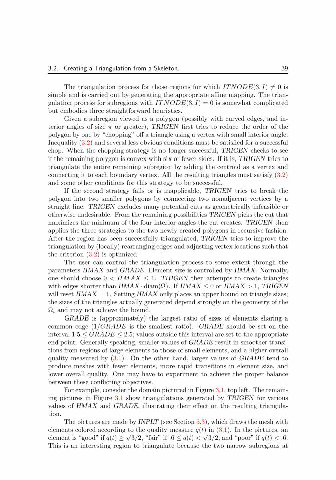
3.2. Creating a Triangulation from a Skeleton. 39
The triangulation process for those regions for which ITNODE(3, I) 6= 0 issimple and is carried out by generating the appropriate affine mapping. The trian-gulation process for subregions with ITNODE(3, I) = 0 is somewhat complicatedbut embodies three straightforward heuristics.
Given a subregion viewed as a polygon (possibly with curved edges, and in-terior angles of size π or greater), TRIGEN first tries to reduce the order of thepolygon by one by “chopping” off a triangle using a vertex with small interior angle.Inequality (3.2) and several less obvious conditions must be satisfied for a successfulchop. When the chopping strategy is no longer successful, TRIGEN checks to seeif the remaining polygon is convex with six or fewer sides. If it is, TRIGEN tries totriangulate the entire remaining subregion by adding the centroid as a vertex andconnecting it to each boundary vertex. All the resulting triangles must satisfy (3.2)and some other conditions for this strategy to be successful.
If the second strategy fails or is inapplicable, TRIGEN tries to break thepolygon into two smaller polygons by connecting two nonadjacent vertices by astraight line. TRIGEN excludes many potential cuts as geometrically infeasible orotherwise undesirable. From the remaining possibilities TRIGEN picks the cut thatmaximizes the minimum of the four interior angles the cut creates. TRIGEN thenapplies the three strategies to the two newly created polygons in recursive fashion.After the region has been successfully triangulated, TRIGEN tries to improve thetriangulation by (locally) rearranging edges and adjusting vertex locations such thatthe criterion (3.2) is optimized.
The user can control the triangulation process to some extent through theparameters HMAX and GRADE. Element size is controlled by HMAX . Normally,one should choose 0 < HMAX ≤ 1. TRIGEN then attempts to create triangleswith edges shorter than HMAX · diam(Ω). If HMAX ≤ 0 or HMAX > 1, TRIGENwill reset HMAX = 1. Setting HMAX only places an upper bound on triangle sizes;the sizes of the triangles actually generated depend strongly on the geometry of theΩi and may not achieve the bound.
GRADE is (approximately) the largest ratio of sizes of elements sharing acommon edge (1/GRADE is the smallest ratio). GRADE should be set on theinterval 1.5 ≤ GRADE ≤ 2.5; values outside this interval are set to the appropriateend point. Generally speaking, smaller values of GRADE result in smoother transi-tions from regions of large elements to those of small elements, and a higher overallquality measured by (3.1). On the other hand, larger values of GRADE tend toproduce meshes with fewer elements, more rapid transitions in element size, andlower overall quality. One may have to experiment to achieve the proper balancebetween these conflicting objectives.
For example, consider the domain pictured in Figure 3.1, top left. The remain-ing pictures in Figure 3.1 show triangulations generated by TRIGEN for variousvalues of HMAX and GRADE, illustrating their effect on the resulting triangula-tion.
The pictures are made by INPLT (see Section 5.3), which draws the mesh withelements colored according to the quality measure q(t) in (3.1). In the pictures, anelement is “good” if q(t) ≥
√3/2, “fair” if .6 ≤ q(t) <
√3/2, and “poor” if q(t) < .6.
This is an interesting region to triangulate because the two narrow subregions at

40 PLTMG USERS’ GUIDE 13.0
A skeleton with NTF = 6, NVF = 30, NBF = 35 (left). The triangulation for HMAX = 0,GRADE = 1.5 has NTF = 509, NVF = 292 (right).
The triangulation for HMAX = 0, GRADE = 2.0 has NTF = 329, NVF = 199 (left). Thetriangulation for HMAX = 0, GRADE = 2.5 has NTF = 262, NVF = 163 (right).
The triangulation for HMAX = .03, GRADE = 1.5 has NTF = 1269, NVF = 695 (left).The triangulation for HMAX = .06, GRADE = 1.5 has NTF = 634, NVF = 361 (right).
The triangulation for HMAX = .03, GRADE = 2.5 has NTF = 849, NVF = 480 (left).The triangulation for HMAX = .06, GRADE = 2.5 has NTF = 377, NVF = 227 (right).
Figure 3.1.

3.3. A Posteriori Error Estimates. 41
the top require small elements. TRIGEN tries to use larger elements in the largersubregions, but is constrained by the choices of HMAX and GRADE. DecreasingHMAX or GRADE tends to improve the overall quality of the triangulation, at theexpense of introducing more elements.
3.3 A Posteriori Error Estimates.Of central importance to the adaptive procedures is the computation of a posteriorilocal error estimates [2, 1, 64, 66]. In the case of piecewise polynomials of degreep, our a posteriori error estimate is based on a superconvergent approximation ofthe derivatives of u of order p [36, 37, 38]. In particular, given the finite elementfunction uh, we compute the piecewise linear vector functions Smh Qh∂
kx∂
p−ky uh, for
0 ≤ k ≤ p. where Qh is the L2 projection from the space of discontinuous piecewiseconstant functions into the space of continuous piecewise linear polynomials, andSh is a smoothing operator based on the discrete Laplace operator; in PLTMG, wetake m ≤ 1. See [36, 37, 38] for details. For meshes with variable p, we recoverderivatives patchwise, processing all elements of the same degree in the same patch.
The switch IERRSW allows the user to control the continuity of the recoveredderivatives. The options are specified in 3.2. In some problems, one expects thegradient or higher derivatives of the solution to be discontinuous, typically due todiscontinuities in the coefficient functions. If IERRSW = 1, a patchwise continuousrecovery is made. The user defines the patch boundaries by specifying differentvalues of ITNODE(5,*) for different patches. The parameter NDL is the combinedorder of the (block diagonal) linear systems that are used in the recovery.
IERRSW error recovery option
0 globally continuous recovery1 patchwise continuous recovery
Table 3.2. Patches are defined using element labels ITNODE(5,*).
Using these recovered derivatives, we compute a local error estimate εt fort ∈ T . Suppose the finite element space consists of continuous piecewise polynomialsof degree p, and denote by up the usual Lagrange interpolant. In [40], it is shownthat in many cases interpolation error is both an upper and lower bound on thefinite element error,
C1||∇(u− up)||L2(Ω) ≤ ||∇(u− uh)||L2(Ω) ≤ C2||∇(u− up)||L2(Ω),
implying that error indicators based on interpolation error are both reliable andefficient. In [27], constants involved in such estimates are numerically computedfor a variety of finite element spaces, including the Lagrange family of triangularelements used in PLTMG.
Our estimate is motivated by noting that under certain circumstances, ||∇(up+1−up)||L2(Ω) is an asymptotically exact estimate of ||∇(u − uh)||L2(Ω). This is known

42 PLTMG USERS’ GUIDE 13.0
for the cases p = 1 and p = 2 [37, 38]. Since the usual interpolation points forup and generally not a subset of those for up+1, on each individual element t, wereplace up+1 by up+1 = up + ep+1, where ep+1 is a locally defined polynomial ofdegree p + 1 that is zero at the interpolation points for the polynomial of degreep and has the same (constant) derivatives of order p + 1 as up+1 (see Figure 1.1).Such polynomials form a (local) vector space of dimension p+ 2. For example, e2 isa locally defined quadratic polynomial with value zero at all vertices of the mesh.On a given element t, e2 can be expressed as a linear combination of three quadratic“bump functions” qk associated with the edge midpoints of t,
e2 =
3∑k=1
`2kttkMttk qk(x, y) (3.3)
where `k is the length of edge k, tk is the unit tangent, and
Mt = −1
2
(∂xxu2 ∂xyu2
∂yxu2 ∂yyu2
).
is the Hessian matrix. All terms on the right hand side of (3.3) are known exceptfor the second derivatives appearing in the Hessian matrix Mt. In our local errorindicator, we simply approximate the second derivatives in the Hessian matrix Mt
using derivatives of SmQh∇uh. In particular, let
Mt = −1
2
(∂xS
mQh∂xuh ∂xSmQh∂yuh
∂ySmQh∂xuh ∂yS
mQh∂yuh
),
Mt =αt2
(Mt + M tt ), (3.4)
εt =
3∑k=1
`2kttkMttk qk(x, y).
The normalization constant αt is chosen such that the local error indicator ηt sat-isfies
ηt ≡ ||∇εt||L2(t) = ||(I − SmQh)∇uh||L2(t).
Normally we expect that αt ≈ 1, which is likely to be the case in regions wherethe Hessian matrix for the true solution is well defined. Near singularities, u isnot smooth and we anticipate difficulties in estimating the Hessian. For elementsnear such singularities, αt provides a heuristic for partly compensating for poorapproximation. For the cases ep+1, p > 1, more complicated formulas of similarnature are used. In particular, εt is expressed in terms of parameters describingthe geometry of t, and the derivatives of order p + 1 in t, that are obtained from∂xS
mh Qh∂
kx∂
p−ky uh, and ∂yS
mh Qh∂
kx∂
p−ky uh, for 0 ≤ k ≤ p, in a fashion analogous
to the case p = 1 described above. Global a posteriori estimates ||εt||L2(Ω) and||∇εt||L2(Ω) are stored as the parameters ENORM2 and ENORM1, respectively.
In the case of parameter identification problems, the error in the Lagrangemultiplier εt is computed by the a similar procedure to that described above. The

3.4. Adaptive Mesh Refinement and Unrefinement. 43
local error indicator is given by
ηt =||∇εt||2L2(t) + ||∇εt||2L2(t)
1/2
.
In the case of optimal control problems, errors in both the Lagrange multiplier εtand the control εt are computed, and the local error indicator is given by
ηt =||∇εt||2L2(t) + ||∇εt||2L2(t) + ||∇εt||2L2(t)
1/2
.
In both the cases, the definitions of ENORM1 and ENORM2 are similarly modified.Local error estimates are stored in the array E. This array has MAXT rows
and two columns. Row I of E corresponds to element tI , with entry E(I,1) = η2tI ,
and E(I,2) = αtI . The contents of the E array can be graphically displayed usingTRIPLT (see Section 5.2). The E array is typically updated in TRIGEN as part ofadaptive algorithms that make use of the error estimates. Thus if one is interestedin viewing uncorrupted versions of these quantities, plot them after calling TRIGENwith IADAPT = 0.
3.4 Adaptive Mesh Refinement and Unrefinement.Our adaptive algorithms are based on work described in Nguyen [57], Bank andNguyen [22, 24, 23, 25], Bank and Deotte [12], and Bank and Yserentant [41].When IADAPT = 1, the current mesh is adaptively refined or unrefined. When thetarget value NDTRGT > NDF, the mesh is refined, while if NDTRGT < NDF,the mesh is unrefined. In either case, the goal is to achieve the best possible meshusing (approximately) NDTRGT degrees of freedom. The switch IRTYPE specifiesthe type of adaptivity to be used – h, p, or hp as indicated in Table 3.3.
IRTYPE adaptivity option
0 hp refinement / unrefinement1 h refinement / unrefinement-1 p refinement / unrefinement
Table 3.3. Adaptivity options using IRTYPE.
When IADAPT = 2, both refinement and unrefinement are employed. First,the mesh is unrefined to obtained a mesh with approximately NDTRGT < NDFdegrees of freedom. The mesh is then refined to obtain a mesh with approximatelyNDF degrees of freedom. The output triangulation thus has approximately thesame number of degrees of freedom as the input triangulation, but the topology ofthe mesh and the distribution of degrees of freedom can be quite different.

44 PLTMG USERS’ GUIDE 13.0
3.4.1 Procedure Refine
Our hp refinement procedure is summarized in Figure 3.2. We initialize a heap datastructure where all elements are placed in the heap according to the size of ηt, withthe element with largest error indicator at the root.
Procedure Refine
R1 Create a heap with respect to ηt with thelargest error estimate ηtmax at the root;
R2 If NDF ≈ NDTRGT0, then go to R6.If η2
tmax ≤ η2ave/3, then go to R6.
R3 Execute case specific tests for h, p, and hprefinement of element tmax.
R4 Refine element tmax, and possibly others as required.R5 Update error indicators for affected elements.
Add new elements as needed. Remake the heap.Go to R2.
R6 Smooth the mesh based on geometry ((3.1)–(3.2)).Clean up data structures as needed.
Figure 3.2.
When IADAPT = ±1 and NDTRGT > NDF, the target number of degreesof freedom for the new mesh, denoted by NDTRGT0, is given by
NDTRGT0 = min(NDTRGT,NDF × 4). (3.5)
The use of (3.5) tries to force a geometric increase in the number of degrees offreedom in each refinement step. For the the case IADAPT = ±2, NDTRGT0 =NDF0, where NDF0 was the value of NDF when TRIGEN was entered.
While we normally expect the refinement loop to exit when the target numberof degrees of freedom is approximately achieved in line R2 of Procedure Refine,we can also exit if the largest error in the current mesh is sufficiently small. Inparticular,
η2ave =
1
N
∑t∈ΩI
η2t ≡ EAVE2, (3.6)
where ΩI is the fine subregion associated with processor I in the case of parallelcomputation, and ΩI ≡ Ω otherwise; N is the number of triangles in ΩI .
For hp-refinement, the critical test is to decide between between h-refinementand p-refinement for element tmax. The main test is to use h-refinement if
E(tmax, 2) ≡ αtmax ≥ 2. (3.7)
If the scaling factor αt ≈ 1, then the recovered derivatives and the error estimateare consistent, and we assume that the solution is locally smooth, which in turnjustifies p-refinement. Large values of αt empirically correspond to locally non-smooth behavior of the solution, and this in turn suggests h-refinement. See [25, 12]

3.4. Adaptive Mesh Refinement and Unrefinement. 45
for more detailed explanations and numerical experiments, and Bank, Parsania andSauter [28] for some convergence analysis.
While (3.7) is the main test for hp-refinement, we also make some case specifictests on line R3 of Procedure Refine. In the case of h-refinement, we test forpotential round-off error problems if h-refined elements become too small in size.In the case of p-refinement, we check to be sure the p-refined element will havedegree less than MXORD. We require that MXORD ≤ 9 due to limits on the orderof accuracy for the suite of numerical quadrature rules implemented in PLTMG.These quadrature formulas were provided by Zhang, Cui, and Liu in [67]. Failureof these case specific tests could reverse the decision suggested by (3.7). Finally, ifelement tmax has degree k, and
RELERP ≤ 1
5× 3k−1(3.8)
then h-refinement is selected. The thresholds (3.8) are based on the empiricalobservation that it is efficient to require sufficiently many elements in the mesh (asmeasured by (3.8)) before allowing increasingly higher degree elements.
At the conclusion of the main refinement loop, in R6 we smooth the mesh,locally “flipping” edges and adjusting the location of vertices to locally optimizethe geometric quality measure q(t) given in (3.1).5
3.4.2 Procedure Unrefine
Our unrefinement procedure is complementary to the refinement procedure, as sum-marized Figure 3.3. In many details, it implements the opposite rules of ProcedureRefine. For example, we initialize a heap data structure where all elements areplaced in the heap according to the size of ηt, but now with the element tmin withthe smallest error error indicator at the root.
If IADAPT = ±1 or IADAPT = ±2, then NDTRGT0 is given by
NDTRGT0 = max(NDTRGT,NDF/4).
This generally provides a geometric decrease in the number of degrees of freedom.The parameter ηave in U2 is computed as in (3.7).
For hp-unrefinement, the main test is based on (3.7). If (3.7) and
RELERP ≥ 1
5
are both satisfied, then use h-unrefinement; otherwise use p-unrefinement. Our biashere is to try to preserve the largest number of elements in the mesh. The resultof this test is possibly changed on the basis of the h and p specific tests mentionedbelow. The case specific test for h-unrefinement determines the best vertex of
5In adjusting the mesh, we take into account constraints imposed by boundary geometry,boundary conditions, and internal interfaces defined by the the user or by PLTMG in the contextof parallel computation.

46 PLTMG USERS’ GUIDE 13.0
Procedure Unrefine
U1 Create a heap with respect to ηt with thesmallest error estimate ηtmin at the root;
U2 If NDF ≈ NDTRGT0, then go to U6.If η2
tmin ≥ η2ave/2, then go to U6.
U3 Execute case specific tests for h or punrefinement of element tmin.
U4 Unrefine element tmin, and possibly others as required.U5 Update error indicators for affected elements.
Remove elements as needed. Remake the heap.Go to U2.
U6 Smooth the mesh based on geometry ((3.1)–(3.2)).Clean up data structures.
Figure 3.3.
element tmin to be removed from the mesh.6 For p-unrefinement, an element musthave degree at least two.
Similar to Procedure Refine, at the conclusion of Procedure Unrefine, the finalmesh is smoothed, and some edges possibly flipped in U6 to locally optimize thegeometric quality as measured by (3.1).
3.4.3 h Refinement
Our basic h-refinement algorithm uses a relaxed version of the longest edge bisectionprocedure of Rivara [52, 61] but does not generate a refined element tree. Theelement tmax to be refined is bisected along it longest edge. If tmax has a neighborelement across its longest edge, and the shared edge is longer than 0.9 times itslongest edge, then it is refined. If not, the neighbor is refined along its longestedge, and the procedure described above is recursively applied to its longest-edgeneighbor. An example is shown is Figure 3.4. The classic (unrelaxed) longestedge bisection process is known to have finite termination, typically in a very smallnumber of steps. The relaxation factor 0.9 attempts to make the process terminateeven sooner; it is small enough that the test is satisfied by most shape regularelements, so that only one edge is bisected in most steps of R4 in Procedure Refine(Figure 3.2).7
When our relaxed longest edge bisection process finally results in a triangu-lation, elements are bisected, new elements created, (in reverse order to alwaysmaintain a triangulation) and the triangulation data structures updated. New el-ements inherit the (constant) derivative values from their parents, allowing errorestimates to be computed for the refined elements, and the heap to be updated.
6Certain vertices lying on the boundary or on internal interfaces are not eligible to be removedfrom the mesh. In exceptional cases an element might be deemed ineligible for h-unrefinement.
7Since shape regularity is improved in step R6 of Procedure Refine, we relax shape regularityrequirements during the refinement process itself to improve efficiency.

3.4. Adaptive Mesh Refinement and Unrefinement. 47
@@
@@@
@@@@@
t
@@
@@@
@@@@@
@@
@@@
@@@@@
Figure 3.4. Element t is refined by the longest edge bisection method.The original mesh is on the left. The first step of bisection (middle) does not yielda compatible triangulation. However, the second step (right) does yield a triangula-tion.
3.4.4 h Unrefinement
In the case of h-unrefinement, the basic step consists of deleting vertices from themesh; this is accomplished by merging two vertices of element tmin that share acommon edge. This is illustrated in Figure 3.5.
@@
@@
@
@@@@@
−→ ←−t
v v′
Figure 3.5. Element t is unrefined by the merging vertices v and v′, andcollapsing the edge connecting them. The location of the merged vertex could be v,v′, or (v + v′)/2, depending on the shape quality of other elements having v or v′
as one of their vertices.
While this merging process tends to degrade the geometric quality of sur-rounding elements, it is typically restored in step U6 of Procedure Unrefine, whenelement edges are flipped and vertices moved to locally optimize the quality measure(3.1).
48 PLTMG USERS’ GUIDE 13.0
3.4.5 p Refinement
The p-refinement algorithm is relatively straightforward. Let element tmax havedegree p with edges of degree pi ≥ p, 1 ≤ i ≤ 3. The refined element has degreep + 1 with edges of degree maxpi, p + 1, 1 ≤ i ≤ 3. As a technical point, sincewe require degrees of freedom associated with element interiors and edges haveconsecutive global indices,8 storage arrays (e.g., GF) have degrees of freedom forp-refined edges and interiors appended to their tails, leaving gaps where earlier edgeand interiors degrees of freedom were stored. There is a global cleanup step at theend of the refinement process to compress the data structure and remove these gaps,similar to that performed at the end of unrefinement algorithms.
3.4.6 p Unrefinement
p-unrefinement is similar in structure to p-refinement. An element of degree p hasit interior decreased to degree p− 1. The edge degrees of freedom pi, 1 ≤ i ≤ 3, arereduced to pi − 1 or remain at degree pi, depending on the degree of the neighborelement (if present) that shares the given edge. In the case of degree reduction, thereduced degrees of freedom can occupy space previously used by the higher degreeedges or interior degrees of freedom, leaving small gaps in these data structures thatare removed at the end of the unrefinement process.
3.5 Adaptive Mesh Smoothing.When IADAPT = ±3, subroutine TRIGEN does no refinement or unrefinementof the mesh but rather adjusts the (x, y) coordinates of the mesh points (VX andVY ) in an attempt to optimize the mesh.
The procedure consists of a Gauss–Seidel-like iteration on the vertices in themesh, where each vertex is locally optimized with all other vertices held fixed [31].Four sweeps are performed in each call. Let Ωv denote the patch of elements thatshare a given vertex v; an example is shown in Figure 3.6. Typically, vertex vis allowed to move within the region Ωv. However, not all vertices in the meshare allowed to move. Some boundary and interface vertices must remain fixed topreserve the definition of the region. These vertices are called corners. Cornersinclude actual geometric corners of the region, vertices where boundary conditionschange type or label, vertices where interfaces intersect the boundary, and verticeswhere two or more interfaces intersect. An interface here is taken as any sequenceof triangle edges that separate triangles with different user defined labels. Verticeson the boundary or on interfaces that are not designated corners are allowed tomove only along the boundary or interface. The remaining vertices, called interiorvertices, are allowed to move freely within Ωv. As in our refinement algorithms,some local mesh smoothing based on (3.1) is used to locally optimize the shaperegularity of the mesh.
8Having consecutive indices for interior and edge degrees of freedom makes the amount ofinformation stored in array ITDOF for a given element independent of its degree.

3.6. Uniform Refinement. 49
v
Figure 3.6. Subregion Ωv is associated with vertex v.
For each vertex v = (x, y) in the mesh, we solve the minimization problem
minx,y||∇εt||2L2(Ωv) (3.9)
of order two by a damped Newton’s method. As noted above, we assume thederivatives of order p+1 are constant in each element t having v as a vertex, leadingto an overall piecewise constant approximation of these derivatives on Ωv. All otherdependencies on v = (x, y) are taken into account by Newton’s method. Boundaryand interface vertices have an additional constraint equation, so an appropriatelyconstrained version of problem (3.9) is solved for those vertices. Besides its usualtask of ensuring sufficient decrease, the damping strategy for Newton’s method isalso used to ensure that the point (x, y) remains well within Ωv, so that all trianglesare always well defined. It is interesting to note that the function ||∇εt||L2(Ωv)
contains a natural barrier function that becomes infinite as (x, y) approaches ∂Ωv.In the case IADAPT = −3, the adaptive smoothing procedure uses the inter-
polation errors for the function QXY in place of the a posteriori error estimates, ina fashion analogous to the cases of refinement and unrefinement with IADAPT < 0.
3.6 Uniform Refinement.TRIGEN allows options for uniform refinement in h and p. In the standard sequen-tial setting, the uniform refinement is standard and straightforward. In the case ofparallel computation, each processor approximately uniformly refines its own sub-region. If the parallel computation uses NPROC processors, each processor addsapproximately 1/NPROC of the expected increase in degrees of freedom resultingfrom uniform refinement in the standard sequential case. Because different subre-gions can have widely varying numbers of elements, this can result in different levelsof uniform refinement in different regions. See Section 3.8 for discussion of the meshpartitioning process.

50 PLTMG USERS’ GUIDE 13.0
3.6.1 h Uniform Refinement
When IADAPT = 4, subroutine TRIGEN performs uniform h-refinement of theexisting triangulation. The refinement is controlled by the parameter IREFN >1. Each element in the triangulation is uniformly divided into IREFN2 similartriangles. Some examples are shown in Figure 3.7. If IADAPT = 4 and MPISW =1, the situation is different. In this case, TRIGEN tries to increase the globaldimension of the space by roughly a factor of IREFN2. The target value for eachprocessor is given by
NDTRGT0 = min
(NDTRGT,NDF ×
1 +
IREFN2 − 1
NPROC
).
Each processor refines uniformly, restricting this refinement mainly to region IRGN.Rather than the uniform refinement described above, the relaxed longest edge pro-cedure is used. Regions with relatively few elements may require several levels ofrefinement to achieve the target number of degrees of freedom; those with manyelements may need only one partial level of refinement to achieve this target. In thecase of partial levels of refinement, the elements chosen to be refined are essentiallyrandom.
Figure 3.7. Uniform refinement for the cases IREFN = 2, 3, 4.
3.6.2 p Uniform Refinement
When IADAPT = −4, subroutine TRIGEN performs uniform p-refinement of theexisting triangulation. The refinement is controlled by the parameter IREFN >0. In this case, every element interior of degree p is increased to degree min(p +IREFN ,MXORD), and every edge of degree pi is increased to degree min(pi +IREFN ,MXORD). If IADAPT = −4 and MPISW = 1, TRIGEN does uniform prefinement, but restricts this refinement mainly to region IRGN. In this case, thetarget number of degrees of freedom is given by
NDTRGT0 = min
(NDTRGT,NDF ×
1 +
[(pave + IREFN)/pave]2 − 1
NPROC
),

3.7. An Example 51
where pave estimates the average degree of elements in the mesh and is given by
pave =
√NDF
NVF.
Similar to the case of IADAPT = 4, degrees of some elements may be increased bymore than IREFN if few elements are present in IRGN. If there are many elementsin IRGN some elements may have their degrees increased by less than IREFN, oreven left unchanged. The elements chosen for partial levels of p refinement areessentially random, as in the case of h uniform refinement.
3.7 An ExampleSome examples of our adaptive procedures are shown in Figures 3.8–3.9. In theseexamples, we employ the alternate function QXY = r1/4 sin(θ/4) defined on thecircular domain with a crack shown in Figure 2.1. The initial mesh with NVF = 10is shown in Figure 3.8, top. The mesh was then refined with IADAPT = −1 toproduce a sequence of hp adapted meshes. In Figure 3.8, we see the resulting meshwith NTF = 9824 elements and NDF = 43319 degrees of freedom.
In the next experiment, we begin with the same mesh with NTF = 8 elementsand uniformly refine it using IADAPT = 4 and IREFN = 8, creating a uniformmesh of NTF = 512 elements. We the uniformly refine in p (IADAPT = −4 andIREFN = 2) to create a uniform mesh of piecewise cubic polynomials with a totalof NDF = 2425 degrees of freedom.
We employ adaptive mesh smoothing (IADAPT = −3); in Figure 3.9 we seethe results of one step and eight steps of mesh smoothing. It is visually apparentthat the mesh smoothing tries to concentrate degrees of freedom near the singularityat the origin. However, mesh smoothing is limited by the constraint that the meshtopology remain invariant, and this ultimately limits its effectiveness in this setting.
Next, we call TRIGEN int IADAPT = −2 (unrefine and refine) and NVTRGT =1800. The results are shown in Figure 3.9, where the mesh is colored by both poly-nomial degree and by element size. We see that in the unrefinement phase, mostof the coarsening consisted mostly of p-unrefinement, reducing the polynomial de-gree from three to two in those elements most distant from the origin, when theerror should be smallest. The refinement step was mostly h-refinement, where el-ements near the origin were refined. This seems like a reasonable outcome giventhat the unrefinement and refinement steps are conducted sequentially and indepen-dently. However, one could argue that a more informed strategy in this situation isto coarsen in p the elements near the origin, which have larger errors, and then h-refine those elements using lower degree polynomials. Such a strategy requires morespecialized coarsening and refinement algorithms than currently exist in PLTMGand is a topic for future research.
3.8 Parallel Adaptive Methods.In this section we summarize the general strategy for adaptive mesh generationthat is implemented in PLTMG. A number of static and dynamic load balancing

52 PLTMG USERS’ GUIDE 13.0
The initial triangulation with NTF = 8, NVF = 10, and NBF = 10.
The refined triangulation with NTF = 9824, NDF = 43319. Elements are colored bypolynomial degree (left) and by element size (right).
The refined triangulation with NTF = 9824, NDF = 43319. The mesh is magnified nearthe origin with RMAG = 1016, revealing the presence of low degree polynomials (left) andvery small elements (right).
Figure 3.8.
approaches for unstructured meshes have been proposed in the literature [65, 62,45, 48, 42, 50, 43]; most of the dynamic strategies involve repeated application ofa particular static strategy. One of the difficulties in all of these approaches is theamount of communication that must be performed both to assess the current loadimbalance severity, and to redistribute the work among the processors once theimbalance is detected and an improved distribution is calculated.
The approach used by PLTMG is based upon the Bank-Holst paradigm [15,16, 4, 26, 58, 53, 54], that addresses the load balancing problem in a new way,requiring far less communication. Another important point is that our approach

3.8. Parallel Adaptive Methods. 53
A uniformly refined mesh with NTF = 512, NVF = 297, and NBF = 80.
The uniformly refined mesh after one step of mesh smoothing (IADAPT = −3), withpiecewise cubic elements, NDF = 2425 (left). The same mesh after eight steps of meshsmoothing (right).
The mesh resulting from one step of unrefinement and refinement (IADAPT = −2) withNDTRGT = 1800. The resulting mesh is colored by polynomial degree (left) and elementsize (right) and has NTF = 647 elements with NDF = 2422 degrees of freedom.
Figure 3.9.
allows PLTMG to run in a parallel environment without a large investment inadditional coding. This approach has three main components:
Step 1: A small (nonlinear) problem is solved on an initial coarse mesh, and a pos-teriori error estimates are computed for the coarse grid solution. The tri-angulation is partitioned such that each subdomain has approximately equalerror (although they can significantly differ in size, numbers of elements anddegrees of freedom).

54 PLTMG USERS’ GUIDE 13.0
Step 2: Each processor is provided the complete coarse mesh and solution, and in-structed to solve the entire (nonlinear) problem, with the stipulation that itsadaptive refinement should be limited largely to its own partition. Load bal-ancing is achieved by instructing each processor to create a refined mesh withthe same number of degrees of freedom.
Step 3: A final mesh is computed using the union of the refined partitions provided byeach processor. This mesh is reconciled such that the (virtual) mesh made upof the union of the refined subregions would be conforming. A final solution iscomputed, using a domain decomposition method. An initial guess is providedby the local solutions.
The above approach has several interesting features. First, the load balancingproblem (Step 1) is reduced to the numerical solution of a small problem on a singleprocessor, without requiring any modifications to PLTMG. Second, the adaptivemesh generation calculation (Step 2) takes place independently on each processor,and can also be performed with no communication.
The only parts of the calculation requiring communication are
1. the initial fan-out of the mesh distribution to the processors, once the decom-position is determined by the error estimator.
2. the mesh regularization, requiring communication to produce a global con-forming mesh.
3. the final solution phase. Note that a good initial guess for Step 3 is providedin Step 2 by taking the solution from each subregion restricted to its partition.
The options 6 ≤ IADAPT ≤ 7 provide basic parallel mesh management toolsthat support this paradigm. The domain decomposition solver is implemented as anoption in subroutine PLTMG. These options require the use of MPI library routinesfor communication.
The basic strategy employed in Step 2 is an adaptive feedback loop
solve→ estimate→ refine.
The solve phase of this loop is realized by subroutine PLTMG while the estimate andrefine phases are realized by subroutine TRIGEN. A potential problem arises fromthe possibility that with hp refinement, it is highly likely that different processorswill require different numbers of feedback loops in order the achieve a given targetnumber of degrees of freedom. See [12, 41] for some discussion of this topic. Evenin the simple case of h refinement, it might be difficult to estimate the number offeedback loops that might be needed to achieve the target number of degrees of free-dom. The parameter NOCHNG addresses this issue by providing a communicationlink between subroutines PLTMG and TRIGEN as summarized in Table 3.4.
A normal call to TRIGEN will return with NOCHNG = 0. However, ifTRIGEN determines that the target number of degrees of freedom has alreadybeen achieved, it sets NOCHNG = 1 and returns with no further computation.

3.8. Parallel Adaptive Methods. 55
NOCHNG refinement option
0 normal call to TRIGEN1 target degrees of freedom achieved
Table 3.4. The parameter NOCHNG.
If PLTMG is called with NOCHNG = 0, it will proceed normally. If PLTMG iscalled with NOCHNG = 1, it will return without further computation, since thesubspace was unchanged by the previous call to TRIGEN. This allows the user toprovide an overestimate the number of feedback loops required without incurringthe penalty of additional computational costs. In this scenario, all processors canachieve NDTRGT degrees of freedom, although each may require a different numberof feedback loops to do so.
3.8.1 Mesh Partitioning.
When IADAPT = 6, TRIGEN computes a posteriori error estimates and partitionsthe mesh as in the Bank-Holst paradigm. If PLTMG is running on NPROC proces-sors, then the mesh is partitioned into NPROC subregions, such that each subregionhas approximately equal error. Deotte [46] and Bank and Deotte [13] examine sev-eral partitioning strategies, including the one used in PLTMG, and in particularstudy their effect on the convergence rate of Domain Decomposition solvers usingsuch partitions. The underlying algorithm employed is a variant of the recursivespectral bisection algorithm [44, 60, 63]. While this particular mesh partitioningalgorithm is among the more expensive of the choices that we could make, it istypically used only once on a relatively small problem. Although this calculation isimportant in the parallel processing environment, it is done on a single processorand does not use the MPI library. At the conclusion of the load balancing step,TRIGEN creates new internal edges in IBNDRY at the interface between differentsubregions. Then the processor corresponding to IRGN = 1 broadcasts its mesh,solution, and supporting data to all processors using an MPI broadcast command.
The partitioning process begins with the creation of patches of elements withsmall errors called macro-elements. Macro-element patches contain a minimum ofone and a maximum of 100 elements and must form a geometrically connected set.Let
E =1
NPROC
∑t
||∇εt||2L2(t).
For a patch P , let
EP =∑t∈P||∇εt||2L2(t).
If the patch P contains more than one element, we require EP ≤ 10−2 × E.Suppose the mesh is composed of N macro-elements. We define the N × N

56 PLTMG USERS’ GUIDE 13.0
symmetric, positive semi-definite M -matrix A by
Aij =
−` i 6= j and patches i and j share ` common edges
0 i 6= j and patches i and j share no common edgesi i = j, si = −
∑k 6=iAik
Macro element patches are created to reduce the order of the matrix A, and thusreduce the cost of solving the eigenvalue problems described below. The matrixA corresponds to the discrete Laplacian for the dual graph of the macro elementmesh, in which the macro elements are considered nodes, and the off-diagonal entriescorrespond to edges defined by the adjacency relation, weighted by the number ofoverlapping edges in the original triangulation.
We consider the eigenvalue problem
Aψ = λψ (3.10)
Our approach is standard; by construction, the smallest eigenvalue for (3.10)is λ1 = 0 and ψ1 = (1, 1, . . . , 1)t. Our interest is in the second eigenvector ψ2,known as the Fiedler vector.
We use a standard binary tree with 2NPROC − 1 nodes (NPROC leaves andNPROC − 1 internal nodes). The root is labeled i = 1 and node i has children2i and 2i + 1, 1 ≤ i ≤ NPROC − 1. Associated with each node is a weight ωidenoting the number of leaves contained in its subtree. In particular, ωi = 1,i = 2NPROC − 1, . . . ,NPROC and ωi = ω2i + ω2i+1 for i = NPROC − 1, . . . , 1.
The entire mesh is assigned to root, and it is partitioned among its two childrenas follows. We first approximately solve the eigenvalue problem (3.10) for the wholemesh, and then create a permutation of the macro-elements qi such that
qi < qj implies ψ2,i ≤ ψ2,j .
We then find the index k which provides the best partition of the form
1
ω2
∑qi≤k
EPqi ≈1
ω3
∑qi>k
EPqi .
The corresponding submeshes are assigned to the children nodes.We apply this procedure recursively, at each level dividing each group of ele-
ment patches into two smaller groups by solving an eigenvalue problem of the type(3.10) restricted to that group of patches. The final result is NPROC subregionswith approximately equal error E.
We now briefly describe some details of our procedure for computing the sec-ond eigenvector of (3.10). Our procedure is essentially just a classical Rayleighquotient iteration [59], modified both to bias convergence to λ2, and to account forthe fact that the linear systems arising in the inverse iteration substep are solved(approximately) by an iterative process. To simplify notation and avoid multiplesubscripts, we let φk ≈ ψ2, where k now denotes the iteration index.
We suppose that we have a current iterate φk which satisfies φtkφk = 1 and
ψt1φk = 0. Using φk, we compute the approximate eigenvalue λ2,k ≈ λ2 from the

3.8. Parallel Adaptive Methods. 57
Rayleigh quotient λ2,k = φtkAφk, and approximately solve the linear system
Aδk = rk ≡ λ2,kφk −Aφk.
Note that by construction ψt1rk = φtkrk = 0. This linear system is approximatelysolved using a simple Symmetric Gauss-Seidel iteration.
From δk, we form the vector δk satisfying δtkδk = 1 and ψt1δk = φtkδk = 0.
Finally, we solve the 3× 3 eigenvalue problem for A, where
A =
φtkδtkξtk
A(φk δk ξk
)where ξk is defined below. If v = (α, β, γ)t is an eigenvector corresponding to thesmallest nonzero eigenvalue, we form φk+1 = αφk+βδk+γξk and ξk+1 = βδk+γξkwith ξ1 = 0. Then φk+1 and ξk+1 are formed from φk+1 and ξk+1, respectively, bynormalization and orthogonalization to ψ1. Solving the 3 × 3 eigenvalue problemrather than a 2× 2 problem was motivated by the work of Knyazev [49].
3.8.2 Reconciling the Mesh.
The option IADAPT = 7 reconciles the mesh. This is the most complex of the MPIoptions in TRIGEN, and is typically called once, at the conclusion of the second stepof the Bank-Holst paradigm. It must be called before the domain decompositionsolution in subroutine PLTMG, as PLTMG makes use of the parallel interface datastructure IPATH generated by this call.
In creating the IPATH data structure, each processor first organizes its tri-angulation and solution data structures. Generally, edges, vertices, and degreesof freedom on the interface between region IRGN and the rest of the domain ap-pear first in their respective arrays (IBNDRY, VX, VY, GF, etc). This data isorganized to correspond to counter clockwise traversal of the interface. Next inall arrays comes data corresponding to the interior of subregion IRGN ; generally,this should be the majority of the data. Finally, at the end of each array appearsdata corresponding to regions other than IRGN. Each processor then assembles itscontributions to the preliminary IPATH array based on the reordered data, andthis information is then exchanged among processors using MPI (see Section 2.6).
After the boundary exchange, each processor tries to match its boundaryinterface edges to those provided by neighboring regions, in order to establish thestructure of the global mesh. Typically this mesh is not conforming. When non-matching edges are found, the region that is less refined does additional refinementuntil its boundary edges form a one-to-one match with those of its neighbors. Anexample is shown in Figure 3.10.
After the mesh is made h-conforming it is made p-conforming. When a p-nonconforming edge is found, the region containing the edge of lower degree p-refinesits edge appropriately in order to resolve the nonconformity.
Each processor then reorders its data structures and communicates its con-tribution to the IPATH array a second time. This time the edge matching process

58 PLTMG USERS’ GUIDE 13.0
JJJJJAAAAAAAA
AAAAAAAA@@@@
Ωi
Ωj
JJJJJAAAAAAAA
AAAAAAAA@@@@
Figure 3.10. The coarse side of a non matching interface (left) is refinedto make the global mesh conforming (right).
concludes with no nonconforming edges found. By matching boundary edges at theinterface, one also effectively matches degrees of freedom on the interface; it is thisinformation that is needed for the domain decomposition solver.

Chapter 4
Equation Solution
4.1 Overview.Subroutine PLTMG solves the problems described in Section 1.1. The solutionprocess for each class of problems has certain unique aspects, but all make use ofNewton’s method. Subroutine PLTMG is entered using the statement
Call PLTMG( VX, VY, SF, ITNODE, IBNDRY, ITDOF, IPATH,E, IP, RP, SP, GF, A1XY, A2XY, FXY, GNXY, GDXY,P1XY, P2XY, SXY )
On input, the arrays VX, VY, SF, ITNODE, ITDOF, and IBNDRY definea triangulation. Arrays IPATH E, and GF are discussed in Sections 2.5 and 2.6.Fortran subroutines A1XY, A2XY, FXY, GNXY, GDXY, P1XY, and P2XY aredocumented in Section 2.8. Subroutine SXY is documented in Section 2.2. Param-eters in the IP, RP, and SP arrays read and written by PLTMG are summarizedin Tables 2.12–2.14.
The parameter IPROB indicates the problem class; the various options areshown in Table 4.1. The case IPROB > 0 indicates a standard sequential solve,either on a single processor, or on multiple processors as part of the second phaseof the Bank-Holst paradigm. The case IPROB < 0 indicates the global paralleldomain decomposition solve as part of the Bank-Holst paradigm. Because this isa global solve it involves some MPI communication at each iteration step. WhenIPROB < 0, the parallel domain decomposition solve is preceded by a local solveon each processor, in order to insure the quality of the initial guess for the globalproblem.
The cases IPROB = ±3 and IPROB = ±4 have various suboptions uniqueto their particular problem class. The available options are specified through theparameter ITASK . These are summarized in Table 4.2.
59

60 PLTMG USERS’ GUIDE 13.0
IPROB problem option
1 elliptic boundary value problem2 obstacle problem3 continuation problem4 parameter identification problem5 optimal control problem
-1 DD solve for elliptic boundary value problem-2 DD solve for obstacle problem-3 DD solve for continuation problem-4 DD solve for parameter identification problem-5 DD solve for optimal control problem
Table 4.1. The parameter IPROB.
ITASK IPROB option
0 1 default9 use functional
0 2 default
0 continue to the nearest target point1 continue to the nearest target or singular point2 switch branches at a bifurcation point3 3 switch λ and/or ρ; initialize with λ fixed4 switch λ and/or ρ; initialize with ρ fixed5 solve with σ = 0, θ = 0 (λ fixed)6 solve with σ = 0, θ = 2 (ρ fixed)7 solve with σ = 0, θ = 1
0 4 default8 λ affects domain shape
0 5 default
Table 4.2. The parameter ITASK.
4.2 Elliptic Boundary Value Problems.When IPROB = 1, PLTMG solves the discrete system (1.6). If the underlyingboundary values problem is not self-adjoint some upwinding terms inspired by theScharfetter–Gummel discretization scheme [7, 11] are added to the discretization;in this case (1.6) should be replaced by: find uh ∈Md such that
ah(uh, v) = 0 for all v ∈Me, (4.1)

4.2. Elliptic Boundary Value Problems. 61
where ah(uh, v) reflects the additional stabilization terms. We note that the up-winding terms are derived for the case of piecewise linear finite elements (p = 1).While a similar upwinding scheme is also formally applied to higher degree elements,its stability and convergence properties are not yet analyzed. In any event, (4.1)corresponds to the system of nonlinear equations
G(U) = 0, (4.2)
where the unknown vector U corresponds to the values of the finite element solutionuh at the vertices of the triangulation. The Jacobian matrix
A(U) =∂G(U)
∂U
is a sparse stiffness matrix corresponding to a linear elliptic boundary value problem(linearized about U). Even in the event the the original problem is linear, PLTMGsolves all problems with IPROB = 1 as nonlinear, and formally applies Newton’smethod to (4.2). In Figure 4.1, we summarize our approximate Newton procedurewith line search.
Procedure Newton
N1 Begin with initial guess U0, and a sufficientdecrease parameter τ . Set k ← 0,s0 ← 1, and compute G0 and ||G0||.
N2 solve (approximately) AkδUk = −G(Uk).N3 compute Uk+1 = Uk + skδUk, Gk+1, ||Gk+1||, and
ξk+1 = ||Gk+1||/||Gk||.N4 if 1− ξk+1 < τsk, then decrease sk and go to N3;
else set sk+1 ← sk/(sk + (1− sk)ξk+1/100)and k ← k + 1.
N5 if converged, then exit; else go to N2.
Figure 4.1.
The scalar sk is the damping parameter. When the sufficient decrease crite-rion is not satisfied on line N4 and sk must be reduced, the next value is foundthrough application of one step of a guarded secant/bisection algorithm to the one-dimensional minimization problem
minsk||G(Uk + skδUk)||.
If sufficient decrease is achieved, the current sk is used to predict sk+1; this formula isdesigned to force rapid increase of sk+1 → 1 when ξk+1 becomes small as superlinearconvergence occurs, and at the same time provide a reasonable first guess in theearly stages of the Newton iteration, when damping is most important. A maximumof MXNWTT damped Newton iterations are allowed. PLTMG reports the actualnumber of Newton iterations used on the most recent call in the parameter ITNUM,

62 PLTMG USERS’ GUIDE 13.0
and the number of evaluations of G as IEVALS; IEV ALS ≥ ITNUM , since morethan one function evaluation may be used in each line search.
As a simple example, we solve the Poisson equation
−∆u = 1 in Ω,u = 0 on ∂Ω,
The domain Ω was provided as a skeleton and is shown in Figure 4.4. This problemwas solved using hp adaptive refinement using eight processors. The skeleton wastriangulated, and then a mesh with NVF = 1879 and NDF = 5358, was adaptivelycreated on one processor. The processor then did a load balance step (IADAPT =6 in TRIGEN) and broadcast this mesh to all processors. The load balance isshown in Figure 4.4. Each processor then independently continued the refinementprocess on its subregion, using a maximum of five hp adaptive refinement steps.The global refined mesh was made conforming (IADAPT = 7 in TRIGEN) and thedomain decomposition solver invoked in PLTMG (IPROB = −1). The resultingglobal mesh had NDF = 221657 degrees of freedom; the global solution is shownin Figure 4.4. The global mesh colored by element size and polynomial degree isshown in Figure 4.4, along with a timing summary for the entire calculation, and aconvergence history for the Domain Decomposition solver (see Section 4.4).
4.3 Linear Solvers.All sets of linear equations involving the matrices A(U) and A(U)t have the ap-pearance of finite element discretizations of linear elliptic boundary value problems.These systems can be solved using a variety of preconditioners, coupled with thecomposite step conjugate gradient method (ISPD = 1) or composite step biconju-gate gradient method (ISPD = 0). The composite step algorithms [10, 9] are similarto the standard biconjugate gradient and conjugate gradient methods, respectively,except that they occasionally proceed from the iterate for step k to the iterate forstep k+2. Such composite steps are taken to improve the stability of the recurrencerelations and smooth the behavior of the residual norm. Note in particular thatthe composite step conjugate gradient method can be applied to symmetric butindefinite problems. The maximum number of iterations to be used per solutionis specified by the parameter MXCG. Note that as many as MXCG iterations areused each time a system of linear equations is solved.
The selection of preconditioner is governed by the parameter METHOD assummarized in Table 4.3. Combinations of three different matrices are used in com-posing these preconditioners. We remark that in all cases the matrices are orderedusing a (block) minimum degree algorithm. In particular, dense blocks correspond-ing to element interior degrees of freedom are always ordered first, as these blockscould be eliminated through Gaussian Elimination (static condensation) withoutcausing any fill-in.
ILU is an incomplete LDU factorization based on the multigraph algorithm[33, 32]. The parameter DTOL is the drop tolerance for this approximate factoriza-tion. Generally, smaller values of DTOL result in more accurate ILU factorizations,

4.3. Linear Solvers. 63
The skeleton with NVF = 135 (left) and the resulting triangulation with NVF = 1381(right).
The mesh with NDF = 5358 showing the load balance (left), and the solution on the globalfine mesh NDG = 221657 (right).
The global refined mesh colored by element size (left) and by polynomial degree (right).
Some timing statistics (left) and convergence history for the DD solver (right).
Figure 4.2.

64 PLTMG USERS’ GUIDE 13.0
METHOD preconditioner
0 Block SGS smoother, HB coarse space1 ILU
Table 4.3. The parameter METHOD.
but higher costs in space and time per iteration. The extreme case DTOL = 0 re-sults in a sparse direct factorization.
SGS is a block symmetric Gauss-Seidel preconditioner, based on the diagonal,upper and lower triangular blocks of the matrix A. The diagonal blocks of A arefactored using dense LDU factorizations. HB is a coarse grid correction based onhierarchical basis. LetM denote the hp finite element space used in assembling thematrix A. Our coarse space Mc ⊂ M is composed as the union of the followingsets of basis functions.
1. A standard continuous piecewise linear nodal basis function is associated witheach vertex in the mesh.
2. For every edge in the triangulation with p ≥ 2, we associate a continuous piece-wise quadratic nodal basis function (quadratic bump function) correspondingto the edge midpoint.
3. For every element in the triangulation with p ≥ 3, we associate a continuouspiecewise cubic nodal basis function (cubic bubble function) corresponding tothe element barycenter.
The maximum dimension ofMc is approximately 6×NVF, if every quadratic bumpand cubic bubble function is present. The coarse space matrix Ac is computed fromA by
Ac = StAS
for an appropriately defined rectangular change of basis matrix S. Then we computean approximate LDU factorization of the matrix Ac. The parameter DTOL is thedrop tolerance for this approximate factorization. This approximate factorizationserves as the coarse grid correction in a two-level preconditioner. One cycle of thetwo level iteration consists of one pre-smoothing step (SGS), followed by the coarsegrid correction step, and one post-smoothing step (SGS). See [6] for additionaldiscussion.
As a general remark, the SGS/HB two-level solver typically requires less setuptime but more solution time compared to ILU. Overall, ILU becomes increasinglyeffective when there are many high degree elements and the matrix A becomesincreasingly dense. ILU also is very effective on convection dominated highly non-symmetric problems. The SGS/HB two-level solver is most effective when thereare many low degree elements in the mesh. Finally, note that a direct method isavailable using ILU with DTOL = 0.

4.4. Domain Decomposition Solver 65
4.4 Domain Decomposition SolverHere we describe the domain decomposition algorithm implemented in PLTMG forStep 3 of the Bank-Holst paradigm (see Section 3.8). This algorithm is described indetail in [19, 3, 51, 35]. It is motivated by and similar to the domain decompositionalgorithms described in [18, 17]. In the case IPROB = −1, this solver is used inplace of the simple linear solver in line N2 of Procedure Newton given in Figure4.1.
For simplicity in our discussion here, we restrict attention to the case of justtwo subdomains. In our scheme, each subregion contributes equations correspondingall fine degrees of freedom, including its interface. Thus in general there will bemultiple unknowns and equations in the global system corresponding to the interfacedegrees of freedom. This is handled by equality constraints that impose continuityat all degrees of freedom on the interface. The result is a mortar-element likeformulation, using Dirac δ functions for the mortar element space. In any event,with a proper ordering of unknowns, the global system of equations has the block5× 5 form
A11 A1γ
Aγ1 Aγγ IAνν Aν2 −IA2ν A22
I −I
δU1
δUγδUνδU2
Λ
=
R1
RγRνR2
Uν − Uγ
. (4.3)
Here A11 and A22 correspond to the fine degrees of freedom on processors 1and 2, respectively, that are not on the interface, while Aγγ and Aνν correspond tointerface points. The fifth block equation imposes continuity, and its correspondingLagrange multiplier is Λ. The identity matrix appears because the global fine meshis conforming. The introduction of the Lagrange multiplier and the saddle pointformulation (4.3) are only for expository purposes; indeed, Λ is never computed orupdated.
On processor 1, we develop a similar but “local” saddle point formulation.That is, the fine mesh subregion on processor 1 is “mortared” to the remainingcourse mesh on processor 1. This leads to a linear system of the form
A11 A1γ
Aγ1 Aγγ IAνν Aν2 −IA2ν A22
I −I
δU1
δUγδUνδU2
Λ
=
R1
RγRν0
Uν − Uγ
, (4.4)
where quantities with a bar (e.g., A22) refer to the coarse mesh. A system similarto (4.4) can be derived for processor 2. With respect to the right hand side of(4.4), the interior residual R1 and the interface residual Rγ are locally computedon processor 1. We obtain the boundary residual Rν , and boundary solution Uνfrom processor 2; processor 2 in turn must be sent Rγ and Uγ . The residual forthe coarse grid interior points is set to zero. This avoids the need to obtain R2 viacommunication, and to implement a procedure to restrict R2 to the coarse mesh on

66 PLTMG USERS’ GUIDE 13.0
processor 1. Given our initial guess, we expect R1 ≈ 0 and R2 ≈ 0 at all iterationsteps. Rγ and Rν are not generally small, but Rγ +Rν → 0 at convergence.
As with the global formulation (4.3), equation (4.4) is introduced mainly forexposition. The goal of the calculation on processor 1 is to compute the updatesδU1 and δUγ , which contribute to the global conforming solution. To this end, weformally reorder (4.4) as
−I I−I Aνν Aν2
A11 A1γ
I Aγ1 AγγA2ν A22
ΛδUνδU1
δUγδU2
=
Uν − UγRνR1
Rγ0
. (4.5)
Block elimination of the Lagrange multiplier Λ and δUν in (4.5) leads to the block3× 3 Schur complement systemA11 A1γ
Aγ1 Aγγ + Aνν Aν2
A2ν A22
δU1
δUγδU2
=
R1
Rγ +Rν + Aνν(Uν − Uγ)A2ν(Uν − Uγ)
. (4.6)
The system matrix in (4.6) corresponds to the final adaptive refinement step onprocessor 1, with possible modifications due to global fine mesh regularization. It isexactly the matrix used in the preliminary local solve to generate the initial guess forthe global domain decomposition iteration. In the solution of (4.6), the componentsδU1 and δUγ contribute to the global solution update, while δU2 is discarded. Weremark that the global iteration matrix corresponding to this formulation is notsymmetric, even if all local system matrices are symmetric.
The domain decomposition algorithm is incorporated as the solver for the ap-proximate Newton iteration described in Figure 4.1. In particular, only one domaindecomposition iteration (a so-called inner iteration) is used in each approximateNewton step. Thus, loosely speaking, each solve of (4.6) alternates with a linesearch step in which the global solution is updated. The Newton line search pro-cedure requires global communication to form some norms and inner products, aswell as the boundary exchange described above.
4.5 Obstacle Problems.When IPROB = 2, PLTMG solves the obstacle problem (1.8). The inequality con-straints are treated via an interior point procedure [14]. In particular, we considerthe Lagrange function
L(uh) = ρ(uh)− µNDF∑i=1
di log(uh(pi)− u(pi)) + log(u(pi)− uh(pi)) (4.7)
where µ > 0 is a small barrier parameter; the user specifies the target value inRMTRGT. Nodes corresponding to degrees of freedom are denoted by pi = (xi, yi),

4.5. Obstacle Problems. 67
and di is the diagonal entry of the mass matrix corresponding to pi. The weightsdi = O(h2
i ) scale the barrier terms in a fashion similar to ρ(uh), and make µindependent of the mesh.
The overall solution strategy is to compute stationary points of the Lagrangefunction (4.7) for a decreasing sequence of RMTRGT = µ > 0 values, following asmooth trajectory moving towards the boundary of the feasible region. This sharessome features with the more general path following procedures used in the caseIPROB = 3.
The assembly and solution procedures are quite similar to the case IPROB =1. In particular, the right hand side is modified by terms of the form
−µdi
(uh(pi)− u(pi))−1 + (uh(pi)− u(pi))
−1,
and the diagonal of the stiffness matrix (Hessian matrix of the functional ρ(uh)) ismodified by terms of the form
µdi
(uh(pi)− u(pi))−2 + (uh(pi)− u(pi))
−2.
With these modifications, the approximate Newton strategy described in Section4.2 is used here.
When IPROB = −2, the domain decomposition algorithm outlined in Section4.4 is used, with appropriate modifications to the stiffness matrix and right handsides. As in the case IPROB = −1, only one domain decomposition solve (inneriteration) is used in each approximate Newton iteration.
As an example, we use PLTMG to solve the variational inequality
minu∈K
∫Ω
|∇u|2 − 2f(x, y)udx dy
where the domain Ω = (0, 1)× (0, 1), and
K =
u ∈ H1
0(Ω) : |u| ≤ 1
4− 1
10sin(πx) sin(πy)
,
f(x, y) = −∆(sin(3πx) sin(3πy)).
In the absence of the obstacle, this is a simple elliptic equation with exact solutionu = sin(3πx) sin(3πy).
In this example, we compare h-refinement using piecewise linear elements withhp-refinement. In both cases, we begin with linear elements on a uniform 9 × 9mesh, as illustrated in Figure 4.5. In both cases, we went through eight adaptiveloops, followed by solving the problem with µ = 1. Then we made three additionalsolutions with µ = 10−k for 1 ≤ k ≤ 3.
In the case of piecewise linear elements, the final mesh had NTF = 33105elements and NDF = 17068 degrees of freedom. The solution, the mesh colored byelement size, and the a posterior error estimate for the final solution are shown inFigure 4.5. In the case of hp-refinement, the final mesh had NTF = 7105 elementsand NDF = 12258 degrees of freedom. The solution, the mesh colored by elementsize and element degree, and the error estimate are shown in Figure 4.5.

68 PLTMG USERS’ GUIDE 13.0
We note that in the hp-adaptive case, the mesh is coarser and more uniform.In the h-refinement case, there was more refinement near the boundaries wherethe inequality constraint was satisfied as equality, and much less refinement in theinterior of those regions. The hp mesh used mostly quadratic and cubic elements,and was much more uniform. In the regions where the inequality constraint wassatisfied as equality, one sees the effect of imposing the inequalities just at the nodes;one observes small oscillations in these regions due to the higher degree polynomials.
4.6 Continuation Problems.In the case of continuation problems (IPROB = 3), the parameter ITASK speci-fies the the continuation option. Available options are summarized in Table 4.2.For convenience in notation, we will systematically drop the subscript h from allvariables in this section (e.g., λh will be denoted λ).
When the continuation process is used, we use a normalization equation ofthe form
N(u, λ) = σ.
The scalar σ = SIGMA is the steplength. PLTMG uses then the normalizationequation described in [8, 56],
N(u, λ) = θρ0(ρ− ρ0) + (2− θ)λ0(λ− λ0). (4.8)
Here θ = THETA is a parameter selected by PLTMG; by choosing θ and σ properly,it is possible to achieve target values in either ρ or λ. The vector (ut0, λ0) is thecurrent solution point and (ut0, λ0) the current unit tangent vector. The scalar ρ isdefined formally using the chain rule for differentiation:
ρ = ρuu+ ρλλ.
The values 0 ≤ ITASK ≤ 4 embody the basic continuation path followingoptions available in PLTMG. The values 5 ≤ ITASK ≤ 7 are designed for updatingthe solution at a fixed point when the mesh has been changed by a call to TRIGEN.
An initial solution is provided by the user through subroutine GDXY. There-after, the continuation proceeds from the last successfully computed point. A briefoutline of the basic continuation process (ITASK = 0 or ITASK = 1) is given inFigure 4.4.
PLTMG always returns with (RLTRGT,RTRGT) = (RL,R) ≡ (λ, ρ). Tocontinue with ITASK = 0 or ITASK = 1, the user specifies a target value foreither RTRGT or RLTRGT. If RLTRGT 6= RL, then PLTMG seeks a solutionwith λ = RLTRGT. Similarly, if RTRGT 6= R, then PLTMG seeks a solution withρ = RTRGT.
A step σ and a predicted solution are computed on line C2. The predictoris a standard Euler type commonly used in continuation procedures. The stepsize calculation is influenced not only by the user request but also by imposedrequirements that the predicted solution be sufficiently accurate. The proceduresused in this portion of the calculation are described in detail in [21]. The solution

4.6. Continuation Problems. 69
The initial uniform mesh (left), and the final mesh for the case of h-refinement, coloredby element size (right).
The piecewise linear solution (left) and corresponding error estimate (right).
The final adaptive mesh for hp-refinement, colored by element size (left) and polynomialdegree (right).
The hp-adaptive solution (left) and corresponding error estimate (right).
Figure 4.3.

70 PLTMG USERS’ GUIDE 13.0
Procedure Continue
C1 Begin with initial solution (ut0, λ0) and tangentvector (ut0, λ0).
C2 compute the step σ for the normalization equation;predict (ut, λ)← (ut0, λ0) + α(ut0, λ0).
C3 correct (ut, λ)← NWT (ut, λ);compute ψ`, ψr, and ν;compute tentative u and λ.
C4 if a singular point was detected and ITASK = 1,then go to C7.
C5 set (ut0, λ0)← (ut, λ) and (ut0, λ0)← (ut, λ).C6 if (ut0, λ0) is a target point, then exit; else go to C2.C7 compute the singular point using secant/bisection
algorithm on ν(σ) = 0; exit.
Figure 4.4.
is corrected on line C3. The correction process symbolized by the operator NWTinvolves the solution of a set of nonlinear equations, and is discussed in greaterdetail below.
PLTMG locates singular points by computing the smallest singular value νof the Jacobian matrix. A modified inverse iteration procedure computes the leftand right singular vectors ψ` and ψr corresponding to ν as part of each correctionstep C3. If the matrix is symmetric (ISPD = 1), then ψ` ≡ ψr. In a somewhatnonstandard fashion for singular values, we normalize the singular vectors to haveunit length and satisfy ∫
Ω
ψ`ψr dx > 0.
Requiring the sign of the inner product of ψ` and ψr to be positive forces the singularvalue ν to change sign at a singular point (normally one requires ν ≥ 0 and then theinner product changes sign at singular points). Unfortunately, while ν changes signin a continuous fashion at singular points, it can also change sign discontinuouslyat regular points. For example, in the self-adjoint linear eigenvalue problem, alongthe trivial branch ν will continuously pass through zero at each eigenvalue andwill discontinuously change sign at some point between each consecutive pair ofeigenvalues where the smallest singular value of the Jacobian changes from thepreceding to the following eigenvalue.
If PLTMG detects a change in sign in ν along the solution curve betweenthe starting point and target point, and if ITASK = 1, the computation of thetarget point is abandoned in favor of computation of the possible singular point.A secant/bisection algorithm for the equation ν(σ) = 0 is used. More details ofthese procedures can be found in Bank and Chan [8] and the references therein. Atthe conclusion of this iteration, some tests are made to determine if the point is abifurcation point, a limit point, or a regular point.

4.6. Continuation Problems. 71
The algorithms in PLTMG are designed to handle only simple limit and bifur-cation points, although on occasion we have observed them to work on some higherdegree singular points as well. When a target or singular point has been successfullycomputed, PLTMG returns with (RLTRGT,RTRGT) set to the current values of(λ, ρ).
If PLTMG is called with ITASK = 2 at a bifurcation point, parameters rele-vant for the continuation procedure are initialized for the bifurcating branch, butthe solution itself remains unchanged. In the next call to PLTMG with ITASK = 0or ITASK = 1, the continuation procedure will follow the bifurcating branch.
If PLTMG is called with ITASK = 3 or ITASK = 4, parameters relevant forthe continuation procedure are reinitialized using the new parameter or functional;the solution itself remains unchanged. The two cases differ in that either λ or ρcan be held fixed during the reinitialization; for either case it is possible to specifyeither a new continuation parameter λ, a new functional ρ, or both.
The successful use of the continuation procedure requires guidance from theuser. For example, it is possible to specify target values that cannot be reached.Also, since singular points are detected by changes in sign of ν, one can fool thesingular-point detection algorithm by specifying target values sufficiently far awaythat two sign changes are passed on one step.
We now consider the cases 5 ≤ ITASK ≤ 7. We begin by noting that thediscretization process can introduce spurious solution curves or cause significantdistortions in the solution curves of the continuous problem (1.1); one must thereforebe cautious in interpreting the numerical results [55]. As the mesh is refined or themesh points are smoothed, the solution curves generally will move; the assumptionof PLTMG is that, as a function of the discretization, the solution curves convergein some uniform fashion to those of the continuous problem, and that the meshis sufficiently fine to capture the qualitative features of the continuous problem’ssolution curves in the regions of interest [8, 20]. Typically, for each point on thecurrent grid, there are three natural points on a nearby new grid solution curvethat can be associated with it: the point with the same λ value (ITASK = 5), thepoint with the same ρ value (ITASK = 6), and the point of intersection with theperpendicular hyperplane passing through the current solution point (ITASK = 7).Some typical examples are illustrated in Figure 4.5.
In some situations, all three points may not exist, or they may not be distinct.This is illustrated in Figure 4.5, right, where ITASK = 6 and ITASK = 7 correspondto the same fine grid point, while no (nearby) solution exists for ITASK = 5.
We now consider the linear algebraic aspects of the problem. As with otherproblem types, the nonlinear systems for IPROB = 3 are solved by the approximateNewton iteration [30, 29] described in Figure 4.1. The nonlinear system to be solvedhas the form
G(u, λ) = 0,
N(u, λ) = σ.
Here the operator G represents the finite element equations of order NDF, and Nthe normalizing equation used in the continuation process; σ is the steplength. At

72 PLTMG USERS’ GUIDE 13.0
..................................
...............................
.............................
...........................
.........................
........................
.........................
.........................
.........................
..........................
..................................
...............................
.............................
...........................
.........................
........................
.........................
.........................
.........................
..........................
JJ
coarse grid
fine grid
ITASK = 7
ITASK = 6
ITASK = 5
λ
ρ
coarse grid
fine grid
ITASK = 6
ITASK = 7
λ
ρ
Figure 4.5. The effect of ITASK in the case of mesh refinement.
each step of the Newton process, the linear system to be solved has the form(Gu GλNu Nλ
)(δuδλ
)= −
(G(u, λ)
N(u, λ)− σ
), (4.9)
where δu is a vector of length NDF and δλ is a scalar. The solution is constructedby solving
Guv = −G,Guw = −Gλ −Guuλ,uλ ← uλ + w,
δλ = −Nuv +N − σNuuλ +Nλ
,
δu = v + δλ uλ.
The vector uλ, initially set to zero, is updated at every step. Thus the right-hand side Gλ + Guuλ has the appearance of a residual, and w may be viewed asan incremental update. At convergence, uλλ = u, so u is known at every Newtonstep. The linear systems involving Gu are solved by the one of the linear solversdescribed in Section 4.3.
The block elimination process is embedded in the overall damped Newtonprocess [21, 29] given in Figure 4.1. Here U tk = (ut, λ) is the kth Newton iterate,δU tk = (δut, δλ), and Gtk = (Gt, N − σ). The norm ||Gk|| is given by
||Gk||2 = ||G||2 + c|N − σ|2,
where c is a scaling parameter (SCALE in the RP array) chosen to balance the twoterms appropriately.
The case IPROB = −3 corresponds to a parallel solve of the block linearsystem (4.9), embedded in the overall Newton iteration. It is defined only for thecases ITASK = 5, 6, 7; at present there is no parallel implementation of the basicpath following options. Thus we assume that the continuation is done on a coarsemesh on a single processor, and parallel computation is used only in the context ofcomputing a highly refined solution at a particular point.

4.6. Continuation Problems. 73
For continuation problems, PLTMG provides a limited amount of writtenoutput summarizing the state of the computation. All formats are designed foroutput devices having a minimum of 80 characters per line. All output is directedto the subroutine FILUTL, which is responsible for creating the files BFILE andJWFILE.
For each call to PLTMG a banner is printed. Each continuation step results ina single line of output containing seven numbers. A typical example of such outputis illustrated below:
pltmg: lambda rho lambda dot rho dot eigenvalue
0 3 0.99004E+01 0.39814E+01 -0.80768E-02 0.39890E+01 -0.94673E-04
The first column contains the current value of IFLAG (in this example, IFLAG =0). The second contains the value of ITNUM, the actual number of approximateNewton iterations used. The next four columns contain the current values of theparameter λ, the functional ρ, and their derivatives with respect to arclength alongthe current solution manifold λ and ρ. The column labeled “eigenvalue” gives anapproximation to the smallest singular value ν of the Jacobian matrix Gu.
As an example, we consider the nonlinear eigenvalue problem
−∆u = λ sinu in Ω ≡ (0, 1)× (0, 1),u = 0 on ∂Ω,
with the functional given by
ρ(u, λ) =
∫Ω
u2 dx dy.
This problem has bifurcation points at the eigenvalues of the linear eigenvalue prob-lem, −∆u = λu, which are given by λk` = (k2 + `2)π2, k = 1, 2, . . . , ` = 1, 2, . . . .We chose as our coarse mesh a 17 × 17 uniform mesh, and will employ piecewiselinear elements.
Our goal is to compute the first four eigenvalues and eigenfunctions. The firstand third eigenvalues have multiplicity one. The second and fourth eigenvalueshave multiplicity two. While the algorithms in PLTMG are not designed to handlemultiplicities greater than one, the code performed in a satisfactory fashion andcomputed all four eigenvalues without difficulty. As a cautionary remark, one shouldnot assume that the situation in this respect will always be so favorable.
We initialize at λ = 0 and continue to λ = 10 with ITASK = 0 and then toλ = 22 with ITASK = 1. At λ = 22, the sign of ν (eigenvalue) has changed, soPLTMG computes the singular point, in this case the first eigenvalue. These basiccontinuation steps were done on a uniform 17 × 17 mesh, using piecewise linearfinite elements.
pltmg: lambda rho lambda dot rho dot eigenvalue
0 1 0.00000E+00 0.00000E+00 0.10000E+01 0.00000E+00 0.78964E-01
0 1 0.10000E+02 0.00000E+00 0.10000E+01 0.00000E+00 0.38375E-01
0 1 0.22000E+02 0.00000E+00 0.10000E+01 0.00000E+00 -0.81464E-02

74 PLTMG USERS’ GUIDE 13.0
pltmg: find limit / bifurcation point
0 1 0.19899E+02 0.00000E+00 0.10000E+01 0.00000E+00 -0.86933E-04
0 1 0.19876E+02 0.00000E+00 0.10000E+01 0.00000E+00 0.71791E-06
0 1 0.19876E+02 0.00000E+00 0.10000E+01 0.00000E+00 -0.36357E-11
pltmg: probable bifurcation point
0 0 0.19876E+02 0.00000E+00 0.10000E+01 0.00000E+00 -0.36357E-11
Note that the secant/bisection algorithm converged in three steps. After deter-mining that the singular point was a bifurcation point, PLTMG makes an additionalcalculation to ensure that the tangent vector uh corresponds to the current branch(in this case, the trivial branch).
We save the solution in a file in order to continue from this point to thesecond eigenvalue in a convenient manner (see Section 6.8), and switch branches(ITASK = 2). We then routinely continue on the bifurcating branch in several steps(ρ = .01, λ = 25, 50, 100, 150, 300, 500). At λ = 500, we hp-refine the mesh with athree calls to TRIGEN with IADAPT = 1, alternating with calls to PLTMG withITASK = 7. The eigenfunction and mesh are shown in Figure 4.6.
We restore the solution at the bifurcation point and continue along the trivialbranch to the second eigenvalue. We save the solution, switch branches and explorethe bifurcating branch in a fashion similar to the first eigenvalue. A similar proce-dure is repeated for the third and fourth eigenvalues. The eigenfunctions computedon hp-refined meshes are shown in Figure 4.6. In Figure 4.8, we show the completehistory of the calculation in terms of the continuation path.
4.7 Parameter Identification Problems.When IPROB = 4, PLTMG solves the parameter identification problem (1.9)-(1.12). Up to ten scalar parameters are allowed; 1 ≤ NRL ≤ 10 denotes the numberof parameters. If one or more of the parameters influences the shape of Ω throughSXY, then one should set ITASK = 8 . This signals PLTMG to invoke certainadditional procedures within the basic Newton iteration that modify the shape ofΩ.
The simple bounds on λh are treated in a fashion analogous to the caseIPROB = 2. In particular, we consider the Lagrangian
L(uh, vh, λh) = ρ(uh, λh) + a(uh, vh)
− µ
NRL∑k=1
log(λh,k − λk)− log(λk − λh,k)
(4.10)
where µ > 0 is the barrier parameter and vh is the Lagrange multiplier (a memberof the finite element subspace). Our procedure computes a stationary point of theLagrangian (4.10) using an approximate Newton method.
The linear algebra problem at each Newton iteration is of the formH At CuA 0 CvCtu Ctv D
δuδvδλ
=
bubvbλ
. (4.11)
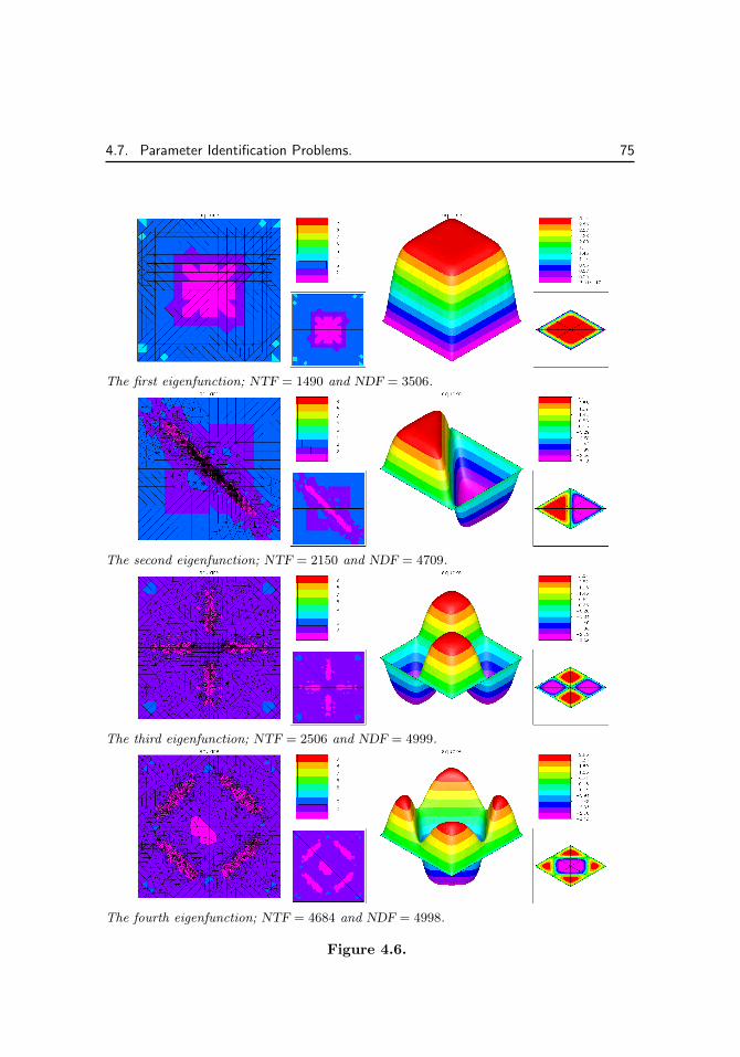
4.7. Parameter Identification Problems. 75
The first eigenfunction; NTF = 1490 and NDF = 3506.
The second eigenfunction; NTF = 2150 and NDF = 4709.
The third eigenfunction; NTF = 2506 and NDF = 4999.
The fourth eigenfunction; NTF = 4684 and NDF = 4998.
Figure 4.6.

76 PLTMG USERS’ GUIDE 13.0
Figure 4.7. The continuation path.
Here the matrix A is the Jacobian matrix corresponding the the bilinear forma(uh, vh). In particular, linear systems involving A (or At) are solved using thethe linear solver specified by METHOD. The matrix H is symmetric and has thesame sparsity pattern as A; other characteristics strongly depend on the particularproblem. Cu and Cv are NDF × NRL rectangular matrices, generally composedof NRL dense column vectors, and D is a NRL × NRL symmetric matrix. Thevectors δu and δv are the (Newton) updates for uh and the Lagrange multipliervh, respectively, and δλ is the update for λh. bu, bv and bλ correspond to theappropriate Newton residuals.
To describe the solution process for 4.11, we begin with the block factorizationH At CuA 0 CvCtu Ctv D
=
I 0 00 A 00 0 I
H I 0I 0 0Ctu Ctv D
I 0 Cv0 I Cu0 0 I
I 0 00 At 00 0 I
where
ACv = Cv,
Cu = Cu −HCv,D = D − CtuCv − CtvCu.
Computing Cv requires solving NRL linear systems with A. The two block diagonalmatrices each require solution of one linear system with A or At. Thus a total of2 + NRL elliptic pde systems need to be solved in each Newton step. The block

4.7. Parameter Identification Problems. 77
lower triangular system requires solving one dense linear system with the symmetricNRL×NRL matrix D.
The overall solution procedure is summarized below. Since the linear systemsinvolving A are generally solved only approximately by iteration, we introduce thematrix uλ ≈ Cv, that is generally the approximate Cv saved from the previousNewton step. This allows the computation of the current Cv to be done as anupdate with a residual-like right hand side. uλ is initially set to zero, and updatedwith the solution of every linear system.
First we solve
Abv = bv,
Aw = Cv −Auλ,uλ ← uλ + w,
Cv = uλ.
All linear systems involving A are (approximately) solved using the linear solverspecified by METHOD. Then we form
bu = bu −Hbv,Cu = Cu −HCv,
which requires sparse matrix multiplications with H. Next we compute δλ usingthe Schur complement
D = D − CtuCv − CtvCu,Dδλ = bλ − Ctubv − Ctv bu.
Finally, we form δu and δv from
δu = bv − Cvδλ,Atδv = bu − Cuδλ.
The latter requires the use of the linear solver for At. The basic Newton iterationis again that given in Figure 4.1 with the interpretation U t = (uth, v
th, λ
th) and
Gt = (btu, btv, b
tλ).
When IPROB = −4, a parallel Newton algorithm is implemented, similar instructure to the case IPROB = −1. A domain decomposition solver analogous tothat described in Section 4.4 is incorporated into the block elimination algorithmdefined above.
As an example, we consider the problem
min
∫Ω
∇u2 + δ
3∑i=1
λ2i dx,
subject to the boundary value problem and inequality constraints
−∆u = 1 in Ω
u = 0 on ∂Ω
λi ≤ λi ≤ λi, for 1 ≤ i ≤ 3.

78 PLTMG USERS’ GUIDE 13.0
The domain Ω is shown in Figure 4.8. The interior box is free to move withinthe domain, with its position governed by three parameters. (λ1, λ2) are the (x, y)coordinates of the center of the box and λ3 is its angle of rotation. This is the specialcase IPROB = 4 and ITASK = 8 allowing parameters to control the geometry ofthe domain.
The domain was provided as a skeleton and the initial mesh generated byTRIGEN. Both are shown in Figure 4.8. The optimization problem was then solvedon this mesh using piecewise linear elements. This first optimization step involvedsubstantial movement of the boundary, but the number of degrees of freedom wasrelatively small. Next, using alternating refinement and optimization steps, wecreated a final mesh with NDF = 22183 degrees of freedom. In each optimizationstep, the interior point parameter RMTRGT was reduced by a factor of 2 startingfrom its initial value of 1. While the boundary was allowed to move on all theseadditional optimization steps, it moved very little. In Figure 4.8, we also show thefinal solution, Lagrange multiplier, and the a posteriori error estimate computed onthe final mesh.
4.8 Optimal Control Problems.When IPROB = 5, PLTMG solves the control problem (1.13)-(1.16). This problemis similar to the case IPROB = 4 except that now λh is a finite element functionrather than a scalar. Here we consider the Lagrangian
L(uh, vh, λh) = ρ(uh, λh) + a(uh, vh)
− µNDF∑i=1
di
log(λh(pi)− λ(pi)) + log(λ(pi)− λh(pi))
(4.12)
where µ > 0 is the barrier parameter, di is the diagonal of the mass matrix corre-sponding to node pi, and vh is the Lagrange multiplier. As usual, our algorithmseeks a stationary point of the Lagrangian (4.12) using an approximate Newtonmethod.
The linear algebra problem at each Newton step is of the formH At SuA 0 SvStu Stv G
δuδvδλ
=
bubvbλ
. (4.13)
Here H and A are defined as before. In typical problems G is a symmetric, positivedefinite matrix, corresponding the regularization terms in (4.12). The matrix Galso has a nonnegative diagonal term arising from the inequality constraints forλh. As before, linear systems involving A and At are easily solved using the linearsolver specified by METHOD. Additionally, since G formally has the same sparsityas the stiffness matrix A, linear systems involving G are solved using a similarpreconditioning strategy. The matrices Su and Sv have the same symmetric sparsitystructure as G and A, but are generally not symmetric.

4.8. Optimal Control Problems. 79
The skeleton (left) and initial mesh with NTF = 132 and NDF = 82 (right).
The mesh after the first optimization step (left) and the final mesh with NTF = 4215 andNDF = 22183 colored by polynomial degree (right).
The final mesh colored by element size (left) and the solution (right).
The Lagrange multiplier (left), and the error estimate for the final mesh (right).
Figure 4.8.

80 PLTMG USERS’ GUIDE 13.0
Our solver is based on block Gaussian elimination, similar to the case IPROB =4. However, in the case of (4.13), it is too expensive to compute an exact Schurcomplement for the (3, 3) block; instead we approximate the Schur complement byG itself. Thus, our solution algorithm is just a preconditioner. In particular, it isone step of a block symmetric Gauss-Seidel iteration. This is realized as follows:
Acu = bv,
Atcv = bu −Hcu,Gδλ = bλ − Stucu − Stv cv,Aδu = bv − Svδλ,Atδv = bu −Hδu− Suδλ.
Linear systems involving A, At, and G are solved using the appropriate linearsolver. If G were replaced by the Schur complement and all linear systems solvedexactly, this would yield the exact solution. This approximate solver is used a thepreconditioner for the composite step conjugate gradient iteration.
When IPROB = −5, a parallel Newton algorithm is implemented, similar instructure to the case IPROB = −1. A domain decomposition solver analogous tothat described in Section 4.4 is incorporated into the block preconditioner definedabove.
As an example, we solve the optimal control problem
min
∫Ω
(u− u0)2 + β(∇u−∇u0)2 + γλ2 dx
subject to the constraint equation
−∆u = λ in Ω ≡ (0, 1)× (0, 1),u = 0 on ∂Ω,
and the inequalities1 ≤ λ ≤ 10.
The target function u0 was
u0 = sin(3πx) sin(3πy),
β = 10−2, and the regularization parameter γ = 10−4.This problem was solved in parallel using 16 processors, starting from an initial
uniform 17 × 17 mesh and piecewise linear elements. This mesh was adaptivelyrefined to NTF = 13700 elements and NDF = 6935, and partitioned, as illustratedin Figure 4.9. Each processor went through five iterations of adaptive refinement,with MXORD = 1, so that only piecewise linear polynomials were used. Thisproduced a global mesh with NDG = 450796 and block 3×3 linear systems of order1352388. The interior point parameter µ = µ0 = 10−2 on the 17 × 17 mesh, andthereafter was reduced by a factor of 2 in each refinement step, for a final size ofµ ≈ 1.4× 10⁻⁴.

4.8. Optimal Control Problems. 81
The final global mesh, colored by element size, is shown in Figure 4.9. InFigure 4.9, the solution (state variable), the Lagrange multiplier, the control λ, andthe error estimate are also shown. Note that PLTMG chooses only one approxima-tion space that is used for all three functions. Also all three functions contributeto the error estimate used in the adaptive procedure. The fact that the control λ isessentially a piecewise constant, while the other two functions are relatively smoothis likely responsible for the observed refinement pattern.

82 PLTMG USERS’ GUIDE 13.0
The initial 17× 17 mesh (left) and the load balance with NTF = 13700 (right).
The global refined mesh with NDG = 450796 colored by size (left) and the convergencehistory of the Domain Decomposition solver (right).
The solution u (left) and the Lagrange multiplier v (right).
The control λ (left) and the error estimate on the final mesh (right).
Figure 4.9.

Chapter 5
Graphics
5.1 Overview.The graphics package associated with PLTMG is composed of subroutines TRIPLT,INPLT, and GPHPLT. These routines are written in self-contained, portable For-tran, addressing the graphics output device through subroutines PLINE, PFILL,PFRAME, and PLTUTL. The specifications for these routines are given in Sec-tion 6.12.
Typical graphics output consists of three windows or frames. There is a largesquare window on the left, and two smaller square windows on the right. Themain image typically appears in the large frame, and other useful information (forexample, a legend matching colors to function values) appears in the smaller frames.The graphics interface provides z-buffer information, for use in three dimensionalimaging systems such as OpenGL. All the graphics routines are written such thatthe image appearing in the main window can be animated using such graphicssystems when appropriate.
Subroutine TRIPLT graphs the solution and various associated functions (e.g.,u, ψr, εt). TRIPLT also has options for plotting vector functions (e.g., ∇uh).Subroutine INPLT can display either a triangulation or a skeleton, with elements orregions colored according to various attributes such as the quality of the elements ina triangulation. Subroutine GPHPLT displays various graphs and charts containingtimings, convergence histories, and other items of interest.
The parameter MXCOLR is a device dependent constant, stating the max-imum number of colors available for use by the graphics package. We assumethat 2 ≤ MXCOLR. While it is possible to make some interesting plots andcontour maps with TRIPLT using only monochrome devices (MXCOLR = 2),TRIPLT makes extensive use of available color facilities in producing (shaded)three-dimensional surface plots and vector plots. GPHPLT and INPLT also usecolor, but in less critical ways.
Subroutines TRIPLT, INPLT and GPHPLT offer some capabilities for parallelprocessing. In the parallel processing environment, only the master process (corre-
83

84 PLTMG USERS’ GUIDE 13.0
sponding to IRGN = 1) makes calls to the graphics interface routines (PLTUTL,PFRAME, PLINE, and PFILL. However, in the case of TRIPLT or INPLT, onemay wish to plot the solution, error, or some other function in situations where thedata is distributed among the processors. If MPI is turned on (MPISW = 1), andMPIRGN = 0, then TRIPLT and INPLT collect data from all other processors,and draw a composite picture consisting of the union of the refined regions for eachprocessor. If the problem is sufficiently large that it is impossible or inefficient tocollect all the data on a single processor, each processor can coarsen its data beforesending it to the master process. This coarsening process is controlled by the pa-rameters ICRSN and ITRGT. If MPI is turned off (MPISW = −1), then TRIPLTand INPLT draw the function on processor one (refined in region one and coarseelsewhere). If one wishes to see the complete image as its exists on some otherprocessor, say processor I, set MPISW = 1, MPIRGN = I, and call TRIPLT orINPLT. For some options, GPHPLT collects data from all processors when MPI isturned on, for example in presenting timing and load balancing data.
For most of the examples of graphics output, we solved Laplace’s equationin a circle of radius one with a crack along the positive x axis. This domain wasused to illustrate the triangulation data structure in Section 2.3. NonhomogeneousDirichlet boundary conditions were imposed on the circular boundary such that thetrue solution is u = r1/4 sin(θ/4), the leading term in the singularity due to thecrack tip. Some example output in Section 5.4 came from other problems, in caseswhere it could not be provided by our simple example.
5.2 Subroutine TRIPLT.TRIPLT is called using the statement
Call TRIPLT( VX, VY, SF, ITNODE, IBNDRY, ITDOF, E,IP, RP, SP, GF, QXY, SXY )
The arrays VX, VY, SF, ITNODE, IBNDRY, and ITDOF should define atriangulation. GF and E contain functions for potential display. TRIPLT usesseveral variables from the IP, RP, and SP arrays, as shown in Tables 2.6–2.8. Thestring variable FTITLE is the character string displayed as a label above the graph.Additionally, TRIPLT can use the Fortran subroutine QXY. Subroutine QXY isdocumented in Section 2.8. The error flag IFLAG is set as in Table 2.9.
The parameter IFUN specifies the function to be plotted. The available op-tions are summarized in Table 5.1. Some of these functions are not defined forall problem types. Although there are many possibilities for IFUN, they may beclassified as surface plots and vector plots.
For surface plots, all functions are continuous with the (possible) exceptions ofthe error and scaling factors, which are piecewise constant on triangles, and QXY,which can be multivalued along element boundaries due to discontinuities in ∇uh.If desired, a discontinuous function can be mapped to a continuous function usinga local averaging technique. This is invoked by setting the switch ICONT = 1.

5.2. Subroutine TRIPLT. 85
Figure 5.1. The solution IFUN = 0 and the error IFUN = 5.
Figure 5.2. The case IFUN = 0, (NX,NY,NZ) = (1,−1,−1), andIFUN = 5, (NX,NY,NZ) = (1, 1, 1).
Figure 5.3. The case IFUN = 0, (NX,NY,NZ) = (1,−1,−1), RMAG =2, CENX = .5, CENY = .3, and the case IFUN=5, (NX,NY,NZ) = (0, 0, 1),RMAG = 2, CENX = .5, CENY = .3.
Figure 5.4. The case LINES = 1 and the case LINES = 3. The corre-sponding picture for LINES = 0 is in Figure 5.1.

86 PLTMG USERS’ GUIDE 13.0
Figure 5.5. The case IFUN = 2, ICONT = 1. (NX,NY,NZ) = (0, 0, 1)and (NX,NY,NZ) = (1, 1, 1).
Figure 5.6. The case IFUN = 1, ICONT = 1. (NX,NY,NZ) = (1, 1, 1).In the picture on the right RMAG = 2, CENX = .5, and CENY = .3.
Figure 5.7. Triangles colored by label (INPLSW = 0) and by quality(INPLSW = 2).
Figure 5.8. Triangles colored by size (INPLSW = 6) and by polynomialdegree (INPLSW = 5).

5.2. Subroutine TRIPLT. 87
IFUN displayed function
0 the solution uh1 the scalar function | ∇uh |2 the vector function ∇uh3 the alternate function QXY4 the alternate vector function QXY5 the error estimate ||εt||H1(t)
6 the tangent function u7 the right singular vector ψr8 the left singular vector ψ`9 the Lagrange multiplier um10 the control variable λh11 the dual function ω12 the scaling factor αt
Table 5.1. The values of IFUN.
5.2.1 Surface Plots.
In the case of surface plots, NCON specifies the number of contours (colors) to beused. If NCON > MXCOLR− 2, some colors are used for more than one contour.The parameters SMIN and SMAX can be used to specify the limits of the colorscale. If SMIN < SMAX , then these values are used as limits, with parts of thefunction lying outside (SMIN ,SMAX) colored white. Otherwise, the largest andsmallest values of the displayed function are used as limits.
Each picture consists of three frames; a large plot on the left and a two-partlegend on the right. The upper right contains a scale relating colors to function val-ues; three scales are available using the switch ISCALE as described in Section 5.2.4.For the case IFUN = 5, ICONT = 0, a histogram showing the distribution of errors||εt||H1(t) is also provided in this legend. Five line-drawing options using LINES andeleven labeling options using NUMBRS are also available. RMAG, CENX, andCENY provide a zoom-in capability as described in Section 5.2.3.
The main image can be animated using three dimensional imaging systemssuch as OpenGL. The viewing perspective can be statically set as well, using thetriple d = (NX ,NY ,NZ). The three-dimensional surface is projected into theplane orthogonal to d, and the function is drawn as it would appear to an observerviewing the surface from a line of sight parallel to d. The vectors (NX ,NY ,NZ)and −(NX ,NY ,NZ) cause the same projection to be computed; however, differentpictures are generally produced for the two cases. In the former case one observesthe projection on the “front” of the plane, and in the latter case one observes theprojection on the “back” of the plane. If MXCOLR is sufficiently large, the surfacewill be shaded relative to a light source directly behind the viewer, imparting someadditional three-dimensional character to the picture.
The lower right-hand legend provides guidance in understanding three-dimensional

88 PLTMG USERS’ GUIDE 13.0
surface plots. In this case the legend contains a “flat” version of the main picture, al-lowing another avenue for orienting oneself with respect to the viewing perspective.Some examples of surface plots are given in Figures 5.1–5.4.
5.2.2 Vector Plots.
Color plays an important role in the vector plots. Different colors correspond to dif-ferent directions in the vector field. This is illustrated in the color wheel portion ofthe upper right-hand legend. The number of directions is specified by the parameterNCON . Different intensities of the same color correspond to the magnitude of thevector; darker shades correspond to smaller magnitudes, and lighter shades corre-spond to higher magnitudes. The correspondence between color intensity and vectormagnitude is illustrated for an example color in the upper right-hand legend. Theparameters SMIN and SMAX are used to specify the limits of the color intensityscale for the magnitude of the vector. As with surface plots, if SMIN < SMAX,then these values are used as limits; otherwise the largest and smallest magnitudesof the vector function are used.
Three scales for the vector magnitude are available using the option switchISCALE. Five line-drawing options using LINES and eleven labeling options usingNUMBRS are also available, and RMAG, CENX, and CENY provide zoom-incapabilities. The triple (NX,NY,NZ) specifies a direction as in the case of surfaceplots. In this case the surface plotted is the linear interpolant of the magnitude of thevector function.9 In this case the elements remain colored as in a two dimensionalvector plot. Some examples of vector plots are given in Figures 5.5 and 5.6.
5.2.3 Parameters RMAG, CENX, and CENY.
The parameters RMAG, CENX, and CENY provide a zoom-in option. RMAGis the magnification factor relative to the picture coordinates. For example, ifRMAG = 1 the whole picture will be drawn; if RMAG = 2, the picture is scaled bya factor of 2 in both directions and thus no longer fits on the output device. Onemust now choose a window and view only a portion of the picture. The fractions0 ≤ CENX ≤ 1 and 0 ≤ CENY ≤ 1 are used for this purpose. In particular(CENX ,CENY ) specifies the point that will appear at the center of the magnifiedwindow. If RMAG = 1, the values of CENX and CENY are ignored. Someexamples are shown in Figure 5.3 and Figure 5.6 (right).
As an aid to understanding, the lower right legend contains a copy of thecomplete picture (corresponding to RMAG = 1). Whenever RMAG > 1, a smallbox is drawn in this legend depicting the portion of the picture appearing in themain graph. The box is supplemented by a crosshair locator, since the box becomestoo small to be visible for large magnification factors.
9 For the actual magnitude, the surface of each triangular element is not necessarily a plane,making the hidden surface problem more difficult.

5.2. Subroutine TRIPLT. 89
5.2.4 Parameters ISCALE, LINES, NUMBRS, and MPIRGN.
The parameter ISCALE provides three scaling options, summarized in Table 5.2.For linear scaling, drawn contours are equally spaced with respect to the largest andsmallest values of the given function z(x, y). If ISCALE = 1, then the contours areequally spaced with respect to the largest and smallest values of log z. If ISCALE =2, then the contours are equally spaced with respect to largest and smallest valuesof the function sinh−1z. The logarithmic scaling clearly requires z to be positive.The sinh−1 scaling is always defined, having a (signed) logarithmic behavior forlarge | z | and a linear behavior for small | z |. If ISCALE = 1 and z ≤ 0 at somenode, then TRIPLT defaults to the sinh−1 scaling. In Figure 5.1, the solution uhwas drawn using the linear scale (ISCALE = 0), while the error estimate was drawnusing the logarithmic scale (ISCALE = 1).
Five line drawing options are available, specified through the parameter LINES,as summarized in Table 5.2. If LINES = 0, TRIPLT will draw edges of all trianglesin the mesh. If LINES = 1, only boundary edges and edges separating trian-gles from different regions are drawn. The case LINES = 2 is similar to the caseLINES = 1, except that here boundary edges and edges separating triangles fromdifferent processors are drawn. When LINES = 3 for surface plots, TRIPLT drawsboundary triangle edges and contour lines separating contours of different colors.This option produces a traditional contour map on monochrome devices and thusis useful when MXCOLR = 2. Some examples for LINES = 1 and LINES = 3 areshown in Figure 5.4. The option LINES=3 is not implemented for vector plots. Theoption LINES=-1 displays the underling (typically refined) graphics triangulationthat was actually used by TRIPLT in making the image; this is mainly of interestfor debugging.
Eleven labeling options are available in TRIPLT; these are specified throughthe parameter NUMBRS, as summarized in Table 5.2. When NUMBRS 6= 0, three-dimensional plotting is disabled; the result will be a “flat” (but labeled) surface.Some examples are shown in Figures 2.1 and 2.2.
In making images using MPI, the usual situation is that each processor con-tributes its part of the image, corresponding to its refined subdomain. However, incertain situations (such as debugging), one may wish to see the complete image asit exists on an individual processor. The parameter MPIRGN allows this. WhenMPIGRN = 0, its default value, then all processors contribute to a given image inthe usual way. When MPIGRN = I for 1 ≤ I ≤ NPROC , then the complete imagefrom processor I is drawn.
5.2.5 Parameters ICRSN and ITRGT.
When NDF becomes very large, the amount of data used to make an image maybecome too large for animated display systems like OpenGL or for Postscript files ofreasonable size.10 In this situation, one may wish to compress the data and make alower resolution image. The parameter ICRSN indicates whether or not to coarsen
10Raster graphics images like those produced by XPM files are largely independent of the sizeof the underlying data set.

90 PLTMG USERS’ GUIDE 13.0
ISCALE scale
0 linear1 logarithmic
2 sinh−1
LINES line drawing option
0 all triangle edges1 boundary/interface edges2 load balance boundary edges3 contours-1 underlying graphics triangulation
NUMBRS labeling option
0 no labels1 triangles/subregions2 vertices3 edges4 curved edges5 edge type6 edge labels7 processor8 vertex type9 degrees of freedom10 element degree
MPIRGN image option
0 all processors contributeI > 0 draw image from processor I
ICRSN coarsening option
0 no coarsening1 coarsen global subspace
ICONT smoothing option
0 no smoothing1 smooth piecewise constant function
Table 5.2. The values of ISCALE, LINES, NUMBRS, MPIRGN, ICRSN,and ICONT.
the global subspace, as indicated in Table 5.2. If ICRSN = 1, then the parameterITRGT specifies the target number of degrees of freedom for the coarsened subspace.The coarsening option is very much like the mesh coarsening option in TRIGEN ;many of the same subroutines are used, and the overall coarsening strategy is thesame. However, the coarsening criteria is different. When MPI is on (MPISW = 1),

5.3. Subroutine INPLT. 91
each processor independently coarsens the subspace for its subregion to a target ofITRGT/NPROC degrees of freedom. Thus, when the subspaces are later combined,the global subspace appearing in the image will have at most ITRGT degrees offreedom.
When the mesh is coarsened, all numbering options are disabled; NUMBRS =0 is always used. The setting LINES = 0 is reset to LINES = 1, and ICONT = 1is always used.
5.2.6 Some Algorithmic Details.
The main algorithms of interest in TRIPLT are those for hidden line and surfaceremoval. In the general case of a surface plot, one must make comparisons betweenvarious triangles to determine whether a given triangle blocks another with respectto the viewer. Since the triangular mesh is generally unstructured, our goal is toorganize the data to minimize the number of comparisons between triangles.
Generally, for surface plots in which (NX ,NY ,NZ) 6= (0, 0, 1), a partial orderis constructed in which elements farthest from the viewer are ordered first, and thoseclosest to the viewer are ordered last. The elements are then drawn and colored inorder, with the elements closer to the viewer (possibly) overwriting some elementsthat are farther away. The notion of distance from the viewer is defined with respectto the x and y coordinates only, so that the same ordering is computed independentof the function being graphed. A typical element is compared only to elements withwhich it shares a common edge; it is ordered before any edge neighbors closer to theviewer and after any neighbors farther away. Since any element has at most threeneighbors, this greatly limits the number of comparisons necessary and completelysolves the ordering problem for a convex domain with no holes.
Unfortunately, many domains are not convex and have holes, so that elementswith boundary edges must be treated as special cases. Thus we make a list oftriangles with boundary edges, sort them with respect to the direction (in the(x, y) plane) perpendicular to the (NX ,NY ) components of the viewing direction.Boundary edges are also sorted by whether they face “backward” or “forward”with respect to (NX ,NY ). With these preliminary calculations done, all pairs ofrelevant triangles that might conflict are tested and appropriate ordering constraintsimposed. For a mesh with NTF triangles, the number of boundary triangles isO(√NTF), so that in the worst case (every boundary element compared with every
other boundary element), this will still be only O(NTF) work. Since only O(NTF)work is required for the interior elements, the overall work is still O(NTF).
5.3 Subroutine INPLT.Subroutine INPLT is a graphics routine for displaying the input data defining atriangulation or a skeleton. INPLT is called using the statement
Call INPLT( VX, VY, SF, ITNODE, IBNDRY, ITDOF,IP, RP, SP, SXY )

92 PLTMG USERS’ GUIDE 13.0
The arrays VX, VY, IBNDRY, ITNODE, and SF define either a triangulationor a skeleton (INPLT uses the value of ITNODE(3,1), which is zero for a skeletonand positive for a triangulation, to distinguish these cases). The string variableITITLE is displayed as a banner above the graph. Variables in the IP, RP, andSP arrays used by INPLT are shown in Tables 2.6–2.8. INPLT was used to makeFigures 3.1 3.8, and 3.9, among others in this manual.
INPLSW triangulation skeleton
0 user label user label1 load balance subregion2 element quality3 largest angle4 smallest angle5 mesh grading6 polynomial degree7 element diameter
Table 5.3. The values of INPLSW.
5.3.1 Triangle Plots.
For triangle plots, the elements in the triangulation are colored to depict somefeature of the mesh. The available options are controlled by the switch INPLSWas summarized in Table 5.3.
If INPLSW = 0, the elements in the mesh are colored according to the usersupplied labels in ITNODE(5,I); all elements with the same label will have the samecolor. If INPLSW = 1, the elements in the mesh are colored according to the loadbalance (ITNODE(4,I)).
For 2 ≤ INPLSW ≤ 5, INPLT colors the elements of the triangulation ac-cording to their quality, measured by q(t) in (3.1), their largest angle, their smallestangle, and the local mesh grading, respectively. For each of these measures, fivenumbers are printed in the upper right legend. The row labeled “average” refers tothe average of that quantity over all elements in the mesh; “worst” reports the small-est value of q(t), largest angle, smallest angle, or the steepest local grade over all ofthe elements. The rows labeled “good,” “fair,” and “poor” report the percentageof elements in each category and depict the corresponding colors.
For q(t), good means q(t) ≥√
3/2, fair means .6 ≤ q(t) <√
3/2, and poormeans q(t) < .6. For large angles, good means A(t) ≤ π/2, fair means π/2 < A(t) ≤2π/3, and poor means A(t) > 2π/3 (A(t) is the largest angle). For small angles,good means arccos(4/5) ≤ a(t), fair means arccos(13/14) ≤ a(t) < arccos(4/5) andpoor means a(t) < arccos(13/14) (a(t) is the smallest angle). Triangles that aregood in terms of q(t) are (necessarily) also good in terms of large and small angles.Those that are fair in terms of q(t) must be good or fair in terms of large and small

5.3. Subroutine INPLT. 93
angles (but not conversely). The local mesh grading gv at any vertex v in the meshis the ratio of the largest to smallest lengths among all the element edges having vas an endpoint. The mesh grade for an element g(t) is the maximum of gv among itsthree vertices. For mesh grading, good means g(t) < 2, fair means 2 ≤ g(t) ≤ 3 andpoor means g(t) > 3. In Bank and Yserentant [39], control of mesh grading is seento be a crucial point in creating nonuniform meshes where the L2(Ω) projection ofa function u ∈ H1(Ω) is stable in the H1(Ω) norm.
When INPLSW = 6, INPLT produces an image in which each element iscolored according to its polynomial degree. A histogram showing the distributionof element degrees appears in the legend. When INPLSW = 7, INPLT producesan image in which each element is colored according to its size. A histogram show-ing the distribution of element sizes appears in the legend. Although any scalingoption available through ISCALE can be used, generally the logarithmic scaling(ISCALE = 1) produces the most useful image. Some example images made usingINPLT are shown in Figures 5.7 and 5.8.
The meanings and use of RMAG, CENX , CENY , and MXCOLR are identicalto TRIPLT. Labeling options using NUMBRS are summarized in Table 5.2. INPLTwas used with various NUMBRS options to produce Figure 2.1 although the legendson the right-hand sides of the pictures were deleted. For the main graph, three line-drawing options are available using LINES, as summarized in Table 5.2.
The meaning and use of parameter MPIRGN is the same in subroutine INPLTas in TRIPLT. Subroutine INPLT also allows mesh coarsening, but the criterionis different. In INPLT, each element is a single color and the images are two di-mensional, and the coarsening criterion reflects these differences. As with TRIPLT,NUMBRS = 0 is always specified for a coarsened mesh and LINES = 0 is reset toLINES = 1.
5.3.2 Skeleton Plots.
As with triangle plots, the subregions of the skeleton are colored according to theoption specified by INPLSW as summarized in Table 5.3. If INPLSW = 0, thesubregions are colored according to the user supplied labels in ITNODE(5,I), similarto the case of a triangulation. If INPLSW = 1, each subregion is given a differentcolor.
Subroutine INPLT draws a skeleton by first creating a crude triangulationbased on the skeleton, and then drawing the triangulation. Here shape regularityand overall quality of the triangulation is not an issue; rather, keeping the number ofelements small and computing the triangulation quickly are important. The optionLINES = −1 displays the underlying triangulation used in the skeleton plot. It wasincluded mainly for debugging purposes.
The parameters RMAG, CENX , CENY , and MXCOLR are the same as fortriangle plots. Labeling options using NUMBRS are summarized in Table 5.2.There are no coarsening or parallel computation options available for skeleton plots.INPLT was used with various NUMBRS options to produce Figure 2.2.

94 PLTMG USERS’ GUIDE 13.0
5.4 Subroutine GPHPLT.Subroutine GPHPLT displays an assortment of data related to the performanceof various algorithms and subroutines in PLTMG and TRIGEN using a graphicalformat.
GPHPLT is called using the statement
Call GPHPLT( IP, RP, SP )
GPHPLT makes use of the arrays TIME and HIST, that reside in a commonblock initialized by PLTMG and TRIGEN when IFIRST 6= 0. The string variableGTITLE is displayed as a banner above the graph. Other variables in the IP, RP,and SP arrays used by GPHPLT are shown in Tables 2.6–2.8.
IGRSW displayed graph
0 Newton iteration convergence history1 CSCG/CSBCG iteration convergence history-1 matrix statistics2 individual subroutine timing statistics-2 time pie chart3 the continuation path-3 load balance4 error estimates for H1 norm-4 error estimates for L2 norm5 the IP array-5 the SP array6 the RP array
Table 5.4. The values of IGRSW.
IGRSW is an integer switch for selecting the displayed graph; the availablepossibilities are summarized in Table 5.4.
5.4.1 Iteration Information.
For the cases IGRSW = −1, 0, 1, information about various iterations and precon-ditioners is displayed. In all three cases, the same three graphs are drawn. The largemain window contains the information indicated in Table 5.4 for the correspondingvalue of IGRSW. The other two graphs appear in the two smaller frames on theright. Examples are shown in Figures 5.9– 5.10.
In the case IGRSW = 0, in the main window GPHPLT graphs the functions
Rk = log10
||Gk||||G0||
and Ek = log10
||δUk||||Uk||
.
Gk is the residual for the Newton iteration, while δSk is the incremental change in

5.4. Subroutine GPHPLT. 95
Figure 5.9. The cases IGRSW = 0 and IGRSW = 1.
Figure 5.10. The cases IGRSW = −1 and IGRSW = 4 with(MX,MY,MZ) = (1,−1, 1).
Figure 5.11. The cases IGRSW = 2 and IGRSW = −2.
Figure 5.12. The cases IGRSW = 3 and IGRSW = −3.

96 PLTMG USERS’ GUIDE 13.0
Figure 5.13. The cases IGRSW = 5 and IGRSW = 6.
Figure 5.14. The case IGRSW = −5.
the solution Sk. The precise meaning of Gk and Sk varies according to the systemof nonlinear equations solved for each problem class addressed by PLTMG. Bothconvergence histories are plotted in a bar graph of Rk and Ek versus iteration indexk. The convergence history for the most recently solved set of equations is displayed.When this corresponds to a regular (serial) solution (IPROB > 0), the relativeresiduals are red bars, while the solution increments are blue. At most, informationabout the last twenty Newton iterations is displayed. When IPROB < 0, theNewton iteration employs the parallel domain decomposition solver in place of thesimple preconditioned linear solver. In this case, the residuals are magenta bars,and the solution increments are cyan.
Nominally, the rate of convergence for Newton’s method should asymptoti-cally be quadratic; however, the convergence becomes linear when systems of linearequations involving the Jacobian matrix are only approximately solved.
In the case IGRSW = 1, in the main window GPHPLT graphs the function
S(k) = log10
||rk||||r0||
.
Here rk is the residual of a set of linear equations to be solved and k is the iterationnumber. The displayed histories are for linear systems solved in the most recentNewton iteration. Up to four such systems are solved in each Newton step, depend-ing on the value of IPROB. In all cases, only information about the last twentyiterations is saved and displayed.

5.4. Subroutine GPHPLT. 97
Either the composite step conjugate gradient method or composite step bi-conjugate gradient method is used [10, 9], preconditioned by the solver specified byMETHOD. Each individual step is marked with a small icon; a color pair (green,red), (blue, yellow), (cyan, magenta), (white, black) is assigned to each history. Ineach case, for simple steps the icon is colored with the first color (e.g., green), whilefor composite steps the icon is colored with the second color (e.g., red).
In the case IGRSW = −1, in the main window statistics related to the thesparse matrix and its factorizations is displayed. Potential information about fivematrices is given
1. The stiffness matrix, colored yellow.
2. The ILU factorization, colored green.
3. The HB factorization, colored cyan.
4. The block diagonal factorization, colored blue.
5. The complete LU factorization, colored magenta.
The first four correspond to matrices and factorizations that have been computed;ILU and HB and block diagonal factorization data appear only if they have beenselected by the parameter METHOD. The complete LU factorization data is in-cluded for reference, and indicates data relevant to sparse Gaussian Eliminationwith the minimum degree ordering.
At the top, two columns of figures appear. The first is the average number ofnonzeros per row in the matrix. The second is the same, but given as a percentagerelative to sparse Gaussian Elimination. Below is a bar graph reflecting the actualstorage used. This is different from the numerical data, in that if the matrices aresymmetric, only the diagonal and upper triangle are stored. The storage bar forGaussian Elimination (LU) is hypothetical only. In each colored bar, a verticalblack line might appear; this indicates the size of the JA or JU arrays relative tothe corresponding A or U arrays.
5.4.2 Timing Statistics.
If IGRSW = 2, GPHPLT prints a summary of timing statistics for PLTMG andTRIGEN. An example is given in Figure 5.11. Statistics are given both for thetotal accumulated time since initialization (IFIRST = 1) and for the time spentduring the last call to PLTMG or TRIGEN. The timings are itemized with respectto subroutines that carry out major computational tasks in the package. Thesesubroutines are listed in Table 5.5. Depending on the problem, some of theseroutines may not be called.
A bar graph is drawn illustrating the percentage of time spent in each routine.Each bar in the graph is partitioned into a part corresponding to the last call toPLTMG (red) and a part corresponding to all preceding calls (blue). The timingpie graph described below appears in the upper right frame.

98 PLTMG USERS’ GUIDE 13.0
If IGRSW = −2, GPHPLT displays a pie graph summarizing the same infor-mation. Each routine in Table 5.5 is assigned to one of six categories: linear systemassembly (red), multigraph solver (green), mesh generation (magenta), a posteriorierror estimation (cyan), parallel processing routines (yellow), and other PLTMGroutines (blue). A pie graph showing the fraction of total time spent in each ofthe six categories is drawn in the main frame. Details of individual contributionsfrom the subroutines listed in Table 5.5 are summarized in the upper right frame.Sample output is shown in Figure 5.11.
When MPISW = 1, the times displayed for IGRSW = ±2 are time averagedacross all processors. In this case, in the lower right frame, a graph displaying thedeviation from the average time for each processor is drawn.
5.4.3 Continuation Path.
When IGRSW = 3, GPHPLT displays the continuation path generated by thecontinuation procedure IPROB = 3. Target points are marked by small boxes,generally using different colors for different values of ITASK. A legend appears inthe upper right frame summarizing the possibilities. Up to one hundred targetpoints generated by calls to PLTMG are saved and displayed. Successive pointsare interpolated using parabolic arcs matching the values of (λ, ρ) and the tangentvectors (λ, ρ). In the lower right frame appears a convergence history for the mostrecent singular vector computation. Sample output is shown in Figure 5.12.
5.4.4 Parallel Statistics
When IGRSW = −3, GPHPLT plots the functions
Tk = log2
NPROC ·NTF (Ωk)∑
kNTF (Ωk)
and Ek = log2
NPROC||εt||H1(Ωk)∑
k ||εt||H1(Ωk)
where 1 ≤ k ≤ NPROC. Both curves appear in the large frame. When MPISW =1 the information from all processors is obtained by an exchange of data usingthe MPI library. This is the most useful situation. When MPISW = −1, thesame graph is made using local data on the given processor; this case is typicallynot interesting. In the upper right frame is a similar graph for the distribution oferror and elements following the initial load balancing step (IADAPT = 7). In thelower right frame appear convergence histories for eigenvalue computations in theload balancing phase. Convergence histories are shown for the four most recentproblems. Sample output is shown in Figure 5.12.
5.4.5 Error Estimates.
In the case IGRSW = 4, GPHPLT graphs the function
F1(NDF,TIME) = log10
||εt||H1(Ω)
||uh||H1(Ω)
,

5.4. Subroutine GPHPLT. 99
and in the case IGRSW = −4, GPHPLT graphs the function
F0(NDF,TIME) = log10
||εt||L2(Ω)
||uh||L2(Ω)
.
Here εt is the computed approximation of the error u − uh. While it is hopedthat these approximations accurately reflect the true state of affairs, the estimatesare based on a posteriori calculations involving only the computed solution. Somejudgment of the validity of such computations may be required. An example isshown in Figure 5.10.
Error estimates are plotted as a function of both NDF and TIME. In partic-ular, Fj is graphed versus log10NDF and log10TIME in a three-dimensional graph.All data points (up to the 20 most recent) for which error estimates are availableare marked with rectangular cylinders of different colors. A legend appears in theupper right frame summarizing the possibilities. In the case IGRSW = 4, the plotof F0 appears in the lower right frame; if IGRSW = −4, the plot of F1 in the lowerright frame.
The triple d = (MX ,MY ,MZ) specifies the viewing perspective for thesegraphs in a fashion similar to (NX,NY,NZ) for surface plots. The choice (1,−1, 1)is a reasonable default. The choice (0,−1, 0) yields a traditional two-dimensionalgraph of log10 Fj versus log10 NDF. The choice (1, 0, 0) yields a two-dimensionalgraph of log10 Fj versus log10TIME. The main image can be animated using threedimensional imaging systems such as OpenGL.
5.4.6 Displaying Data Arrays.
The options | IGRSW |≥ 5, GPHPLT displays the IP, RP, or SP arrays. Unlikeother graphics options, here the entire graphics window is treated as a single frame.In the case of the IP and RP arrays, all 100 entries, their names, and their currentvalues are displayed. Entries that can be interactively reset in the ATEST driverare colored red, unused entries appear in black, and all other entries are coloredblue. This situation is similar for the SP array, except only the first 50 entriesare displayed (the remainder are all presently unused). Examples are shown inFigures 5.13–5.14.

100 PLTMG USERS’ GUIDE 13.0
subroutine main function
TGEN create triangulation from skeletonREFINE adaptively refine the triangulationUNREFN adaptively unrefine the triangulationHUNFRM uniformly h-refine the triangulationPUNFRM uniformly p-refine the triangulationMVEMSH adaptively smooth the mesh pointsERREST compute error estimates for uhCBUMP recover derivatives for error estimationCDLFN compute dual functionCNORMS compute global a posteriori error estimateEXPTH MPI exchange IPATH dataBCAST broadcast mesh to all processorsLDBAL compute a load balanceLDEV solve eigenvalue subproblem in load balanceCUTR reorganize data structures for reconciling meshPASTE reconcile mesh along interface of IRGNPASTE1 reconcile mesh along interface not part of IRGNTRIGEN all other time spent in TRIGEN
SETGRB compute block JA arraySETGR2 compute DD interface JA arrayJA2JA min degree / reorderingSFBILU block ILU factorizationSFHB HB matrix factorizationMG solve equations using CSCG/CSBCG iterationBLK3 solve equations for IPROB = ±3BLK4 solve equations for IPROB = ±4BLK5 solve equations for IPROB = ±5LINSYS assemble linear systemRGNSYS assemble linear system for DDCEV compute the singular value µ and vectors ψr and ψ`SWBRCH switch branches at a bifurcation pointPREDCT compute the steplength σ for continuationTPICK line search for Newton iterationTPICKD line search for Newton/DD iterationPLTMG all other time spent in PLTMG
Table 5.5. Subroutines timed by GPHPLT.
Chapter 6
Test Driver
6.1 Overview.Program ATEST is the test driver used in the development and testing of thePLTMG package. ATEST is a flexible program in that it accepts simple commandstrings directing it to call subroutines or perform other tasks. It is not limited toa fixed sequence of tasks on a particular run; any routine can be called as often asdesired, with certain parameters reset for each call at the discretion of the user.
The program ATEST can operate in four modes, governed by the switchMODE. If MODE = −1, ATEST runs as an interactive program, accepting com-mands from the user via a terminal window. If MODE = 0, ATEST runs interac-tively, accepting commands from the user via a web browser interface. The com-munication link between ATEST and the web browser is a socket, so that the clientweb browser can be running on a different device from the server running ATEST. IfMODE = 1, ATEST runs as a batch program, reading commands from a journal fileand sending all output to appropriate output files. Finally, if MODE = −2, ATESTruns as a slave mode under MPI; this mode cannot be directly set by the user, butis set by ATEST if it determines that it is a slave node in a parallel computation.In this situation, the user specifies MODE only for the master node, which can beany of the three other options. The value of MODE is set in a parameter statementat the beginning of ATEST, and also can be set dynamically in the command linelaunch of an ATEST application as described in Section 6.6.
A common command syntax is used for all modes. This is described first forthe case MODE = −1 in Section 6.2. The extensions used in the web browserinterface are described in Section 6.3.
Several files are written by ATEST. The file BFILE contains a complete recordof all commands and printed output produced during the session. The file JWFILEcontains a record of all commands read and processed during the session, formattedas a journal file. See Section 6.9 for a discussion of journal files. ATEST alsocreates a temporary file JTFILE used in connection with the journal command.While most commands invoke one of the major routines in the package, there are
101

102 PLTMG USERS’ GUIDE 13.0
a few utility routines (e.g. for reading and writing files) which are documented inSections 6.8–6.10.
6.2 Terminal Mode.In terminal mode, commands are entered from a terminal window in characterstrings of 80 characters, counting blanks. The syntax of a command can takeseveral forms, but the root command is always a single letter. The commands thatare currently recognized by ATEST are summarized in Table 6.1.
Command Action
s call PLTMGt call TRIGENf call TRIPLTg call GPHPLTi call INPLTr read data set from a filew write data set to a fileu call USRCMDj execute journal filep MPI toggleq quit
Table 6.1. Available commands for ATEST.
The terminal window prompt is the string command:. At this prompt, onecan enter a command string (e.g., s), reset parameters as described below, or entera blank line to see a list of the available commands. In this latter case the terminalwindow will appear as follows.
command:
pltmg s trigen t triplt f gphplt g inplt i read r
write w usrcmd u journl j mpi p quit q
command:
A syntax error in a given command string causes the entire string to be ignored.ATEST will display the string command error and present the command promptfor a new input string.
The most simple commands are just single lower case letters as shown inTable 6.1. However, associated with most commands are various parameters whichcan be reset before calling the given routine. To see a listing of the parametersassociated with a given command and their current values, without executing thecommand itself, enter the command in upper case at the command prompt. Forexample, the command F will display the parameters which can be interactivelyreset in connection with TRIPLT.

6.2. Terminal Mode. 103
command:F
ifun f 0 iscale s 0 lines l 0 numbrs n 0
idevce d 0 fpane p 0 ncon c 11 mxcolr mc 256
icont ic 0 nx nx 0 ny ny 0 nz nz 1
mpirgn mr 0 rmag m 1.0 cenx cx 0.5 ceny cy 0.5
smin sn 0.0 smax sx 0.0 icrsn cr 0 itrgt it 10000
ftitle t "alpha = 0.25"
grfile gf circle_figxxx.ext
command:
There are fifteen integer parameters, five real parameters, one string parame-ter, and one file parameter affecting subroutine TRIPLT that can be interactivelyreset by the user. To the right of each parameter is a one- or two-letter alias (toavoid typing long names), followed by the current value.
To reset some parameters associated with a command c (c = s, f, g, etc.),without invoking the command itself, one can type a string of the form
command:C name1=value1, name2=value2, ... , namek=valuek
Note that the root command appears in upper case. The namek refer to variablenames or their aliases, and valuek refer to integer, real, or string values. Severalparameters can be reset, with different entries separated by commas. Values forinteger parameters should be integers, while values for real parameters can be spec-ified using integer, fixed point, or exponential notation. There are three types ofstring parameters: short, long and file. Short strings are typically single words andcan not contain any blank characters. Files are typically file names, and they alsocan not contain any blank characters. All other strings are long, and can containany printable ASCII characters other than double quotes. Values of long string pa-rameters should appear within double quotes. Short and file string parameters arenot enclosed with double quotes. Blank spaces are ignored everywhere but withinthe value field of a long string parameter. A syntax error in the input line (e.g.,a misspelled variable name) causes the entire command to be ignored and no vari-ables to be reset. ATEST will respond command error and then ask for the nextcommand. For example, here we reset ISCALE = 1, NCON = 20, CENX = .3,RMAG = 10, and FTITLE = A new title for Circle. Subroutine TRIPLT is notcalled, but the parameters are updated and redisplayed as
command:F s=1, ncon=20, cenx=.3, rmag=1.e1, t="A new title for Circle"
ifun f 0 iscale s 1 lines l 0 numbrs n 0
idevce d 0 fpane p 0 ncon c 20 mxcolr mc 256
icont ic 0 nx nx 0 ny ny 0 nz nz 1
mpirgn mr 0 rmag m 10.0 cenx cx 0.3 ceny cy 0.5
smin sn 0.0 smax sx 0.0 icrsn cr 0 itrgt it 10000
ftitle t "A new title for Circle"
grfile gf circle_figxxx.ext
command:
One can reset some parameters for a given command c, and then invoke thecommand itself, using a string of the form

104 PLTMG USERS’ GUIDE 13.0
command:c name1=value1, name2=value2, ... , namek=valuek
Note that the only difference is that the root command now appears in lower caserather than upper case. Thus
command:f s=1, ncon=20, cenx=.3, rmag=1.e1, t="A new title for Circle"
resets the indicated parameters as in the previous example. However, instead ofdisplaying the updated values, subroutine TRIPLT is called.
Finally, the graphics and MPI commands (f , i, g, and p) have a short form al-lowing one crucial parameter (IFUN, INPLSW, IGRSW, and MPISW, respectively)to be reset without typing even the alias. For example,
command:f5
is the short form for
command:f ifun=5
The short and long forms of these commands cannot be mixed. Thus
command:f5, ncon=10
is not valid.
6.3 Web Browser Mode.When MODE = 0, the driver ATEST connects to a web browser interface via socketWEBPRT . While the WEBGUI browser interface was written by Chris Deotte tocontrol PLTMG, it was designed as a graphical user interface for any C or Fortranpackage. Complete documentation is provided in [47]; here we will mainly discussits use in PLTMG. When an ATEST application is launched with MODE = 0, itdisplays a message of the form
webgui: Listening on port 15000 for web browser...
In this example WEBPRT = 15000. To establish a connection with a web browserrunning on the same computer as the ATEST application, type
http://localhost:15000
in the web browser’s address bar. If the web browser is running on a different clientdevice, replace localhost with the IP address or the hostname of the computerrunning the ATEST application. Once the connection is established, the WEBGUIinterface should appear in the the web browser. The value of WEBPRT is set in aparameter statement at the beginning of ATEST and also can be set dynamicallyin the command line launch of an ATEST application as described in Section 6.6.

6.3. Web Browser Mode. 105
The functional capabilities of the web browser interface are the same as thosefor terminal window mode, but the possibilities for data entry are more varied. Anexample of the web browser interface interface appears in Figure 6.1. The webbrowser display has four main elements. There are three graphics panes, and inthe upper left is the main control panel. The graphics interface will be described inmore detail in Section 6.12.4. Here we discuss the main control panel.
Figure 6.1. The web browser interface.
The control panel contains two elements. The upper portion of the displaycontains command buttons. The bottom portion of the display is the history window.The command buttons stand in one to one correspondence with the basic ATESTcommand set shown in Table 6.1. To the right of each main command buttonis a smaller button labeled with a plus sign. Clicking on a command button isequivalent to the typed lower case version of the given command. For example,clicking on the button for the TRIPLT command causes subroutine TRIPLT tobe called as in the command f . Clicking on the plus button to the right of anycommand is equivalent to the typed upper-case version of that command. In this

106 PLTMG USERS’ GUIDE 13.0
case a drop down menu appears containing a display of all the parameters thatcan be modified by that command. For example, clicking on the plus button forthe TRIPLT command causes the parameters for the TRIPLT command to bedisplayed as in the command F . This is shown is figure 6.2.
Figure 6.2. Drop down menu for resetting parameters for TRIPLT.
The parameters associated with a given command are displayed in the resetwindow in a format similar to terminal mode. However, each parameter value isdisplayed in one line text-editing window, and can be reset by typing in the newvalue. Some parameter names (e.g., IFUN in Figure 6.2) appear in a button. Ifthe parameter is a switch with several options, clicking on the name button causesthe drop down menu to expand and display a suite of radio buttons indicatingthe various options associated with the parameter. Clicking on the desired optioncauses the parameter to be reset to the corresponding value. The radio buttonsassociated with the parameter IFUN appear in Figure 6.3.
On the other hand, if the parameter is a file name, clicking on the namebutton causes the drop down menu to display a file selection widget. The file-

6.3. Web Browser Mode. 107
Figure 6.3. Radio buttons for the parameter IFUN.
selection widget for the RWFILE associated with the READ command is shown inFigure 6.4.
The history window displays the contents of the output file, BFILE, as it iscreated. When executing a journal file in web browser mode, if a graphics commandis executed, depending on the graphics device selected, ATEST can pause after thepicture is drawn, and create a small popup click to continue button. In this case,ATEST waits until the user dismisses the click to continue popup before continuingto execute the journal file. This allows time for the user to view the picture beforeprocessing the next command in the journal file.
The WEBGUI interface has several additional features that are useful in cer-tain situations. These appear in Table 6.2. To use these features one presses theOPTION key (ALT key on Windows machines) while also pressing the indicatedkey. When OPTION + C are pressed, the command buttons disappear and are re-placed with a command line where commands may be entered as in terminal mode.Facsimiles of the displays created in terminal mode appear in the history window.

108 PLTMG USERS’ GUIDE 13.0
Figure 6.4. File sector for the parameter RWFILE.
Pressing OPTION + C again displays the command buttons.OPTION + W changes the display from its default 2 × 2 layout to a single
column 4×1 layout, with the control panel at the top, followed by the three graphicspanes. Pressing OPTION + W a second time returns to the 2× 2 display.
OPTION + F toggles the firewall on and off. When the firewall is on, ATESTdisplays the message
webgui: Only accepting ip address = x.x.x.x
where x.x.x.x is the IP address of the client device running the web browser. TheWEBGUI interface displays the message
FIREWALL ON: Only your ip address (x.x.x.x) can access webgui.
at the bottom left of the main display. When the firewall is turned off, ATESTdisplays the message
webgui: Accepting all ip addresses.

6.4. Batch Mode. 109
Key Feature
OPTION + C toggles between command buttons and command text fieldOPTION + W toggles between 2× 2 and 4× 1 layoutOPTION + F toggles firewall on and offOPTION + E toggles endian flip on and offOPTION + I toggles displaying rotation, pan and zoom informationOPTION + R toggles automatic reset for each new imageOPTION + SAVE saves 3D objects as ASCII text instead of binary
Table 6.2. Special Features of WEBGUI.
while the message in the WEBGUI interface disappears.OPTION + E toggles endian flip on and off. Only one feature in the web
browser interface (displaying 3D graphics objects) depends on the server and clientmachines having the same endianness. By default, the client assumes that clientand server have the same endianness; if this is not the case, then OPTION + Eflips the endianness as needed on the data it receives, and the WEBGUI interfacedisplays the message
ENDIAN FLIP: Client receiving flipped endianness of server.
The OPTION + I, OPTION + R, and OPTION + SAVE cases will be discussedin Section 6.12.4.
Finally, we remark that WEBGUI uses the same database of Fortran characterstrings as the terminal window interface to define its displays, and returns commandstrings of the same type described in the terminal windows interface. Both the webbrowser interface and the terminal window interface are quite generic, in that neithercontains direct links to any of the main routines in the package. Thus changes inthe behavior of routines comprising the package have no impact on the interfaceroutines and at most modest impact on the database of character strings that definethe displays.
6.4 Batch Mode.When MODE = 1, the ATEST driver runs as a batch program. All commands areread from the journal file specified in JRFILE. Graphics output should be directedto files (PostScript and XPM) rather than to interactive displays.
6.5 Parallel ProcessingWhen run as a parallel program using NPROC processors, ATEST uses a master-slave model. One process, the master process, runs in terminal, web browser, orbatch mode, and the remaining NPROC − 1 slave processes all run with MODE =−2. Slave nodes receive command strings from the master node via MPI communi-

110 PLTMG USERS’ GUIDE 13.0
cation. At any given time, the parallel computation is in one of two possible statesthat specify how slave nodes should process commands. Somewhat arbitrarily, thetwo states are denoted “off” and “on”. When MPI is on, all processors execute allcommands from the user, whether entered interactively or through a journal file.When MPI is off, only the master process executes most commands. Slave nodesremain active and still receive and evaluate the command strings they receive. Somecommands (namely p and q) continue to be executed and some parameter updatescontinue on all processors in the off state. However, in the off state, slave nodes aremainly waiting for MPI to be turned on again.
The p command is used to switch between the on and off states of MPI. WhenMPISW = 1, MPI is on, and when MPISW = −1, MPI is off. The p command isunusual in that it can behave as a toggle; executing p with no argument switchesthe MPI state. The p command can also be employed in the usual way to explicitlyset the MPI state using the parameter MPISW ( e.g., p1 turns on MPI, while p− 1turns off MPI). The MPI command button in web browser mode is a bit unusual;when MPI is on, the MPI command button changes color. When MPI is off theMPI command button returns to its usual color.
A common and effective way to use MPI is to create a journal file that containsa script for the entire computation (including p commands) The j command issuedin the MPI on state directs all processors to run the journal file. The master processwill then execute the entire script, while the slave nodes execute the parts of thejournal file that correspond to the on state.
An issue with respect to file names arises in the context of parallel processing.Some files, for example a journal file, are intended to be read by all processors. Inother situations, for example writing data files, each processor is intended to processits own version of the file. Then name conflicts can potentially become catastrophicif all nodes read and write files on the same file system. To resolve this conflict in asimple way that allows the user to easily specify on a case-by-case basis if the file isa single file or a file with distinct copies on each node, ATEST scans all file names,looking for the characteristic string MPIXXX. If found, this string is replaced byMPI001, MPI002, etc, where the integer part denotes the processor. Thus, for ex-ample if one sets
JRFILE = MYFILE.JNL
all nodes process the same file with the name MYFILE.JNL. If one sets
RWFILE = MYFILE MPIXXX.RW
node one would process the file MYFILE MPI001.RW, node two would processthe file MYFILE MPI002.RW, and so on.
6.6 Command Line ParametersThe parameters MODE and WEBPRT are given default values in parameter state-ments at the beginning of ATEST. These two parameters can optionally be set

6.7. Array Dimensions and Initialization. 111
dynamically in the command line of an ATEST application. The syntax for settingparameters in the launch command is similar to that used in all modes. In par-ticular, MODE (alias M) and WEBPRT (alias P) can be set as in the followingexamples, in which the ATEST application CIRCLE is launched.
./Circle mode=0,p=15000
./Circle webprt=15001
mpiexec -n 16 ./Circle m=1
If MODE or WEBPRT are not set in the command line, for example as in thelaunch command
./Circle
they default to values given at the beginning of ATEST. We remark that it is usuallywise to set WEBPRT to a large value, as some sockets with relatively small valuesare dedicated to the support of various applications in the operating system.
6.7 Array Dimensions and Initialization.ATEST has seven labeled common blocks:
common /atest1/ip(100),rp(100),sp(100)
common /atest2/iu(100),ru(100),su(100)
common /atest3/mode,jnlsw,jnlr,jnlw,ibatch
common /atest4/jcmd,cmdtyp,list
common /atest5/idevce,ipane
common /atest6/nproc,myid,mpisw,mpirgn,mpiint,mpiflt
common /atest7/mlen,uname(300)
The IP, RP, and SP arrays are described in Section 2.7. The arrays IU ,RU , and SU are not directly used by ATEST or any of the other routines. Theyare provided to the user for storing integer, real, and string parameters associatedwith a particular problem. The advantages in using these arrays are that they aresaved and read in the w and r commands; the common block ATEST2 can beincluded in subroutines A1XY, A2XY, etc., where the parameters may be needed;and they can form part of the interface for resetting problem parameters using US-RCMD. ATEST3 contains internal control parameters used by ATEST; each has acorresponding location in the IP array. ATEST4 contains string and integer vari-ables that are used for internal communication among the user interface routines.The block ATEST5 contains integers specifying the current graphics output device,while ATEST6 contains parameters relevant to MPI. The block ATEST7 containsinformation needed to create the USRCMD parameter display in terminal and webbrowser modes.
The input data arrays ITNODE(5,MAXT), ITDOF(8,MAXT), E(MAXT,2),IBNDRY(7,MAXB), SF(2,MAXB), VX(MAXV), VY(MAXV), GF(MAXD,13), andIPATH(6,MAXPTH) are declared at the beginning of ATEST. The sizes of the

112 PLTMG USERS’ GUIDE 13.0
arrays, MAXT, MAXV, MAXD, MAXB, and MAXPTH, are specified at the be-ginning of ATEST using parameter statements; changing sizes to suit a particularcomputing environment or problem is thus a simple matter.
To use ATEST, the user must provide Fortran subroutines A1XY, A2XY,FXY, GNXY, GDXY, P1XY, P2XY, SXY, and QXY. Subroutines USRCMD andUSRFIL should be provided, if only as a dummy routines. The user must alsosupply subroutine GDATA, in which the input arrays VX, VY, SF, ITNODE, andIBNDRY are specified, along with some parameters in IP, RP, SP, and possiblyIU, RU, and SU. Other entries of the IP, RP, and SP arrays not required to beprovided by the user through GDATA are given default values at the beginning ofATEST, but can be reset by the user as desired.
6.8 Reading and Writing Files.The w and r commands are used to save and restore data sets. The arrays IP,RP, SP, IU, RU, SU, VX, VY, SF, IBNDRY, ITNODE, ITDOF, IPATH, E, andcommon blocks PLTMG6 and PLTMG7 are written to (w command) or read from(r command) the file RWFILE. Data files are formatted as binary files. The w andr commands can be used with both triangulation and skeleton data structures.
One can use the w and r commands to save and restore the solution at variouspoints along a continuation path. One can also save solutions in the current run forpost processing (graphics, etc.), which can then occur in a later run.
The parameter MPIRGN is also useful in this setting. When MPISW = 1and MPIRGN=0, then a r or w command will cause all processors to read or writethe specified file. However, if one would like to read or write a file on just oneprocessor (e.g., for debugging), one can set MPISW = 1 and MPIRGN=I , for1 ≤ I ≤ NPROC , and the file will be read or written only by processor I.
6.9 Journal Files.The j command causes ATEST to read its command strings from the file JRFILE,rather than accepting them interactively from the user. It is the only option avail-able in batch mode. A journal file is an ASCII file containing a sequence of commandstrings as described in Section 6.2. The symbol # appearing as the first characterin a line causes that line to be interpreted as a comment. When the end of thefile is reached ATEST returns to terminal or web browser mode and again acceptscommands interactively. If a q command is encountered in a journal file, ATESTwill exit.
6.10 Subroutine USRCMD.The u command is used to call the user supplied routine USRCMD.
Call USRCMD( VX, VY, SF, ITNODE, IBNDRY, IP, RP, SP,

6.10. Subroutine USRCMD. 113
IU, RU, SU )
This routine is written by the user to perform any tasks not covered by othercommands. In our experience, the most frequent use of USRCMD has been to resetparameters unique to a particular problem.
USRCMD is affected by the variable IUSRSW. If IUSRSW = 0, the returnfrom USRCMD causes ATEST to present the command prompt. If IUSRSW 6= 0,the return from USRCMD results in a branch to the user supplied routine GDATAbefore presenting the command prompt. This switch is useful if modified parametersaffect the geometry of the region, boundary conditions, etc., requiring modificationsof the input arrays.
Since the most frequent use of USRCMD is to modify problem dependent pa-rameters, we now describe how to build an interface within USRCMD allowing oneto reset parameters in a fashion similar to the other commands. This is done viasubroutine USRSET, that is called as follows:
Call USRSET( IU, RU, SU )
IU, RU, and SU are integer, real, and CHARACTER*80 arrays, respectively, ofsize 100 containing the parameters to be reset. It is often convenient to use theIU, RU, and SU arrays provided by ATEST in common block ATEST2 for thispurpose.
In terminal mode, the command u creates a display listing the user parame-ters and their current values, similar to the upper case form of other commands.Commands of the form
command:u name1=value1, name2=value2, ... , namek=valuek
reset the indicated parameters and then display the updated values. In web browsermode, pressing the + button associated with the the USRCMD command buttoncreates a drop down menu as in the other commands.
To provide the data necessary for USRSET to properly update parametersand create the appropriate displays, the user must provide subroutine USRFIL,that is called as follows:
Call USRFIL( FILE, LEN )
FILE is a CHARACTER*80 array of length LEN, containing a list of commandsthat define the variables to be reset, and characterize the reset display. The com-mands in FILE have a syntax similar to the basic scripting language we have definedfor ATEST itself. However, in this case there are just two basic commands: n (namevariable) and s (string for a radio button). These are summarized in Table 6.3.
Note that integer variables are stored in the IU array, real variables in theRU array, and short, long and file strings are all stored as entries in the SU array.In order to correctly define the reset window, all four variables associated with then command should be defined in each n command. Similarly, the three variables

114 PLTMG USERS’ GUIDE 13.0
Parameters associated with n command
Name Alias Type Value
vname n short maximum of 6 charactersalias a short maximum of 2 charactersvtype t short i (int), r (real), s (short), l (long), f (file)index i int pointer to IU, RU, SU
Parameters associated with s command
Name Alias Type Value
vname n short variable namevalue v - depends on vnamelabel l long label associated with value in radio buttons
Table 6.3. Command syntax for USRFIL.
associated with the s command should all be defined in each s command. Other-wise, the syntax for each command follows the usual rules of the scripting language.Below is an example code fragment that could define a simple FILE array.
FILE(1) = ’N I=1, N=NTRI, A=NT, T=I’FILE(2) = ’N I=2, N=IBC , A=BC, T=I’FILE(3) = ’S N=IBC, V=1, L=”NEUMANN BC”’FILE(4) = ’S N=IBC, V=2, L=”DIRICHLET BC”’LEN = 4
The first two lines are n commands that define two integer variables. Thefirst line defines a variable with name NTRI, alias NT, that is stored as IU(1). Thesecond defines a variable IBC, alias BC, that is stored as IU(2). The variable IBCcan take on two values, 1 and 2, that are associated with Neumann and Dirichletboundary conditions, respectively. The third and fourth lines above are s commandsthat define the structure of a radio box associated with the IBC name in the webbrowser interface. Note that since the LABEL is a long string, its value must beenclosed in double quotes.
6.11 Subroutine GDATA.The user provides subroutine GDATA, which defines the region through an initialtriangulation or a skeleton. A call to GDATA is among the first executable state-ments in ATEST.
Call GDATA( VX, VY, SF, ITNODE, IBNDRY, IP, RP, SP,IU, RU, SU, SXY )

6.12. Machine Dependent Routines. 115
Through this call the user is minimally expected to supply values for NTF,NVF, and NBF in the IP array, as well as the relevant values for the input arraysVX, VY, SF, ITNODE, and IBNDRY. Entries in RP, SP, IU RU, and SU, as wellas parameters in IP other than those mentioned above, may be optionally specifiedin GDATA.
6.12 Machine Dependent Routines.During the initial installation of the package, the user must provide several machinedependent routines associated with timing and graphics. Default versions of theseroutines are provided with the package, which should work without modification inmany environments, and in any event can serve as a model for a new implementation.
Fortran module MTHDEF, is used throughout the package to specify theprecision of the arithmetic to be used. The timing routine TIMER is used byPLTMG and TRIGEN. The graphics routines TRIPLT, GPHPLT, and INPLT ad-dress the graphics output device through the routines PLTUTL, PFRAME, PLINE,and PFILL. These routines are documented in detail below.
6.12.1 Arithmetic Specification.
PLTMG now uses module MTHDEF to specify the precision of arithmetic to beused. In particular, PLTMG is no longer supplied in single and double precisionversions, since either version as well as a quadruple precision version, can be createdjust by defining some parameters in MTHDEF
Below appears the default version of MTHDEF.
module mthdef
c
integer(kind=4), parameter :: isngl=4
integer(kind=4), parameter :: idble=8
integer(kind=4), parameter :: rsngl=4
integer(kind=4), parameter :: rdble=8
integer(kind=4), parameter :: rquad=16
c
integer(kind=4), parameter :: iknd=isngl
integer(kind=4), parameter :: rknd=rdble
c
end module
The parameters RSNGL, RDBLE and RQUAD define single, double, andquadruple precision arithmetic, respectively. ISNGL and IDBLE defines standardand long integers. These definitions should work with no change on most systems.The parameter RKND can be set to RSNGL for a single precision version of thecode, to RDBLE for a double precision version, or to RQUAD for a quadruple pre-cision version. Note that nodes and weights for quadrature rules used by PLTMG,as well as some other constants used by the package, are specified with significantdigits at the level of double precision. These constants are used in the case ofquadruple precision arithmetic, but have only double precision accuracy. IKNDcan be set it ISNGL for standard or to IDBLE for long integer arithmetic.
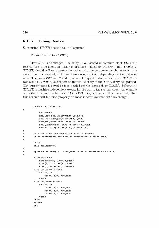
116 PLTMG USERS’ GUIDE 13.0
6.12.2 Timing Routine.
Subroutine TIMER has the calling sequence
Subroutine TIMER( ISW )
Here ISW is an integer. The array TIME stored in common block PLTMG7records the time spent in major subroutines called by PLTMG and TRIGEN.TIMER should call an appropriate system routine to determine the current timeeach time it is entered, and then take various actions depending on the value ofISW. The cases ISW = −2 and ISW = −1 request initialization of the TIME ar-ray, while 1 ≤ ISW ≤ 50 request an individual entry in the TIME array be updated.The current time is saved as it is needed for the next call to TIMER. SubroutineTIMER is machine independent except for the call to the system clock. An exampleof TIMER, calling the function CPU TIME, is given below. It is quite likely thatthis routine will function properly on most modern systems with no change.
subroutine timer(isw)
c
use mthdef
implicit real(kind=rknd) (a-h,o-z)
implicit integer(kind=iknd) (i-n)
integer(kind=iknd), save :: len=50
real(kind=rknd), save :: tx=0.0e0_rknd
common /pltmg7/time(3,50),hist(22,30)
c
c call the clock and return the time in seconds
c (time differences are used to compute the elapsed time)
c
ty=tx
call cpu_time(tx)
c
c update time array (1.0e-10_rknd is below resolution of timer)
c
if(isw>0) then
dt=max(tx-ty,1.0e-10_rknd)
time(1,isw)=time(1,isw)+dt
time(2,isw)=time(2,isw)+dt
else if(isw==-1) then
do i=1,len
time(1,i)=0.0e0_rknd
enddo
else if(isw==-2) then
do i=1,len
time(1,i)=0.0e0_rknd
time(2,i)=0.0e0_rknd
time(3,i)=0.0e0_rknd
enddo
endif
return
end

6.12. Machine Dependent Routines. 117
6.12.3 Command Line Interface
ATEST calls the Fortran subroutine
Subroutine get command( LIST, LENGTH, STATUS )
to obtain a copy of the command line that launched an ATEST application. If thisis not available in the Fortran compiler, one can comment this call, that appearsonly in subroutine ACMD. This disables the dynamic setting of the parametersMODE and WEBPRT but does not affect other aspects of the application.
6.12.4 Graphics Interface.
The four device dependent routines in the graphics package are
Subroutine PLTUTL( NCOLOR, RED, GREEN, BLUE )Subroutine PFRAME( IFRAME )Subroutine PLINE( X, Y, Z, N, ICOLOR )Subroutine PFILL( X, Y, Z, N, ICOLOR )
Subroutine PLTUTL takes various actions depending on the value of the inte-ger NCOLOR. NCOLOR > 0 specifies initialization; NCOLOR denotes the numberof colors to be used and satisfies 2 ≤ NCOLOR ≤ MXCOLR. RED, GREEN ,and BLUE are vectors of length NCOLOR. The entries RED(i), GREEN(i), andBLUE(i), 1 ≤ i ≤ NCOLOR, are floating point numbers on the interval [0, 1],corresponding to rgb values for the ith color. Color number 1 is always white(RED(1) = GREEN(1) = BLUE(1) = 1.0), and color number 2 is always black(RED(2) = GREEN(2) = BLUE(2) = 0.0). The rgb values of the remaining entriesdepend on the picture to be drawn and the value of MXCOLR. PLTUTL shouldcreate a color map with the required colors, as these will be referenced in futurecalls to PLINE and PFILL. If PLTUTL is called with NCOLOR < 0, the drawingis complete and any necessary post processing should be carried out (e.g., close theplot file).
The drawing space used by the graphics routines is always assumed to be eitherthe unit square (0, 1)× (0, 1) or the rectangle (0, 1.5)× (0, 1). For devices that havea so-called Z-buffer, the drawing space is either the unit cube (0, 1)× (0, 1)× (0, 1)or the brick (0, 1.5) × (0, 1) × (0, 1). The graphics display itself is always viewedas rectangular with aspect ratio 3/2, which is either a single rectangular frame orthree square frames. These frames are numbered 1 to 4 as illustrated in Figure 6.5.The graphics routines write their output to various lists. A list consists of a frame,and the attributes rotating/non-rotating. This attribute may not have realizationsfor all graphics devices. The five available lists are summarized in Table 6.4.
When graphics is initiated for a certain list, say list k, subroutine PFRAME(k)is called to indicate that subsequent calls of PLINE and PFILL contain data to bewritten to list k. PFRAME(−k) indicates that the output to the given list shouldbe terminated. By convention, graphics routines are allowed only one open list at

118 PLTMG USERS’ GUIDE 13.0
a time. Therefore, when PFRAME is invoked with a positive argument, the givenlist should be opened and the mapping from the unit cube or brick to the actualdevice coordinates for the given list should be computed. If the rotation attributeis available, it should be set as specified in Table 6.4. When PFRAME is invokedwith a negative argument, the given list should be closed.
1 4
3
2
Figure 6.5. Frame definitions.
list frame rotating
1 1 no2 2 no3 3 no4 4 no5 4 yes
Table 6.4. list specifications for pframe.
Subroutine PLINE has arguments X, Y, Z, N, and ICOLOR. X, Y, and Z arevectors of length N ≥ 2. The points (X(i),Y(i),Z(i)) lie in the unit cube or thebrick (0, 1.5)× (0, 1)× (0, 1). The Z coordinate is useful only for devices that havea Z-buffer, and can be ignored in other cases. ICOLOR is an integer between 1 andNCOLOR, where NCOLOR was the argument that initialized PLTUTL, indicatingthe color to be used. PLINE should draw the given polyline (X(i),Y(i),Z(i)) to(X(i+1),Y(i+1),Z(i+1)), 1 ≤ i ≤ N − 1, with the specified color in the properframe.
Subroutine PFILL has arguments X, Y, Z, N, and ICOLOR. X, Y, and Zare vectors of length N ≥ 3. The points (X(i),Y(i),Z(i)) lie in the unit cube orthe brick (0, 1.5) × (0, 1) × (0, 1), and define an N -sided (planar) polygonal re-gion with sides (X(i),Y(i),Z(i)) to (X(i+1),Y(i+1),Z(i+1)) for 1 ≤ i ≤ N − 1,and (X(N),Y(N),Z(N)) to (X(1),Y(1),Z(1)). ICOLOR is an integer between 1 andNCOLOR, where NCOLOR was the argument that initialized PLTUTL, indicatingthe color to be used. PFILL should color the specified polygon with the specifiedcolor in the proper frame.
The default installation of the PLTMG package includes several output graph-ics devices. These are described in Table 6.5. PostScript and XPM are both ASCIIfiles. The parameter GRFILE specifies the file name. To allow one file name vari-

6.12. Machine Dependent Routines. 119
IDEVCE output device
0 web browser1 XPM file
2 PostScript file
Table 6.5. Default graphics devices.
able to stand for multiple files, the file name GRFILE is scanned for the stringFIGXXX. If it is found, for the first actual file name, it is replaced by FIG001,for the second by FIG002, and so on, allowing each actual file to receive a uniquename. The file name is also scanned for the string .EXT and if found, it is replacedby .XPM or .PS as appropriate. If the string .EXT is not found, the appropriateextension is appended to the existing name. Finally, the file name is scanned for thestring MPIXXX, and if found, the XXX is replaced by the appropriate processornumber.
IPANE WEBGUI canvas graphics type
0 upper right WebGL 3D1 lower left WebGL 3D2 lower right WebGL 3D3 upper right Pixmap 2D4 lower left Pixmap 2D5 lower right Pixmap 2D
Table 6.6. IPANE definitions.
The web browser interface provides both 2D and 3D graphics. The canvasand the type of graphics are specified through the parameter IPANE, as describedin Table 6.6. The parameters FPANE, JPANE, and GPANE are associated withgraphics subroutines TRIPLT, INPLT, and GPHPLT, respectively, and specify thevalue of IPANE to be used with that routine.
WebGL graphics written to LIST = 5 can be manipulated with the mouse.Mouse button one (left) can be used to rotate the image. Button two (middle) isused to pan the image, and button three (right) can be used to zoom. On Applesystems with a one button mouse, buttons two and three are simulated by pressingthe OPTION and COMMAND keys, respectively, simultaneously with the mouse.In WebGL windows, the OPTION + I toggle referenced in Table 6.2 can displaythe numerical values for the zoom, rotation matrix and translation.
Additionally, associated with each WebGL canvas are seven buttons. Theseare described in Table 6.7.
The RESET button returns the image to its initial state, removing any pan,zoom and rotation operations that the user may have applied. OPTION + R

120 PLTMG USERS’ GUIDE 13.0
button effect
RESET return a zoomed/panned/rotated image to its initial stateFREE clear the image and free associated memorySPIN spin imagePOP place canvas in its own web browser tabPUSH return canvas to its original location in the web browser tabSAVE save image to a fileLOAD read image from a file
Table 6.7. WebGL graphics window buttons.
toggles between automatically invoking the RESET button each time a new imageis displayed, and retaining the pan, zoom and rotate position of the previous image.
When the POP button is pushed, the graphics window is removed from thearray of graphics windows in the main web browser display, and appears in a sep-arate tab. This is useful, as typically the size of the image increases. In the newtab, the POP button is replaced by one labeled PUSH. When the PUSH button ispressed, the canvas is returned to its previous location in the main display. TheSAVE button saves a binary file containing the image, which can later be restoredusing the LOAD button. If the OPTION key is pressed simultaneously with theSAVE button as indicated in Table 6.2, then the image is saved as an ASCII file.
If 3 ≤ IPANE ≤ 5 then only the FREE button appears. These values ofIPANE are useful to preview pixmaps, that can then later be saved as XPM files.
6.12.5 MPI Interface
The communication used in parallel processing is provided by calls to the MPIlibrary. This library is not provided as part of the PLTMG package. The calls tothe MPI library are all made from Fortran, and we have concentrated all calls intojust a few subroutines. Thus the vast majority of the code comprising the mainPLTMG routines is self-contained. If the MPI library is not available, one can usesubstitute stub routines supplied with the default installation in place of the regularinterface. The stub routines are similar to the those in the regular interface, exceptthat all calls to routines and functions in the MPI library have been deleted. Usingthe stub routines, an executable can be created without the need to load the MPIlibrary to resolve external references. In this case, all the parallel computing optionsprovided by PLTMG, TRIGEN, and the graphics routines are disabled.

Chapter 7
Test Problems
7.1 Overview.In this chapter, we briefly document the test problem data sets included with thePLTMG source code. These problems encompass a variety of applications andexercise most features of the package. Each data set minimally consists of functionsA1XY, A2XY, FXY, GNXY, GDXY, P1XY, P2XY, and QXY and subroutinesUSRCMD and GDATA. Problem specific routines are also included.
7.2 Test Problem CIRCLE.In this problem, we solve the equation
−∇ · (a∇u) = 0,
where Ω is the unit circle with a crack along the positive x axis. HomogeneousDirichlet boundary conditions are imposed on the top of the crack, and homogeneousNeumann boundary conditions are imposed below the crack. The coefficient a ≡ akis piecewise constant in the eight sectors
Ωk = (r, θ)| 0 ≤ r ≤ 1, (k − 1)π/4 ≤ θ ≤ kπ/4.
The domain Ω is defined by a triangulation consisting of eight similar triangles,shown in Figure 7.1, that correspond to the eight sectors of constant a. On theboundary of the circle, nonhomogeneous boundary conditions are imposed suchthat the true solution in sector Ωk is given by
u = rα(βk sinαθ + γk cosαθ). (7.1)
The exponent α is chosen to correspond to the leading singularity arising fromthe geometry, change of boundary conditions, and coefficient jumps at the origin.The coefficients βk and γk are chosen to insure continuity of the solution u andthe normal component of the flux a∇u · n across the interfaces, and to satisfy the
121

122 PLTMG USERS’ GUIDE 13.0
boundary conditions along the crack. For example, in the case ak = 1 for all k,α = 1/4 and
u = rα sinαθ.
The USRCMD for this test problem has ten parameters that can be set. IBCdetermines the boundary conditions. If IBC = 2, the boundary conditions on theouter boundary of the circle are nonhomogeneous Dirichlet chosen such that (7.1)is the exact solution; if IBC = 1, nonhomogeneous Neumann boundary conditionsare imposed on the circular part of the boundary in a similar fashion. One can alsoalter the geometry of the domain using the parameter NTRI, where 1 ≤ NTRI ≤ 8.If NTRI = 8 the entire circle is used as the domain; if NTRI < 8, only the firstNTRI sectors are used. Some examples are shown in Figure 7.1. Eight parameters,
Figure 7.1. On the far right is the square domain for problems SQUARE,OB and CONTROL. The remaining domains are for test problem CIRCLE withNTRI = 8, NTRI = 7 and NTRI = 3.
A1, A2,. . . ,A8 define the coefficients ak. Given the ak and NTRI, the values ofα, βk and γk are computed in GDATA by solving appropriate nonlinear equations.Since the exact solution is known, we can compute the exact error. For this testproblem, the function QXY is defined to be the exact error for graphics optionsand the true solution (7.1) otherwise.
7.3 Test Problem SQUARE.In this test problem, a complicated equation is solved on a simple domain. Thedomain is always the unit square shown in Figure 7.1; boundary conditions on eachside of the square can be independently specified as Dirichlet or natural, or pairs ofopposite sides can be specified as periodic. The region is specified as a triangulation.
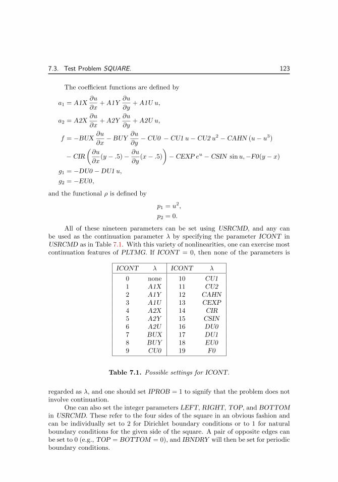
7.3. Test Problem SQUARE. 123
The coefficient functions are defined by
a1 = A1X∂u
∂x+ A1Y
∂u
∂y+ A1U u,
a2 = A2X∂u
∂x+ A2Y
∂u
∂y+ A2U u,
f = −BUX∂u
∂x− BUY
∂u
∂y− CU0 − CU1 u− CU2 u2 − CAHN (u− u3)
− CIR
(∂u
∂x(y − .5)− ∂u
∂y(x− .5)
)− CEXP eu − CSIN sinu,−F0(y − x)
g1 = −DU0 −DU1 u,
g2 = −EU0,
and the functional ρ is defined by
p1 = u2,
p2 = 0.
All of these nineteen parameters can be set using USRCMD, and any canbe used as the continuation parameter λ by specifying the parameter ICONT inUSRCMD as in Table 7.1. With this variety of nonlinearities, one can exercise mostcontinuation features of PLTMG. If ICONT = 0, then none of the parameters is
ICONT λ ICONT λ
0 none 10 CU11 A1X 11 CU22 A1Y 12 CAHN3 A1U 13 CEXP4 A2X 14 CIR5 A2Y 15 CSIN6 A2U 16 DU07 BUX 17 DU18 BUY 18 EU09 CU0 19 F0
Table 7.1. Possible settings for ICONT.
regarded as λ, and one should set IPROB = 1 to signify that the problem does notinvolve continuation.
One can also set the integer parameters LEFT, RIGHT, TOP, and BOTTOMin USRCMD. These refer to the four sides of the square in an obvious fashion andcan be individually set to 2 for Dirichlet boundary conditions or to 1 for naturalboundary conditions for the given side of the square. A pair of opposite edges canbe set to 0 (e.g., TOP = BOTTOM = 0), and IBNDRY will then be set for periodicboundary conditions.

124 PLTMG USERS’ GUIDE 13.0
7.4 Test Problem DOMAINS.In this test problem, a simple equation is solved on a variety of complicated domains.This test problem was designed mainly to exercise TRIGEN.
The problem to be solved is the linear partial differential equation
a1 = A1X∂u
∂x+ A1Y
∂u
∂y+ A1U u,
a2 = A2X∂u
∂x+ A2Y
∂u
∂y+ A2U u,
f = −BUX∂u
∂x− BUY
∂u
∂y− CU1 u− CU0
with a combination of homogeneous Dirichlet, homogeneous Neumann, and peri-odic boundary conditions. The parameters A1X, A1Y, A1U, A2X, A2Y, A2U,BUX, BUY, CU0, and CU1 can all be set in USRCMD. The parameter DOMAIN,satisfying 1 ≤ DOMAIN ≤ 21, specifies the domain to be used. The various possi-bilities are shown in Figure 7.2. All domains are defined by skeletons, so TRIGENmust be called to generate a triangulation.
7.5 Test Problem NACA.Test problem NACA solves the equation in one of several domains. The equationis of the form
−∇ · (θρ(∇u) + (1− θ))∇u = 0,
whereρ(∇u) = (1− u2
x − u2y)
1γ−1
and γ = 1.4. When θ = 1, this is the equation of potental flow, and θ = 0corresponds to the Laplace equation. The local Mach number is computed in QXYand is given by
q =
√2c
γ − 1,
c =1
1− u2x − u2
y
− 1.
There are four domain options, chosen using the parameter DOMAIN in USR-CMD. These domains are shown in Figure 7.3. All regions are defined as skeletons,so TRIGEN must be used to generate a triangulation.
Neumann boundary conditions are imposed everywhere so each domain hasISING = 1. There are several parameters in USRCMD that affect these problems.The parameter MINF, specifying the Mach number at infinity M∞, sets the bound-ary conditions on the outer boundary. The parameter ANGLE specifies the angle ofattack (in degrees). The parameter SIZE sets the radius of the outer boundary. Theparameter THETA sets the value of θ defined above. When the local Mach numberis less than one the flow is subsonic; PLTMG will work well in regions where the

7.5. Test Problem NACA. 125
Figure 7.2. The domains for DOMAIN = i, 1 ≤ i ≤ 23.

126 PLTMG USERS’ GUIDE 13.0
Figure 7.3. The domains for DOMAIN = i, 1 ≤ i ≤ 4, with SIZE = 1.
flow is entirely subsonic. As the M∞ is increased, the solution will begin to developregions of supersonic flow near the airfoils; PLTMG will continue to work as theseregions are forming, but eventually will fail, as the underlying discretization usedby PLTMG is not really appropriate for hyperbolic problems.
7.6 Test Problem JCN.Test problem JCN solves the convection diffusion equation
−∇ · (∇u+ βu) = 0,
where β is piecewise constant. The region is shown in Figure 7.4. The domain isspecified by skeleton, so TRIGEN must be used to generate a triangulation.
Figure 7.4. The domain for test problem JCN (left), a triangulation pro-duced by TRIGEN (middle), and the corresponding triangulation after a call toUSRCMD with OBTUSE = 1 (right).
This problem is an idealized model of the current continuity equation from thesemiconductor device model that we have used to study the stability of discretiza-tions used in device simulation. The problem has seven regions; β = 0 in regionsone and seven. In the other five regions it has a magnitude of approximately 104
and is directed radially in each of the five subregions. The solution develops steepgradients at the junction between region seven and the five adjoining subregions.
Constant nonhomogeneous Dirichlet boundary conditions are specified alongthe bottom of the domain and on the left-hand portion of the top of the domain.Homogeneous Neumann boundary conditions are imposed elsewhere. The parame-ters TOP and BOTTOM in USRCMD can be used to reset the Dirichlet boundary

7.7. Test Problem OB. 127
conditions on the top and bottom of the domain. The parameter DU can be usedto adjust the size of β in regions 2–5; in particular, the magnitude of β in these fiveregions is proportional to DU.
Our original purpose in constructing this example was to test the sensitivity ofvarious upwinding techniques [7] to poor element geometries. Since the goal of TRI-GEN is to produce elements with good geometries, the USRCMD for this problemincludes a procedure for systematically degrading the quality of the triangulation byintroducing new elements with obtuse angles. If OBTUSE = 1 in USRCMD, theneach triangle in the current mesh is divided into three new triangles by connectingits barycenter to its vertices. An example is shown in Figure 7.4. Repeated appli-cation of this procedure will produce triangulations with interior angles arbitrarilyclose to π.
7.7 Test Problem OB.Test problem OB solves the a simple obstacle problem, with coefficient functionsdefined by
p1 = AX
(∂u
∂x
)2
+ AY
(∂u
∂y
)2
+ CU u2 − 2su,
s =(AX(IXπ)2 + AY (IYπ)2 − CU
)sin(IXπx) sin(IYπy),
u = BDLW + CFLW sin(IXLπx) sin(IYLπy),
u = BDUP + CFUP sin(IXUπx) sin(IYUπy),
g1 = 0.
The domain Ω is the unit square with homogeneous Dirichlet boundary condi-tions. The input data structure is a triangulation consisting of eight right trian-gles, shown in Figure 7.1. The parameters AX, AY, CU, BDLW, BDUP, CFLW,CFUP and the integers IX, IY, IXL, IYL, IXU, IYU can all be set by the userin USRCMD. The exact solution to this problem in the absence of the obstacleis u = sin(IXπx) sin(IYπy). This problem is mainly designed to test the casesIPROB = ±2 in PLTMG.

128 PLTMG USERS’ GUIDE 13.0
7.8 Test Problem MNSURF.Test problem MNSURF solves the a simple minimal surface problem with an ob-stacle. The coefficient functions are given by
p1 =
√1 +
(∂u
∂x
)2
+
(∂u
∂y
)2
u =
1 in Ω1
−1 in Ω2
` in ΩI
u = 1.5
g1 = 0,
g2 = 0.
The domain Ω is the unit square with a mixture of homogeneous Dirichlet andNeumann boundary conditions. The domain is given as a skeleton, and is shownin Figure 7.5. The region Ω1 is the inner square with side 1/2, and Ω2 is the outerregion. The region ΩI is the small band separating Ω1 and Ω2, consisting of fournarrow trapezoids. In each of the four trapezoids, u is a linear polynomial in xor y that interpolates between −1 and 1, insuring continuity of u. The parameterTHETA, which can be set in USRCMD, controls the width of the band. The upperbound u is chosen such that it does not affect the solution. As with test problemOB, this problem is mainly designed to test the cases IPROB = ±2 in PLTMG.
Figure 7.5. The domains for test problems MNSURF, BATTERY,IDENT, and BURGER (left to right).
7.9 Test Problem BURGER.Test problem BURGER solves the nonlinear convection dominated flow
−ε∆u+ uy + uux = 0.
This is really a time dependent Burger’s equation in one space dimension. In thissetting, the y space variable plays the role of time, and we have added a small diffu-sion term. This problem is solved as a two dimensional steady state problem. Some

7.10. Test Problem BATTERY. 129
analysis of this approach to solving time dependent partial differential equations isgiven in [34].
The small parameter ε > 0 and can be set in USRCMD. The domain Ω isthe quarter circle shown in Figure 7.5, and is specified as a skeleton. Natural(homogeneous Neumann) boundary conditions are applied along the circular arc,while Dirichlet boundary conditions are specified on the left side (x = 0) and thebottom (y = 0) as
g2 =
1 0 ≤ x ≤ 1/43/2− 2x 1/4 ≤ x ≤ 3/4
0 3/4 ≤ x ≤ 2.
This combination of boundary conditions gives rise to a solution similar to theso-called “λ shock” of Burger’s equation.
7.10 Test Problem BATTERY.In this test problem we solve the linear elliptic problem
−a1uxx − a2uyy − f = 0
where the piecewise constant values of the coefficients are given in Table 7.2. The
Region a1 a2 f side c α
1 25 25 0 left 0 02 7 0.8 1 top 1 33 5.0 10−4 1 right 2 24 0.2 0.2 0 bottom 3 15 0.05 0.05 0
Table 7.2. Coefficient definitions.
domain Ω is shown in Figure 7.5 and is specified as a skeleton. The five subregionsare given labels in ITNODE(5,*), allowing us to conveniently define the coefficientfunctions. The boundary conditions are natural boundary conditions of the form
g1 = c− αu.
Here c and α are piecewise constant functions defined using IBNDRY(6,*), as indi-cated in Table 7.2. The data for this problem was supplied by Leszek Demkowicz.
7.11 Test Problem CONTROL.This problem tests the cases IPROB = ±5. The differential equation (constraint)is
−∆u = λ(C0 + C1u+ C2u2 + C3u3) + F0 + F1u+ F2u2 + F3u3

130 PLTMG USERS’ GUIDE 13.0
in Ω, with Dirichlet boundary conditions
u = DBC
on ∂Ω. The objective function ρ is given by
ρ(u, λ) =
∫Ω
(u− u0)2 + β|∇(u− u0)|2 + γλ2 dx.
Ω is the unit square, defined as a triangulation similar to test problem SQUARE;see Figure 7.1. The function u0 and the bounds on λ are given by
u0 = sin(IXπx) sin(IYπy),
BDLW ≤ λ ≤ BDUP.
The constants BETA = β. GAMMA = γ, BDLW, BDUP, DBC, C0, C1, C2, C3,F0, F1, F2, and F3, and the integers IX and IY can all be reset in USRCMD.
7.12 Test Problem IDENT.This problem tests the cases IPROB = ±4. The differential equation is
−(1 + A2)∆u+ C2 u2 + C1 u− C0 = 0.
The domain Ω is specified as a skeleton, and is shown in Figure 7.5. The boundaryconditions are a combination of homogeneous Neumann and Dirichlet, except for thevertical edge on the right where the (possibly) nonhomogeneous Dirichlet boundarycondition
u = D
is imposed. The five parameters A, C0, C1, C2, and D can be set in USRCMD, andany combination of them can be used as scalar parameters λi in the optimizationproblem. This is done setting the switches IRL (also set in USRCMD) indicatedin Table 7.3. For example, setting IRL1 = 1 makes A an optimization parameter,while setting IRL1 = 0 keeps A at its current fixed value.
switch λj
IRL1 AIRL2 C0IRL3 C1IRL4 C2IRL5 D
Table 7.3. IRL switches.
The objective function ρ is given by
ρ(u, λ) =
∫Ω
e−20(x2+y2)(u− 1)2 dx,
which tries to make the solution u = 1 near the origin, located at the center of Ω.

7.13. Test Problem BOX. 131
7.13 Test Problem BOX.Test problem BOX tests the moving boundary optimization option in PLTMG(IPROB = 4 and ITASK = 8). The domain is a 1 × 1 square with a square hole,illustrated in Figure 7.6. The hole is free to move around within the square, withits position governed by three parameters: (xc, yc) denoting the coordinates of thecenter of the square, and θ denoting its angle of rotation. Any combination ofthese three parameters may be chosen as optimization parameters, as summarizedin Table 7.4.
switch λj
IRL1 xcIRL2 ycIRL3 θ
Table 7.4. IRL switches.
The objective function is given by
ρ(u, λ) = min
∫Ω
∇u2 + δ
NRL∑i=1
λ2i dx.
The boundary value problem and inequality constraints are given by
−∆u = 1 in Ω
u = 0 on ∂Ω
λi ≤ λi ≤ λi, for 1 ≤ i ≤ NRL.
7.14 Test Problem MESSAGE.In this test problem, a simple equation is solved on a domain consisting of a messagewith up to ten lines. This test problem was designed mainly for fun, and to makesoftware demonstrations more interesting.
The problem to be solved is the linear partial differential equation
a1 = A1X∂u
∂x+ A1Y
∂u
∂y+ A1U u,
a2 = A2X∂u
∂x+ A2Y
∂u
∂y+ A2U u,
f = −BUX∂u
∂x− BUY
∂u
∂y− CU1 u− CU0
with homogeneous Dirichlet boundary conditions. The parameters A1X, A1Y, A1U,A2X, A2Y, A2U, BUX, BUY, CU0, and CU1 can all be set in USRCMD. String

132 PLTMG USERS’ GUIDE 13.0
parameters LINE0, LINE1, ... , LINE9 can be set in USRCMD to a user specifiedmessage. Upper case and lower case letters, numbers, and several symbols found ona standard keyboard are available. Two possible domains are shown in Figure 7.6.All domains are defined by skeletons, so TRIGEN must be called to generate atriangulation.
Figure 7.6. The domain for test problem BOX, and two sample domainsfor test problem MESSAGE.
7.15 Test Problem USMAP.In this test problem, a simple equation is solved on one of 51 domains; 50 areoutlines of individual states in the United States, and the last is an outline of thecontinental U. S. As with test problem MESSAGE, this test problem was designedmainly for fun.
The problem to be solved is the linear partial differential equation
a1 = A1X∂u
∂x+ A1Y
∂u
∂y+ A1U u,
a2 = A2X∂u
∂x+ A2Y
∂u
∂y+ A2U u,
f = −BUX∂u
∂x− BUY
∂u
∂y− CU1 u− CU0
with homogeneous Dirichlet boundary conditions. The parameters A1X, A1Y, A1U,A2X, A2Y, A2U, BUX, BUY, CU0, and CU1 can all be set in USRCMD.
All domains are specified as skeletons, derived from PostScript and PDF filesfrom the National Digital Map Library at the University of Virginia. The parameterISTATE, 1 ≤ ISTATE ≤ 51, specifies the domain. The parameter ICTY takes onvalues 0 and 1; if ICTY = 1, county lines (state lines in the case of the U. S. map)are included as part of the skeleton. If ICTY = 0, the skeleton consists of just theoutline of the state or country. Several domains (e. g. Michigan, Hawaii) are notconnected. Many have small islands11 that can be excluded from the skeleton bysetting the parameter ISLE = 0. If ISLE = 1, all small islands are included as partof the skeleton. Several domains are shown in Figure 7.7. Since all domains aredefined by skeletons, TRIGEN must be called to generate a triangulation.
11The definition of small is problem dependent and depends on the judgment of the author.

7.15. Test Problem USMAP. 133
Figure 7.7. Sample domains for test problem USMAP. ICNTY = 1 andISLE = 0 for all domains.

134 PLTMG USERS’ GUIDE 13.0

Bibliography
[1] I. Babuska and W. C. Rheinboldt, Error estimates for adaptive finiteelement computations, SIAM J. Numer. Anal., 15 (1978), pp. 736–754.
[2] Ivo Babuska and Theofanis Strouboulis, The finite element method andits reliability, Numerical Mathematics and Scientific Computation, The Claren-don Press Oxford University Press, New York, 2001.
[3] Randolph E. Bank, A domain decomposition solver for a parallel adaptivemeshing paradigm, in Domain Decomposition Methods in Science and Engi-neering XVI, Olof B. Widlund and David E. Keyes, eds., vol. 55 of LectureNotes in Computational Science and Engineering, Springer-Verlag, 2006, pp. 3–14.
[4] , Some variants of the Bank-Holst parallel adaptive meshing paradigm,Computing and Visualization in Science, 9 (2006), pp. 133–144.
[5] , Multigraph users’ guide - version 2.0, tech. report, Department of Math-ematics, University of California at San Diego, 2015.
[6] , A two level solver for hp adaptive finite element equations, Computingand Visualization in Science, (to appear).
[7] R. E. Bank, J. F. Burgler, W. Fichtner, and R. K. Smith, Someupwinding techniques for finite element approximations of convection-diffusionequations, Numer. Math., 58 (1990), pp. 185–202.
[8] Randolph E. Bank and Tony F. Chan, PLTMGC: A multi-grid continu-ation program for parameterized nonlinear elliptic systems, SIAM J. Sci. andStat. Computing, 7 (1986), pp. 540–559.
[9] , An analysis of the composite step biconjugate gradient method, Numer.Math., 66 (1993), pp. 295–319.
[10] , The composite step biconjugate gradient algorithm for nonsymmetriclinear systems, Numerical Algorithms, 7 (1994), pp. 1–16.
[11] Randolph E. Bank, William M. Coughran, and Lawrence C.Cowsar, Analysis of the finite volume Scharfetter-Gummel method for steady
135

136 Bibliography
convection diffusion equations, Computing and Visualization in Science, 1(1998), pp. 123–136.
[12] Randolph E. Bank and Chris Deotte, Adventures in adaptivity, Com-puting and Visualization in Science, 18 (2017), pp. 79–82.
[13] , The influence of partitioning on domain decomposition convergencerates, Computing and Visualization in Science, 18 (2017), pp. 53–64.
[14] Randolph E. Bank, Philip E. Gill, and Roummel F. Marcia, In-terior methods for a class of elliptic variational inequalities, in Large-scalePDE-constrained Optimization, Lorenz T. Biegler, Omar Ghattas, MatthiasHeinkenschloss, and Bart van Bloemen Waanders, eds., vol. 30 of Lecture Notesin Computational Science and Engineering, Berlin, Heidelberg and New York,2003, Springer-Verlag, pp. 218–235.
[15] Randolph E. Bank and Michael J. Holst, A new paradigm for paralleladaptive meshing algorithms, SIAM J. on Scientific Computing, 22 (2000),pp. 1411–1443.
[16] , A new paradigm for parallel adaptive meshing algorithms, SIAM Review,45 (2003), pp. 292–323.
[17] Randolph E. Bank and Peter K. Jimack, A new parallel domain decom-position method for the adaptive finite element solution of elliptic partial dif-ferential equations, Concurrency and Computation: Practice and Experience,13 (2001), pp. 327–350.
[18] Randolph E. Bank, Peter K. Jimack, Sarfraz A. Nadeem, andSergei V. Nepomnyaschikh, A weakly overlapping domain decompositionpreconditioner for the finite element solution of elliptic partial differential equa-tions, SIAM J. on Scientific Computing, 23 (2002), pp. 1817–1841.
[19] Randolph E. Bank and Shaoying Lu, A domain decomposition solver fora parallel adaptive meshing paradigm, SIAM J. on Scientific Computing, 45(2003), pp. 292–323.
[20] Randolph E. Bank and Hans D. Mittelmann, Continuation and multi-grid for nonlinear elliptic systems, in Multigrid Methods II: Proceedings,Cologne 1985, vol. 1228 of Lecture Notes in Mathematics, Springer-Verlag,Heidelberg, 1986, pp. 24–38.
[21] , Stepsize selection in continuation procedures and damped Newton’smethod, J. Comput. Appl. Math., 26 (1989), pp. 67–78.
[22] Randolph E. Bank and Hieu Nguyen, Domain decomposition and hp-adaptive finite elements, in Domain Decomposition Methods in Science andEngineering XIX, Yunqing Huang, Ralf Kornhuber, Olof Widlund, and JinchaoXu, eds., vol. 78 of Lecture Notes in Computational Science and Engineering,Springer-Verlag, 2011, pp. 3–13.

Bibliography 137
[23] , hp adaptive finite elements based on derivative recovery and supercon-vergence, Computing and Visualization in Science, 14 (2012), pp. 287–299.Original Article.
[24] , Mesh regularization in the Bank-Holst parallel hp adaptive meshing, inDomain Decomposition Methods in Science and Engineering XX, RandolphBank, Michael Holst, Olof Widlund, and Jinchao Xu, eds., vol. 91 of Lec-ture Notes in Computational Science and Engineering, Springer-Verlag, 2013,pp. 103–110.
[25] , A parallel hp-adaptive finite element method, in Scientific Computingand Applications VIII, Jichun Li, ed., vol. 586 of Contemporary Mathematics,American Mathematical Society, 2013, pp. 23–33.
[26] Randolph E. Bank and Jeffery S. Ovall, Dual functions for a paralleladaptive method, SIAM J. on Scientific Computing, 29 (2007), pp. 1511–1524.
[27] , Some remarks on interpolation and best approximation, NumerischeMathematik, (accepted).
[28] Randolph E. Bank, Aseih Parsania, and Stefan Sauter, Saturation es-timates for hp-finite element mathods, Computing and Visualization in Science,16 (2013), pp. 195–218.
[29] Randolph E. Bank and Donald J. Rose, Global approximate Newtonmethods, Numer. Math., 37 (1981), pp. 279–295.
[30] , A multi-level Newton method for nonlinear finite element equations,Math. Comp., 39 (1982), pp. 453–465.
[31] Randolph E. Bank and R. Kent Smith, Mesh smoothing using a posteriorierror estimates, SIAM J. Numer. Anal., 34 (1997), pp. 979–997.
[32] Randolph E. Bank and R. Kent Smith, Multigraph algorithms based onsparse Gaussian elimination, in Thirteenth International Symposium on Do-main Decomposition Methods for Partial Differential Equations, Domain De-composition Press, Bergen, 2001, pp. 15–26.
[33] , An algebraic multilevel multigraph algorithm, SIAM J. on Scientific Com-puting, 25 (2002), pp. 1572–1592.
[34] Randolph E. Bank, Panayot Vassilevski, and Ludmil Zikatanov, Ar-bitrary dimension convection-diffusion scheme for sapce-time discretizations,Journal of Computational and Applied Mathematics, (accepted).
[35] Randolph E. Bank and Panayot S. Vassilevski, Convergence analysisof a domain decomposition paradigm, Computing and Visualization in Science,11 (2008), pp. 333–350.
138 Bibliography
[36] Randolph E. Bank and Jinchao Xu, Asymptotically exact a posteriori er-ror estimators, part I: Grids with superconvergence, SIAM J. Numerical Anal-ysis, 41 (2003), pp. 2294–2312.
[37] , Asymptotically exact a posteriori error estimators, part II: General un-structured grids, SIAM J. Numerical Analysis, 41 (2003), pp. 2313–2332.
[38] Randolph E. Bank, Jinchao Xu, and Bin Zheng, Superconvergent deriva-tive recovery for Lagrange triangular elements of degree p on unstructured grids,SIAM J. Numerical Analysis, 45 (2007), pp. 2032–2046.
[39] Randolph E. Bank and Harry Yserentant, On the H1-stability of theL2-projection onto finite element spaces, Numerische Mathematik, 126 (2014),pp. 361–381.
[40] , A note on interpolation, best approximation, and the saturation property,Numerische Mathematik, 131 (2015), pp. 199–203.
[41] , On the convergence of adaptive feedback loops, Numerische Mathematik,(submitted).
[42] Mark W. Beall and Mark S. Shephard, A general topology-based meshdata structure, Internat. J. Numer. Methods Engrg., 40 (1997), pp. 1573–1596.
[43] X. Cai and K. Samuelsson, Parallel multilevel methods with adaptivity onunstructured grids, 1999. Preprint.
[44] T. F. Chan, P. Ciarlet, and W. K. Szeto, On the optimality of the mediancut spectral bisection method, SIAM J. Sci. Comput., 18 (1997), pp. 943–948.
[45] H. L. deCougny, K. D. Devine, J. E. Flaherty, R. M. Loy, C. Oztu-ran, and M. S. Shephard, Load balancing for the parallel adaptive solutionof partial differential equations, Appl. Num. Math., 16 (1994), pp. 157–182.
[46] C. Deotte, Domain Partitioning Methods for Elpiptic Partial DifferentialEquations, PhD thesis, University of California at San Diego, 2014.
[47] Christopher Deotte, Webgui: A web browswer based graphical user inter-face for scientific software users’ guide, tech. report, Department of Mathe-matics, University of California at San Diego, 2017.
[48] J. E. Flaherty, R. M. Loy, C. Ozturan, M. S. Shephard, B. K. Szy-manski, J. D. Teresco, and L. H. Ziantz, Parallel structures and dynamicload balancing for adaptive finite element computation, Appl. Num. Math., 26(1998), pp. 241–263.
[49] Andrew V. Knyazev, Toward the optimal preconditioned eigensolver: locallyoptimal block preconditioned conjugate gradient method, SIAM J. Sci. Comput.,23 (2001), pp. 517–541 (electronic). Copper Mountain Conference (2000).

Bibliography 139
[50] Scott Kohn, John Weare, M. Elizabeth Ong, and Scott B. Baden,Software abstractions and computational issues in parallel structured adaptivemesh methods for electronic structure calculations, in Workshop on StructuredAdaptive Mesh Refinement Grid Methods, Institute for Mathematics and ItsApplications, University of Minnesota, Minneapolis, MN., 1997.
[51] Shaoying Lu, Parallel Adaptive Multigrid Algorithms, PhD thesis, Depart-ment of Mathematics, University of California at San Diego, 2004.
[52] William F. Mitchell, A comparison of adaptive refinement techniques forelliptic problems, ACM Trans. Math. Software, 15 (1989), pp. 326–347.
[53] , The full domain partition approach to distributing adaptive grids, Ap-plied Numerical Mathematics, 26 (1998), pp. 265–275.
[54] , A parallel multigrid method using the full domain partition, ElectronicTransactions on Numerical Analysis, 6 (1998), pp. 224–233.
[55] Hans D. Mittelmann, Multi-grid continuation and spurious solutions fornonlinear boundary value problems, Rocky Mountain J. Math., 18 (1988),pp. 387–401.
[56] H. D. Mittelmann and H. Weber, Multigrid solution of bifurcation prob-lems, SIAM J. Sci. Stat. Comp., 6 (1985), pp. 49–60.
[57] Hieu Nguyen, p- and fully automatic hp- adaptive finite element methods forelliptic Partial Differential Equations, PhD thesis, University of California, SanDiego, 2010.
[58] Jeffrey S. Ovall, Duality-Based Adaptive Refinement for Elliptic PDEs,PhD thesis, Department of Mathematics, University of California at San Diego,2004.
[59] B. N. Parlett, The Symmetric Eigenvalue Problem, Prentice Hall, Engle-wood Cliffs, New Jersey, 1980.
[60] Alex Pothen, Horst D. Simon, and Kang-Pu Liou, Partitioning sparsematrices with eigenvectors of graphs, SIAM J. Matrix Anal. Appl., 11 (1990),pp. 430–452.
[61] M. C. Rivara, Mesh refinement processes based on the generalized bisectionof simplices, SIAM J. Numer. Anal., 21 (1984), pp. 604–613.
[62] P. M. Selwood, M. Berzins, and P. M. Dew, 3D parallel mesh adaptivity:Data structures and algorithms, in Parallel Processing for Scientific Computing,Philadelphia, 1997, SIAM.
[63] Horst D. Simon and Shang-Hua Teng, How good is recursive bisection?,SIAM J. Sci. Comput., 18 (1997), pp. 1436–1445.

140 Bibliography
[64] Rudiger Verfurth, A Posteriori Error Estimation and Adaptive Mesh Re-finement Techniques, Teubner Skripten zur Numerik, B. G. Teubner, Stuttgart,1995.
[65] C. Walshaw and M. Berzins, Dynamic load balancing for pde solvers onadaptive unstructured meshes, Concurrency: Practice and Experience, 7 (1995),pp. 17–28.
[66] A. Weiser, Local-Mesh, Local-Order Adaptive Finite Element Methods withA-Posteriori Error Estimators for Elliptic Partial Differential Equations, PhDthesis, Yale University, 1981.
[67] Linbo Zhang, Tao Cui, and Hui Liu, A set of symmetric quadrature ruleson triangles and tetrahedra, J. Comput. Math., 27 (2009), pp. 89–96.
Index
A1XYcalling sequence, 28
A2XYcalling sequence, 28
ANGMN, see Table 2.13ANORM, see Table 2.13AREA, see Table 2.13ATEST
array dimensions, 111commands, 102common blocks, 111initialization defaults, 111reading data files, 112resetting parameters
long form, 103short form, 104
writing data files, 112ATEST1
common block, 111ATEST2
common block, 111ATEST3
common block, 111ATEST4
common block, 111ATEST5
common block, 111ATEST6
common block, 111ATEST7
common block, 111
BEST, see Table 2.13BFILE, see Table 2.14
PLTMG output, 73definition, 101
BLUE
definition, 117BMNRM0, see Table 2.13BNORM
definition, 72BNORM0, see Table 2.13BRATIO, see Table 2.13
calling sequenceA1XY, 28A2XY, 28CENTRE, 11FXY, 28GDATA, 114GDXY, 31GNXY, 31GPHPLT, 94INPLT, 91P1XY, 28P2XY, 31PFILL, 117PFRAME, 117PLINE, 117PLTMG, 59PLTUTL, 117QXY, 32SKLUTL, 18SXY, 12TIMER, 116TRIGEN, 37TRIPLT, 84USRCMD, 112USRFIL, 113USRSET, 113
CENTREcalling sequence, 11
CENX, see Table 2.13definition, 88, 93
141

142 Index
CENY, see Table 2.13definition, 88, 93
CMD, see Table 2.14coefficient functions, 28common block
ATEST1, 111ATEST2, 111ATEST3, 111ATEST4, 111ATEST5, 111ATEST6, 111ATEST7, 111PLTMG1, 28PLTMG2, 28PLTMG3, 28PLTMG4, 28PLTMG5, 28PLTMG6, 28PLTMG7, 28VAL0, 30VAL1, 31VAL2, 32VAL3, 32VAL4, 12
curved edgescircular arcs, 10parametric, 11
DELTA, see Table 2.13definition, 72
DIAM, see Table 2.13DNEW, see Table 2.13DRDRL, see Table 2.13
definition, 68DTOL, see Table 2.13
definition, 62, 64
Edefinition, 19, 21, 43
E0, see Table 2.13EAVE2, see Table 2.13
definition, 44EF, see Table 2.13eigenvalue problem, 73element quality, 38ENORM1, see Table 2.13
definition, 42ENORM2, see Table 2.13
definition, 42
f command, see Table 6.1IDEVCE, see Table 2.12FPANE, 119FTITLE, see Table 2.14
definition, 84FXY
calling sequence, 28
g command, see Table 6.1GDATA
calling sequence, 114FPANE, see Table 2.12GPANE, see Table 2.12JPANE, see Table 2.12GDXY
calling sequence, 31GET COMMAND
calling sequence, 117GF, see Table 2.9
definition, 19GNXY
calling sequence, 31GPANE, 119GPHPLT
calling sequence, 94continuation path, 98error estimates, 98multigraph convergence histories,
96Newton convergence history, 94timing statistics, 97
GRADE, see Table 2.13definition, 39
GREENdefinition, 117
GRFILEdefinition, 118
GTITLE, see Table 2.14definition, 94
HMAX, see Table 2.13definition, 39

Index 143
HMIN, see Table 2.13
i command, see Table 6.1IADAPT, see Tables 2.12 and 3.1
definition, 37IBNDRY, see also Table 2.1
definition, 15ICONT, see Table 2.12, see Table 5.2
definition, 84ICRSN, see Tables 2.12 and 5.2, see
Table 5.2definition, 90in parallel graphics, 84
IDBLEdefinition, 115
IERRSW, see Tables 2.12 and 3.2definition, 41
IEVALS, see Table 2.12definition, 62
IFIRST, see Tables 2.12 and 2.5definition, 22
IFLAG, see Tables 2.12 and 2.15definition, 23
IFUN, see Tables 2.12 and 5.1definition, 84
IGRSW, see Tables 2.12 and 5.5definition, 94
IKNDdefinition, 115
INPLSW, see Tables 2.12 and 5.3, seeTable 5.3
definition, 92, 93INPLT
calling sequence, 91skeleton plots, 93triangle plots, 92
IOMSG, see Table 2.14IORD, see Table 2.12IP
definition, 22IPANE, see Table 6.6
definition, 119IPATH, see Table 2.10
definition, 21IPROB, see Tables 2.12 and 4.1
definition, 59
IREFN, see Table 2.12definition, 50
IRGN, see Table 2.12IRTYPE, see Tables 2.12 and 3.3
definition, 43ISCALE, see Tables 2.12 and 5.2, see
Table 5.2definition, 89
ISING, see Table 2.12definition, 33
ISNGLdefinition, 115
ISPD, see Tables 2.12 and 2.14ITASK, see Tables 2.12 and 4.2
parameter identification problem,74
definition, 59, 68ITDOF, see also Table 2.8
definition, 19ITITLE, see Table 2.14
definition, 92ITNODE, see also Table 2.3, see also
Table 2.5definition for skeleton, 16definition for triangulation, 13
ITNUM, see Table 2.12definition, 62
ITRGT, see Table 2.12definition, 90in parallel graphics, 84
IUdefinition, 111
IUSRSW, see Table 2.12definition, 113
j command, see Table 6.1definition, 112
journal filedefinition, 112
JPANE, 119JRFILE, see Table 2.14
definition, 112JTFILE, see Table 2.14
definition, 101JWFILE, see Table 2.14
PLTMG output, 73

144 Index
definition, 101
k command, see Table 6.1
LENAD, see Table 2.12LENAOD, see Table 2.12LENJA, see Table 2.12LENJA0, see Table 2.12LENJU, see Table 2.12LENJU0, see Table 2.12LENJUC, see Table 2.12LENU0, see Table 2.12LENUOD, see Table 2.12LINES, see Tables 2.12 and 5.2, see
Table 5.2definition, 89
LIPATH, see Table 2.12LOGO, see Table 2.14
MAXB, see Table 2.12definition, 111
MAXD, see Table 2.12definition, 111
MAXPTH, see Table 2.12definition, 111
MAXT, see Table 2.12definition, 111
MAXV, see Table 2.12definition, 111
METHOD, see Tables 2.12 and 4.3definition, 62
MFLAG, see Table 2.12MODE, see Tables 2.12 and 6.1
command line, 110definition, 101
MPIcreating IPATH, 57domain decomposition, 65file names, 110interface, 120load balancing, 55parallel graphics, 84, 98
MPIRGN, see Table 2.12, see Table 5.2files, 112in graphics, 89, 93
MPISW, see Table 2.12
definition, 110MTHDEF
definition, 115MX, see Table 2.12
definition, 99MXCG, see Table 2.12
definition, 62MXCOLR, see Table 2.12
definition, 83, 93MXLABL, see Table 2.12MXNWTT, see Table 2.12
definition, 61MXORD, see Tables 2.12MY, see Table 2.12
definition, 99MZ, see Table 2.12
definition, 99
N0, see Table 2.13NB, see Table 2.12
definition, 34NBB, see Table 2.12NBF, see Table 2.12
definition, 10, 13, 15NBG, see Table 2.12NBI, see Table 2.12NCOLOR
definition, 117NCON, see Table 2.12
definition, 87, 88NDD, see Table 2.12NDF, see Table 2.12
definition, 20NDG, see Table 2.12NDI, see Table 2.12NDL, see Table 2.12
definition, 41NDTRGT, see Table 2.12
definition, 43NEF, see Table 2.12NEWNBF, see Table 2.12NEWNDF, see Table 2.12NEWNTF, see Table 2.12NEWNVF, see Table 2.12NF, see Table 2.13NGF, see Table 2.12

Index 145
NOCHNG, see Table 2.12definition, 54
NPROC, see Table 2.12definition, 55, 109
NRL, see Table 2.12definition, 74parametric edges, 12
NTF, see Table 2.12definition, 13, 14
NTG, see Table 2.12NUMBRS, see Tables 2.12 and 5.2,
see Table 5.2definition, 89, 93
NVDD, see Table 2.12NVF, see Table 2.12
definition, 10, 13, 15NVG, see Table 2.12NVI, see Table 2.12NVV, see Table 2.12NX, see Table 2.12
definition, 87, 88NY, see Table 2.12
definition, 87, 88NZ, see Table 2.12
definition, 87, 88
p command, see Table 6.1w command
definition, 110P1XY
calling sequence, 28P2XY
calling sequence, 31PFILL
calling sequence, 117PFRAME
calling sequence, 117PLINE
calling sequence, 117PLTMG
branch switching, 71calling sequence, 59common blocks, 28discretization, 3initialization defaults, 28normalization equations, 68
PLTMG1common block, 28
PLTMG2common block, 28
PLTMG3common block, 28
PLTMG4common block, 28
PLTMG5common block, 28
PLTMG6common block, 28
PLTMG6common block, 28
PLTUTLcalling sequence, 117
q command, see Table 6.1QUAL, see Table 2.13QXY
calling sequence, 32
R, see Table 2.13r command, see Table 6.1
definition, 112R0, see Table 2.13R0DOT, see Table 2.13RDBLE
definition, 115RDOT, see Table 2.13RED
definition, 117REG4, see Table 2.13REG5, see Table 2.13RELER0, see Table 2.13RELERP, see Table 2.13RELERR, see Table 2.13RELRES, see Table 2.13RKND
definition, 115RL, see Table 2.13RL0, see Table 2.13RL0DOT, see Table 2.13RL1, see Table 2.13RL10, see Table 2.13RL2, see Table 2.13

146 Index
RL3, see Table 2.13RL4, see Table 2.13RL5, see Table 2.13RL6, see Table 2.13RL7, see Table 2.13RL8, see Table 2.13RL9, see Table 2.13RLDOT, see Table 2.13RLSTRT, see Table 2.13RLTRGT, see Table 2.13
definition, 68RMAG, see Table 2.13
definition, 88, 93RMTRGT, see Table 2.13
definition, 67RMU, see Table 2.13RP, see Table 2.13
definition, 22RQUAD
definition, 115RSNGL
definition, 115RSTRT, see Table 2.13RTRGT, see Table 2.13
definition, 68RU
definition, 111GRFILE, see Table 2.14RWFILE, see Table 2.14
definition, 112
s command, see Table 6.1SCALE, see Table 2.13
definition, 72SCLEQN, see Table 2.13
definition, 68SEQDOT, see Table 2.13SF
circular arcs, 10parametric, 12
SIGMA, see Table 2.13definition, 68
skeletondefinition, 14
SKLUTLcalling sequence, 18
SMAX, see Table 2.13definition, 87, 88
SMIN, see Table 2.13definition, 87, 88
SPdefinition, 22
STEP, see Table 2.13definition, 61
SUdefinition, 111
SVAL, see Table 2.13SVAL0, see Table 2.13SXY
calling sequence, 12symmetry
in TRIGEN, 17
t command, see Table 6.1test problem
SQUARE, 122BATTERY, 129BOX, 131BURGER, 128CIRCLE, 121CONTROL, 129DOMAINS, 124IDENT, 130JCN, 126MESSAGE, 131MNSURF, 128NACA, 124OB, 127USMAP, 132
THETAdefinition, 68
THETAL, see Table 2.13THETAR, see Table 2.13TIMER
calling sequence, 116triangulation
definition, 13TRIGEN
calling sequence, 37element quality, 38error estimates, 41mesh smoothing, 48

Index 147
refinement, 43, 50triangulation algorithms, 39unrefinement, 43
TRIPLTcalling sequence, 84hidden lines, 91surface plots, 84vector plots, 88
u command, see Table 6.1definition, 112
UNORM1, see Table 2.13UNORM2, see Table 2.13USRCMD
calling sequence, 112USRFIL
calling sequence, 113USRSET
calling sequence, 113
VAL0common block, 30
VAL1common block, 31
VAL2common block, 32
VAL3common block, 32
VAL4common block, 12
VXdefinition, 10
VYdefinition, 10
w command, see Table 6.1definition, 112
WEBPRT, see Table 2.12command line, 110definition, 104
XMAX, see Table 2.13XMIN, see Table 2.13
YMAX, see Table 2.13YMIN, see Table 2.13