playing atari with deep reinforcement ...f15ece6504/slides/l26_rl.pdfplaying atari with deep...
TRANSCRIPT
PLAYING ATARI WITH DEEP REINFORCEMENT LEARNING
ARJUN CHANDRASEKARANDEEP LEARNING AND PERCEPTION (ECE 6504)
NEURAL NETWORK VISION FOR ROBOT DRIVING

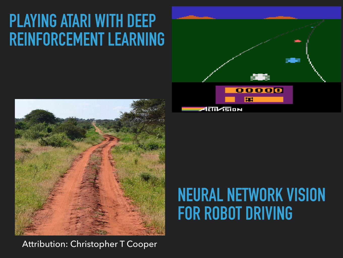
Attribution: Christopher T Cooper
NEURAL NETWORK VISION FOR ROBOT DRIVING
PLAYING ATARI WITH DEEP REINFORCEMENT LEARNING

OUTLINE
▸ Playing Atari with Deep Reinforcement Learning
▸ Motivation
▸ Intro to Reinforcement Learning (RL)
▸ Deep Q-Network (DQN)
▸ BroadMind
▸ Neural Network Vision for Robot Driving
PLAYING ATARI WITH DEEP REINFORCEMENT LEARNING
DEEPMIND

OUTLINE
▸ Playing Atari with Deep Reinforcement Learning
▸ Motivation
▸ Intro to Reinforcement Learning (RL)
▸ Deep Q-Network (DQN)
▸ BroadMind
▸ Neural Network Vision for Robot Driving
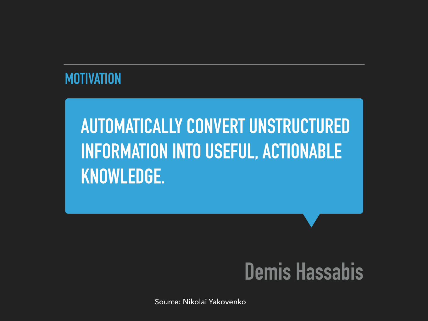
AUTOMATICALLY CONVERT UNSTRUCTURED INFORMATION INTO USEFUL, ACTIONABLE KNOWLEDGE.
Demis Hassabis
MOTIVATION
Source: Nikolai Yakovenko

CREATE AN AI SYSTEM THAT HAS THE ABILITY TO LEARN FOR ITSELF FROM EXPERIENCE.
Demis Hassabis
MOTIVATION
Source: Nikolai Yakovenko

CAN DO STUFF THAT MAYBE WE DON’T KNOW HOW TO PROGRAM.
Demis Hassabis
MOTIVATION
Source: Nikolai Yakovenko

CREATE ARTIFICIAL GENERAL INTELLIGENCE
In short,
MOTIVATION
WHY GAMES
▸ Complexity.
▸ Diversity.
▸ Easy to create more data.
▸ Meaningful reward signal.
▸ Can train and learn to transfer knowledge between similar tasks.
Adapted from Nikolai Yakovenko

OUTLINE
▸ Playing Atari with Deep Reinforcement Learning
▸ Motivation
▸ Intro to Reinforcement Learning (RL)
▸ Deep Q-Network (DQN)
▸ BroadMind
▸ Neural Network Vision for Robot Driving
AGENT AND ENVIRONMENTAgent and Environment
state
reward
action
at
rt
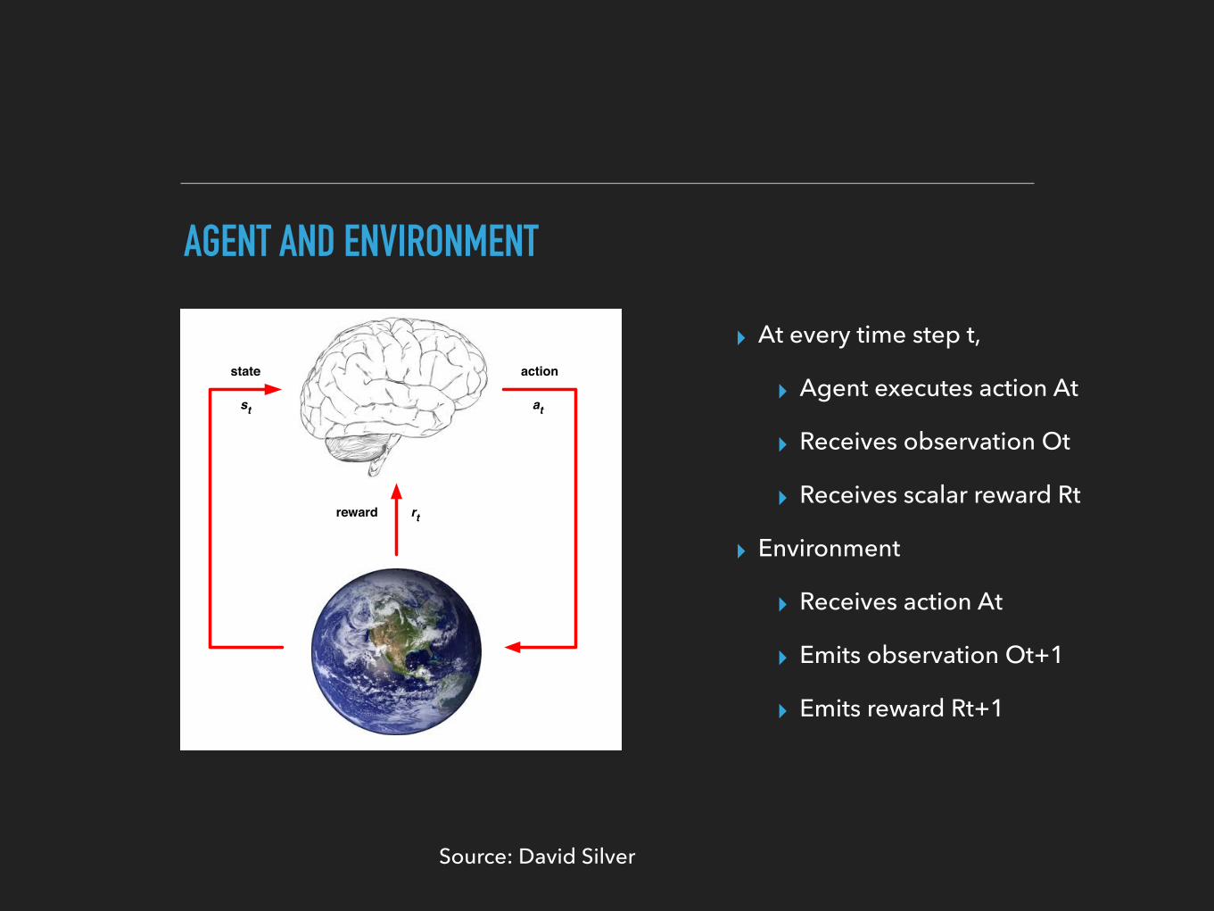
st I At each step t the agent:I Receives state stI Receives scalar reward rtI Executes action at
I The environment:I Receives action atI Emits state stI Emits scalar reward rt
▸ At every time step t,
▸ Agent executes action At
▸ Receives observation Ot
▸ Receives scalar reward Rt
▸ Environment
▸ Receives action At
▸ Emits observation Ot+1
▸ Emits reward Rt+1
Source: David Silver
REINFORCEMENT LEARNING
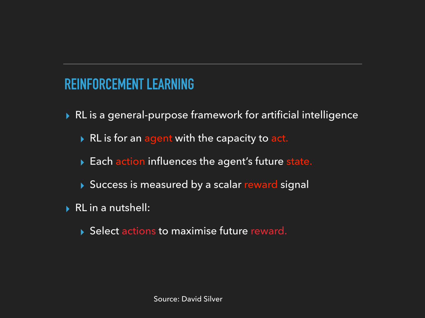
▸ RL is a general-purpose framework for artificial intelligence
▸ RL is for an agent with the capacity to act.
▸ Each action influences the agent’s future state.
▸ Success is measured by a scalar reward signal
▸ RL in a nutshell:
▸ Select actions to maximise future reward.
Source: David Silver
POLICY AND ACTION-VALUE FUNCTION
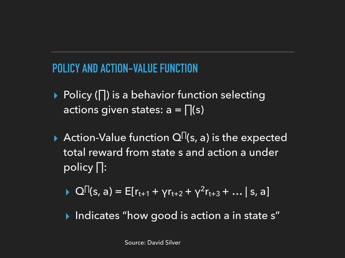
▸ Policy (∏) is a behavior function selecting actions given states: a = ∏(s)
Source: David Silver
▸ Action-Value function Q∏(s, a) is the expected total reward from state s and action a under policy ∏:
▸ Q∏(s, a) = E[rt+1 + γrt+2 + γ2rt+3 + … | s, a]
▸ Indicates “how good is action a in state s”
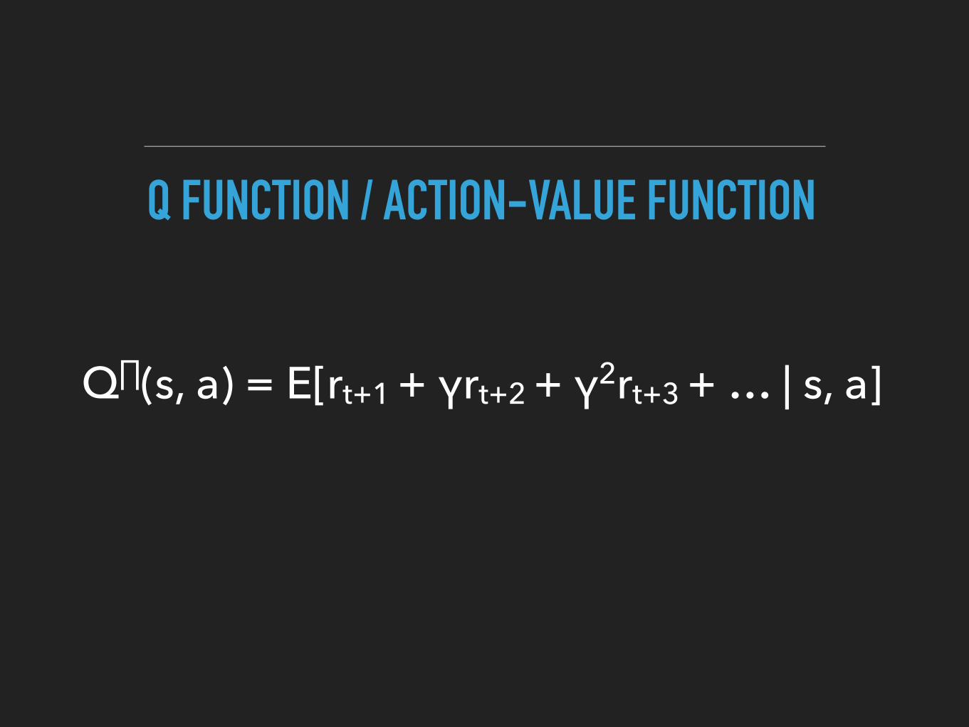
Q∏(s, a) = E[rt+1 + γrt+2 + γ2rt+3 + … | s, a]
Q FUNCTION / ACTION-VALUE FUNCTION
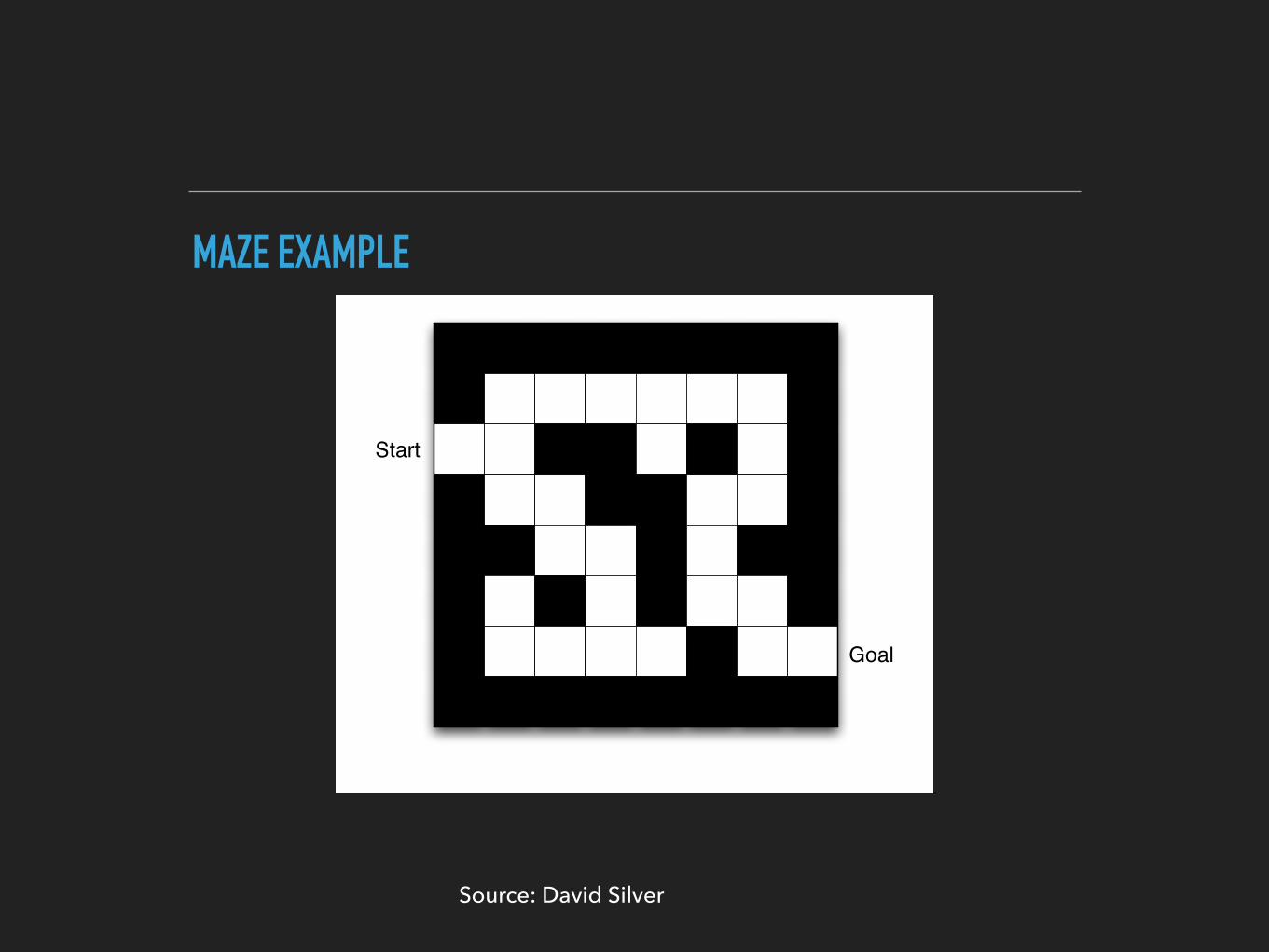
MAZE EXAMPLE
Lecture 1: Introduction to Reinforcement Learning
Inside An RL Agent
Maze Example
Start
Goal
Rewards: -1 per time-step
Actions: N, E, S, W
States: Agent’s location
Source: David Silver
TEXT
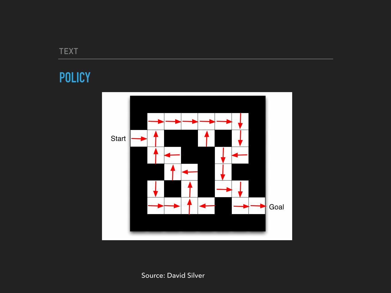
POLICY
Lecture 1: Introduction to Reinforcement Learning
Inside An RL Agent
Maze Example: Policy
Start
Goal
Arrows represent policy ⇡(s) for each state s
Source: David Silver
TEXT
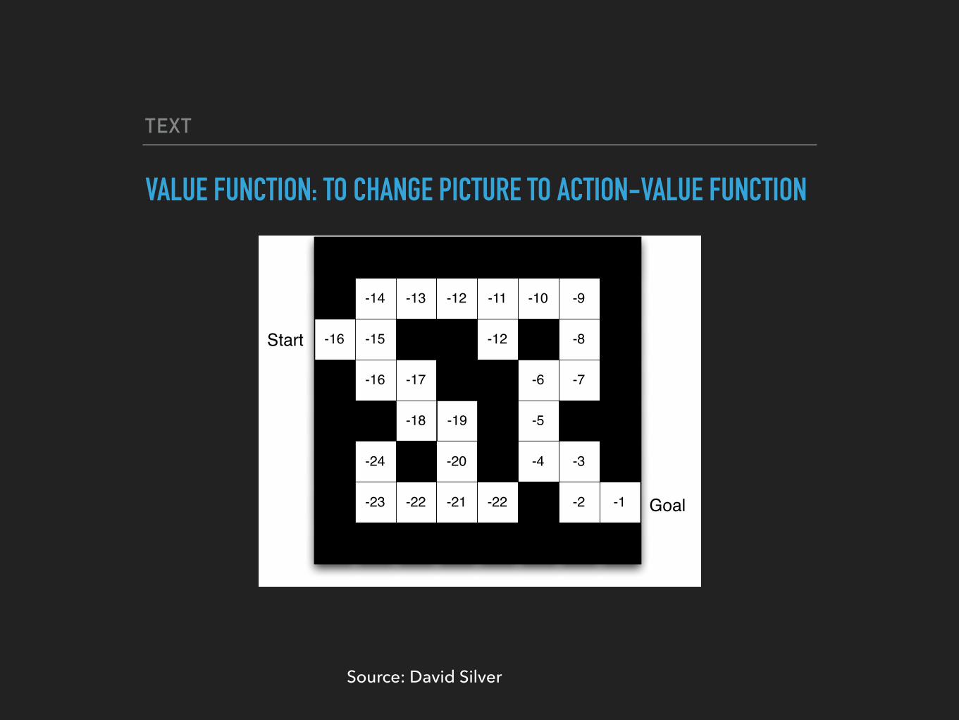
VALUE FUNCTION: TO CHANGE PICTURE TO ACTION-VALUE FUNCTION
Lecture 1: Introduction to Reinforcement Learning
Inside An RL Agent
Maze Example: Value Function
-14 -13 -12 -11 -10 -9
-16 -15 -12 -8
-16 -17 -6 -7
-18 -19 -5
-24 -20 -4 -3
-23 -22 -21 -22 -2 -1
Start
Goal
Numbers represent value v⇡(s) of each state s
Source: David Silver

TEXT
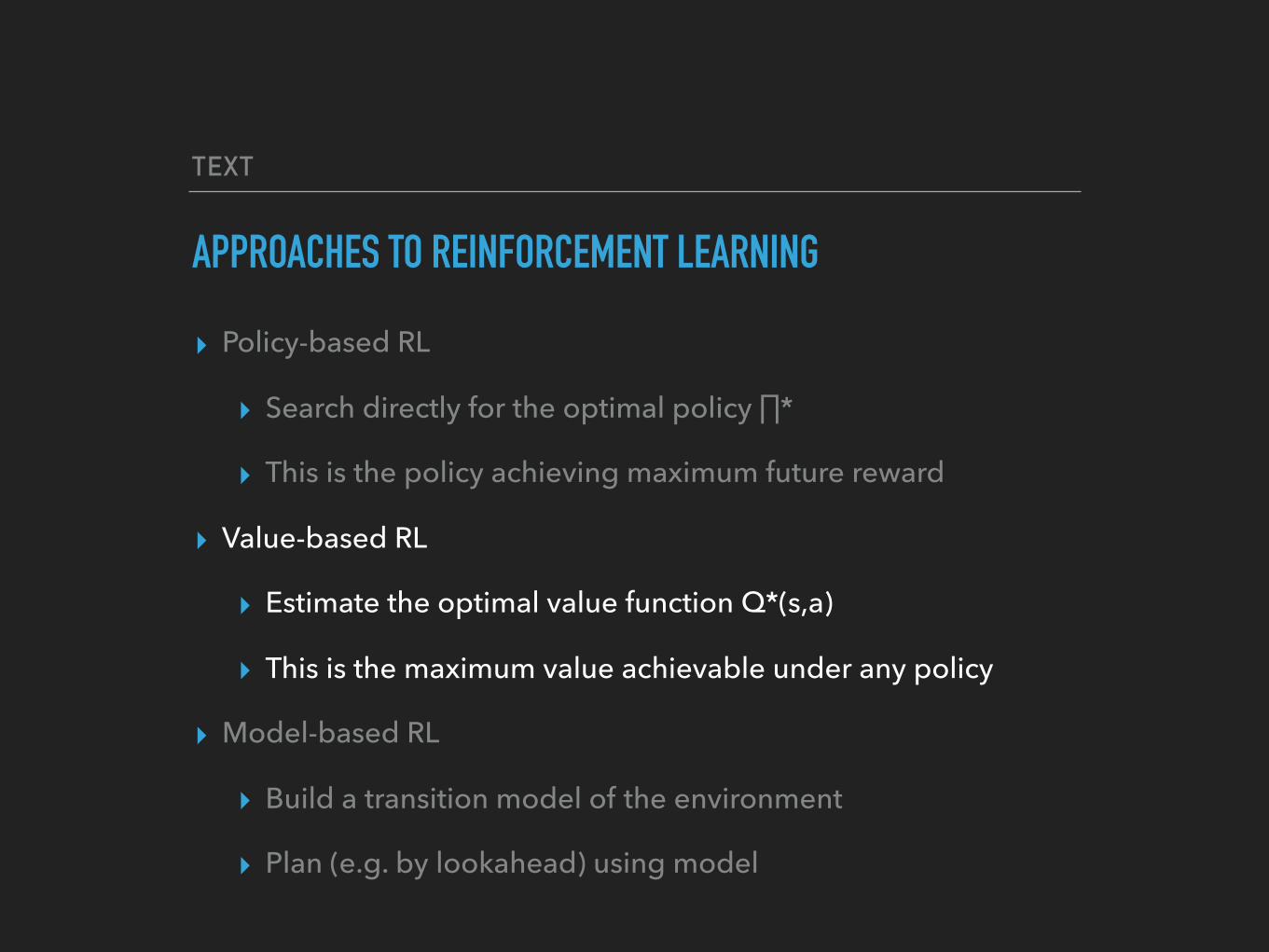
APPROACHES TO REINFORCEMENT LEARNING
▸ Policy-based RL
▸ Search directly for the optimal policy ∏*
▸ This is the policy achieving maximum future reward
▸ Value-based RL
▸ Estimate the optimal value function Q*(s,a)
▸ This is the maximum value achievable under any policy
▸ Model-based RL
▸ Build a transition model of the environment
▸ Plan (e.g. by lookahead) using model
Source: David Silver
TEXT
APPROACHES TO REINFORCEMENT LEARNING
▸ Policy-based RL
▸ Search directly for the optimal policy ∏*
▸ This is the policy achieving maximum future reward
▸ Value-based RL
▸ Estimate the optimal value function Q*(s,a)
▸ This is the maximum value achievable under any policy
▸ Model-based RL
▸ Build a transition model of the environment
▸ Plan (e.g. by lookahead) using model

OUTLINE
▸ Playing Atari with Deep Reinforcement Learning
▸ Motivation
▸ Intro to Reinforcement Learning (RL)
▸ Deep Q-Network (DQN)
▸ BroadMind
▸ Neural Network Vision for Robot Driving
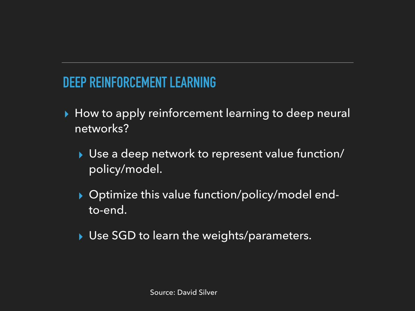
DEEP REINFORCEMENT LEARNING
▸ How to apply reinforcement learning to deep neural networks?
▸ Use a deep network to represent value function/policy/model.
▸ Optimize this value function/policy/model end-to-end.
▸ Use SGD to learn the weights/parameters.
Source: David Silver
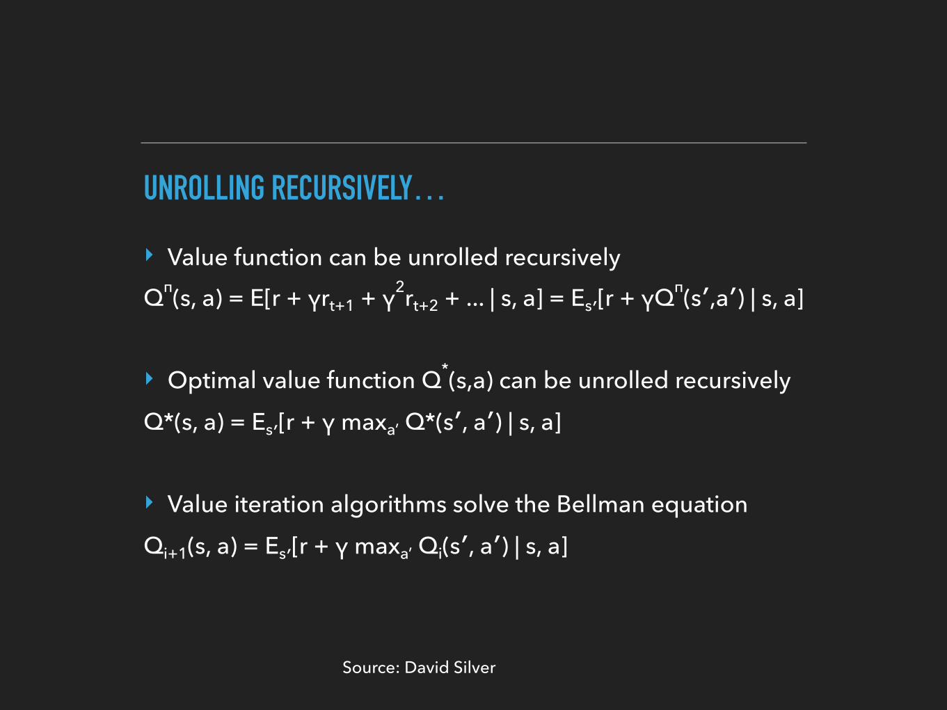
UNROLLING RECURSIVELY…
‣ Value function can be unrolled recursively Qπ(s, a) = E[r + γrt+1 + γ2rt+2 + ... | s, a] = Es′[r + γQπ(s′,a′) | s, a]
‣ Optimal value function Q*(s,a) can be unrolled recursively Q*(s, a) = Es′[r + γ maxa’ Q*(s′, a′) | s, a]
‣ Value iteration algorithms solve the Bellman equation Qi+1(s, a) = Es′[r + γ maxa’ Qi(s′, a′) | s, a]
Source: David Silver
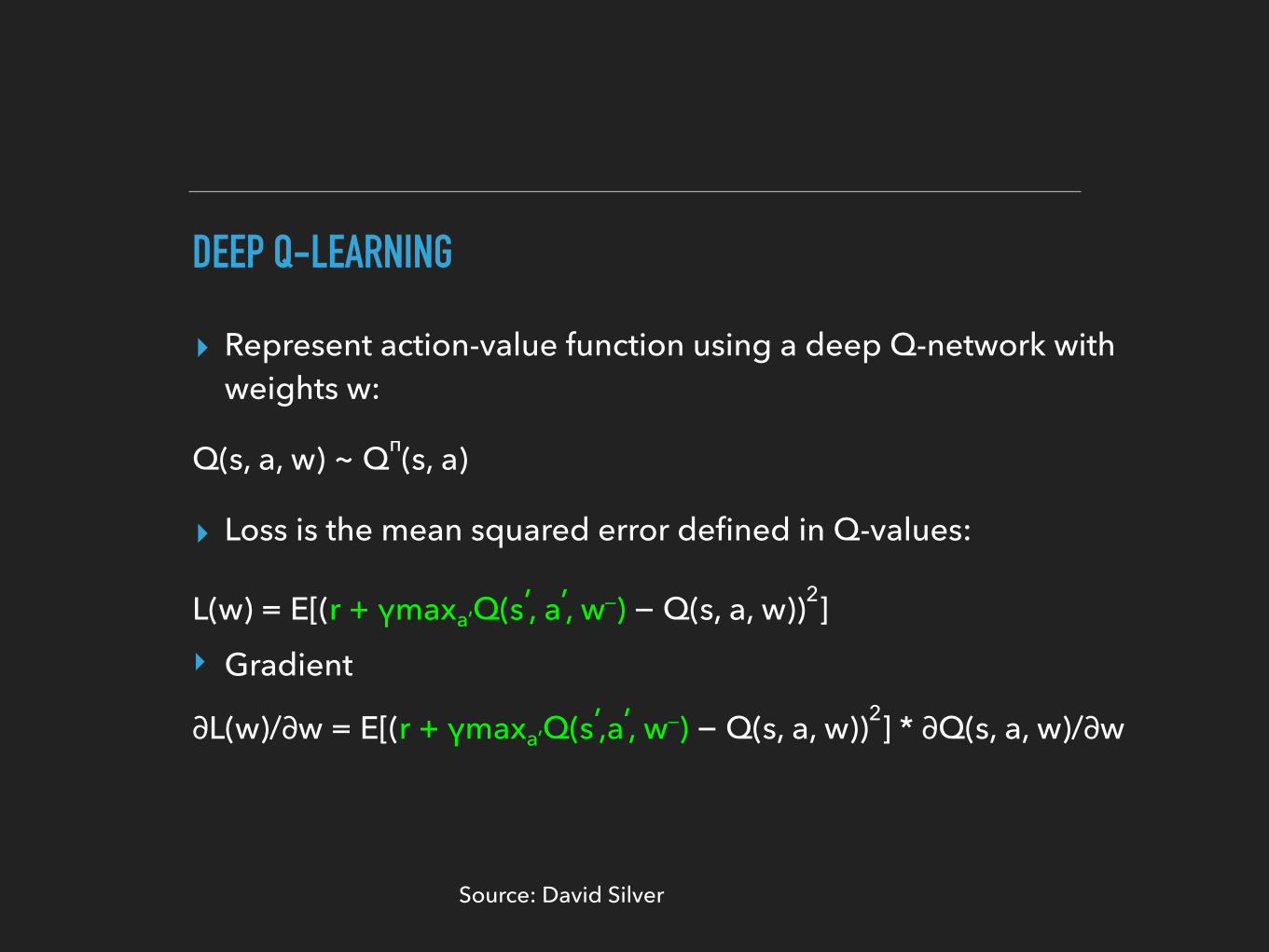
DEEP Q-LEARNING
▸ Represent action-value function using a deep Q-network with weights w:
Q(s, a, w) ~ Qπ(s, a)
▸ Loss is the mean squared error defined in Q-values:
L(w) = E[(r + γmaxa’Q(s’, a’, w_) − Q(s, a, w))2] ‣ Gradient
∂L(w)/∂w = E[(r + γmaxa’Q(s’,a’, w_) − Q(s, a, w))2] * ∂Q(s, a, w)/∂w
Source: David Silver
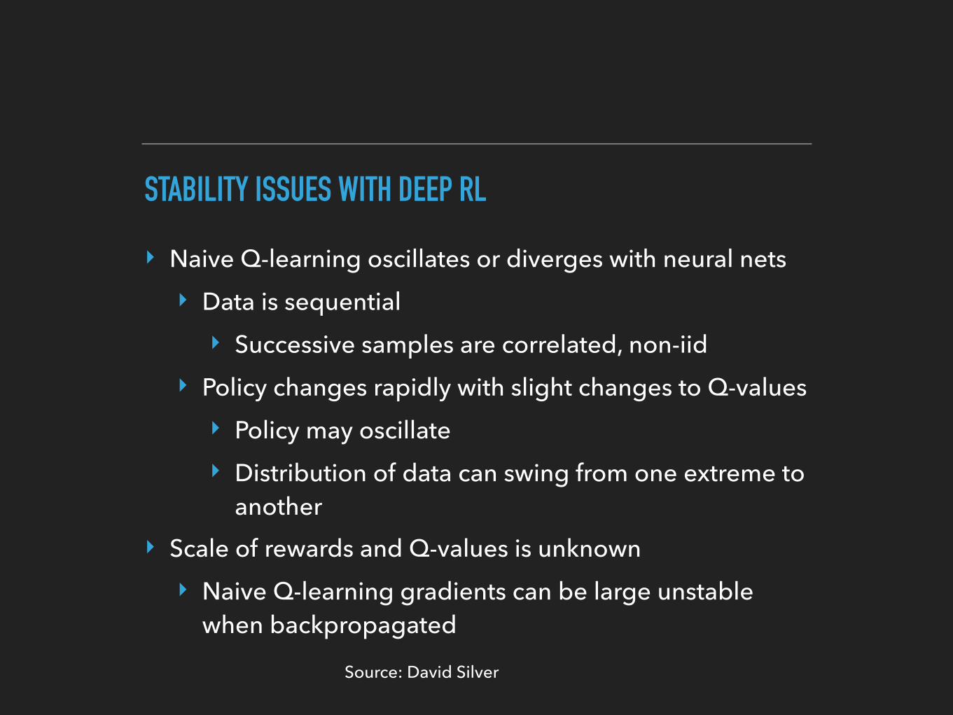
STABILITY ISSUES WITH DEEP RL
‣ Naive Q-learning oscillates or diverges with neural nets ‣ Data is sequential ‣ Successive samples are correlated, non-iid
‣ Policy changes rapidly with slight changes to Q-values ‣ Policy may oscillate ‣ Distribution of data can swing from one extreme to
another ‣ Scale of rewards and Q-values is unknown ‣ Naive Q-learning gradients can be large unstable
when backpropagated
Source: David Silver
TEXT
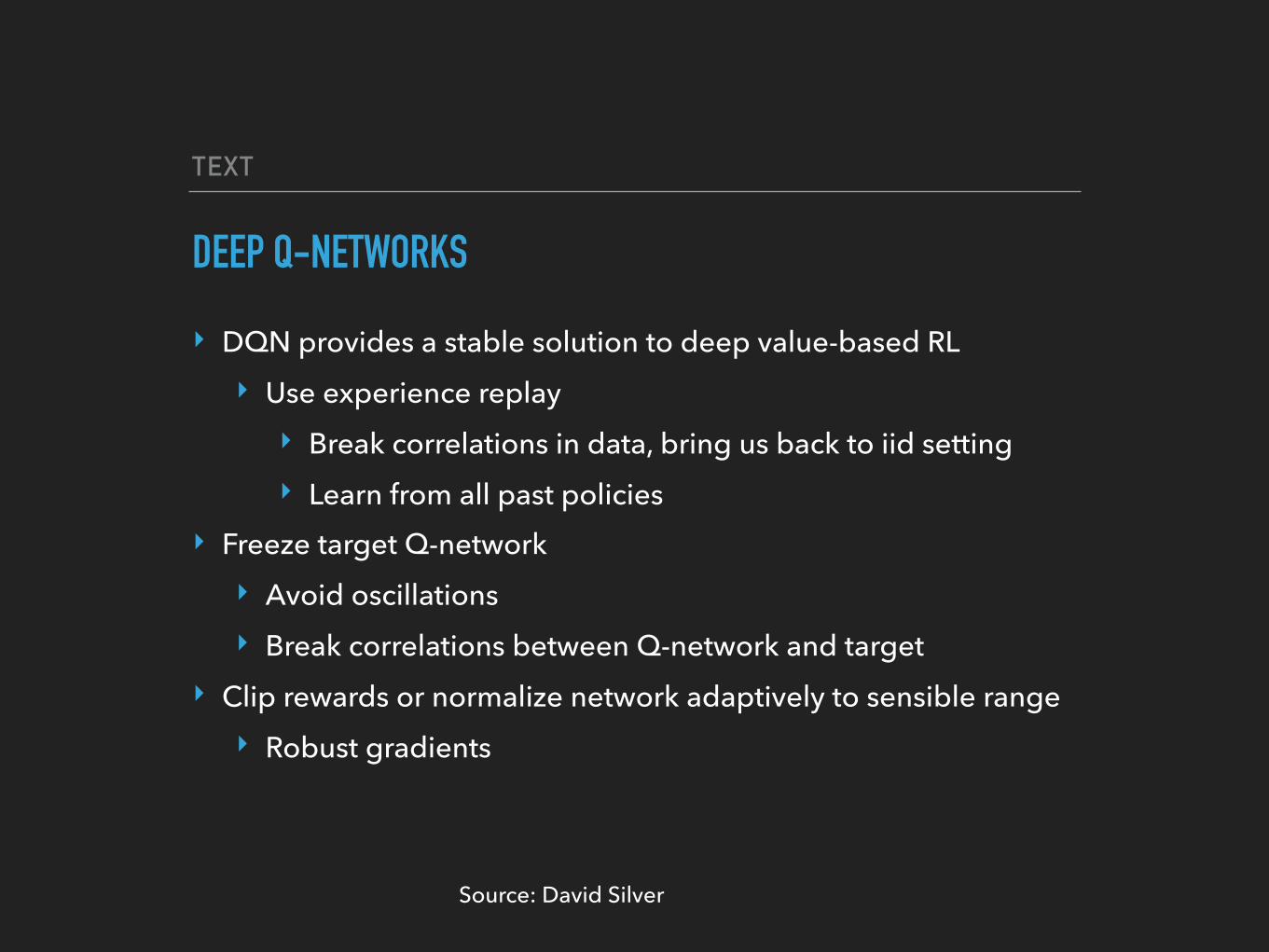
DEEP Q-NETWORKS
‣ DQN provides a stable solution to deep value-based RL ‣ Use experience replay ‣ Break correlations in data, bring us back to iid setting ‣ Learn from all past policies
‣ Freeze target Q-network ‣ Avoid oscillations ‣ Break correlations between Q-network and target
‣ Clip rewards or normalize network adaptively to sensible range ‣ Robust gradients
Source: David Silver
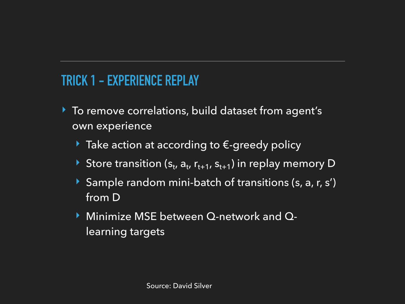
TRICK 1 - EXPERIENCE REPLAY
‣ To remove correlations, build dataset from agent’s own experience ‣ Take action at according to €-greedy policy ‣ Store transition (st, at, rt+1, st+1) in replay memory D ‣ Sample random mini-batch of transitions (s, a, r, s’)
from D ‣ Minimize MSE between Q-network and Q-
learning targets
Source: David Silver
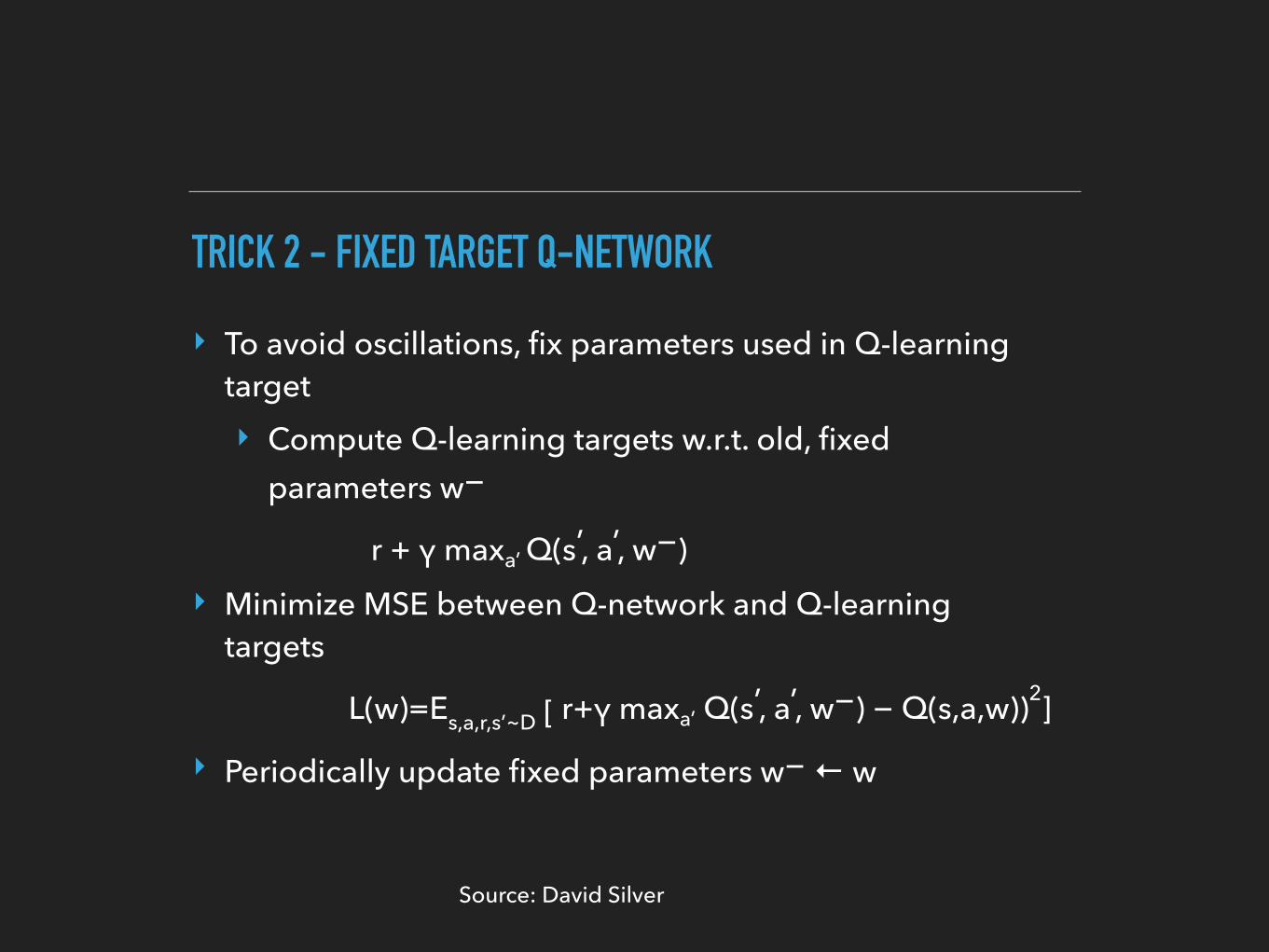
TRICK 2 - FIXED TARGET Q-NETWORK
‣ To avoid oscillations, fix parameters used in Q-learning target ‣ Compute Q-learning targets w.r.t. old, fixed
parameters w−
r + γ maxa’ Q(s’, a’, w−) ‣ Minimize MSE between Q-network and Q-learning
targets
L(w)=Es,a,r,s’~D [ r+γ maxa’ Q(s’, a’, w−) − Q(s,a,w))2]
‣ Periodically update fixed parameters w− ← w
Source: David Silver

TRICK 3 - REWARD/VALUE RANGE
‣ Advantages ‣ DQN clips the rewards to [−1,+1] ‣ This prevents Q-values from becoming too large ‣ Ensures gradients are well-conditioned
‣ Disadvantages ‣ Can’t tell difference between small and large
rewards
Source: David Silver

BACK TO BROADMINDReinforcement Learning in Atari
state
reward
action
at
rt
st
Source: David Silver
INTRODUCTION - ATARI AGENT (AKA BROADMIND)
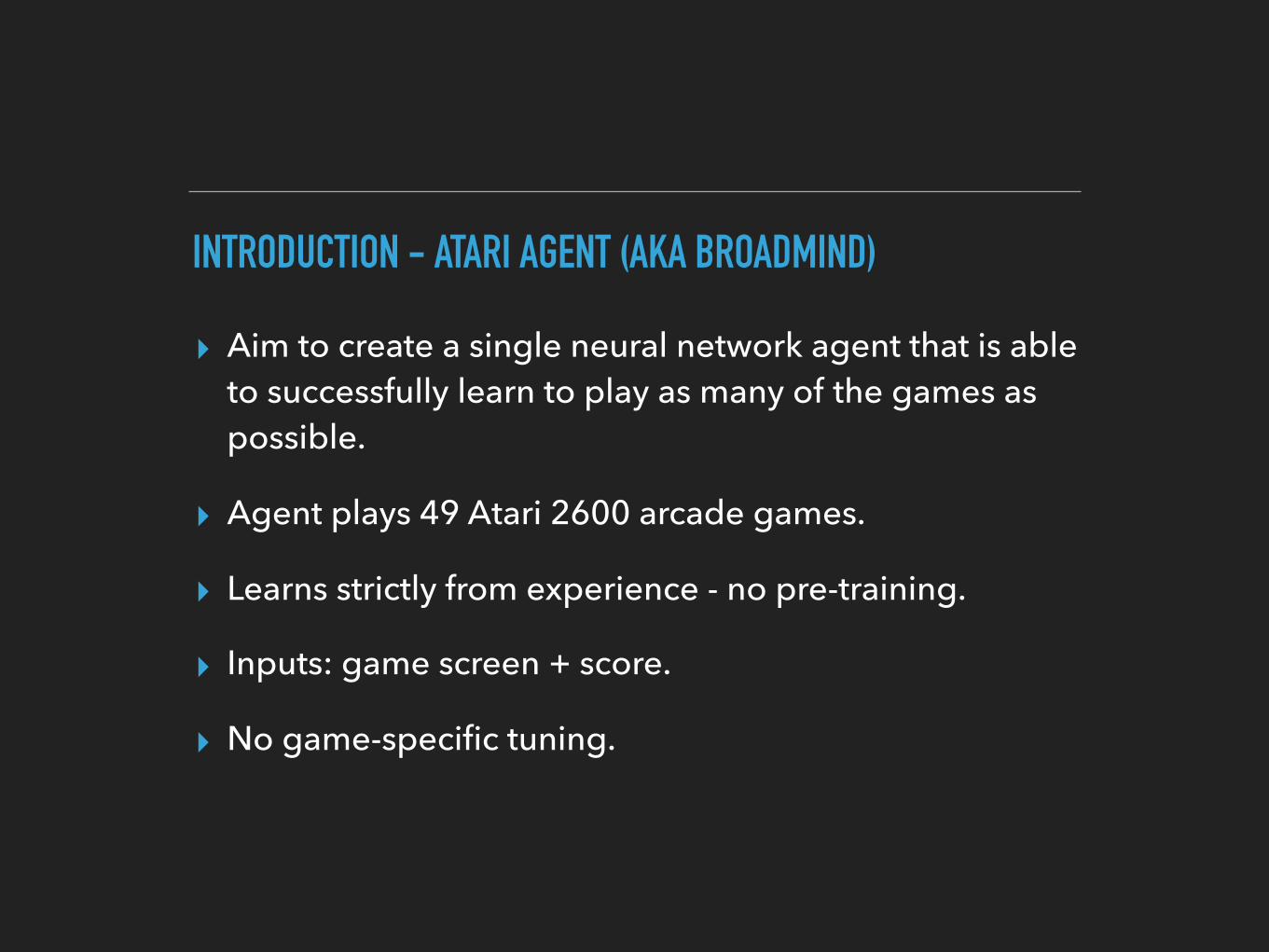
▸ Aim to create a single neural network agent that is able to successfully learn to play as many of the games as possible.
▸ Agent plays 49 Atari 2600 arcade games.
▸ Learns strictly from experience - no pre-training.
▸ Inputs: game screen + score.
▸ No game-specific tuning.
INTRODUCTION - ATARI AGENT (AKA BROADMIND)
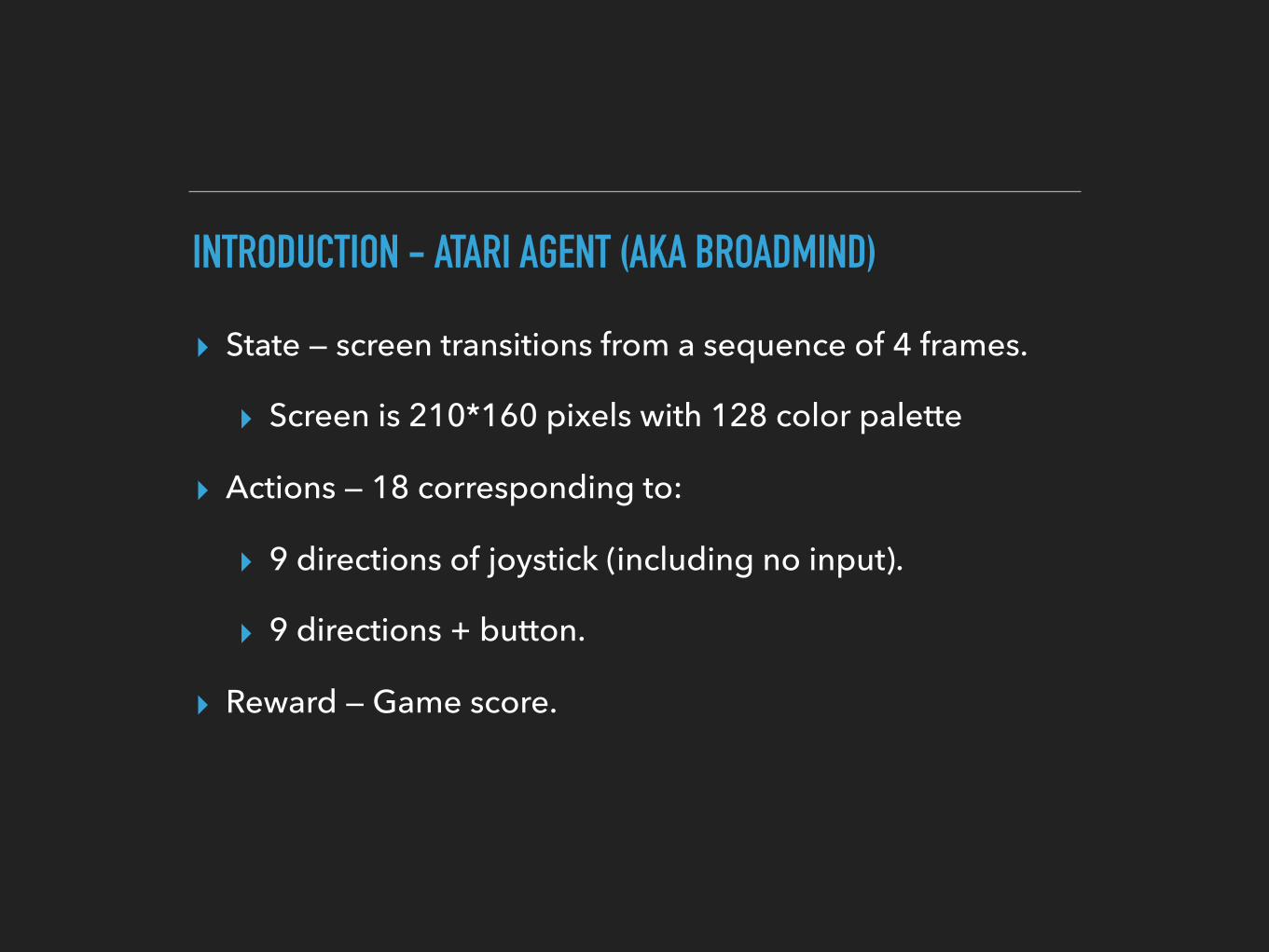
▸ State — screen transitions from a sequence of 4 frames.
▸ Screen is 210*160 pixels with 128 color palette
▸ Actions — 18 corresponding to:
▸ 9 directions of joystick (including no input).
▸ 9 directions + button.
▸ Reward — Game score.
difficult and engaging for human players. We used the same networkarchitecture, hyperparameter values (see Extended Data Table 1) andlearning procedure throughout—taking high-dimensional data (210|160colour video at 60 Hz) as input—to demonstrate that our approachrobustly learns successful policies over a variety of games based solelyon sensory inputs with only very minimal prior knowledge (that is, merelythe input data were visual images, and the number of actions availablein each game, but not their correspondences; see Methods). Notably,our method was able to train large neural networks using a reinforce-ment learning signal and stochastic gradient descent in a stable manner—illustrated by the temporal evolution of two indices of learning (theagent’s average score-per-episode and average predicted Q-values; seeFig. 2 and Supplementary Discussion for details).
We compared DQN with the best performing methods from thereinforcement learning literature on the 49 games where results wereavailable12,15. In addition to the learned agents, we also report scores fora professional human games tester playing under controlled conditionsand a policy that selects actions uniformly at random (Extended DataTable 2 and Fig. 3, denoted by 100% (human) and 0% (random) on yaxis; see Methods). Our DQN method outperforms the best existingreinforcement learning methods on 43 of the games without incorpo-rating any of the additional prior knowledge about Atari 2600 gamesused by other approaches (for example, refs 12, 15). Furthermore, ourDQN agent performed at a level that was comparable to that of a pro-fessional human games tester across the set of 49 games, achieving morethan 75% of the human score on more than half of the games (29 games;
Convolution Convolution Fully connected Fully connected
No input
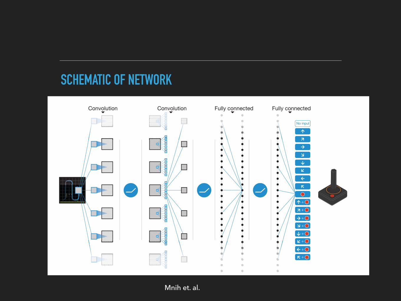
Figure 1 | Schematic illustration of the convolutional neural network. Thedetails of the architecture are explained in the Methods. The input to the neuralnetwork consists of an 84 3 84 3 4 image produced by the preprocessingmap w, followed by three convolutional layers (note: snaking blue line
symbolizes sliding of each filter across input image) and two fully connectedlayers with a single output for each valid action. Each hidden layer is followedby a rectifier nonlinearity (that is, max 0,xð Þ).
a b
c d
0 200 400 600 800
1,000 1,200 1,400 1,600 1,800 2,000 2,200
0 20 40 60 80 100 120 140 160 180 200
Ave
rage
sco
re p
er e
piso
de
Training epochs
0 1 2 3 4 5 6 7 8 9
10 11
0 20 40 60 80 100 120 140 160 180 200
Ave
rage
act
ion
valu
e (Q
)
Training epochs
0
1,000
2,000
3,000
4,000
5,000
6,000
0 20 40 60 80 100 120 140 160 180 200
Ave
rage
sco
re p
er e
piso
de
Training epochs
0 1 2 3 4 5 6 7 8 9
10
0 20 40 60 80 100 120 140 160 180 200
Ave
rage
act
ion
valu
e (Q
)
Training epochs
Figure 2 | Training curves tracking the agent’s average score and averagepredicted action-value. a, Each point is the average score achieved per episodeafter the agent is run with e-greedy policy (e 5 0.05) for 520 k frames on SpaceInvaders. b, Average score achieved per episode for Seaquest. c, Averagepredicted action-value on a held-out set of states on Space Invaders. Each point
on the curve is the average of the action-value Q computed over the held-outset of states. Note that Q-values are scaled due to clipping of rewards (seeMethods). d, Average predicted action-value on Seaquest. See SupplementaryDiscussion for details.
RESEARCH LETTER
5 3 0 | N A T U R E | V O L 5 1 8 | 2 6 F E B R U A R Y 2 0 1 5
Macmillan Publishers Limited. All rights reserved©2015
SCHEMATIC OF NETWORK
Mnih et. al.

NETWORK ARCHITECTURE
DQN in Atari
I End-to-end learning of values Q(s, a) from pixels s
I Input state s is stack of raw pixels from last 4 frames
I Output is Q(s, a) for 18 joystick/button positions
I Reward is change in score for that step
Network architecture and hyperparameters fixed across all games[Mnih et al.]
Mnih et. al.
EVALUATION
0
50
100
150
200
250
0 10 20 30 40 50 60 70 80 90 100
Ave
rage R
ew
ard
per
Epis
ode
Training Epochs
Average Reward on Breakout
0
200
400
600
800
1000
1200
1400
1600
1800
0 10 20 30 40 50 60 70 80 90 100A
vera
ge R
ew
ard
per
Epis
ode
Training Epochs
Average Reward on Seaquest
0
0.5
1
1.5
2
2.5
3
3.5
4
0 10 20 30 40 50 60 70 80 90 100
Ave
rage A
ctio
n V
alu
e (
Q)
Training Epochs
Average Q on Breakout
0
1
2
3
4
5
6
7
8
9
0 10 20 30 40 50 60 70 80 90 100
Ave
rage A
ctio
n V
alu
e (
Q)
Training Epochs
Average Q on Seaquest
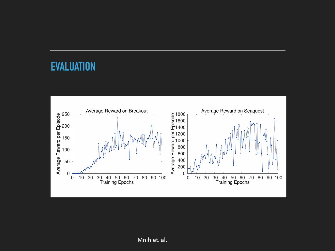
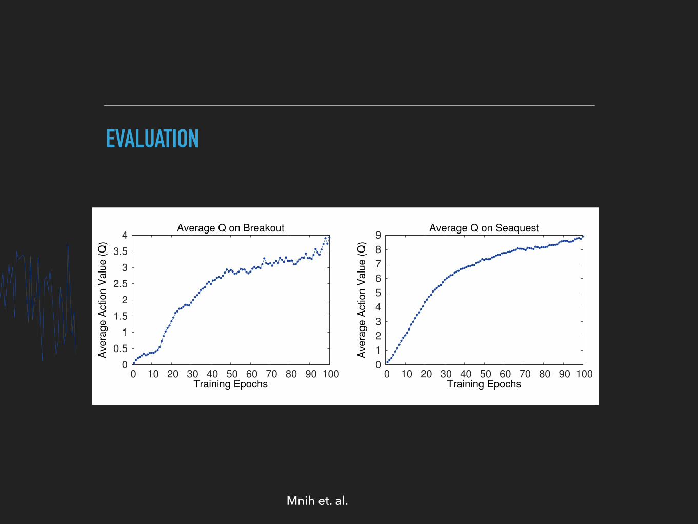
Figure 2: The two plots on the left show average reward per episode on Breakout and Seaquestrespectively during training. The statistics were computed by running an ✏-greedy policy with ✏ =
0.05 for 10000 steps. The two plots on the right show the average maximum predicted action-valueof a held out set of states on Breakout and Seaquest respectively. One epoch corresponds to 50000minibatch weight updates or roughly 30 minutes of training time.
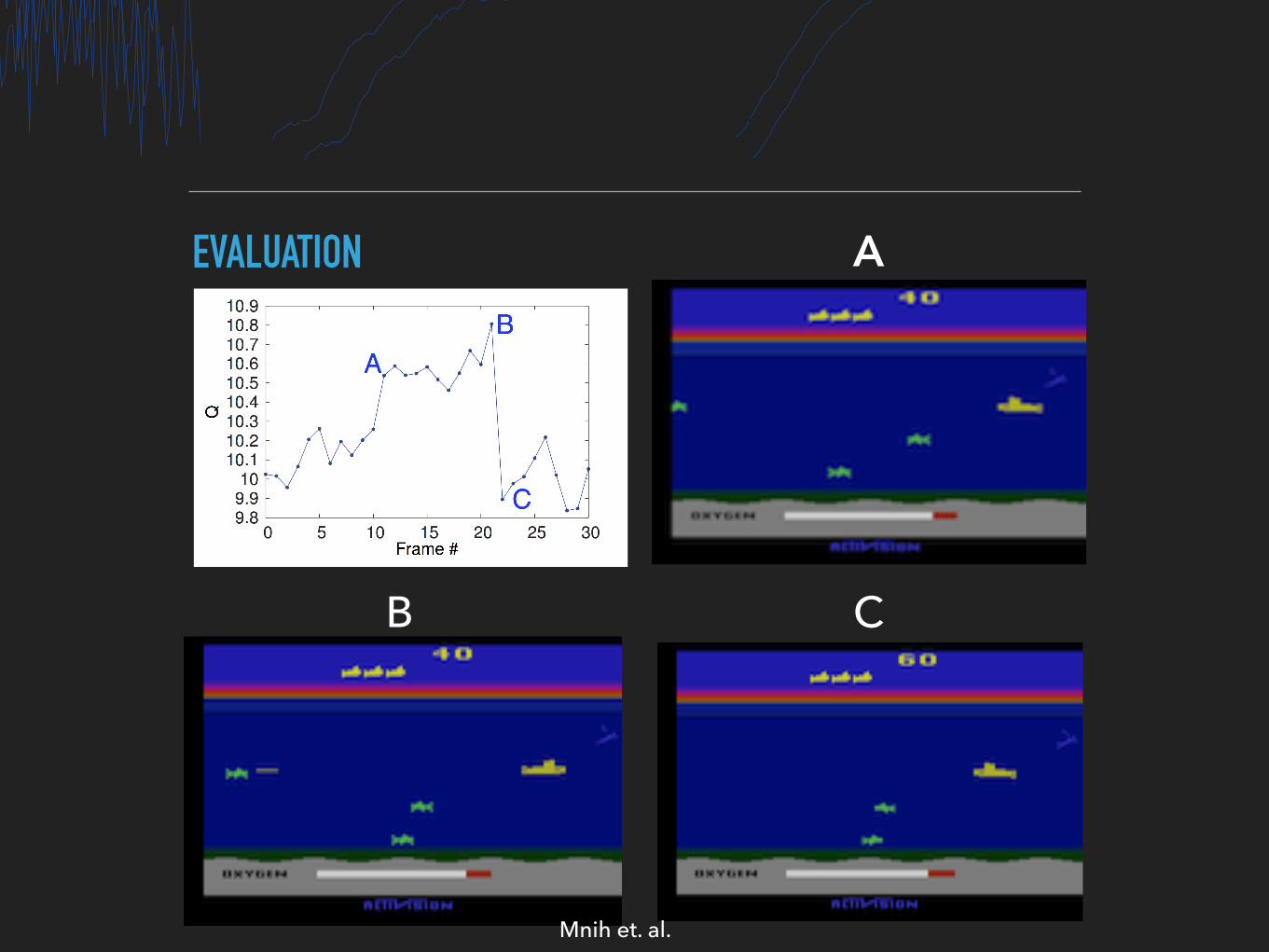
Figure 3: The leftmost plot shows the predicted value function for a 30 frame segment of the gameSeaquest. The three screenshots correspond to the frames labeled by A, B, and C respectively.
5.2 Visualizing the Value Function
Figure 3 shows a visualization of the learned value function on the game Seaquest. The figure showsthat the predicted value jumps after an enemy appears on the left of the screen (point A). The agentthen fires a torpedo at the enemy and the predicted value peaks as the torpedo is about to hit theenemy (point B). Finally, the value falls to roughly its original value after the enemy disappears(point C). Figure 3 demonstrates that our method is able to learn how the value function evolves fora reasonably complex sequence of events.
5.3 Main Evaluation
We compare our results with the best performing methods from the RL literature [3, 4]. The methodlabeled Sarsa used the Sarsa algorithm to learn linear policies on several different feature sets hand-engineered for the Atari task and we report the score for the best performing feature set [3]. Con-tingency used the same basic approach as Sarsa but augmented the feature sets with a learnedrepresentation of the parts of the screen that are under the agent’s control [4]. Note that both of thesemethods incorporate significant prior knowledge about the visual problem by using background sub-traction and treating each of the 128 colors as a separate channel. Since many of the Atari games useone distinct color for each type of object, treating each color as a separate channel can be similar toproducing a separate binary map encoding the presence of each object type. In contrast, our agentsonly receive the raw RGB screenshots as input and must learn to detect objects on their own.
In addition to the learned agents, we also report scores for an expert human game player and a policythat selects actions uniformly at random. The human performance is the median reward achievedafter around two hours of playing each game. Note that our reported human scores are much higherthan the ones in Bellemare et al. [3]. For the learned methods, we follow the evaluation strategy usedin Bellemare et al. [3, 5] and report the average score obtained by running an ✏-greedy policy with✏ = 0.05 for a fixed number of steps. The first five rows of table 1 show the per-game average scoreson all games. Our approach (labeled DQN) outperforms the other learning methods by a substantialmargin on all seven games despite incorporating almost no prior knowledge about the inputs.
We also include a comparison to the evolutionary policy search approach from [8] in the last threerows of table 1. We report two sets of results for this method. The HNeat Best score reflects theresults obtained by using a hand-engineered object detector algorithm that outputs the locations and
7
Mnih et. al.
EVALUATION
0
50
100
150
200
250
0 10 20 30 40 50 60 70 80 90 100
Ave
rag
e R
ew
ard
pe
r E
pis
od
e
Training Epochs
Average Reward on Breakout
0
200
400
600
800
1000
1200
1400
1600
1800
0 10 20 30 40 50 60 70 80 90 100
Ave
rag
e R
ew
ard
pe
r E
pis
od
e
Training Epochs
Average Reward on Seaquest
0
0.5
1
1.5
2
2.5
3
3.5
4
0 10 20 30 40 50 60 70 80 90 100
Ave
rag
e A
ctio
n V
alu
e (
Q)
Training Epochs
Average Q on Breakout
0
1
2
3
4
5
6
7
8
9
0 10 20 30 40 50 60 70 80 90 100A
vera
ge
Act
ion
Va
lue
(Q
)
Training Epochs
Average Q on Seaquest
Figure 2: The two plots on the left show average reward per episode on Breakout and Seaquestrespectively during training. The statistics were computed by running an ✏-greedy policy with ✏ =
0.05 for 10000 steps. The two plots on the right show the average maximum predicted action-valueof a held out set of states on Breakout and Seaquest respectively. One epoch corresponds to 50000minibatch weight updates or roughly 30 minutes of training time.
Figure 3: The leftmost plot shows the predicted value function for a 30 frame segment of the gameSeaquest. The three screenshots correspond to the frames labeled by A, B, and C respectively.
5.2 Visualizing the Value Function
Figure 3 shows a visualization of the learned value function on the game Seaquest. The figure showsthat the predicted value jumps after an enemy appears on the left of the screen (point A). The agentthen fires a torpedo at the enemy and the predicted value peaks as the torpedo is about to hit theenemy (point B). Finally, the value falls to roughly its original value after the enemy disappears(point C). Figure 3 demonstrates that our method is able to learn how the value function evolves fora reasonably complex sequence of events.
5.3 Main Evaluation
We compare our results with the best performing methods from the RL literature [3, 4]. The methodlabeled Sarsa used the Sarsa algorithm to learn linear policies on several different feature sets hand-engineered for the Atari task and we report the score for the best performing feature set [3]. Con-tingency used the same basic approach as Sarsa but augmented the feature sets with a learnedrepresentation of the parts of the screen that are under the agent’s control [4]. Note that both of thesemethods incorporate significant prior knowledge about the visual problem by using background sub-traction and treating each of the 128 colors as a separate channel. Since many of the Atari games useone distinct color for each type of object, treating each color as a separate channel can be similar toproducing a separate binary map encoding the presence of each object type. In contrast, our agentsonly receive the raw RGB screenshots as input and must learn to detect objects on their own.
In addition to the learned agents, we also report scores for an expert human game player and a policythat selects actions uniformly at random. The human performance is the median reward achievedafter around two hours of playing each game. Note that our reported human scores are much higherthan the ones in Bellemare et al. [3]. For the learned methods, we follow the evaluation strategy usedin Bellemare et al. [3, 5] and report the average score obtained by running an ✏-greedy policy with✏ = 0.05 for a fixed number of steps. The first five rows of table 1 show the per-game average scoreson all games. Our approach (labeled DQN) outperforms the other learning methods by a substantialmargin on all seven games despite incorporating almost no prior knowledge about the inputs.
We also include a comparison to the evolutionary policy search approach from [8] in the last threerows of table 1. We report two sets of results for this method. The HNeat Best score reflects theresults obtained by using a hand-engineered object detector algorithm that outputs the locations and
7
Mnih et. al.
EVALUATION
0
50
100
150
200
250
0 10 20 30 40 50 60 70 80 90 100
Ave
rage R
ew
ard
per
Epis
ode
Training Epochs
Average Reward on Breakout
0
200
400
600
800
1000
1200
1400
1600
1800
0 10 20 30 40 50 60 70 80 90 100
Ave
rage R
ew
ard
per
Epis
ode
Training Epochs
Average Reward on Seaquest
0
0.5
1
1.5
2
2.5
3
3.5
4
0 10 20 30 40 50 60 70 80 90 100
Ave
rage A
ctio
n V
alu
e (
Q)
Training Epochs
Average Q on Breakout
0
1
2
3
4
5
6
7
8
9
0 10 20 30 40 50 60 70 80 90 100
Ave
rage A
ctio
n V
alu
e (
Q)
Training Epochs
Average Q on Seaquest
Figure 2: The two plots on the left show average reward per episode on Breakout and Seaquestrespectively during training. The statistics were computed by running an ✏-greedy policy with ✏ =
0.05 for 10000 steps. The two plots on the right show the average maximum predicted action-valueof a held out set of states on Breakout and Seaquest respectively. One epoch corresponds to 50000minibatch weight updates or roughly 30 minutes of training time.
Figure 3: The leftmost plot shows the predicted value function for a 30 frame segment of the gameSeaquest. The three screenshots correspond to the frames labeled by A, B, and C respectively.
5.2 Visualizing the Value Function
Figure 3 shows a visualization of the learned value function on the game Seaquest. The figure showsthat the predicted value jumps after an enemy appears on the left of the screen (point A). The agentthen fires a torpedo at the enemy and the predicted value peaks as the torpedo is about to hit theenemy (point B). Finally, the value falls to roughly its original value after the enemy disappears(point C). Figure 3 demonstrates that our method is able to learn how the value function evolves fora reasonably complex sequence of events.
5.3 Main Evaluation
We compare our results with the best performing methods from the RL literature [3, 4]. The methodlabeled Sarsa used the Sarsa algorithm to learn linear policies on several different feature sets hand-engineered for the Atari task and we report the score for the best performing feature set [3]. Con-tingency used the same basic approach as Sarsa but augmented the feature sets with a learnedrepresentation of the parts of the screen that are under the agent’s control [4]. Note that both of thesemethods incorporate significant prior knowledge about the visual problem by using background sub-traction and treating each of the 128 colors as a separate channel. Since many of the Atari games useone distinct color for each type of object, treating each color as a separate channel can be similar toproducing a separate binary map encoding the presence of each object type. In contrast, our agentsonly receive the raw RGB screenshots as input and must learn to detect objects on their own.
In addition to the learned agents, we also report scores for an expert human game player and a policythat selects actions uniformly at random. The human performance is the median reward achievedafter around two hours of playing each game. Note that our reported human scores are much higherthan the ones in Bellemare et al. [3]. For the learned methods, we follow the evaluation strategy usedin Bellemare et al. [3, 5] and report the average score obtained by running an ✏-greedy policy with✏ = 0.05 for a fixed number of steps. The first five rows of table 1 show the per-game average scoreson all games. Our approach (labeled DQN) outperforms the other learning methods by a substantialmargin on all seven games despite incorporating almost no prior knowledge about the inputs.
We also include a comparison to the evolutionary policy search approach from [8] in the last threerows of table 1. We report two sets of results for this method. The HNeat Best score reflects theresults obtained by using a hand-engineered object detector algorithm that outputs the locations and
7
0
50
100
150
200
250
0 10 20 30 40 50 60 70 80 90 100
Ave
rag
e R
ew
ard
pe
r E
pis
od
e
Training Epochs
Average Reward on Breakout
0
200
400
600
800
1000
1200
1400
1600
1800
0 10 20 30 40 50 60 70 80 90 100
Ave
rag
e R
ew
ard
pe
r E
pis
od
e
Training Epochs
Average Reward on Seaquest
0
0.5
1
1.5
2
2.5
3
3.5
4
0 10 20 30 40 50 60 70 80 90 100
Ave
rag
e A
ctio
n V
alu
e (
Q)
Training Epochs
Average Q on Breakout
0
1
2
3
4
5
6
7
8
9
0 10 20 30 40 50 60 70 80 90 100
Ave
rag
e A
ctio
n V
alu
e (
Q)
Training Epochs
Average Q on Seaquest
Figure 2: The two plots on the left show average reward per episode on Breakout and Seaquestrespectively during training. The statistics were computed by running an ✏-greedy policy with ✏ =
0.05 for 10000 steps. The two plots on the right show the average maximum predicted action-valueof a held out set of states on Breakout and Seaquest respectively. One epoch corresponds to 50000minibatch weight updates or roughly 30 minutes of training time.
Figure 3: The leftmost plot shows the predicted value function for a 30 frame segment of the gameSeaquest. The three screenshots correspond to the frames labeled by A, B, and C respectively.
5.2 Visualizing the Value Function
Figure 3 shows a visualization of the learned value function on the game Seaquest. The figure showsthat the predicted value jumps after an enemy appears on the left of the screen (point A). The agentthen fires a torpedo at the enemy and the predicted value peaks as the torpedo is about to hit theenemy (point B). Finally, the value falls to roughly its original value after the enemy disappears(point C). Figure 3 demonstrates that our method is able to learn how the value function evolves fora reasonably complex sequence of events.
5.3 Main Evaluation
We compare our results with the best performing methods from the RL literature [3, 4]. The methodlabeled Sarsa used the Sarsa algorithm to learn linear policies on several different feature sets hand-engineered for the Atari task and we report the score for the best performing feature set [3]. Con-tingency used the same basic approach as Sarsa but augmented the feature sets with a learnedrepresentation of the parts of the screen that are under the agent’s control [4]. Note that both of thesemethods incorporate significant prior knowledge about the visual problem by using background sub-traction and treating each of the 128 colors as a separate channel. Since many of the Atari games useone distinct color for each type of object, treating each color as a separate channel can be similar toproducing a separate binary map encoding the presence of each object type. In contrast, our agentsonly receive the raw RGB screenshots as input and must learn to detect objects on their own.
In addition to the learned agents, we also report scores for an expert human game player and a policythat selects actions uniformly at random. The human performance is the median reward achievedafter around two hours of playing each game. Note that our reported human scores are much higherthan the ones in Bellemare et al. [3]. For the learned methods, we follow the evaluation strategy usedin Bellemare et al. [3, 5] and report the average score obtained by running an ✏-greedy policy with✏ = 0.05 for a fixed number of steps. The first five rows of table 1 show the per-game average scoreson all games. Our approach (labeled DQN) outperforms the other learning methods by a substantialmargin on all seven games despite incorporating almost no prior knowledge about the inputs.
We also include a comparison to the evolutionary policy search approach from [8] in the last threerows of table 1. We report two sets of results for this method. The HNeat Best score reflects theresults obtained by using a hand-engineered object detector algorithm that outputs the locations and
7
0
50
100
150
200
250
0 10 20 30 40 50 60 70 80 90 100
Ave
rage R
ew
ard
per
Epis
ode
Training Epochs
Average Reward on Breakout
0
200
400
600
800
1000
1200
1400
1600
1800
0 10 20 30 40 50 60 70 80 90 100
Ave
rage R
ew
ard
per
Epis
ode
Training Epochs
Average Reward on Seaquest
0
0.5
1
1.5
2
2.5
3
3.5
4
0 10 20 30 40 50 60 70 80 90 100
Ave
rage A
ctio
n V
alu
e (
Q)
Training Epochs
Average Q on Breakout
0
1
2
3
4
5
6
7
8
9
0 10 20 30 40 50 60 70 80 90 100
Ave
rage A
ctio
n V
alu
e (
Q)
Training Epochs
Average Q on Seaquest
Figure 2: The two plots on the left show average reward per episode on Breakout and Seaquestrespectively during training. The statistics were computed by running an ✏-greedy policy with ✏ =
0.05 for 10000 steps. The two plots on the right show the average maximum predicted action-valueof a held out set of states on Breakout and Seaquest respectively. One epoch corresponds to 50000minibatch weight updates or roughly 30 minutes of training time.
Figure 3: The leftmost plot shows the predicted value function for a 30 frame segment of the gameSeaquest. The three screenshots correspond to the frames labeled by A, B, and C respectively.
5.2 Visualizing the Value Function
Figure 3 shows a visualization of the learned value function on the game Seaquest. The figure showsthat the predicted value jumps after an enemy appears on the left of the screen (point A). The agentthen fires a torpedo at the enemy and the predicted value peaks as the torpedo is about to hit theenemy (point B). Finally, the value falls to roughly its original value after the enemy disappears(point C). Figure 3 demonstrates that our method is able to learn how the value function evolves fora reasonably complex sequence of events.
5.3 Main Evaluation
We compare our results with the best performing methods from the RL literature [3, 4]. The methodlabeled Sarsa used the Sarsa algorithm to learn linear policies on several different feature sets hand-engineered for the Atari task and we report the score for the best performing feature set [3]. Con-tingency used the same basic approach as Sarsa but augmented the feature sets with a learnedrepresentation of the parts of the screen that are under the agent’s control [4]. Note that both of thesemethods incorporate significant prior knowledge about the visual problem by using background sub-traction and treating each of the 128 colors as a separate channel. Since many of the Atari games useone distinct color for each type of object, treating each color as a separate channel can be similar toproducing a separate binary map encoding the presence of each object type. In contrast, our agentsonly receive the raw RGB screenshots as input and must learn to detect objects on their own.
In addition to the learned agents, we also report scores for an expert human game player and a policythat selects actions uniformly at random. The human performance is the median reward achievedafter around two hours of playing each game. Note that our reported human scores are much higherthan the ones in Bellemare et al. [3]. For the learned methods, we follow the evaluation strategy usedin Bellemare et al. [3, 5] and report the average score obtained by running an ✏-greedy policy with✏ = 0.05 for a fixed number of steps. The first five rows of table 1 show the per-game average scoreson all games. Our approach (labeled DQN) outperforms the other learning methods by a substantialmargin on all seven games despite incorporating almost no prior knowledge about the inputs.
We also include a comparison to the evolutionary policy search approach from [8] in the last threerows of table 1. We report two sets of results for this method. The HNeat Best score reflects theresults obtained by using a hand-engineered object detector algorithm that outputs the locations and
7
A
B C
0
50
100
150
200
250
0 10 20 30 40 50 60 70 80 90 100
Ave
rage R
ew
ard
per
Epis
ode
Training Epochs
Average Reward on Breakout
0
200
400
600
800
1000
1200
1400
1600
1800
0 10 20 30 40 50 60 70 80 90 100
Ave
rage R
ew
ard
per
Epis
ode
Training Epochs
Average Reward on Seaquest
0
0.5
1
1.5
2
2.5
3
3.5
4
0 10 20 30 40 50 60 70 80 90 100
Ave
rage A
ctio
n V
alu
e (
Q)
Training Epochs
Average Q on Breakout
0
1
2
3
4
5
6
7
8
9
0 10 20 30 40 50 60 70 80 90 100
Ave
rage A
ctio
n V
alu
e (
Q)
Training Epochs
Average Q on Seaquest
Figure 2: The two plots on the left show average reward per episode on Breakout and Seaquestrespectively during training. The statistics were computed by running an ✏-greedy policy with ✏ =
0.05 for 10000 steps. The two plots on the right show the average maximum predicted action-valueof a held out set of states on Breakout and Seaquest respectively. One epoch corresponds to 50000minibatch weight updates or roughly 30 minutes of training time.
Figure 3: The leftmost plot shows the predicted value function for a 30 frame segment of the gameSeaquest. The three screenshots correspond to the frames labeled by A, B, and C respectively.
5.2 Visualizing the Value Function
Figure 3 shows a visualization of the learned value function on the game Seaquest. The figure showsthat the predicted value jumps after an enemy appears on the left of the screen (point A). The agentthen fires a torpedo at the enemy and the predicted value peaks as the torpedo is about to hit theenemy (point B). Finally, the value falls to roughly its original value after the enemy disappears(point C). Figure 3 demonstrates that our method is able to learn how the value function evolves fora reasonably complex sequence of events.
5.3 Main Evaluation
We compare our results with the best performing methods from the RL literature [3, 4]. The methodlabeled Sarsa used the Sarsa algorithm to learn linear policies on several different feature sets hand-engineered for the Atari task and we report the score for the best performing feature set [3]. Con-tingency used the same basic approach as Sarsa but augmented the feature sets with a learnedrepresentation of the parts of the screen that are under the agent’s control [4]. Note that both of thesemethods incorporate significant prior knowledge about the visual problem by using background sub-traction and treating each of the 128 colors as a separate channel. Since many of the Atari games useone distinct color for each type of object, treating each color as a separate channel can be similar toproducing a separate binary map encoding the presence of each object type. In contrast, our agentsonly receive the raw RGB screenshots as input and must learn to detect objects on their own.
In addition to the learned agents, we also report scores for an expert human game player and a policythat selects actions uniformly at random. The human performance is the median reward achievedafter around two hours of playing each game. Note that our reported human scores are much higherthan the ones in Bellemare et al. [3]. For the learned methods, we follow the evaluation strategy usedin Bellemare et al. [3, 5] and report the average score obtained by running an ✏-greedy policy with✏ = 0.05 for a fixed number of steps. The first five rows of table 1 show the per-game average scoreson all games. Our approach (labeled DQN) outperforms the other learning methods by a substantialmargin on all seven games despite incorporating almost no prior knowledge about the inputs.
We also include a comparison to the evolutionary policy search approach from [8] in the last threerows of table 1. We report two sets of results for this method. The HNeat Best score reflects theresults obtained by using a hand-engineered object detector algorithm that outputs the locations and
7
Mnih et. al.

Indeed, in certain games DQN is able to discover a relatively long-termstrategy (for example, Breakout: the agent learns the optimal strategy,which is to first dig a tunnel around the side of the wall allowing the ballto be sent around the back to destroy a large number of blocks; see Sup-plementary Video 2 for illustration of development of DQN’s perfor-mance over the course of training). Nevertheless, games demanding moretemporally extended planning strategies still constitute a major chal-lenge for all existing agents including DQN (for example, Montezuma’sRevenge).
In this work, we demonstrate that a single architecture can success-fully learn control policies in a range of different environments with onlyvery minimal prior knowledge, receiving only the pixels and the gamescore as inputs, and using the same algorithm, network architecture andhyperparameters on each game, privy only to the inputs a human playerwould have. In contrast to previous work24,26, our approach incorpo-rates ‘end-to-end’ reinforcement learning that uses reward to continu-ously shape representations within the convolutional network towardssalient features of the environment that facilitate value estimation. Thisprinciple draws on neurobiological evidence that reward signals duringperceptual learning may influence the characteristics of representationswithin primate visual cortex27,28. Notably, the successful integration ofreinforcement learning with deep network architectures was criticallydependent on our incorporation of a replay algorithm21–23 involving thestorage and representation of recently experienced transitions. Conver-gent evidence suggests that the hippocampus may support the physical
realization of such a process in the mammalian brain, with the time-compressed reactivation of recently experienced trajectories duringoffline periods21,22 (for example, waking rest) providing a putative mech-anism by which value functions may be efficiently updated throughinteractions with the basal ganglia22. In the future, it will be importantto explore the potential use of biasing the content of experience replaytowards salient events, a phenomenon that characterizes empiricallyobserved hippocampal replay29, and relates to the notion of ‘prioritizedsweeping’30 in reinforcement learning. Taken together, our work illus-trates the power of harnessing state-of-the-art machine learning tech-niques with biologically inspired mechanisms to create agents that arecapable of learning to master a diverse array of challenging tasks.
Online Content Methods, along with any additional Extended Data display itemsandSourceData, are available in the online version of the paper; references uniqueto these sections appear only in the online paper.
Received 10 July 2014; accepted 16 January 2015.
1. Sutton, R. & Barto, A. Reinforcement Learning: An Introduction (MIT Press, 1998).2. Thorndike, E. L. Animal Intelligence: Experimental studies (Macmillan, 1911).3. Schultz, W., Dayan, P. & Montague, P. R. A neural substrate of prediction and
reward. Science 275, 1593–1599 (1997).4. Serre, T., Wolf, L. & Poggio, T. Object recognition with features inspired by visual
cortex. Proc. IEEE. Comput. Soc. Conf. Comput. Vis. Pattern. Recognit. 994–1000(2005).
5. Fukushima, K. Neocognitron: A self-organizing neural network model for amechanism of pattern recognition unaffected by shift in position. Biol. Cybern. 36,193–202 (1980).
V
Figure 4 | Two-dimensional t-SNE embedding of the representations in thelast hidden layer assigned by DQN to game states experienced while playingSpace Invaders. The plot was generated by letting the DQN agent play for2 h of real game time and running the t-SNE algorithm25 on the last hidden layerrepresentations assigned by DQN to each experienced game state. Thepoints are coloured according to the state values (V, maximum expected rewardof a state) predicted by DQN for the corresponding game states (rangingfrom dark red (highest V) to dark blue (lowest V)). The screenshotscorresponding to a selected number of points are shown. The DQN agent
predicts high state values for both full (top right screenshots) and nearlycomplete screens (bottom left screenshots) because it has learned thatcompleting a screen leads to a new screen full of enemy ships. Partiallycompleted screens (bottom screenshots) are assigned lower state values becauseless immediate reward is available. The screens shown on the bottom rightand top left and middle are less perceptually similar than the other examples butare still mapped to nearby representations and similar values because theorange bunkers do not carry great significance near the end of a level. Withpermission from Square Enix Limited.
RESEARCH LETTER
5 3 2 | N A T U R E | V O L 5 1 8 | 2 6 F E B R U A R Y 2 0 1 5
Macmillan Publishers Limited. All rights reserved©2015
VISUALIZATION OF GAME STATES IN LAST HIDDEN LAYER
Mnih et. al.
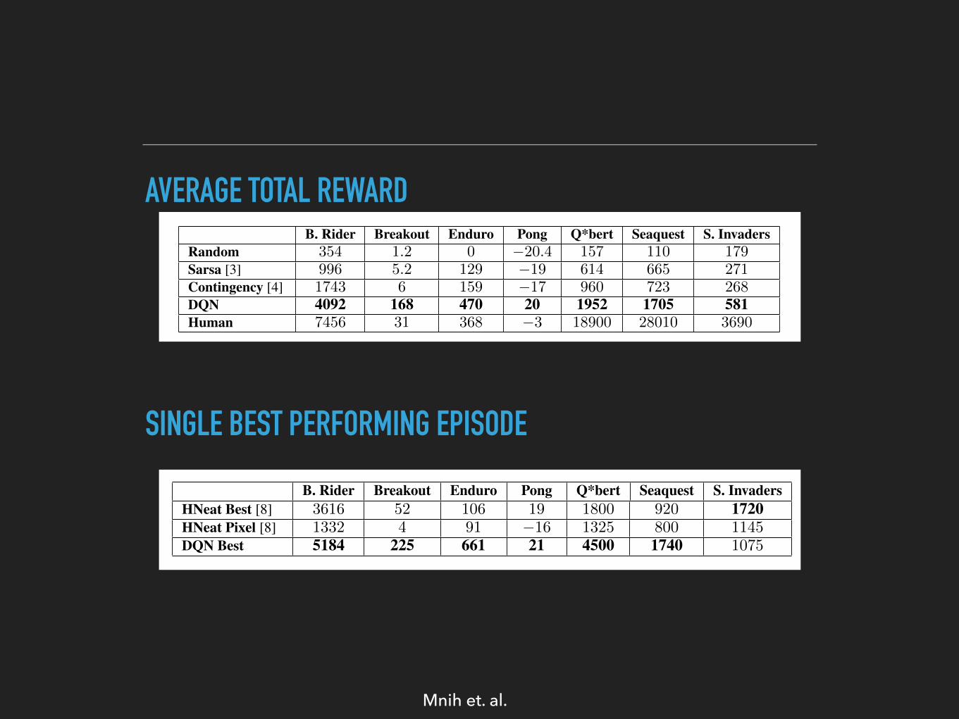
AVERAGE TOTAL REWARD
SINGLE BEST PERFORMING EPISODE
B. Rider Breakout Enduro Pong Q*bert Seaquest S. InvadersRandom 354 1.2 0 �20.4 157 110 179
Sarsa [3] 996 5.2 129 �19 614 665 271
Contingency [4] 1743 6 159 �17 960 723 268
DQN 4092 168 470 20 1952 1705 581Human 7456 31 368 �3 18900 28010 3690
HNeat Best [8] 3616 52 106 19 1800 920 1720HNeat Pixel [8] 1332 4 91 �16 1325 800 1145
DQN Best 5184 225 661 21 4500 1740 1075
Table 1: The upper table compares average total reward for various learning methods by runningan ✏-greedy policy with ✏ = 0.05 for a fixed number of steps. The lower table reports results ofthe single best performing episode for HNeat and DQN. HNeat produces deterministic policies thatalways get the same score while DQN used an ✏-greedy policy with ✏ = 0.05.
types of objects on the Atari screen. The HNeat Pixel score is obtained by using the special 8 colorchannel representation of the Atari emulator that represents an object label map at each channel.This method relies heavily on finding a deterministic sequence of states that represents a successfulexploit. It is unlikely that strategies learnt in this way will generalize to random perturbations;therefore the algorithm was only evaluated on the highest scoring single episode. In contrast, ouralgorithm is evaluated on ✏-greedy control sequences, and must therefore generalize across a widevariety of possible situations. Nevertheless, we show that on all the games, except Space Invaders,not only our max evaluation results (row 8), but also our average results (row 4) achieve betterperformance.
Finally, we show that our method achieves better performance than an expert human player onBreakout, Enduro and Pong and it achieves close to human performance on Beam Rider. The gamesQ*bert, Seaquest, Space Invaders, on which we are far from human performance, are more chal-lenging because they require the network to find a strategy that extends over long time scales.
6 ConclusionThis paper introduced a new deep learning model for reinforcement learning, and demonstrated itsability to master difficult control policies for Atari 2600 computer games, using only raw pixelsas input. We also presented a variant of online Q-learning that combines stochastic minibatch up-dates with experience replay memory to ease the training of deep networks for RL. Our approachgave state-of-the-art results in six of the seven games it was tested on, with no adjustment of thearchitecture or hyperparameters.
References
[1] Leemon Baird. Residual algorithms: Reinforcement learning with function approximation. InProceedings of the 12th International Conference on Machine Learning (ICML 1995), pages30–37. Morgan Kaufmann, 1995.
[2] Marc Bellemare, Joel Veness, and Michael Bowling. Sketch-based linear value function ap-proximation. In Advances in Neural Information Processing Systems 25, pages 2222–2230,2012.
[3] Marc G Bellemare, Yavar Naddaf, Joel Veness, and Michael Bowling. The arcade learningenvironment: An evaluation platform for general agents. Journal of Artificial Intelligence
Research, 47:253–279, 2013.
[4] Marc G Bellemare, Joel Veness, and Michael Bowling. Investigating contingency awarenessusing atari 2600 games. In AAAI, 2012.
[5] Marc G. Bellemare, Joel Veness, and Michael Bowling. Bayesian learning of recursively fac-tored environments. In Proceedings of the Thirtieth International Conference on Machine
Learning (ICML 2013), pages 1211–1219, 2013.
8
Mnih et. al.
DQN PERFORMANCE
see Fig. 3, Supplementary Discussion and Extended Data Table 2). Inadditional simulations (see Supplementary Discussion and ExtendedData Tables 3 and 4), we demonstrate the importance of the individualcore components of the DQN agent—the replay memory, separate targetQ-network and deep convolutional network architecture—by disablingthem and demonstrating the detrimental effects on performance.
We next examined the representations learned by DQN that under-pinned the successful performance of the agent in the context of the gameSpace Invaders (see Supplementary Video 1 for a demonstration of theperformance of DQN), by using a technique developed for the visual-ization of high-dimensional data called ‘t-SNE’25 (Fig. 4). As expected,the t-SNE algorithm tends to map the DQN representation of percep-tually similar states to nearby points. Interestingly, we also found instancesin which the t-SNE algorithm generated similar embeddings for DQNrepresentations of states that are close in terms of expected reward but
perceptually dissimilar (Fig. 4, bottom right, top left and middle), con-sistent with the notion that the network is able to learn representationsthat support adaptive behaviour from high-dimensional sensory inputs.Furthermore, we also show that the representations learned by DQNare able to generalize to data generated from policies other than itsown—in simulations where we presented as input to the network gamestates experienced during human and agent play, recorded the repre-sentations of the last hidden layer, and visualized the embeddings gen-erated by the t-SNE algorithm (Extended Data Fig. 1 and SupplementaryDiscussion). Extended Data Fig. 2 provides an additional illustration ofhow the representations learned by DQN allow it to accurately predictstate and action values.
It is worth noting that the games in which DQN excels are extremelyvaried in their nature, from side-scrolling shooters (River Raid) to box-ing games (Boxing) and three-dimensional car-racing games (Enduro).
Montezuma's RevengePrivate Eye
GravitarFrostbiteAsteroids
Ms. Pac-ManBowling
Double DunkSeaquest
VentureAlien
Amidar
River RaidBank Heist
Zaxxon
CentipedeChopper Command
Wizard of WorBattle Zone
AsterixH.E.R.O.
Q*bertIce Hockey
Up and DownFishing Derby
EnduroTime Pilot
FreewayKung-Fu Master
TutankhamBeam Rider
Space InvadersPong
James BondTennis
KangarooRoad Runner
AssaultKrull
Name This GameDemon Attack
GopherCrazy Climber
AtlantisRobotank
Star GunnerBreakout
BoxingVideo Pinball
At human-level or above
Below human-level
0 100 200 300 400 4,500%500 1,000600
Best linear learner
DQN
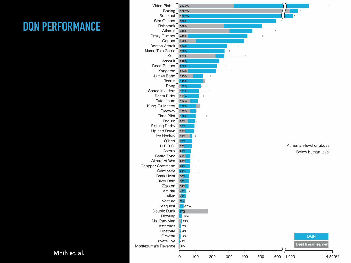
Figure 3 | Comparison of the DQN agent with the best reinforcementlearning methods15 in the literature. The performance of DQN is normalizedwith respect to a professional human games tester (that is, 100% level) andrandom play (that is, 0% level). Note that the normalized performance of DQN,expressed as a percentage, is calculated as: 100 3 (DQN score 2 random playscore)/(human score 2 random play score). It can be seen that DQN
outperforms competing methods (also see Extended Data Table 2) in almost allthe games, and performs at a level that is broadly comparable with or superiorto a professional human games tester (that is, operationalized as a level of75% or above) in the majority of games. Audio output was disabled for bothhuman players and agents. Error bars indicate s.d. across the 30 evaluationepisodes, starting with different initial conditions.
LETTER RESEARCH
2 6 F E B R U A R Y 2 0 1 5 | V O L 5 1 8 | N A T U R E | 5 3 1
Macmillan Publishers Limited. All rights reserved©2015
Mnih et. al.

TEXT
BROADMIND LEARNS OPTIMAL STRATEGY
https://www.youtube.com/watch?v=rbsqaJwpu6A
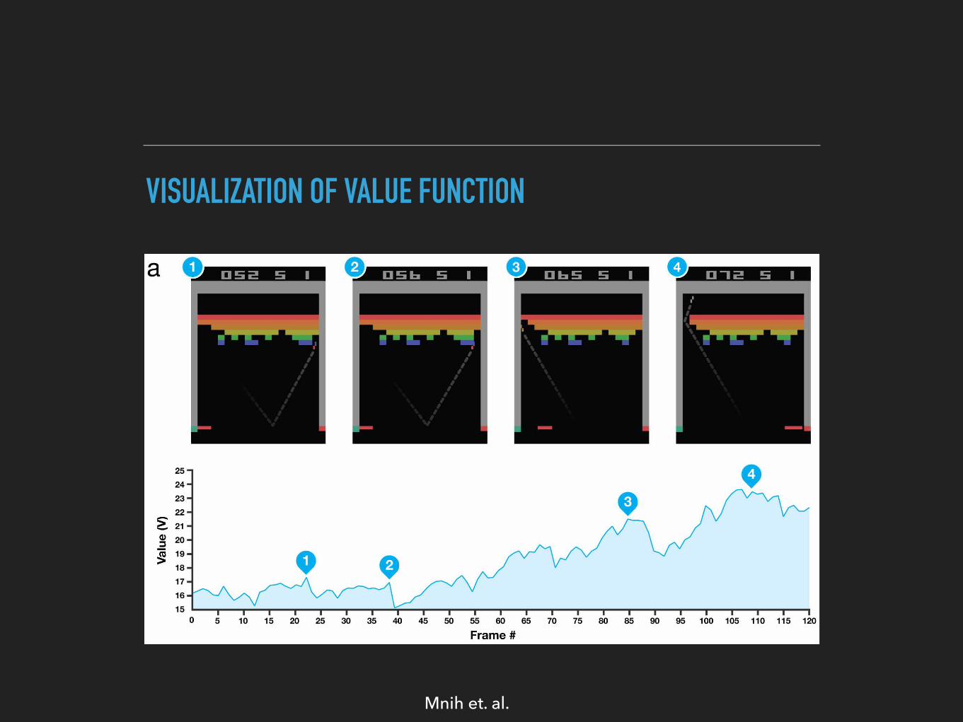
VISUALIZATION OF VALUE FUNCTION
Extended Data Figure 2 | Visualization of learned value functions on twogames, Breakout and Pong. a, A visualization of the learned value function onthe game Breakout. At time points 1 and 2, the state value is predicted to be ,17and the agent is clearing the bricks at the lowest level. Each of the peaks inthe value function curve corresponds to a reward obtained by clearing a brick.At time point 3, the agent is about to break through to the top level of bricks andthe value increases to ,21 in anticipation of breaking out and clearing alarge set of bricks. At point 4, the value is above 23 and the agent has brokenthrough. After this point, the ball will bounce at the upper part of the bricksclearing many of them by itself. b, A visualization of the learned action-valuefunction on the game Pong. At time point 1, the ball is moving towards thepaddle controlled by the agent on the right side of the screen and the values of
all actions are around 0.7, reflecting the expected value of this state based onprevious experience. At time point 2, the agent starts moving the paddletowards the ball and the value of the ‘up’ action stays high while the value of the‘down’ action falls to 20.9. This reflects the fact that pressing ‘down’ would leadto the agent losing the ball and incurring a reward of 21. At time point 3,the agent hits the ball by pressing ‘up’ and the expected reward keeps increasinguntil time point 4, when the ball reaches the left edge of the screen and the valueof all actions reflects that the agent is about to receive a reward of 1. Note,the dashed line shows the past trajectory of the ball purely for illustrativepurposes (that is, not shown during the game). With permission from AtariInteractive, Inc.
LETTER RESEARCH
Macmillan Publishers Limited. All rights reserved©2015
Mnih et. al.

STRENGTHS AND WEAKNESSES
‣Good at
‣Quick-moving, complex, short-horizon games
‣Semi-independent trails within the game
‣Negative feedback on failure
‣Pinball
‣Bad at:
‣ long-horizon games that don’t converge
‣Any “walking around” game
‣ Pac-Man
Source: Nikolai Yakovenko
TEXT
FAILURE CASES
▸ Montezuma’s revenge
▸ Single reward at the end of the level. No intermediate rewards
▸ Worldly knowledge helps humans play these games relatively easily.
▸ https://www.youtube.com/watch?v=1rwPI3RG-lU
JUERGEN SCHMIDHUBER’S TEAM
Evolving Large-Scale Neural Networks for Vision-Based Reinforcement Learning
▸ Evolutionary Computation based deep NN for RL
▸ Learns to play a car-racing video game
▸ No pre-training or hand-coding of features
▸ Video

RELATED TOPICS/PAPERS
▸ Universal Value Function Approximators, DeepMind
▸ http://jmlr.org/proceedings/papers/v37/schaul15.pdf
‣ Deep Learning for Real-Time Atari Game Play Using Offline Monte-Carlo Tree Search Planning , UMich
‣ http://papers.nips.cc/paper/5421-deep-learning-for-real-time-atari-game-play-using-offline-monte-carlo-tree-search-planning
‣ On Learning to Think: Algorithmic Information Theory for Novel Combinations of Reinforcement Learning Controllers and Recurrent Neural World Models, Juergen Schmidhuber ‣ http://arxiv.org/abs/1511.09249

NEURAL NETWORK VISION FOR ROBOT DRIVING
DEAN POMERLEAU

ALVINN - AUTONOMOUS DRIVING SYSTEM
▸ ALVINN has successfully driven autonomously at speeds of up to 70 mph, and for distances of over 90 miles on a public highway north of Pittsburgh.
▸ Multiple NNs trained to handle: single lane dirt roads, single lane paved bike paths, two lane suburban neighborhood streets, and lined two lane highways.
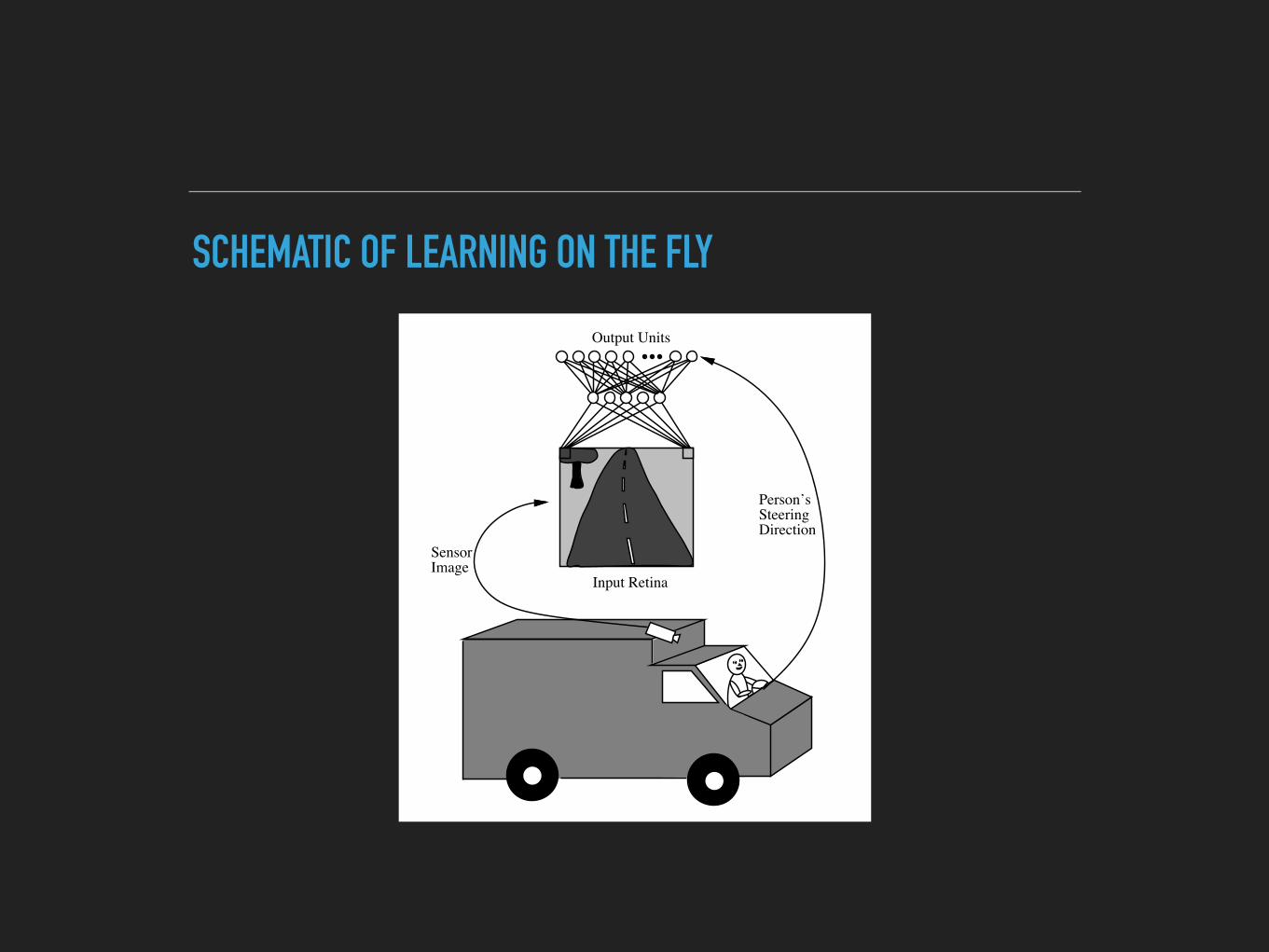
Input Retina
Output Units
Person’sSteeringDirection
SensorImage
SCHEMATIC OF LEARNING ON THE FLY
Sharp Left
SharpRight
4 Hidden Units
30 Output Units
30x32 Sensor Input Retina
Straight Ahead
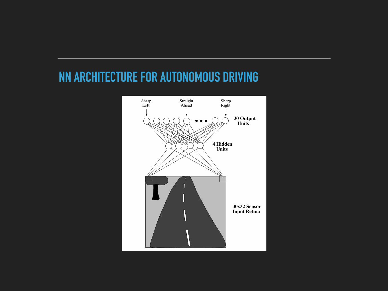
NN ARCHITECTURE FOR AUTONOMOUS DRIVING
ARCHITECTURE
▸ 1-hidden layer NN.
▸ Input layer contains 960 neurons.
▸ 1 hidden layer containing 4 neurons.
▸ Output layer contains 30 neurons.
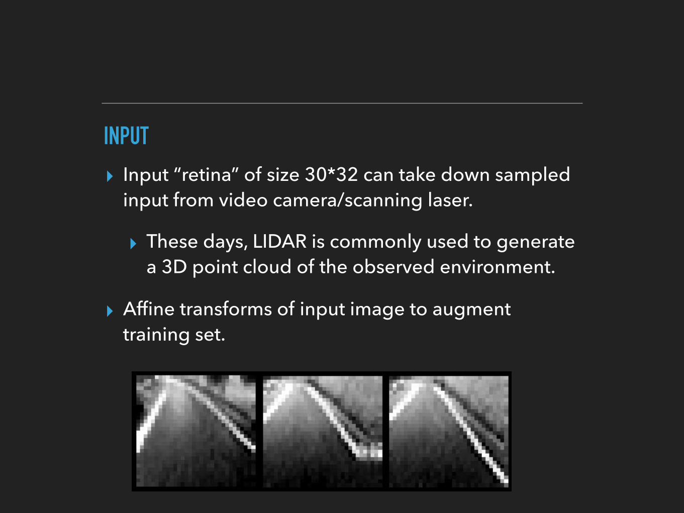
INPUT
▸ Input “retina” of size 30*32 can take down sampled input from video camera/scanning laser.
▸ These days, LIDAR is commonly used to generate a 3D point cloud of the observed environment.
▸ Affine transforms of input image to augment training set.
Original Extrapolation Scheme
Improved Extrapolation Scheme
Camera
OriginalField of View
OriginalVehiclePosition
Transformed Vehicle Position
TransformedField of View
A
C
B
RoadBoundaries
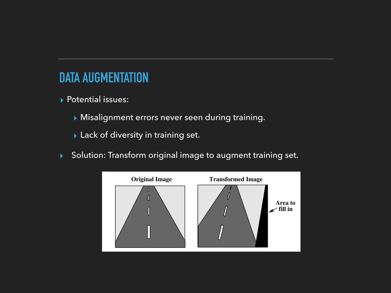
DATA AUGMENTATION▸ Potential issues:
▸ Misalignment errors never seen during training.
▸ Lack of diversity in training set.
Original Image Transformed Image
Area to fill in
▸ Solution: Transform original image to augment training set.

Original Extrapolation Scheme
Improved Extrapolation Scheme
Camera
OriginalField of View
OriginalVehiclePosition
Transformed Vehicle Position
TransformedField of View
A
C
B
RoadBoundaries
EXTRAPOLATION
OUTPUT
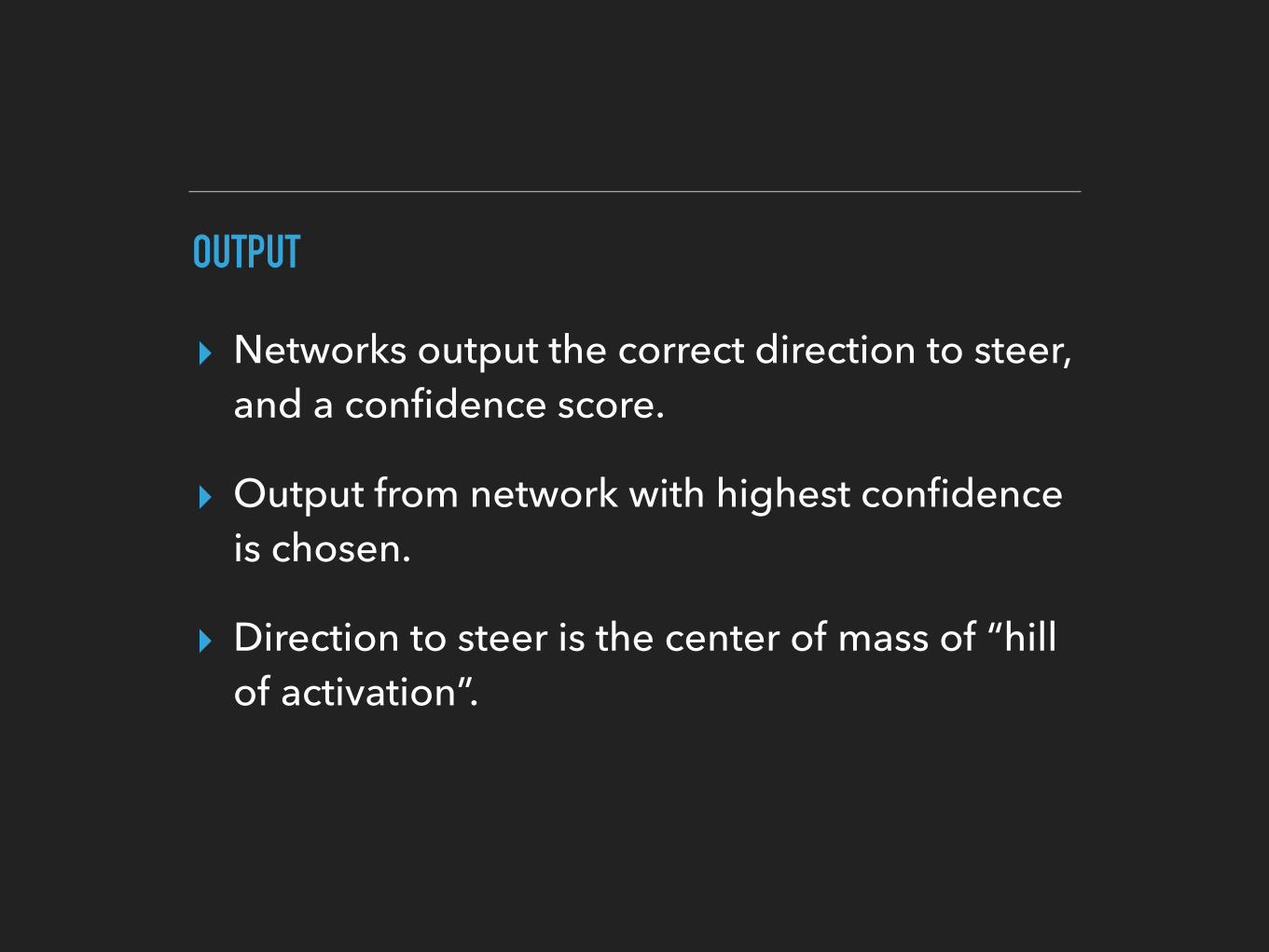
▸ Networks output the correct direction to steer, and a confidence score.
▸ Output from network with highest confidence is chosen.
▸ Direction to steer is the center of mass of “hill of activation”.
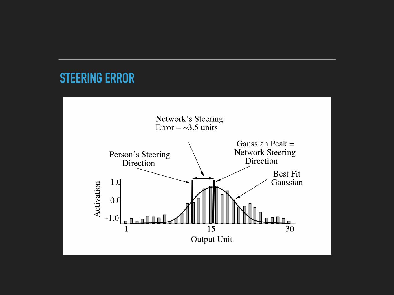
Best FitGaussian
Gaussian Peak =Network Steering Direction
Person’s Steering Direction
Network’s SteeringError = ~3.5 units
Act
ivat
ion 1.0
0.0
-1.01 15 30
Output Unit
STEERING ERROR
TRAINING
▸ Original sensor image is shifted and rotated to create 14 training exemplars.
▸ Buffer of 200 exemplar patterns used to train the network.
▸ Each exemplar is replaced with another with a constant probability to ensure diversity.
▸ 2.5sec per training cycle. Total training time = 4 min.
150
100
50
0
-50
-100
-150
0 25 50 75 100
Distance Travelled (meters)
Disp
lace
men
t fro
m R
oad
Cen
ter
(cm
)
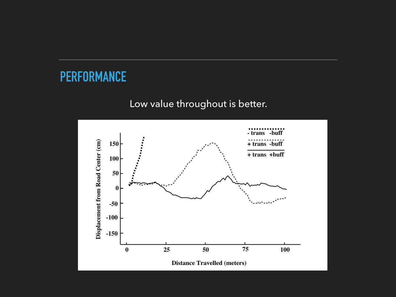
- trans -buff
+ trans -buff
+ trans +buff
PERFORMANCE
Low value throughout is better.

ALVINN
▸ ALVINN (1995)
▸ https://www.youtube.com/watch?v=ilP4aPDTBPE

TAKEAWAY
▸ Creating AGI is hard.
▸ RNNAIs, Memory Networks + RL etc. promise an exciting future
▸ Tangible first step.

THANK YOU!