University of Tartu

Faculty of Mathematics and Computer Science

Institute of Computer Science

Kristjan Korjus, Ilya Kuzovkin, Ardi Tampuu, Taivo Pungas

Replicating the Paper “Playing Atari withDeep Reinforcement Learning”[MKS+13]

Technical Report

MTAT.03.291 Introduction to Computational Neuroscience

Tartu 2014

Contents

Introduction 3

1 Overview of the system 4

1.1 The task . . . . . . . . . . . . . . . . . . . . . . . . . . . . . . . . . . . . 4

1.2 Reinforcement learning . . . . . . . . . . . . . . . . . . . . . . . . . . . . 4

1.2.1 Exploration-exploitation . . . . . . . . . . . . . . . . . . . . . . . 4

1.3 Neural network . . . . . . . . . . . . . . . . . . . . . . . . . . . . . . . . 5

1.4 Learning process . . . . . . . . . . . . . . . . . . . . . . . . . . . . . . . 5

2 Components of the system 7

2.1 Launching and communicating with ALE . . . . . . . . . . . . . . . . . . 7

2.2 Convolutional neural network . . . . . . . . . . . . . . . . . . . . . . . . 7

2.3 Q-learning . . . . . . . . . . . . . . . . . . . . . . . . . . . . . . . . . . . 9

2.4 Root Mean Squares of gradients (RMSProp) . . . . . . . . . . . . . . . . 10

2.4.1 Stochastic gradient descent . . . . . . . . . . . . . . . . . . . . . . 10

2.4.2 RMSProp . . . . . . . . . . . . . . . . . . . . . . . . . . . . . . . 10

3 Implementation details 11

3.1 Atari Learning Environment . . . . . . . . . . . . . . . . . . . . . . . . . 11

3.2 Preprocessing . . . . . . . . . . . . . . . . . . . . . . . . . . . . . . . . . 11

3.3 Memory . . . . . . . . . . . . . . . . . . . . . . . . . . . . . . . . . . . . 12

3.4 Neural network . . . . . . . . . . . . . . . . . . . . . . . . . . . . . . . . 12

3.5 Computing on GPU . . . . . . . . . . . . . . . . . . . . . . . . . . . . . 12

3.6 Running instructions . . . . . . . . . . . . . . . . . . . . . . . . . . . . . 12

4 Results 13

4.1 Performance measures . . . . . . . . . . . . . . . . . . . . . . . . . . . . 13

4.2 Comparison to human player . . . . . . . . . . . . . . . . . . . . . . . . . 13

4.3 Comparison to the original paper . . . . . . . . . . . . . . . . . . . . . . 13

4.4 Applications and future usage . . . . . . . . . . . . . . . . . . . . . . . . 13

Bibliography 14

Introduction

In recent years the popularity of the method called deep learning [Hin07] has increasednoticeably in the machine learning community. Deep learning was successfully applied tospeech recognition[DYDA12] and many other tasks in machine learning[DHK13]. In all thesestudies the performance of the resulting system was better than other machine learningmethods were able to achieve so far.

The core of the deep learning method is an artificial neural network. One of the proper-ties, which gives this family of learning algorithms a special place, is the ability to extract“meaningful” (from a human perspective) concepts from the data by combining the fea-tures based on the structure of the data. The extracted concepts sometimes have clearinterpretation and that makes us feel as if the machine has indeed learned something.Here we step into the realm of artificial intelligence, the possibility of which never stopsto fascinate our minds.

A recent work, which brings together deep learning and artificial intelligence is a pa-per “Playing Atari with Deep Reinforcement Learning”[MKS+13] published by DeepMind1

company. The paper describes a system that combines deep learning methods and rein-forcement learning in order to create a system that is able to learn how to play simplecomputer games. It is worth mentioning that the system has access only to the visualinformation (screen of the game) and the scores. Based on these two inputs the systemlearns to understand which moves are good and which are bad depending on the situationon the screen. Notice that a human player uses exactly same information to evaluate herperformance and adapt her playing strategy. The reported result shows that the systemwas able to master several different games and play some of them better than a humanplayer.

This result can be seen as a step towards truly intelligent machines and thus it fascinatesus. The goal of this project is to create an open-source analogue of such a system usingthe description provided in the paper.

1http://deepmind.com

3

1 Overview of the system

Before we go into the details, let us describe the overall architecture of the system andshow how the building blocks are put together.

1.1 The task

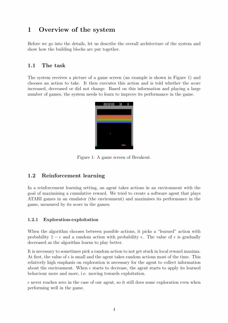
The system receives a picture of a game screen (an example is shown in Figure 1) andchooses an action to take. It then executes this action and is told whether the scoreincreased, decreased or did not change. Based on this information and playing a largenumber of games, the system needs to learn to improve its performance in the game.

Figure 1: A game screen of Breakout.

1.2 Reinforcement learning

In a reinforcement learning setting, an agent takes actions in an environment with thegoal of maximising a cumulative reward. We tried to create a software agent that playsATARI games in an emulator (the environment) and maximises its performance in thegame, measured by its score in the games.

1.2.1 Exploration-exploitation

When the algorithm chooses between possible actions, it picks a “learned” action withprobability 1 − ε and a random action with probability ε. The value of ε is graduallydecreased as the algorithm learns to play better.

It is necessary to sometimes pick a random action to not get stuck in local reward maxima.At first, the value of ε is small and the agent takes random actions most of the time. Thisrelatively high emphasis on exploration is necessary for the agent to collect informationabout the environment. When ε starts to decrease, the agent starts to apply its learnedbehaviour more and more, i.e. moving towards exploitation.

ε never reaches zero in the case of our agent, so it still does some exploration even whenperforming well in the game.

4

1.3 Neural network

The system uses a neural network to assign an expected reward value to each possibleaction. The input to the network at any time point consists of the last four preprocessedgame screens the system received. This input is then passed through three successivehidden layers to the output layer.

The output layer has one node for each possible action and the activation of those nodesindicates the expected reward from each of the possible actions - here, the action withthe highest expected reward is selected for execution.

1.4 Learning process

Under the fancy word “neural network” hides a quite simple idea: a bunch of nodes(neurons), each of them having some input to perform a computation on and an outputwhere the result of the computation will be sent to, are connected to each other. Eachconnection has a weight, which regulates how much one neuron can affect another. Thevery first layer of the network is usually called the input layer. This is the place where weinject a data sample. Next to the input layer the network has several trickily connectedhidden layers. And the last layer is an output layer, it gives us the final piece of informa-tion we wanted to know about the data sample we fed into the network. The resultingstructure can be very complex, but the building blocks are always the same: neurons andconnections between them.

We, as the builders of the system, usually know what we want it do: that is for each datasample we know what the final output should look like. Now the “smart” neural networkis the one able to produce the output we expect, the “naive” network is the one which isnot. The only thing that differs in those two are the weights on the connections betweenthe nodes. By changing them in accordance with our final goal the network goes frombeing “naive” to being “smart”. This process in general in known as learning.

To explain the concept of learning to the machine we introduce the notion of cost function(or loss function) which we will denote by L. Given the parameters of the network thisfunction goes over the data samples, computes the outputs, compares these outputs withthe expected ones and calculates how big is the error the system makes. The learningprocess can be represented as the process of minimizing the cost function.

The obvious way to minimize a function is to try out all possible inputs to find theminimal output. Unfortunately the number of possible input is unfeasibly large. How todo it is a big question not only for our system. The whole brach on computer sciencecalled optimization is dealing with this issue. One of the most popular technique used inthis area is called gradient descent.

The idea of gradient descent is rather trivial: at each iteration of the learning algorithm itmakes a small step in the “direction” which makes the value of the loss function smaller.Thus by making enough steps the algorithm will reach an optimum: a place from where astep in any direction will only increase the value of the loss function. Once this optimumis found we say that the learning has finished and the system is now as smart as it canbe. It might happen that the optimum we found is not the best one (local optimum),and there are bunch of techniques (for example Monte Carlo methods) to find the global

5

optimum, but we will not dwell into this right now.

Gradient descent uses the gradient (multidimensional derivative) as it’s core:

1. Let the current configuration of the system be w0

2. Compute the derivative (gradient) of the loss function at this point L(w0)

3. Look at the derivative with respect to each element (w1, . . . , wn) = w0 and:

(a) If the derivative is 0 then we should not touch this parameter of our system

(b) Otherwise move one step in the direction opposite to the derivative (positiveslope – decrease the parameter, negative slope – increase the parameter)

4. Repeat starting from the step 2. until the derivatives with respect to all parametersof the system are zeros (or close to zeros)

Once this process is complete, we believe that our system has reached the optimal state:its parameters are configures in such way that it will give optimal performance on thedataset we have. In our system we will use variation of the idea of gradient descent calledRMSProp, you will read about it later.

6

2 Components of the system

In this section we intend to describe all the key components of the system in detail.This description should reflect all the choices we made, justify them and explain how thecomponents work.

2.1 Launching and communicating with ALE

Just as we, humans, exchange information with a computer game by seeing the computerscreen (input) and pressing the keys (output actions), the system needs to communicatewith the Arcade Learning Environment that hosts the game.

Communication with ALE is achieved using two first-in-first-out (FIFO) pipes whichmust be created before ALE is launched. We create the pipes and launch ALE usingthe os package of Python. The parameters given to ALE at execution must specify theway we want to communicate with ALE (FIFO pipes) and the location of the binary filecontaining the game to run (Breakout). In addition, we specify that we want ALE toreturn unencoded images, that only every 4th frame should be sent to us and whetherthe game window should be made visible.

The actual communication starts with a handshake phase, where we define the desiredinputs (screen image and episode information) and ALE responds by informing us aboutthe dimensions of the image. Thereafter the conversation between ALE and our agentconsists in reading and deciphering inputs from FIFO in pipe and sending the chosenactions back through FIFO out pipe. The information is read from pipes as one longString, so deciphering is needed (cutting the input and converting the pieces into appro-priate types). Similarly, the chosen action has to be transformed to an output string ofspecific format. If a game is lost, a specific “reset” signal is sent to start the next game.When the desired number of games has been played, the communication with ALE canbe terminated by closing the communication pipes.

2.2 Convolutional neural network

Our system receives 4×84×84 pixel values as input. In order to find relevant informationfrom these four 84×84 images, we use convolutional neural networks (CNN)[LB95]. CNNsare a specific type of neural network that are particularly adapted to extracting featuresfrom images.

Unlike restricted Boltzmann machines (RBMs) that see their input as an 1D vector,a CNN treats the input images as 2D objects. These 2D matrices of pixel values areconvolved with linear filters to obtain the activities of the next layer. For example, ourfirst hidden layer is generated by convolving our images with sixteen different 8×8 filters,using a step of 4 pixels. This means that for each of the 16 different filters, we first takethe top left 8× 8 values of an image and linearly combine them with the filter, obtainingas a result one activity value. We then move 4 pixels to the right and multiply another

7

8 × 8 area from the image with the same filter. When reaching the right edge of theimage, we start again from the left, only 4 pixels lower. There are 8 · 8 · 4 weights in afilter of this kind and the same weights (the same filter) is applied at different positionsof the image, as described.

Each linear combination yields one activity value, so convolving an 84 × 84 image withan 8 × 8 filter with step 4 produces 20 × 20 topologically arranged values. As we apply16 different filters, we end up with 16 · 20 · 20 nodes in the first hidden layer of ourconvolutional network.

An attentive reader will notice that our input consists of 4 images, not one. This meansthat each of our filters contains four weight matrices of size 8 × 8. The images will beconvolved with the corresponding 8× 8 matrix and the calculated activities are summed,so we end up with 16 · 20 · 20 values as before.

Last but not least, a linear rectifier is applied to the activity values, setting all negativevalues to 0.

The obtained sixteen 20× 20 feature maps are thereafter convolved with 32 4× 4 filters.Using a step of 2, this yields 32 × 9 × 9 activity values in the second hidden layer. Asbefore, the filters are not 2-dimensional, instead they have 16× 4× 4 values.

With these two convolutional layers we have reduced the number of nodes from 4×84×84to 32× 9× 9. Functionally, after training the system we expect the nodes of the secondhidden layer to represent spatiotemporal patterns relevant for successfully playing thegame.

8

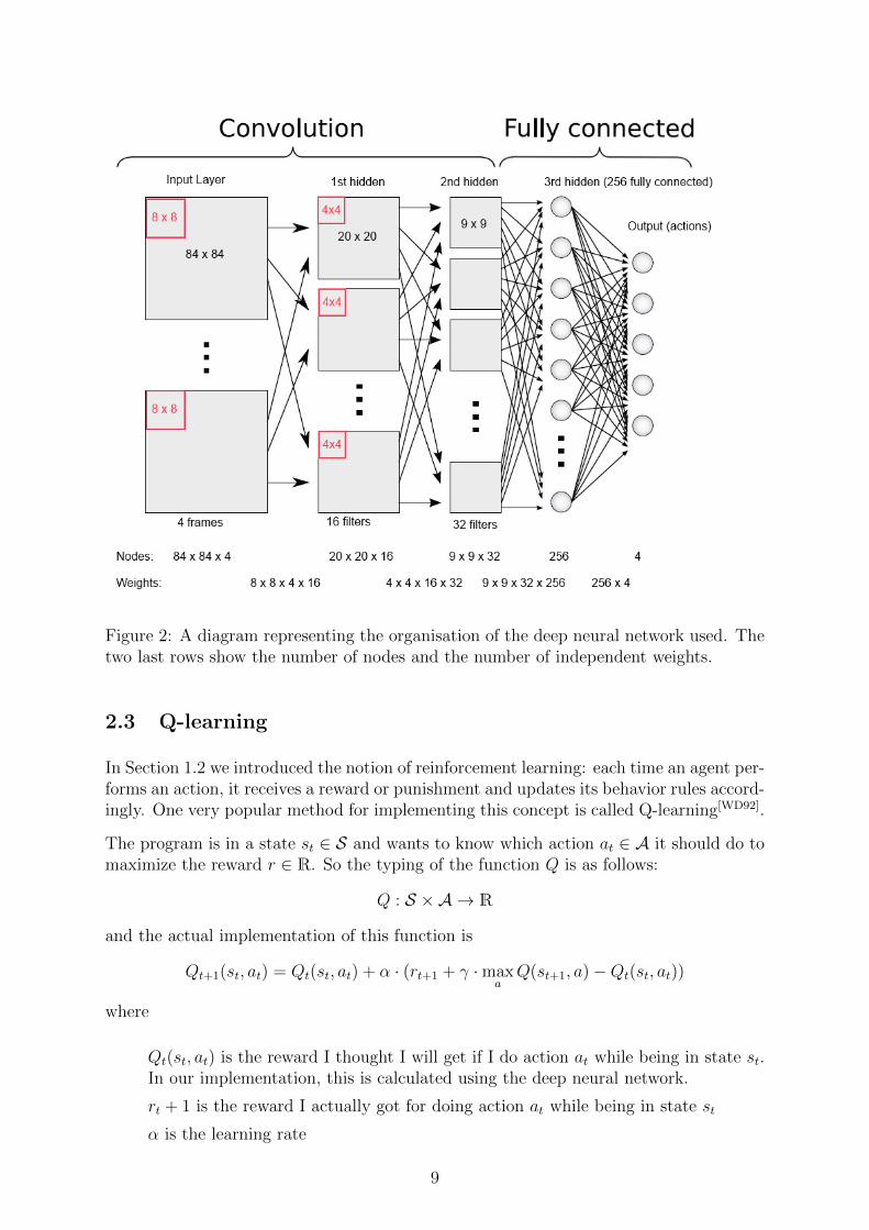
Figure 2: A diagram representing the organisation of the deep neural network used. Thetwo last rows show the number of nodes and the number of independent weights.

2.3 Q-learning

In Section 1.2 we introduced the notion of reinforcement learning: each time an agent per-forms an action, it receives a reward or punishment and updates its behavior rules accord-ingly. One very popular method for implementing this concept is called Q-learning[WD92].

The program is in a state st ∈ S and wants to know which action at ∈ A it should do tomaximize the reward r ∈ R. So the typing of the function Q is as follows:

Q : S ×A → R

and the actual implementation of this function is

Qt+1(st, at) = Qt(st, at) + α · (rt+1 + γ ·maxaQ(st+1, a)−Qt(st, at))

where

Qt(st, at) is the reward I thought I will get if I do action at while being in state st.In our implementation, this is calculated using the deep neural network.

rt + 1 is the reward I actually got for doing action at while being in state st

α is the learning rate

9

γ is a discount factor which says how much should I take into consideration thefuture rewards along this path

maxaQ(st+1, a) is what I think will be the best reward available from the next state(future reward)

2.4 Root Mean Squares of gradients (RMSProp)

In Section 1.4 we have seen the logic of gradient descent update procedure. There are,however, problems with this approach. One of them is that once you have establishedand update vector u you might notice that for some components ui = ∂L(w)

∂wiit proposes

huge changes and tiny changes for the others. It might be not very reasonable to usethe same learning µ rate for all components. The idea of RMSProp is to come up with aseparate learning rate µi for each of the components ui.

If you can use all of your data to estimate the direction of the gradient, then you cancope with this problem by just using sign of the gradient sign(∂L(w)

∂wi). This will ensure

that all components of the gradient are treated equally. This approach is called rprop.However we do not have the luxury of using all the data points in our loss function L: itwould take too much time. This is where the idea of stochastic gradient descent comesinto play.

2.4.1 Stochastic gradient descent

As you know, if you have a set of differentiable functions, then the sum of these functions isalso differentiable and the derivative of this function is equal to the sum of the derivativesof these functions:

∇f(w,x) =∑∇g(w,xk)

where x is a set of data samples and xk is one data sample. This fact allows us to take asample from the dataset, compute updates u on it and then repeat this several time. Atthe end of the day it will produce the same results as if we had performed the gradientdescent on the whole dataset at once.

Unfortunately rprop does not work with small sets of subsamples[TH12] (minibatches).Although the blunt simplification of taking the gradient sign instead of the value workswhen we use the whole dataset (because it effectively converges to the average value ofthe magnitude of the update) it does not work on small random subsamples: there wecould easily obtain an update which is too large compared to what we would like to have.The next build-up on top of the rprop idea is called rmsprop and deals with that issue.

2.4.2 RMSProp

When we average the results obtained using rprop method we divide by the magnitude ofthe gradient. RMSProp proposes to keep track of previous gradients and divide updatesnot by the current magnitude, but the average magnitude over the last several updates(minibatches). This will allow to modify each component ui according to its previousmagnitudes, preventing from taking it into account with too large or too small weight.

10

3 Implementation details

The prototype of the system is built using Python 2.7 with heavy usage of theano[BBB+10]

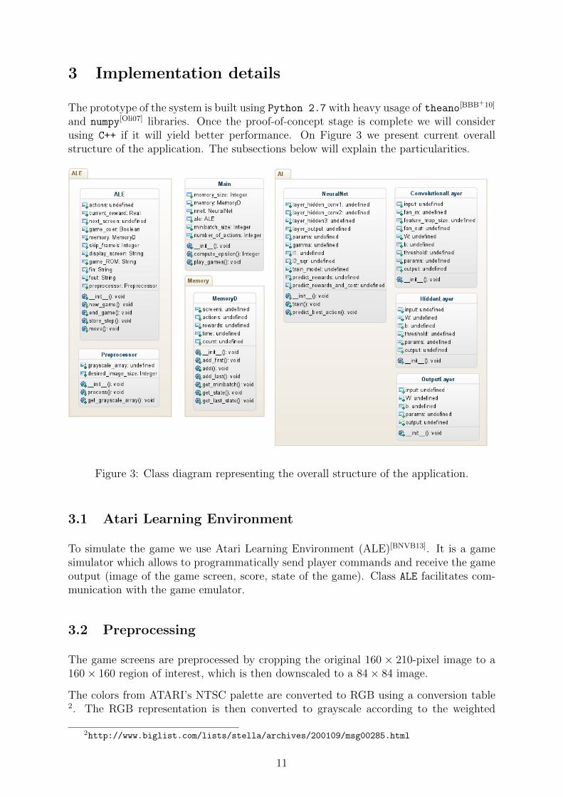
and numpy[Oli07] libraries. Once the proof-of-concept stage is complete we will considerusing C++ if it will yield better performance. On Figure 3 we present current overallstructure of the application. The subsections below will explain the particularities.

Figure 3: Class diagram representing the overall structure of the application.

3.1 Atari Learning Environment

To simulate the game we use Atari Learning Environment (ALE)[BNVB13]. It is a gamesimulator which allows to programmatically send player commands and receive the gameoutput (image of the game screen, score, state of the game). Class ALE facilitates com-munication with the game emulator.

3.2 Preprocessing

The game screens are preprocessed by cropping the original 160 × 210-pixel image to a160× 160 region of interest, which is then downscaled to a 84× 84 image.

The colors from ATARI’s NTSC palette are converted to RGB using a conversion table2. The RGB representation is then converted to grayscale according to the weighted

2http://www.biglist.com/lists/stella/archives/200109/msg00285.html

11

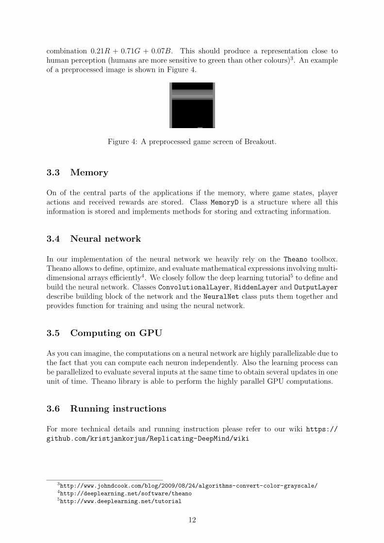
combination 0.21R + 0.71G + 0.07B. This should produce a representation close tohuman perception (humans are more sensitive to green than other colours)3. An exampleof a preprocessed image is shown in Figure 4.

Figure 4: A preprocessed game screen of Breakout.

3.3 Memory

On of the central parts of the applications if the memory, where game states, playeractions and received rewards are stored. Class MemoryD is a structure where all thisinformation is stored and implements methods for storing and extracting information.

3.4 Neural network

In our implementation of the neural network we heavily rely on the Theano toolbox.Theano allows to define, optimize, and evaluate mathematical expressions involving multi-dimensional arrays efficiently4. We closely follow the deep learning tutorial5 to define andbuild the neural network. Classes ConvolutionalLayer, HiddenLayer and OutputLayer

describe building block of the network and the NeuralNet class puts them together andprovides function for training and using the neural network.

3.5 Computing on GPU

As you can imagine, the computations on a neural network are highly parallelizable due tothe fact that you can compute each neuron independently. Also the learning process canbe parallelized to evaluate several inputs at the same time to obtain several updates in oneunit of time. Theano library is able to perform the highly parallel GPU computations.

3.6 Running instructions

For more technical details and running instruction please refer to our wiki https://

github.com/kristjankorjus/Replicating-DeepMind/wiki

3http://www.johndcook.com/blog/2009/08/24/algorithms-convert-color-grayscale/4http://deeplearning.net/software/theano5http://www.deeplearning.net/tutorial

12

4 Results

At this point of time we can not drive any conclusions about how well the system performor is it functional at all. Before we will be able to estimate that we need to finish thesystem build-up and confirm that all the learning procedures work.

4.1 Performance measures

One possible measure will be to plot the score change over the time. If we will observethat over the time the system is able to score more during fixed-length time window thanbefore, we will have a strong indication that the system is doing something reasonable.

4.2 Comparison to human player

Yet to be performed.

4.3 Comparison to the original paper

Yet to be performed.

4.4 Applications and future usage

We believe that the technique used in this system allows to solve wide variety of machinelearning tasks. It will be interesting to test the system on machine learning benchmarkdatasets.

13

References

[BBB+10] James Bergstra, Olivier Breuleux, Frederic Bastien, Pascal Lamblin, Raz-van Pascanu, Guillaume Desjardins, Joseph Turian, David Warde-Farley, andYoshua Bengio. Theano: a cpu and gpu math expression compiler. In Pro-ceedings of the Python for scientific computing conference (SciPy), volume 4,2010.

[BNVB13] M. G. Bellemare, Y. Naddaf, J. Veness, and M. Bowling. The arcade learningenvironment: An evaluation platform for general agents. Journal of ArtificialIntelligence Research, 47:253–279, 06 2013.

[DHK13] Li Deng, Geoffrey Hinton, and Brian Kingsbury. New types of deep neural net-work learning for speech recognition and related applications: An overview. InAcoustics, Speech and Signal Processing (ICASSP), 2013 IEEE InternationalConference on, pages 8599–8603. IEEE, 2013.

[DYDA12] George E Dahl, Dong Yu, Li Deng, and Alex Acero. Context-dependent pre-trained deep neural networks for large-vocabulary speech recognition. Audio,Speech, and Language Processing, IEEE Transactions on, 20(1):30–42, 2012.

[Hin07] Geoffrey E Hinton. Learning multiple layers of representation. Trends incognitive sciences, 11(10):428–434, 2007.

[LB95] Yann LeCun and Yoshua Bengio. Convolutional networks for images, speech,and time series. The handbook of brain theory and neural networks, 3361,1995.

[MKS+13] Volodymyr Mnih, Koray Kavukcuoglu, David Silver, Alex Graves, IoannisAntonoglou, Daan Wierstra, and Martin Riedmiller. Playing atari with deepreinforcement learning. arXiv preprint arXiv:1312.5602, 2013.

[Oli07] Travis E Oliphant. Python for scientific computing. Computing in Science &Engineering, 9(3):10–20, 2007.

[TH12] T Tieleman and G Hinton. Lecture 6.5-rmsprop: Divide the gradient by arunning average of its recent magnitude. COURSERA: Neural Networks forMachine Learning, 4, 2012.

[WD92] Christopher JCH Watkins and Peter Dayan. Q-learning. Machine learning,8(3-4):279–292, 1992.

14