Planning horizons for manpower planning a two level-hierarchical systemCitation for published version (APA):Nuttle, H. L. W., & Wijngaard, J. (1979). Planning horizons for manpower planning a two level-hierarchicalsystem. (Manpower planning reports; Vol. 19). Technische Hogeschool Eindhoven.

Document status and date:Published: 01/01/1979

Document Version:Publisher’s PDF, also known as Version of Record (includes final page, issue and volume numbers)

Please check the document version of this publication:

• A submitted manuscript is the version of the article upon submission and before peer-review. There can beimportant differences between the submitted version and the official published version of record. Peopleinterested in the research are advised to contact the author for the final version of the publication, or visit theDOI to the publisher's website.• The final author version and the galley proof are versions of the publication after peer review.• The final published version features the final layout of the paper including the volume, issue and pagenumbers.Link to publication

General rightsCopyright and moral rights for the publications made accessible in the public portal are retained by the authors and/or other copyright ownersand it is a condition of accessing publications that users recognise and abide by the legal requirements associated with these rights.

• Users may download and print one copy of any publication from the public portal for the purpose of private study or research. • You may not further distribute the material or use it for any profit-making activity or commercial gain • You may freely distribute the URL identifying the publication in the public portal.

If the publication is distributed under the terms of Article 25fa of the Dutch Copyright Act, indicated by the “Taverne” license above, pleasefollow below link for the End User Agreement:www.tue.nl/taverne

Take down policyIf you believe that this document breaches copyright please contact us at:openaccess@tue.nlproviding details and we will investigate your claim.

Download date: 09. Feb. 2022

EINDHOVEN UNIVERSITY OF TECHNOLOGY

Department of Industrial Engineering

Department of Mathematics and Computing Science

)'\0 '5 PLANNING HORIZONS FOR MANPOWER PLANNING IN

A TWO LEVEL-HIERARCHICAL SYSTEM

by

Henry L.W. Nuttle * Jacob Wijngaand **

* North Carolina State University at Raleigh, Department of Industrial Engineering

** Eindhoven University of Technology, Department of Industrial Engineering

1

Planning Horizon Por Manpower Planning In

A Two-Level Hierarchical System

by

Henry L. t-1. Nuttle·

Jacob Wijngaard

Abstract

··' ,·

'

The purpose of manpower planning is to get a better matching between

manpower r~quirement and manpower availability. The difficult part of

manpower planning is to get reliable forecasts for future manpower require-,...

ment. It is important, therefore, to knat-1 what information one needs about

the future to make good decisions now.· How detailed should our kn0t1ledge

of future manpower requirement be and of hm, far in the future? The last

point is directly related to the problem of the planning horizon. This

problem is investigated in this paper for a hierarchical manpower system

t.d.th two grades, recruitment at the bottom and a promotion policy f omu-

lated·in the grade-age (number of years in grade one). There is a goal·

on the total content of the system and a goal on the content of the

second level. These goals may be interpreted as the future requirements.

The penalties for deviations from the goals are assumed ·to be proportional

to these deviations. The only t.,ay to control the system is by recruitment.

For the case where all employees have the same career pattern one

can get rather general results since this problem is almost equivalent to

the case with only one grade. For the more general case it is only pos-

sible to get planning horizon results if conditions are added on the

penalty functions. and. the goal patterns •. The general two-level case

appears to be equivalent to the production-smoothing problem without

inventory with a lcn-1er bound on the difference between the hiring in

two subsequent periods •

... -

-- .- ' • · 1. Introduction

. . . . .

The problem of medium and long tera manpower planning Y. to get

a good match of the future requirementeof personnel and the future

availability of personnel.

The future requirement for personnel in the various categories . .

is determined by the organization activity plans. The future availability

of personnel is determined by the actual population, together with the

policy with respect to rec!Uitment, promotion, job rota.tion, and so on.

The problem is to match requirement and availability as good as possible.

The difficul~y with manpower planning is that all decisions made to . \.

ad~ust availability and requirement to each other have a long lasting

impact on the organization. It is not possible to adjust from year to

year because of, for instance, the following points.

It is difficult to fire people or to move people from one

location to another.

.··; ... ·~· ; .. :

.··· ,. ' ~

- . f: ~ ..

2

- People have (implicit or explicit) career rights; career

possibilities have to remain stable therefore. -·.

-·For many functions one needs people with experience in

the organization and these people are no.t di~ectly

available at the labor market. I ... , "·~ l':•

The difficulty of this long lasting impact of personnel decisions is ,

even more severe because of the fa.ct that it is not possible to get

. good f~ecasts ·for future req~irement. It is difficult to plan more

than five years ahead while the decisions have certainly a longer im---

pact than five years. It is ·extremely important, therefore, to knot'1

how much of the future one has to know to be able to make good. deci-. .

sions n°'·1. So the question is in. the first place, how far in the future

one needs to have information about the requirement. In the second .,

place. how detailed should this information be. The first point is the

problem of choosing the proper planning horizon. The second point has

to do vi.th the level of aggregation. Although these points are related

(longer planning horizon, higher level of aggregation) we will consider . .

here only the planning horizon problem.

In thinking about planni.ng horizons there are two possible points

of view, .the deterministic and the stochastic·. In the deterministic

approach one assumes that it is possible to acquire perfect information

about future. data (in this case future personnel requirement), but that

it is difficult to get this information and that it is important, there-

fore, to know how much information one needs ~o make a good first-period

decision (see, for inst'!lllce, Lundin, Morton [5] and Morton [6] for this

approach in production planning). In the ot~er approach one assumes

·.

..

3

that the forecasts have a given (un)reliability and one considers the - --- - ------ ------

qualf:ty of the planning as f~ction of the horizon (see Baker, Pe_te_rsc:>I!.. __ _

· ~~-r ~0(:8-:_n __ ej~p-~~-:~o!_ ~~~~s·-~approach) •

In this paper we use the deterministic approach. The problem we

consider is a two-level hierarchical system where the only control

possibility is recruitment (only at the lower level) and where promo-

tion depends on grade-age, that is the time spent in the last grade. . .

The system is rather typical for formal organizations (see, for instance,

van der Beek, Verhoeven, Wessels [3]). The only purpose of the decisions

is to minimize the deviation of future (expected) availability from

future requirement (goals) • It 17111 turn, out that it is not possible

for the general two-level case to get good planning horizon results

without making extra assumptions about goal patterns and penalty func-

tion.s. The special, but interesting, case where all employees have

tbe same career pattern is easier since in this case the system is

almost equivalent to a one-level system.

The model is described in more detail in Section 2. Section 3

gives a transformation of the problem which brings it somewhat closer

to the production planning type problems. In Section 4 the one-level

case is considered and in Section 5 the two-level case. Subsection 5.1

gives the special case; subsection 5.2 the general case. Section 6 at •

last gives a discussion of the differences of this problem and a re-. lated production-smoothing problem considered in Aronson, !torten,

Thompson [l] and expla~s why it is not possible to get planning hori-

zon results for the more-level case without making extra assumptions

on goal patterns and penalty functions.

'; Rt.¥ P .. :.;;~~:..,._.Yfohf4":?_*··. ~_.).!!1_.A«,".-j_OO .. #,SJif_..}...__4. ''.·r. -. "'· ·.!.* __ .-.··.J-_?_.,' .. 'r.,.,· ....... .S_£1_._ ..... ::\l_~_?; !£4_ s ... f_,*fa.~¥+.A_:?W5.'.-·.-· ,_}_·*S_.f_ i! ...... ·,_"_ .f9_. •,-,,_;;; ___ e_ ·~t_ ·"· .4&*.·.'· '·'·:·._•;_ ,·.·.· " -k .>p.S.¥lJQ4% !1 Zk.::;;oe 244 -&.I u::;;w;: CJ,.$..,(!& • •. m -. :&?.-.. u•i • .:P.; ™~WU'**""'~ • , -. ~ • ~ <;· ",·"· .. ~· .. :. ···~-:.-r~ ::,_';:.-Jo~ ~--.;~.;..(""·:.:· .•. 'I ·-·:··;_-:.,•·,:;:~:~·-.i:.·'"··.'·•:,7··;· _..·· ·~.·; .. ;

4

2. The Model

Cons~ a linear hierarchical system with 010 grades. The promo­

tion policy is such that people with less than l years of service in

grade ~ (grade-age < l) cannot be promoted to grade 2. The probability

to be promoted for people ld.th l years of service in grade 1, or more

is p. Recruitment is only in grade 1. Promotion as well as recrv.itment

are assumed to take place once a year at a certain fixed date. The

probability to leave the system (turnover) is a, independent of grade

and grade-age. That means ~at the system may be described by a

11arkov-type model with states (1,1), (1,2), ••• ,(l,l.) and (2), where

(l,i) indicates the category of people in grade 1 with grade-age i

(see Figure 1). People recruitec;l in grade l now are assumed to be in

state (1,1) ·during this year. Next year· they enter state (1,2).

level 2

Figure 1

'Ctz5'- a

/

Suppose that the current content is given by the numbers

11>11, w12, ••• ,wl.! and (1)2, let z(t) be the recruitment in year t and

x11Ct), x12Ct), ••• ,xlt(t) and x2Ct) the expected content of the

different categories in year t; then the following equations are · ,.

satisfied

.

xli(O) • wli' x2<g> • w2

and for t .?_ 0 x11Ct+l) • z(t+l)

,.; -~jCt+l) • c1~a>x1j-l (t), j = 2, ••• ,l-1

xli.(t+l) • (l-a)xll-l(t) + (l-a)(l~p)x1,e(t)

x2

(t+l) • (1-a)pxl.l(t) + (1-a) x2 (t)

We assume that there are goals on the future expected content of the

system, in the first place a goal g1(t) on the content of the whole . l

·system at time t, I x1j(t) + x2(t), and in the second place a goal

j•l . g2(t) on the content of the second level, x2(t). The costs of devia-

tions from these goals are assumed to be given by

The only way to control the system and keep it close to the goals is by

choosing the ·&ppropriate recruitment. 'rhe problem we will consider is

to choose recruitment such that the total cost of deviations over a

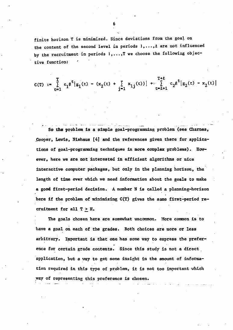
6

finite horizon T is minimized. Since deviations from the goa~ on

the content of the second level in periods 1, ••• ,1 are not influenced

by the recruitment in periods l, ••• ,T we choose the following objec-

tive function:

So the problem is a simple goal-programming problem (see Charnes,

,Cooper, Lewis, Niehaus [4) and the references given there for applica­

tions of goa.1-programm:l.ng techni.ques in more complex problems) • Hcn'f-

ever, here we are not interested in efficient algorithms or nice

interactive computer packages, but only in the planning horizon, the ·

length of time over which we need information about the goals to make

a good first-period decision. A number N is called a planning-horizon

here if the problem of minimizing C(T) gives the same first-period re-

cruitment for all T > N.

The goals chosen here are som~that uncommon. More common is to

have a goal on each of the grades. Both choices are more or less

arbitrary. I~portant is that one has some way to express the pref er-

ence for certain grade contents. Since this study is not a direct

application, but a way to get some insight in the amount of inform.a-

tion required in this type of problem., it is not too important which

.way of representing this preference is chosen.

~·.f.~:;.--... ·-.-

7

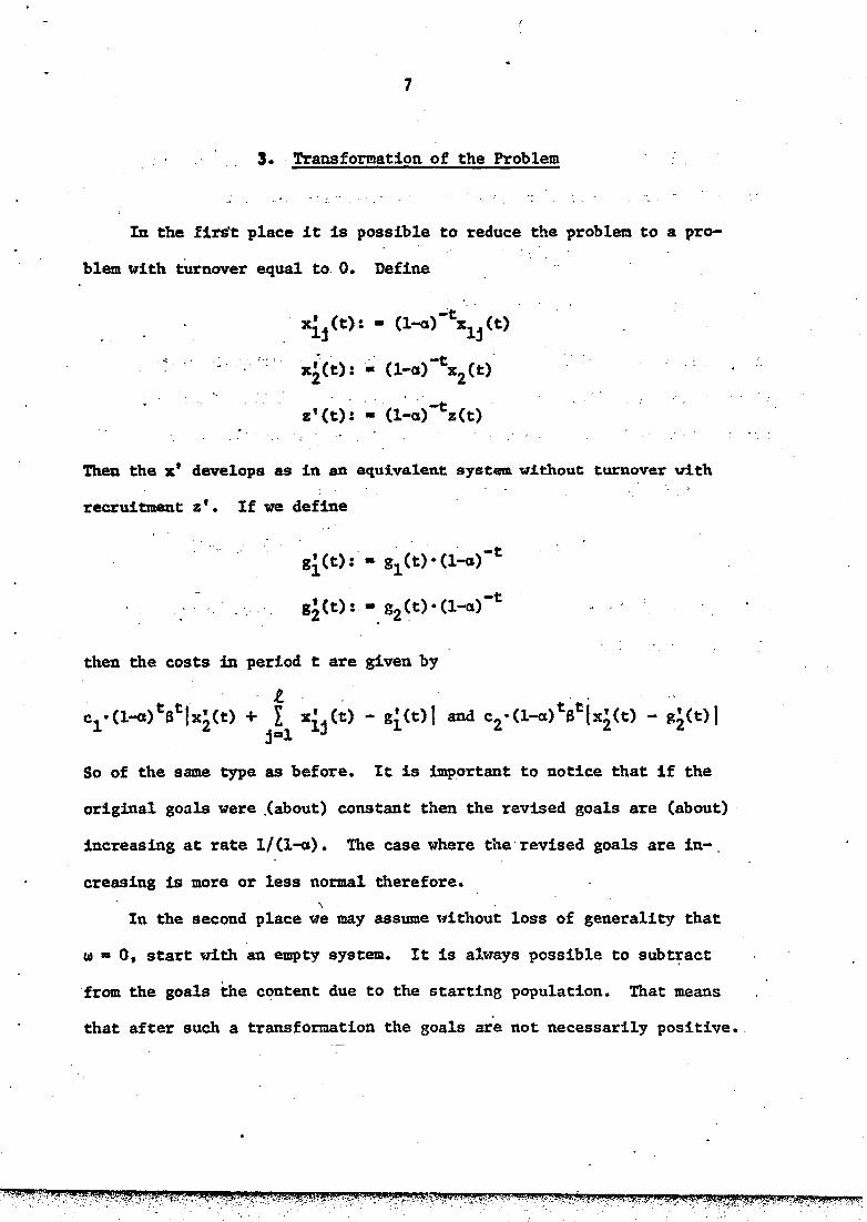
3. Transformation of the Problem

. '·:

In the lirst place it is possible to reduce the problem to a pro­

blem with turnover equal to O. Define

·•

..

xij(t): • (1-a)~txlj(t) ; .. ' ·. . -t .

x2Ct): • (1-a) x2(t)

-t . z'(t): • (1-a) z(t)

Then the x' develops as in an equivalent system w~thout turnover vi.th

recruitment z'. If we define

then the costs in period t are given by

So of the same type as before. It is important to notice that if the

original goals were _(about) constant then the revised goals are (about) ·

increasing at rate 1/(1-a). The case where the revised goals are in-

creasing is more or less normal therefore.

" In the second place we may assume ''ithout loss of generality that

w • 0, start with an empty system •. It is always possible to subt~act

from the goals the content due to the starting population. That means

that after such a transformation the goals are not necessarily positive.

8

The third transformation is the most important one. It reduces

the problem to an equivalent problem without grade-age. Let

t -· y.1Ct): • I xijCt) + x2(t)

j•l

y2(t): • :X:i(t)._

All people in the system at time t are.at time t+t-1· either in state . 4

(1,l) or in state (2). So xU.Ct+t-1) • y1(t) - y2Ct+l-l). The hput

at time t+l from _grade 1 to grade 2 is p(y1(t) - y2Ct+l-l)). Hence

Y2Ct+t) - Y2Ct+l-l) + p(yl(t) - Y2Ct+l-l))

. t-1 i . - (l-p)y2(t+l-l) +.PY1(t) • p I (1-p) yl(t-1)

· . i•O

Y2(t+l) Now define y; ( t) : • P , then the problem is to choose y 1 ( •) such

that the expression

is ~nimized under the conditions Yi (1) ~ O, y1 (t+l) ~ y1 (t), t • 1,2, •••

(since the total content at time t+l can never be less than the total

content at timG t). 'The relationship between y1 and v; is given by

t~ i . . . y~(t) • I (l-p) Y1 <.~-i) • Y1 (t) + (l-p)y~(t-1)

i=O

So we may view y1(·) and y;(•) as input and content of a system where

each period a fraction p of the old population leaves (see Figure ~2) •

:;f§'i¥WWWfftMW-·'tr·mtrmmzrwwrnmennrewwmmzwx··r rr-xwwwwwrn·wrrrre11 :rr

9

--1--content is y 2 ( •)

Pigure 2

For cases with more grades one can get the same tyP.e of transfor-·

mation. If there are k grades in the original system tdth ~, ••• ·~-l

the maximal grade-ages and p1, ••• ,pk-l the promotion probabilities

from the highest grade-age to the next grade, then the system is

equivalent to a system as depicted in Figure 3 • The total content

in the original system corresponds to the input in the transformed

system, the total content of the grades 2, ••• ,k in the original system

corresponds to the content of state 1 in the transformed system, and

so on.

y. ( ·) k •

Figure 3

y1

( •) (input)

10

.~; ·. . 4. The One-Level Case

-.

In this section we consider the case in which there is a single

grade. According to Section 3 the problem is then to

T . Minimize I {djy(t) - h(t)f (1-a)tBt}

t•l

under the conditions y(l) .?. 0 and y(t+l) ~ y(t) for t .?. 1. Since the

goals h(•) are tl:ansformed to take into account the contribution due

to the starting content, it is possible that h(t) < O. The one-level

case is interesting in its own right, but also bea:xiae of its similarity

with the two-level case with promotion probability p • 1 (see Subsec-

tion 5.1).

In the single-level case it is possible to give an explicit expres- ·

sion for the optimal first-period decision. This can be ~ed to derive

planning horizon results •. Let y(tf T) be the optimal content in period

t for the T-period problem. Define sgut(x): = -1 for x ~ h(t), - tl t t

sgut(x): = +1 for x > h(t).t Let st (x):. I {sgut(x)(l-ci) a} and . - 1 t•l

let ~ be the supremum of all x sucl1 that st1

(x) ~ 0 for all t1 ~ T. _

Notice that D.r~h(l}.

An integer T* is called a planning horiz~n if y(llT> = y(l!T*)

for all T.?. T*, independent of the h(t) for t > T*. T* is called a • J.4'. ,' < • ' ;~_.

(weak) planning horizon if y(l!T) • y(l(T*) is only true under certain

conditions on the h(t) for t > T*.

Lemta 4.1. y(llT) = max(O, nT) for all T ~ 1~

11

Proof~ Suppose y(l(T) > max(O, nT) for some T. Let t1 be the first

.t1 such that st (y(l!T)) > O. Construct the solution y'(•) by 1

y'(t) • y(tjT) - & for all t.!_ t1 and y'(t) • y(tfT) ·for all t > t1•

Then, by the definition of st , the solution y'(•) is better than the 1

solution y( ·IT), which yields a contradiction.

s.uppos~ now that y(llT> < ~(O, n.r>, ~o o !. y(llT> < ~· Let t'

be the first t such that y(t IT) ~ max(O, ~) (if. such a t exists; other­

wise t': • T + 1). Construct. the solution y'(•) by y'(t) • max(O, ti.r> for t < t* and y'(t) • y(tfT) for t .! t'. By the definition of °'r the

solution y.' ( •) is cheaper than the solution y ( • IT) , whiu yields a

contradiction again. · ·

The following corollaries are immediate consequences of Lemma 4.1.

Corollary 4.1. The optimal first-period decision y(lf T) is non- ·

increasing in T. That means,. if y(lf T*) • 0 then T* is a planning

horizon.

Corollary 4.2. If .h(t) ~h(l) for all t > t then t is a (weak) plan-. - 0 O·

ning horizon.

A special case where the conditions of Corollary 4.2 are satisfied

for t • 1 is the case where h(t) is increasing. The optimal policy is 0 .

myopic in this case, y(l!T) • max(O, h(l)). In sect~on 3 w~ mentioned

already that the case of increasing (revised) goals is the normal case.

The discount ~actor $ and the turnover rate a can also help in

getting planning horizons.

12

* * -(l-a)t +18t +l Corollary 4.3. If for t* .!, 1 the value st*(h(l)) ..::. 1-(l-a)B

then t* is a planning horizon.

Proof.

all t .!. t*. Since~..::. h(l) this implies that~ is constant for

T .!, t*.

For instance, if (t-a)B s i then s1 (h(l)) = - (1-a)B

'. 2 2 -(1-a) B

s 1-(1-a)B

= - (1-a) 2B2 (1-a)B s

and corollary 4.3 implies that 1 is a planning horizon, ~ = h(l)

13 '

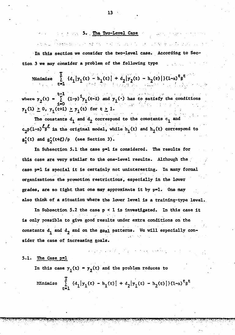
- ' ,·, ·; s •.. The. Two-Level Case , .. ·

··- .' ·"': ~ ~ .. : ; '.. ... :: .· '' . !• ' ·'

·In this section we consider the two-level case. According to Sec-

tion 3 we may consider a problem of the following type

Minimize

t-1 ~here y2 (t) •· l

i•O (l-p) 1y

1C.t-·i) and:y

1C:) hast~ ~~~fsfy the co~ditions

. . .

Yi(~) .?. O, yl (t+l) ,?. y1 (t) for t > 1. -I. /' .,, •. ••

The constants d1 and ·d2 correspond to the constants c1 and . . , I.. t . . . . . . .

c2p(l-a) B in the original model, while h1(t) and h2(t) correspond to

gi(t) and gi(t+l..)/p (see Section 3).

In Subsection S.l the c;ase p•l is considered. The results for

this case are very similar to the one-level results. Although the :

case p•l is special it is certainly not uninteresting. In many formal

organizations the pr~otion restrictions, especially in the lower

grades, are so tight that one may .approximate it by pl!lll. One may

also think of a situation where the lower level is a training-type level, •.

In Subsection 5.2 the case p < 1 is investigated. In this case it . ·.

is only possible to give good results under extra conditions on the I

constants d1 and d2 and on the goal patterns. We will especially con-.. .: . .'

sider the case of increasing goals.

5.1. The Case p•l

In this case y1(t) • y2(t) and the probl~ reduces to

T ?il.nimize l {d1 jy1(t) - h1(t)( + d2 1y~(t) - h2(t)f }(1-a)tBt .·

t=l

14

uuder the conditions y1(1) _! 0 and y1(t+l).?. y1(t} fort.?. 1. That

. means that this problem is almost equivalent to the one-level case.

i.JJ·ill that case there is only one variable which can be controlled.

The difference is the shape of the·penalty function.

Let ;ic0(t) be the largest v~lue ~£ x for which d1 1x - h1 Ct>.1 +

d21x - h2(t)f ~·minimal. ~~ ~~(x} .be .the left-hand d~ri~ative of

th~ function in x. D~fin~. as fn Section 4, for all t 1 .?. l~ . . . . tl . . t t . . .·. . . . . ' . ·. st (x) : • I rt (x) (1-ci) 8 ~ let ~ be the supremum of all x such

1 t•l .. that st

1 (x) ~ 0 :for. ~ t 1 ~ T. -~bserve that nt ~ x0 (1). The. foll~

ing lemma ·and corollaries correspond to Lemma 4.1 and.Corollaries 4.1. . .

4.2 and 4.3, and are given without proof.

Lemma 5.i. For each T there in an optimal solution y1 Ct IT) ~tith

y1

CllT) • max(O, f1.r)• ....

. .

Corollary 5.1~ If y1CllT*) • 0 then·T* is a planning horizon.

Corollary s.2. If h_(t) and h2(t) are such that ·x (t) > x (1) for. --i 0 - 0

all t > t then t is a (weak) planning horizon. - 0 . 0

t, ..

A special case where these conditions are satisfied for t • 1 is 0

the cas~ ~ere ~1(•) and ~2(•) are increasin~; this implies that x0(•)

is also increasing. In this case Y1 CllT> - max(O, xoc1)1. -

Corollary S.3. If for certain t* .?. l the value

> .r then t* is a planning horizon. ·

·;~':f~f:.1~tt'Y'ffij;;,-;.z¥tt&#ZltHfiiWG*i'''ift'M f"WK"'··rtn rm WttntfM1 trr··m·-;n=:rf'·nrz=,.: T2

Zt=vwnr~·n zsn55FS'7T~- a1mram~WMrmr·rsr ·w· ·

/

--15

·· ·since the transformations applied in Section 3 are more essential

in this case than.in the one-level case we have to check what a planning

horizon T in this transformed model means in the original problem. The

main part of the transformation was a shift in the time-axis for y • . 2

That means that a planning horizon T for the transformed problem implies

that in the origin.al P,roblem _o!3e .!leeds t~ .Jcnc:ni the_ goals g1

(1), ••• ,~ (T) ~~;£,; ... :: .,; ..... ·. - ..... 't· ··--····--·

and g2(1), ••• ,~2 ~T-f-:)_.In case p=l the maximum time sperit in the lowest - -

grade is £. The result shows that £ contributes directly to the length of

the proper planning horizon.

Reviewing this subsectio~ shows that the results can be generalized

to the case with more than two levels and more general penalty functions.

5.1. The Case p < 1

In this case one has to add conditions on the ratio of d1 and d2•

If d1/d2 is large and h1(•) can be followed (h1(•) is non-decreasing)

then h1(·) has ~o be followed indeed. If d2/d1 is large and h2(•) can

be followed then h2(·) has to be followed indeed. However, there is a ·-

gap between the two regions; a gap which is widening with decreasing p.

In Lemma 5.2 we consider the case where !11 is the most important goal. ·

Lemma 5.2. Let d1 > d2/p and h1(t) non-decreasing for

for each T the optimal solution y1CtlT> satisfies

t > t • - 0

for all t > t • - ·O

Then

Proof. We tiill give the proof for the case a = O, B • l; the proof

for the general case is similar.

Let t 1 ~ t 0 and suppose y1Ct1 jT) > max(h1Ct1), y1Ct1-1IT)). Then

the optimal solutio~.c.an be... improved by the revised solution yi(•) .

16

defined by yi(t) • y1CtJT), t ~ t 1 and Yi<t1) • y1Ct11T) .- e:.· ·The total

cost for deviations from goal h1(·) is e:d1 less for solution Yi(•) than

for y1

C·fT), while the cost for deviations from goal h2(•) is at most . 2 ~2

e:(d2

+ d2(1-p) + d2 Ct~p) + ••• ) • p .. more for Yi(•) than for -..· ~

y1

( • JT). · Tllis yields a contradiction.·· .· . . .. ~

NoW suppose y1Ct1fT) < h1Ct1) for some t 1 !. t0

• Let t 1 + k be the

first period t where y1CtfT) !. h1Ct) (if such a· period exists; otherwise

t 1+ k: • T + 1). This implies that y1Ct1+kfT) > y1Ct1+k-lfT). Define

YiCt1+k): • y1Ct1+k!T) - e(l-p)k

. Yi(t): • y1CtJT), t ~ t 1, t 1 + k ·

This is pos~ible fore: small eno~gh. since y1(t1+k!T) > y1Ct1+k~l(T). Now Yi(•) differs from y2C·IT> only in the periods t 1, ••• ,t1+k-1. The

reduction in costs of deviations from the goal h1(·) is .at least k . .·

(d1 - (1-p) d1)e while the increase in costs of deviations from the

k-1 k goal h2(•) is at most e(d2 + d2Cl-p) + ••• + d2(l-p) ) • e•d2/p(l - (1-p) ).

So in total y'(•) is better than yC•IT), Yhich yields a contradiction.

In case h1(•) is increasins the conditions of Lemma 5.2 are

satisfied for t • l. We have the follauing corollary. 0

Corollary 5.4. If d1 > d2/p and h1C·) is increasing then the optimal

first-period decision is y1 Cl!T> • ma.~{O, ~1 (1)) and l is therefore a

(l1eak) planning horizon ..

17

For t > 1 the problem is more difficult here than in the one-level 0

case or the two-level.case with p•l. tn the first part of the proof we

do not use the ~act that h1(·) is non-decreasing. That means that

y1

(tjT)S max(h1(t); y1(t-ljT)) for all t. Lett*~ t0

be such that

. h1 (t*) ~ h1 (s) for all s < t0

and also· hl. (t*)- ~ O. Then for all problems

with T ~ t* the optimal y 1 (t*lT) = h1

Ct*) • . '

However, this does not necessarily mean that

t* is a planning horizon, since y2(t*) is still free and 1d.ll depend in

general on the behavior of h2(·) and h1(·) beyond t*.

In the next lemma we consider the case 1Jhere h2 ( •) is the most

important go'il.

Lemma 5.3. Let d2 > d1(2-p) and let h2Ct+l) - (1-p)h2(t) be non­

decreasins. from t = t0

- 1 on. ~en f11Jr each T the optimal solution

y1C·IT), 12C·IT) has the following properties.

(a) k k Let t 1 ,?. t0

and let y1C•),_y2(•) be a feasible so~ution such that

y~(t) •y1 (tj"tl for t s t 1 - 1, y~(t) s li2(tf for t .~ ~l and k . . k .

y2Ct) • h2(t) for t !. t 1 + k. Then y2(t11T> !. y2Ct1).

(b) If (l-p)y2Ct1-ljT} + y1 Ct1-llT> .!, h 2Ct1

) for some t1

.?. t0

then

Y2<t1IT> .!_h2Ct1>·

(c) If (1-p)y2Ct1-ljT) + y1 Ct1-llT> !, h2Ct1) for some t1

!. t0

then

Y1<t1fT) - Y1<t1-l(T).

Proof. We will give the proof for the case where ~ • O, B • l; the

proof for the general case is similar.

mar itriFM

.•

18

k . k 1~ .. (a) ·Let y

1(·)t y

2(·) be as stated. Suppose·y2(t1 1T) < y2Ct1). ···Choose

t such that t1

+ t is the first period t after t 1 such that .i

11

CtJT) »Yi Ct-llT) (if such a period exists; otherirlse t1+t:-· • T+l).

Then y 2

( t IT)·-< y~( t) for ti .! t < t 1 · + l.. ·Define the revised solu- :

. ·.:. . .. ~

. . ·:· --: ..... ~ ~ f' ., : v • ••••• •

· .... •\

•. -~· J · ..

' :~ . . . ... . . .. .;·. ·.:" .

YiCt1+~~: • y1Ct1fT) .i+- £, ~ • O~l, •• ~,t~l . -· . . . ... ; . -~ ~ ·~ ....

; • ~ •. "" ••• ,·"4

t .. Yi (t1+t): • Y1 C~1+tj T),. - e{ (1-p) + (1-P.>.

2 + •. ~ .+ (1-p) .1_ ..

~ yi(t): • y1

CtJT),- t < t 1 and t > t1

+ t. : · · .: .

Si~~e y~(t» ~,~2~tl for .t ~ t~ a~d y2 (t·I~;· < y~(~). fo~· t1

.i_ t <, t1

+ l., 'k

we have also yi(t) < y2(t) .! h2(t) for t 1 ~ t < t 1 + I.. (and £

sufficiently· small) • · For t ~ t 1 + I.. ~fe have y 2 ( t) • y 2 ( t IT) •

The reduction in cost of deviations from the goal h 2(·) is equal· t-1 t-1 1+1 .

to d2 I ec1 + c1-p> + ••• + c1-p>1> • d2e r 1-<1-p> • i=O i=O P

. d. ,,.c&. - 1-e· i-c1-p>t:\ ·•· . . . .- .. 2

.. p p p ., · The. increase in cost of deviations from . . . . :. · . . : . . - . .. t'" . ' .

the goal .h1

(• >. is at most dite· + d1-rtt-p) l-(~-p) • •It. is• e~~?' ...

to prove by induction, using d2 > d1(2-p), that the total cost of .., .

y i C-·) ~ y 2 ( •) is less than th_e to:al cost of y 1 ( • IT) , y 2 ( • IT) , · ·

which contradicts the optimality of this last solution.

(b) Let (l-p)y2

Ct1-ljT) + y

1 (~1-l!T) .! h 2Ct

1) for some· t

1'.?.. t

0 and ·'

suppose y2

Ct1

fT) > h2

Ct1). Observe first that by part a and:the

non-decreasingne~s of h2 ~t+l) - (l-p)h2(t) from t = t0

- 1 on this . . -'•• .

implies that y 2CtjT) ~ h2(t) fo~ .·all ~ ~ t 1 • Choose l such that .. "

19

t 1+t is the first peri.od t after t 1 such that y2CtlT> • h2(t) (if

such a period exists; otherwise t 1+t: • T+l). Define the revised

solution Yi(•), Yi(•) by. ... :

YiCt1): • y1 Ct1 fT) - c . . , ·-.

YiCt1+t): • y1Ct1+tfT) _+ c(l-p)t

Yi (t}: • y1 (tf T) for all t rf. t 1, t 1 ·+ l..

. The _feasibility of Yi Ct1): • y1 Ct1 f T) - e follcn1s .from

(l-p)y2Ct1-l[T) + y1Ct1-lfT) ~ h2Ct1) and y2Ct11T> • (l-p)y2Ct1-llT> +

y1Ct1 fT) > h2Ct1), which implies that y1Ct1 fT) > y1(t1-l(T} and

therefore that y1Ct11T) can be reduced indeed. That y1Ct1+t!T)

. can be increased wi.thout increasing y 1 ( t IT) for t > t1 +t, follows

from y1 Ct1+t+llT> ~ h2 Ct1+t-t-:l) - (1-p)h2Ct1+t) • h 2Ct1+t+l) -

_(l-p~y2 Ct1+t) !. h2Ct1+t) - (l-p)h2Ct1+t-l) > y2(t1+tf T) -

12 Ct1+t-1IT>_~ y1Ct1+lfT) •

. For yi(•) !~have .. • .

"<'

Yi(t) • y2Ct!T), t < t 1

Yi(t+i) • y2(t+ifT) - c(l-p)1, i = 0,1, ••• ,t~l

. Yi(t) = 12CtlT), t !. t 1 + t

The reduction in cost of deviations from the goal h2(•) is

t-1 . t . d

2e L (l.;..p) 1 • d

2e l-(;-'D) • .The increase in cost of deviations ·

i=O . . t from the ~oal h1 (·) is at most d1e + d1e(l-p) • From d2 > d

1(2-p)

it follows that the total cost of Yi(•), yi(·) is less than the

/

20

·- ----- ... ·--·-·- ·-----

total cost of y1

(•(T), y2C•(T), which contradicts the optimality

of the last solution.

(c) The proof of c is similar to the proof of b.

Application of this lemma to the case ,;fith to·= 1 (with h2(0): • 0)

gives also myopic-type _results. In the first. place, it follol'1S from c

·that h2

(1) ~ 0 implies y1

(l(T) • o: So in this case the (weak) planning

horizon is indeed equal to 1. Further, it follows from a and b that if

there is a feasible policy y~(·)~ y2(·) y~th y~(t) = h2Gt) for all t ~ 1

·then this ls t~~ optimal pol~c~-. Sin~e h2{2) - (l-~-;=~~~(1) ;:;~h~c'1{:-~-" ·

such a policy yl(-), y~(-) exists if h2(1) ~ 0. So.i.n this case the

. (weak) planning horizon is equal to 2 (and y1CllT) = h2(1)).

To.evaluate the usefulness of Lemm.a S.3.observe that

h2(t+l) - (l-p)h2_(t) <:: h2(t) - (l-p)h2(t-l) can also be written

h2(t+l) - h2(t) <:: (l-p)(h2(t) - h2(t-l)). So convexity of h2(•) is

sufficient for all p, but for the case where p is close to 1 the con-

dition is much weaker. According to section 3 one may expect in most

cases h2(·) increasing about geometrically. That means that the condition

is not too severe. '< ...

. 21

- .

6 •. Production-Smoothing Problem

In this section ,,e discuss the relationship of this problem with

the production-smoothing problem without inventory investigated by

Aronson. Morton. Thompson (1). First we apply one more transformation.

Define y 1 ( t) : . - y 1 ( t) - bl ( t) . . .. '. .. . t-1 .

Y2(t): • Y2(t) - I (l-p)1ii1<t-i) .. · . i•O .

The problem formulated in y1 and y2 is then

.T t-1 llinimize I {d1IY1Ct>I + d2fy2(t) - (h2(t) - I (l-p)~l(t-i)(}(l-a)t8t

t•l .. • . . . i•O · .. .. .·:

. t-1 where 12Ct) • L (l-p)iy1(t-i) and y1(·) has to satisfy the conditions

i-0 .

for t > 1.

The problem ·considered in [l] is of the following type

T }li.Dimize I {alx1(t)( + bfx2(t) - d(t)ll

t==l

. t-1 where x2(t) • I x1Ct-i).

i•O

'·:

-

The most essential difference is that in the problem considered

here y1(•) is not free while in the production-smoothing problem ~1 (•) is free. In [1] the following planning horizon result is given. If

for certain T • T* the optimal policy is such that x1(t1) > 0 atid

x1Ct2) < 0 for certain t 1 ~ t 2 smaller than T* then the optimal policy

on the interval [1, min(t1, t 2) - l] is not chaneed by a further

increase of T.

•

• 22

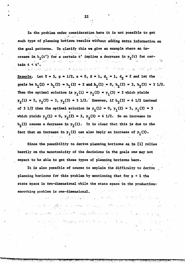
In the problem under consideration here it is not possible to get .;... # •• ••

such type of planning ho~izon resuit~ without adding i1'Xtra inf otmation on

the goal patterns. To clarify this we give an example where an in­

creas~; in h2Ct') for a certa~-- t' htPlies' a. ~e.crease in y2(t) for cer-... ". ' . .·. ··:.·

tain t <. t'. • . 4, . • • .• ~-· •• · .. , . : ' . ·~ ~ :... . .

Examrle. Let T • 3, p • 1/2, a·-~' $ • 1. dl • 1, ~2 • 2 and let the

goals be hl(l). ~(2) •_hl(3). 2 ~4.h2(1) .• o,_h2(2). 3, h2(3). 3 1/2.

Then the optimal solution is y1(1) • y1(2) • y1(3) • 2 "fhicb yields

.y2Cl) • 2, Y2(2) • 3, y2(3) • 3 1/2. How~er, if h2(3) • 4 1/2 instead

of 3 1/2 then the ~~imal soluti:on is y1(1) • 0, y1(2) • 3, y1(3) • 3 . . . . .

which yields y2(1) • O, y2(2) • 3, y2(3) • 4 1/2. So an increase in

~ (3) causes a decrea~e in y 2 (1). It is clear that this is due to the

fact that an: increase in y1(2) can also imply an increase of y1(3).

Since the possibility to derive planning horizons a~ in [l] relies

heavily on the monotonicity of the decisions in the goals one may not

expect to be able to get these types of planning horizons here.

It is also possible of course to explain the difficulty to derive

planning horizons for this problem by mentioning that for p < 1 the

state space is two..:dimensiona.l.while the state space in the production-

smoothing problem ~s one-dimensional •

........ • • 1 ..

. , .

;~ ..

• •

•

_[1]

23

References

" . Aronson, J.~., Morton, T.E., Thompson, G.E. (1978), A Forward Algorithm and Planning Horizon Procedure for the·Production­Smoothing Problem Without Inventory", Carnegie-Mellon, Report W.P. 20-78-79.

- ---·--- -- - -- - --- -·-----~ ----- __ .;...... ________________ _ [2] Baker, K.R., Peterson, D.W. (1979) "An Analytic Framework' for

0 __

.Ev.aluating Rolling Schedules", -Management Science, 25, 341~~51. -------·- ··--"'--·"'-·~-- - -- - - - ---·---- -· . --- -- -·- -- ·-- - ·--- - .... --- . - -

[3}

{4]

[5]

... - -------------- ---van der Beek,. E., Verhoeven, c. J. , Wessels, J. (1977) , "Some Applications of the Manpower Planning System FOR!.fASY", llanp. Pl. Rep., No. 6, Eindhoven University of Techn~logy.

Charnes, A., Cooper, W.W., Ler.ds, K.A., Niehaus, R.J. (1978), "Equal Employment Opportunity Planning and Staffing Models", pp. 367-382 in D. Bryant and R.H. Niehaus (Eds.) !fanpm1er Planning and Organization Design. Plenum Publishing Corp., New York.

Lundin, R., Morton, T.E. (1975), "Planning Horizons for the Dyna­mic Lot Size rtodel: Zabel vs. Protective Procedures and Computa­tional P..esultstt, Oper. Res., 23, 711-734.

[6] Morton, T.E. (1978), "Universal Planning Horizons for Generalized Convex Production Scheduling", Oper. Res., l§., 1046-1058.