planning for cooperative persistent long term autonomous...
TRANSCRIPT
UNIVERSIDADE ESTADUAL DE CAMPINASFACULDADE DE ENGENHARIA MECANICA
Rodolfo Jordao
Planning for Cooperative Persistent LongTerm Autonomous Missions
Planejamento para Missoes AutonomasPersistentes Cooperativas de Longo Prazo
CAMPINAS2018
Rodolfo Jordao
Planning for Cooperative Persistent LongTerm Autonomous Missions
Planejamento para Missoes AutonomasPersistentes Cooperativas de Longo Prazo
Master’s thesis presented to the School of Mechan-ical Engineering of the University of Campinas, asone of the requirements for the Mechanical Engi-neering Masters program, in the area of Solid Me-chanics and Mechanical Design.
Dissertacao de Mestrado apresentada a Faculdadede Engenharia Mecanica da Universidade Estad-ual de Campinas como parte dos requisitos exigidospara obtencao do tıtulo de Mestre em EngenhariaMecanica, na Area de Mecanica dos Solidos e Pro-jeto Mecanico.
Advisor: Prof. Dr. Andre Ricardo Fioravanti
ESTE EXEMPLAR CORRESPONDE A VERSAO FI-NAL DA DISSERTACAO DEFENDIDA PELO ALUNORODOLFO JORDAO, E ORIENTADO PELO PROF. DR.ANDRE RICARDO FIORAVANTI.
ASSINATURA DO ORIENTADOR
CAMPINAS2018

Agência(s) de fomento e nº(s) de processo(s): CAPES, 1687532ORCID: https://orcid.org/0000-0002-1277-390
Ficha catalográficaUniversidade Estadual de Campinas
Biblioteca da Área de Engenharia e ArquiteturaLuciana Pietrosanto Milla - CRB 8/8129
Jordão, Rodolfo, 1993- J767p JorPlanning for cooperative persistent long term autonomous missions /
Rodolfo Jordão. – Campinas, SP : [s.n.], 2018.
JorOrientador: Andre Ricardo Fioravanti. JorDissertação (mestrado) – Universidade Estadual de Campinas, Faculdade
de Engenharia Mecânica.
Jor1. Planejamento. 2. Robótica. I. Fioravanti, Andre Ricardo, 1982-. II.
Universidade Estadual de Campinas. Faculdade de Engenharia Mecânica. III.Título.
Informações para Biblioteca Digital
Título em outro idioma: Planejamento para missões autônomas persistentes cooperativasde longo prazoPalavras-chave em inglês:PlanningRoboticsÁrea de concentração: Mecânica dos Sólidos e Projeto MecânicoTitulação: Mestre em Engenharia MecânicaBanca examinadora:Andre Ricardo Fioravanti [Orientador]Leonardo Tomazeli DuarteRomis Ribeiro de Faissol AttuxData de defesa: 26-02-2018Programa de Pós-Graduação: Engenharia Mecânica
Powered by TCPDF (www.tcpdf.org)

UNIVERSIDADE ESTADUAL DE CAMPINAS
FACULDADE DE ENGENHARIA MECANICA
COMISSAO DE POS-GRADUACAO EM ENGENHARIA MECANICA
DEPARTAMENTO DE MECANICA COMPUTACIONAL
DISSERTACAO DE MESTRADO ACADEMICO
Planning for Cooperative Persistent LongTerm Autonomous Missions
Planejamento para Missoes AutonomasPersistentes Cooperativas de Longo Prazo
Autor: Rodolfo JordaoOrientador: Prof. Dr. Andre Ricardo Fioravanti
A banca examinadora composta pelos membros abaixo aprovou esta tese:
Prof. Dr. Andre Ricardo FioravantiFaculdade de Engenharia Mecanica
Prof. Dr. Romis Ribeiro de Faissol AttuxFaculdade de Engenharia Eletrica e de Computacao
Prof. Dr. Leonardo Tomazeli DuarteFaculdade de Ciencias Aplicadas
A Ata da defesa com as respectivas assinaturas dos membros encontra-se no processo de vida academicado aluno.
Campinas, 26 de Feveiro de 2018

Acknowledgements
I’m very grateful to my advisors, parents, friends and close ones for their continuous support, and alsoto CAPES for financing my studies, which this works would not have existed otherwise.

Resumo
Uma metodologia para abordar missoes autonomas persistentes a longo prazo e apresentada junta-mente com uma formalizacao geral do problema em hipoteses simples. E derivada uma realizacao dessametodologia que reduz o problema geral para subproblemas de construcao de caminho e de otimizacaocombinatoria, que sao tratados com heurısticas para a computacao de solucao viavel. Quatro estudos decaso sao propostos e resolvidos com esta metodologia, mostrando que e possıvel obter caminhos contınuosotimos ou subotimos aceitaveis a partir de uma representacao discreta e elucidando algumas propriedadesde solucao nesses diferentes cenarios, construindo bases para futuras escolhas educadas entre o uso demetodos exatos ou heurısticos.
Palavras-chave: Planejamento, Roteamento, Design de Metodologia, Robotica Cooperativa

Abstract
A Methodology for tackling Persistent Long Term Autonomous Missions is presented along witha general formalization of the problem upon simple assumptions. A realization of this methodologyis derived which reduces the overall problem to a path construction and a combinatorial optimizationsubproblems, which are treated themselves with heuristics for feasible solution computation. Four casestudies are proposed and solved with this methodology, showing that it is possible to obtain optimal oracceptable suboptimal continuous paths from a discrete representation, and elucidating some solutionproperties in these different scenarios, building bases for future educated choices between use of exactmethods over heuristics.
Keywords: Planning, Routing, Methodology Design, Cooperative Robotics

List of Figures
1.1 Example of a Persistent Long Term Mission with sampling and surveillance objectives. . 131.2 Deforestation of Brazil’s Amazon legal region, from 1988 to 2016. . . . . . . . . . . . . . . 141.3 Airship Projects . . . . . . . . . . . . . . . . . . . . . . . . . . . . . . . . . . . . . . . . . 141.4 Overall autonomous platform view and its inter-relations. . . . . . . . . . . . . . . . . . . 16
2.1 Mission planning workflow diagram. . . . . . . . . . . . . . . . . . . . . . . . . . . . . . . 182.2 Two examples to highlight the segmentation effect on the drift from the best true path
obtained after segmentation. . . . . . . . . . . . . . . . . . . . . . . . . . . . . . . . . . . . 192.3 Two examples of reconstruction after position planning (left) and during position planning
(right) highlighting the necessity of treating orientation with positioning. . . . . . . . . . 192.4 Visual representation of the lattice used in the segmentation. In this case showing the
maximum possible lattice gap. . . . . . . . . . . . . . . . . . . . . . . . . . . . . . . . . . 202.5 Example of primitive and neighborhood definitions. . . . . . . . . . . . . . . . . . . . . . . 202.6 Constituent simpler elements of a complex maneuver. . . . . . . . . . . . . . . . . . . . . 202.7 Example of equivalent lattices achieved via displacement. The left lattice is the original,
the middle lattice is the same as the left one, but displaced diagonally, and the right one isthe lattice obtained by displacing a full diagonal from the left one and half diagonal fromthe middle one. . . . . . . . . . . . . . . . . . . . . . . . . . . . . . . . . . . . . . . . . . . 21
2.8 Intervals of search for positioning. . . . . . . . . . . . . . . . . . . . . . . . . . . . . . . . 222.9 Two different continuous reconstruction with cohesive node links. . . . . . . . . . . . . . . 262.10 Example of possible problems with relaxed model limits. . . . . . . . . . . . . . . . . . . . 282.11 Illustration of the tour merge transformation. . . . . . . . . . . . . . . . . . . . . . . . . . 302.12 Illustration of the tour removal transformation. . . . . . . . . . . . . . . . . . . . . . . . . 302.13 Illustration of the node transfer transformation. . . . . . . . . . . . . . . . . . . . . . . . . 302.14 Illustration of the node removal transformation. . . . . . . . . . . . . . . . . . . . . . . . . 312.15 Ray casting algorithm visualization. . . . . . . . . . . . . . . . . . . . . . . . . . . . . . . 342.16 Simple convex region and its segmentation objective function. . . . . . . . . . . . . . . . . 352.17 Result of filtering for interest nodes after segmentation. . . . . . . . . . . . . . . . . . . . 35
3.1 Point cloud and cell graph of case 1. . . . . . . . . . . . . . . . . . . . . . . . . . . . . . . 393.2 Filtered interest nodes for case 1 with their covering radii. . . . . . . . . . . . . . . . . . . 403.3 Sample of all constructed paths for case 1. . . . . . . . . . . . . . . . . . . . . . . . . . . . 413.4 Resulting tours for exact and ASC solutions of case 1. . . . . . . . . . . . . . . . . . . . . 423.5 Resulting tours for exact and ASC solutions of case 2. . . . . . . . . . . . . . . . . . . . . 433.6 Resulting tours for a ASC+OOS solution of case 3. . . . . . . . . . . . . . . . . . . . . . . 443.7 Resulting tours for exact solution of case 3. . . . . . . . . . . . . . . . . . . . . . . . . . . 453.8 Resulting tours for a ASC+OOS solution of case 4. . . . . . . . . . . . . . . . . . . . . . . 463.9 Resulting tours for exact solution of case 4. . . . . . . . . . . . . . . . . . . . . . . . . . . 47

List of Algorithms
1 Eager Uniform Cost Search (Dijkstra’s algorithm) . . . . . . . . . . . . . . . . . . . . . . 252 Lazy Uniform Cost Search . . . . . . . . . . . . . . . . . . . . . . . . . . . . . . . . . . . . 253 ASC . . . . . . . . . . . . . . . . . . . . . . . . . . . . . . . . . . . . . . . . . . . . . . . . 294 OOS . . . . . . . . . . . . . . . . . . . . . . . . . . . . . . . . . . . . . . . . . . . . . . . . 325 ReSC . . . . . . . . . . . . . . . . . . . . . . . . . . . . . . . . . . . . . . . . . . . . . . . 336 Polygon pertinence ray casting algorithm . . . . . . . . . . . . . . . . . . . . . . . . . . . 35

Glossary
ASC Admissible Score Clustering. 39, 42, 44, 45, 49, 50, 60, 63
AURORA Autonomous Unmanned Remote Monitoring Robotic Airship. 24
CTI Centro de Tecnologia de Informacao Renator Archer.
CVRP Capacited Vehicle Routing Problem.
DRONI Conceptually Innovative Robotic Airship. 24
MILP Mixed Integer Linear Programming. 35, 37, 39, 42, 63
OOS Order and Orientation Switching. 42, 44, 49, 50, 60
PLTAM Persistent Long Term Autonomous Mission. 23–26, 29, 35
ReSC Restarting Sequential Construction. 42, 49, 50, 60
ShorPaP Shortest Path Problem. 30, 35, 36, 63
SimPaD Simple Path Drift. 30, 32, 63
TSP Traveling Salesman Problem. 39, 42
UAV Unmanned Air Vehicle. 25, 49, 50
UGV Unmanned Ground Vehicle. 34, 49, 50
VRP Vehicle Routing Problem. 29, 30, 39
Symbols
Ec+ Cell graph edges, being primitives.
Ed+ Decision graph edges, being primitives.
Gc Cell graph, resulting from segmentation.
Gd Decision graph, resulting from path construction.
Ia Index of agent classes.
Io Index of operations.
Ir Index of interest regions.
N c+ Cell graph nodes, being positions and orientations.
Nd+ Decision graph nodes, being positions and orientations.
Ri Sub interest region of index i.
R Working total region.
βa Capacity limits for agent class a.
N Set containing all natural numbers (without zero).
R Set containing all real numbers.
P(bR) Set of discrete paths that originate and end in bR.
PC(bR) Set of discrete paths that originate and end in any other point than bR.
S(bR) Set of continous paths that originate and end in bR.
S(p1, p2) Set of continous paths that originate in p1 and end in p2.
T Set of graph transformations.
µca Cost functional for agent class a.
µea Efficiency functional for agent class a.
µea,o Supply functional for agent class a and operation o.
ρc Maximum covering radius of all agent classes.
Φ Set of discrete orientations.
bR Base location.
rmin Minimum turning radius of all agent classes.

Contents
1 INTRODUCTION 131.1 WORK INSPIRATIONS . . . . . . . . . . . . . . . . . . . . . . . . . . . . . . . . . . . . . 131.2 OBJECTIVES . . . . . . . . . . . . . . . . . . . . . . . . . . . . . . . . . . . . . . . . . . 141.3 RELATED WORK . . . . . . . . . . . . . . . . . . . . . . . . . . . . . . . . . . . . . . . . 151.4 PLATFORM DESIGN . . . . . . . . . . . . . . . . . . . . . . . . . . . . . . . . . . . . . . 151.5 MAIN CONTRIBUTIONS . . . . . . . . . . . . . . . . . . . . . . . . . . . . . . . . . . . 16
2 MISSION PLANNING 172.1 PROBLEM FORMALIZATION . . . . . . . . . . . . . . . . . . . . . . . . . . . . . . . . 172.2 SEGMENTATION . . . . . . . . . . . . . . . . . . . . . . . . . . . . . . . . . . . . . . . . 182.3 COST ESTIMATION . . . . . . . . . . . . . . . . . . . . . . . . . . . . . . . . . . . . . . 222.4 PATH CONSTRUCTION . . . . . . . . . . . . . . . . . . . . . . . . . . . . . . . . . . . . 232.5 OPTIMAL ASSIGNMENT . . . . . . . . . . . . . . . . . . . . . . . . . . . . . . . . . . . 26
2.5.1 Mixed Integer Linear Model . . . . . . . . . . . . . . . . . . . . . . . . . . . . . . . 262.5.2 Admissible Score Clustering heuristics family . . . . . . . . . . . . . . . . . . . . . 28
2.6 IMPLEMENTATION ASPECTS . . . . . . . . . . . . . . . . . . . . . . . . . . . . . . . . 34
3 VALIDATION AND RESULTS 373.1 CASE STUDIES . . . . . . . . . . . . . . . . . . . . . . . . . . . . . . . . . . . . . . . . . 373.2 SIMULATION RESULTS . . . . . . . . . . . . . . . . . . . . . . . . . . . . . . . . . . . . 38
4 CONCLUSION AND FUTURE WORKS 49

13
1 INTRODUCTION
This chapter discusses the motivations and related previous research present in the literature. Therefore,if the reader is already familiar with the matter of this text, this chapter can be safely skipped, with theexception of the platform overview at Section 1.4.
Persistent Long Term Autonomous Missions (PLTAMs) refer to autonomous operations which are de-signed to last long periods of time with the least external intervention as possible. Examples include au-tonomous agricultural harvesting or continuous surveillance in urban or wild environments (TSOURDOS;WHITE; SHANMUGAVEL, 2010), such as the development of cooperative aerial robots for environmentalmonitoring in large forest regions like the Brazilian Amazon (PINAGE; CAVALHO; QUEIROZ-NETO,2013). Figure 1.1 shows a sampling and surveillance mission with a central base that the agents, orrobots, return in order to refuel and exchange information.
SurveillanceInterest
Comm.Tower
MainBase
SamplingInterest
Figure 1.1: Example of a Persistent Long Term Mission with sampling and surveillance objectives.
A minor problem regarding PLTAMs, or Autonomous missions in general, is nomenclature. Thereis not, as of 2018, naming conventions in the literature for problems similar to the one treated in thisthesis; the closest ones are called robotic coverage problems and may have very different constraintswith similar goals. Section 1.3 lists some previous relevant work that may employ other names for theirchallenges. Here, the term persistent autonomous mission or persistent autonomous operation will beused for multi-agent systems whose goal is executing some tasks optimally, whatever the metric, in arepeatable manner, while respecting all agents running constraints, e.g. fuel.
1.1 WORK INSPIRATIONS
Persistent Long Term Autonomous Mission (PLTAM) is not a new concept in engineering practice. Forinstance, platforms destined to exploration have already for many years now embraced this paradigm asthe safest and most economical approach, the most famous of these late platforms being the discoveryautonomous Mars rover (NASA, 2017). Other cases where autonomous missions can be classified asPLTAMs occur in military operations of surveillance, agriculture in automated farming and, more recently,safe commercial self-driving connected vehicles. All these problems have similar descriptions in which ametric, usually time or operation cost, must be minimized by the cooperation of all agents simultaneously,while respecting their constraints and ending in the same place they started: a “base”, thus, conformingto the definition of PLTAM given earlier.

RELATED WORK 14
In Brazil, a continued research effort aims to study an autonomous surveillance systems for the Amazonrainforest, in order to contain illegal deforestation that has been decreasing in the last years but is stillsignificant to greatly impact the ecosystem as a whole. Figure 1.2 shows the deforestation estimates forthe legal Amazon region in Brazil from 1988 to 2017 (INPE, 2017).
1988 1990 1992 1994 1996 1998 2000 2002 2004 2006 2008 2010 2012 2014 2016
0.5
1
1.5
2
2.5
3
·104
Year
Deforestation
inkm
2
Figure 1.2: Deforestation of Brazil’s Amazon legal region, from 1988 to 2016.
Two projects that are part of these efforts are the robotics airships Autonomous Unmanned RemoteMonitoring Robotic Airship (AURORA) (ELFES, ALBERTO et al., 1998) and Conceptually InnovativeRobotic Airship (DRONI), the latter being a reworking and improvement of the former, destined tomonitor large areas of the Amazon with the least supervision possible, i.e. in a PLTAM. Figure 1.3 showsan AURORA implementation in test and a DRONI geometric model concept.
Figure 1.3: The AURORA (left) and DRONI (right) projects.
Once again, all these projects share the common assumption that the robots must execute taskscooperatively in a certain map and must return to a prescribed point, a base, so that they refuel andexchange information. This abstraction is the key inspiration for all work done in this thesis, as willbecome apparent in Chapter 2. Hence, although no explicit real-life application is studied in this text, theeventual implementation of a planning methodology for these autonomous amazon surveillance missionsconstitute the goal that the theoretical exploratory studies in this text have.
1.2 OBJECTIVES
The main objective of this thesis is to build a framework of techniques which permits the planningof cooperative persistent long-term autonomous missions with the minimum overall mission cost on along-term basis.
Rodolfo Jordao
PLATFORM DESIGN 15
1.3 RELATED WORK
As mentioned earlier, a similar problem to the PLTAM is repeated robotic area coverage, sometimes alsotreated as one-off area coverage. In these problems, the work done by Fazli, Davoodi, and Mackworth(2013) considers a group of homogeneous robots for repeated area coverage, starting from a region de-scription for robotic task construction, although non-holomonic constraints are not naturally embeddedinto the solution workflow. Closer to this one, the research developed in Xu, Viriyasuthee, and Rekleitis(2014) tries to segment and route the surveillance in a region to homogeneous Unmanned Air Vehicles(UAVs) agents, treating non-holomonic agents via after-route greedy techniques. The major differenceis that the methodology here considers the agents constraints directly during planning, via creation of“state graphs”, somewhat similar to the idea developed by Pivtoraiko, Knepper, and Kelly (2009), buttreating the objectives in their natural domain, rather than the agents’.
Some coverage problems are treated three dimensionally to better fit the operation in question, forinstance, in Bentz et al. (2017), a workflow was developed for inspection missions where multiple homo-geneous UAVs cover a 3D map with defined visual sensors and resampling. In Bircher et al. (2016), asimilar objective was sought, but the energy capacity of the UAVs was considered along with the coverageof the 3D environment, resulting in the return of the covering agents to a refuel station near their endof energy capacity. Although 3D approaches are able to model a greater number of robotic missions,there is still a major drawback allied with the complexity of choosing to do so: the works so far usuallymodel the problem as a control one, increasing the difficulty of optimality provability when compared tomodeling problems in a pure optimization fashion, as done here. Note that this observation is also validfor 2D ambiances, independently of the reduced dimensional complexity.
There is also the study and design of a completely decentralized schemes: in Javanmard Alitappehet al. (2017), agents are routed in a general topological map in way suited for indoor missions, althoughdetails of its construction were not the major focus; in Mitchell et al. (2015), a decentralized scheme forrouting that respects the capacity and refueling constraints of the robots was developed and tested inreal robots, planning a PLTAM successfully for about 10 robots. Aligned closely to off-line planning,in Broderick, Tilbury, and Atkins (2014), a topological deconstruction in a sweep manner is done in abidimensional map, then treated as optimal control problem where the covering mechanic happens due tothe cost function. Other similar theoretical works include also an optimal planning scheme for choosingthe best swiping order, where swiping is the linear geometry the agents make to cover the environment,cooperatively in an agricultural setting with many agents (BURGER; HUISKAMP; KEVICZKY, 2013)and a continuous area coverage discretized by methodical sampling of the domain, followed by routingand assignment of a single UAV (ISAACS; HESPANHA, 2013). The main difference of the methodologyproposed here is that it does not require a priori setup of swiping motion geometries commonly found ingeneral coverage missions while also treating the continuous planning in a discretized manner.
Other studies include treatment of these persistent missions in a more concrete fashion, researchingand developing a complete Unmanned Aerial Systems with similar considerations as developed here, butfocusing on implementation, homogeneous agents, testing and system deployment aspects (DAMILANOet al., 2013; BOCCALATTE et al., 2013), in contrast to the problem abstraction and solution focus ofthis work. That is, their main goal is the hardware and software required for implementation of a systemsuch as the one displayed in Figure 1.4.
Additionally, the heuristic family proposed in this text takes inspiration from tabu-search heuristicsand the seminar clustering heuristic proposed by Fisher and Jaikumar (1981), but relies equally on bothgraph structures and optimization model, unlike other approaches that tend to treat the optimizationmodel directly (CAMPOS; MOTA, 2000). Moreover, the algorithms proposed here do not require astartup procedure, e.g. seed selection, although this may be studied in the future to increase the heuristics’efficiency.
1.4 PLATFORM DESIGN
A methodology can be proposed here, tuned to PLTAMs missions, that consists in a planner knowing amodel for each agent class and using this model to estimate operational costs while this agent is performing
Rodolfo Jordao

MAIN CONTRIBUTIONS 16
a task in route, then, with these estimates, the agents can be ordered and assigned accordingly. As aconsequence, optimality, as defined per mission, could be achieved via exact methods to the accuracy ofthese estimations.
In certain sense, this methodology tends to be centralized, as agents try to follow the planner ordersas close as possible, but also gives each of them relative autonomy to preserve themselves by disobeyingorders if necessary. An implementation of it is shown diagrammatically in Figure 1.4, where someinformation flows are named for easier visualization. Note that the biggest autonomous aspects referto the methodology and platform as a whole, rather than the planner or the agents alone, since it can berightfully argued that this platform transfers the autonomy of the agents to the planner.
Mission PlanningRoute Construction
External CommunicationSupervisor
Status
Goals
Environment
DirectSense
Con
trolLayer
PlanningLayer
Agent
Motion ControlObstacle Avoidance
Actuators Sensors
Input Output
Act Sense
Agent
Motion ControlObstacle Avoidance
Actuators Sensors
Input Output
Act Sense
Route and Map
Costs and Obstacles
MoreAgents
Figure 1.4: Overall autonomous platform view and its inter-relations.
Using Figure 1.3 as a visual aid, it is clear that the platform possesses a hierarchical structure, withthe planner functioning as a “hive mind” and issuing the believed best actions for all agents, based on itsknowledge of them and the environment. This knowledge can optionally be updated with every round-trip the agents make, based on their collected data, and on some instrumentation that the planner mayhave itself, an idea that is not pursued in this initial study, but is left as a possible follow-up with inChapter 4. Once issued and order, or used here as synonymous, a task, a route or an tour, it must striveto maintain all orders given by the planner whilst being able to alter some actions depending on theenvironment for self-preservation. For example, it can stray from its given route by circumventing staticobstacles in the environment or dynamic obstacles, like another agent. Therefore, it is plausible to affirmthat this architecture fits well missions where the target region is relatively known a priori and has mildtemporal variations, as are the majority of the inspirational missions here.
1.5 MAIN CONTRIBUTIONS
This work main contributions are twofold:
1. a formalization of the PLTAM problem in relatively general form, assuming that the only refuelstation is the base itself and that the agent must always return to it, in Chapter 2,
2. development of a solvable realization for said formalization with an accompanying solution workflowthat can treat heterogeneous and non-holomonic agents, in Chapter 2, and its validation via anumber of case studies, in Chapter 3.
The results and conclusions were also summarized into a journal paper entitled “Cooperative PlanningMethodology for Persistent Long Term Autonomous Missions” which is currently under review.
Rodolfo Jordao

17
2 MISSION PLANNING
This chapter deals with cooperative PLTAMs planning for the platform, as to maximize the agentsefficiency in their missions.
2.1 PROBLEM FORMALIZATION
Consider that there is a region R ⊂ R2, subregions of interest Ri ⊂ R indexed by Ir and a point bR ∈ R,acting as source of all agents. Let Ia be the index set of all agents classes, not their members. Let S(bR)be the set of all cyclic directional paths in R2 adjoined with their path-following orientation, that startand end in bR; and let Io be the index set of all operations possibly performed by all agents.
Also, define indexed functionals, µea, µda,o and µca, so that µea : S(bR) → R gives every path s a costmeasure, such as the amount of energy spent moving and performing operations in s, by the agent of classa; µda,o : S(bR)×R→ R, represents the amount that the path s supplies of operation o to the subregion
Ri, if performed by agent class a; and µca : S(bR) → R maps every path s to a capacity measure, whichmay coincide with µea, for every agent class a. In these lines, let αi,o ∈ R represent the minimum amountof demand that a region Ri ⊂ R requires of operation o, and let βa ∈ R represent the maximum amountof capacity an agent is able to effect.
The planning model can then be stated as an optimization process by simultaneous construction andassignment of variable number n of routes s1, . . . , sn to the agent classes,
minn∈N
s1,...,sn∈S(bR)
∑
i∈{1,...,n}mina∈Ia
µea(si)
, (2.1)
as long as the assigned agents, ai = argmina∈Iaµea(si), meet all subregions demands,
∑
i∈{1,...,n}µdai,o(si, Rj) > αj,o, ∀j ∈ Ir; o ∈ Io, (2.2)
and have their capacity limits respected,
µcai(si) < βai ∀i ∈ {1, ..., n}. (2.3)
Equations (2.1)-(2.3) from now on consists of the true problem to be solved. This generalization isnot a unification in planning and optimization, as previous works in the literature (VIDAL et al., 2014,2013) settled for Vehicle Routing Problems (VRPs) in general, which is one of the core subjects for thiswork; rather, it is a fairly general mathematical abstraction tied to continuous planning and routing, inessence, abstracting the concepts of goal, demand and limits. For example, the cost functional could bedefined upon energy, where as the capacity functional could be defined upon trajectory time estimation,but for all purposes of this work, the cost and capacity functionals coincide, being the operational costof a given agent class: µa(s) = µca(s) = µea(s).
Due to the abstractness of this optimization model, restatements are necessary in order to solve it. Oneapproach is to separate the problem into construction and assignment, whereas the second stage worksupon the built paths of the first. Once this separation is made, the entire region R can be segmented sothat both planning subproblems are treated in a discrete fashion and can be solved efficiently via suitablemethods. This complete discretization has the added benefit that both generated subproblems are verysimilar or equal to two other widely studied problems in the literature, namely, Shortest Path Problems(ShorPaPs) and VRPs, to give weight to the efficiency claim. This workflow for discretization followedby construction and assignment is shown in Figure 2.1, where dashed blocks represent names of stageresults while continuous ones represent stages.

SEGMENTATION 18
Segmentation
Cell Graph
MapCosts Estimations
InterestRegions
PathsConstruction
Decision GraphAssignment MILPdirect methods
Assignmentheuristic methods
Assignment solution
Routes
BuildPhase
AssignPhase
Figure 2.1: Mission planning workflow diagram.
Every stage shown in Figure 2.1 may also have substages associated with their smaller specific pre-requisites. Segmentation, as will be expanded in Section 2.2, must address the orientation of the agentsand the inherent segmentation error. The path construction, expanded in Section 2.4, gets the resultingsegmentation discrete representation as a digraph and thus must be able to connect every possible statesegmentation using only this graph, and finally, the assignment substage, expanded in Section 2.5, mustbe able to build tours for all agent classes knowing only the strongly connect graph resulting from theseprevious substages.
Also, note that grouping together agents into classes is in fact beneficial, for if there are less agentsthan routes, these will simply be cycled at the availability of said agents, and more importantly, if thereare more agents than routes, the route assignment can cycle every individual, distributing concentratedeffort stress and granting higher robustness against unforeseen problems during operation.
2.2 SEGMENTATION
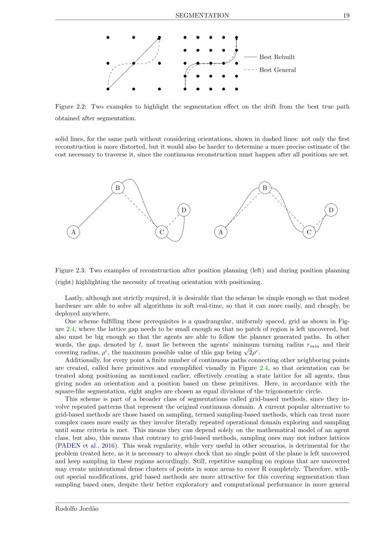
The segmentation scheme chosen is required to fulfill three requirements. First, conserve the originalcost, demand and covering aspects of the original continuous problem. Second, and minimize inherentsegmentation error between the best arbitrary continuous path and the best discretized path, the SimplePath Drift (SimPaD), which is illustrated with examples in Figure 2.2, where the difference between thetrue best path becomes more pronounced as the lattice is made coarser.
Third, any segmentation scheme must be aware of orientation during the path making process tocontemplate agents that are non-holomonic and more precisely estimate the cost of operation by any ofthe agents, otherwise, if this account is not made at the segmentation substage, the generated paths costestimates will become hard to predict, or even impossible to follow by non-holomonic agents, beating oneof the advantages of ahead-of-time planning central to this methodology. Figure 2.3 shows the differenceof a continuous path that would be rebuilt solely looking on the previous traversed node of each arcvisited and another rebuilt by planning the orientations of each node along their positions, shown in
Rodolfo Jordao
SEGMENTATION 19
Best General
Best Rebuilt
Figure 2.2: Two examples to highlight the segmentation effect on the drift from the best true path
obtained after segmentation.
solid lines, for the same path without considering orientations, shown in dashed lines: not only the firstreconstruction is more distorted, but it would also be harder to determine a more precise estimate of thecost necessary to traverse it, since the continuous reconstruction must happen after all positions are set.
A
B
C
D
A
B
C
D
Figure 2.3: Two examples of reconstruction after position planning (left) and during position planning
(right) highlighting the necessity of treating orientation with positioning.
Lastly, although not strictly required, it is desirable that the scheme be simple enough so that modesthardware are able to solve all algorithms in soft real-time, so that it can more easily, and cheaply, bedeployed anywhere.
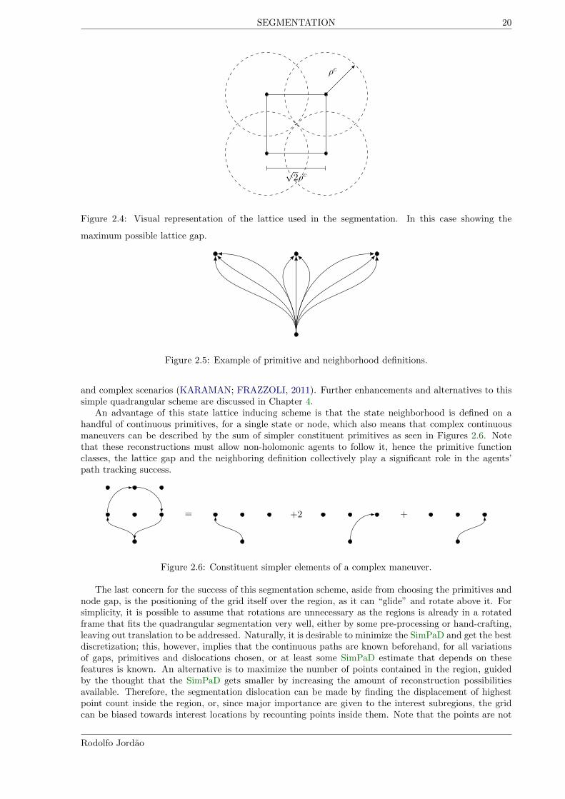
One scheme fulfilling these prerequisites is a quadrangular, uniformly spaced, grid as shown in Fig-ure 2.4, where the lattice gap needs to be small enough so that no patch of region is left uncovered, butalso must be big enough so that the agents are able to follow the planner generated paths. In otherwords, the gap, denoted by l, must lie between the agents’ minimum turning radius rmin and theircovering radius, ρc, the maximum possible value of this gap being
√2ρc.
Additionally, for every point a finite number of continuous paths connecting other neighboring pointsare created, called here primitives and exemplified visually in Figure 2.4, so that orientation can betreated along positioning as mentioned earlier, effectively creating a state lattice for all agents, thusgiving nodes an orientation and a position based on these primitives. Here, in accordance with thesquare-like segmentation, eight angles are chosen as equal divisions of the trigonometric circle.
This scheme is part of a broader class of segmentations called grid-based methods, since they in-volve repeated patterns that represent the original continuous domain. A current popular alternative togrid-based methods are those based on sampling, termed sampling-based methods, which can treat morecomplex cases more easily as they involve literally repeated operational domain exploring and samplinguntil some criteria is met. This means they can depend solely on the mathematical model of an agentclass, but also, this means that contrary to grid-based methods, sampling ones may not induce lattices(PADEN et al., 2016). This weak regularity, while very useful in other scenarios, is detrimental for theproblem treated here, as it is necessary to always check that no single point of the plane is left uncoveredand keep sampling in these regions accordingly. Still, repetitive sampling on regions that are uncoveredmay create unintentional dense clusters of points in some areas to cover R completely. Therefore, with-out special modifications, grid based methods are more attractive for this covering segmentation thansampling based ones, despite their better exploratory and computational performance in more general
Rodolfo Jordao
SEGMENTATION 20
ρc
√2ρc
Figure 2.4: Visual representation of the lattice used in the segmentation. In this case showing the
maximum possible lattice gap.
Figure 2.5: Example of primitive and neighborhood definitions.
and complex scenarios (KARAMAN; FRAZZOLI, 2011). Further enhancements and alternatives to thissimple quadrangular scheme are discussed in Chapter 4.
An advantage of this state lattice inducing scheme is that the state neighborhood is defined on ahandful of continuous primitives, for a single state or node, which also means that complex continuousmaneuvers can be described by the sum of simpler constituent primitives as seen in Figures 2.6. Notethat these reconstructions must allow non-holomonic agents to follow it, hence the primitive functionclasses, the lattice gap and the neighboring definition collectively play a significant role in the agents’path tracking success.
= +2 +
Figure 2.6: Constituent simpler elements of a complex maneuver.
The last concern for the success of this segmentation scheme, aside from choosing the primitives andnode gap, is the positioning of the grid itself over the region, as it can “glide” and rotate above it. Forsimplicity, it is possible to assume that rotations are unnecessary as the regions is already in a rotatedframe that fits the quadrangular segmentation very well, either by some pre-processing or hand-crafting,leaving out translation to be addressed. Naturally, it is desirable to minimize the SimPaD and get the bestdiscretization; this, however, implies that the continuous paths are known beforehand, for all variationsof gaps, primitives and dislocations chosen, or at least some SimPaD estimate that depends on thesefeatures is known. An alternative is to maximize the number of points contained in the region, guidedby the thought that the SimPaD gets smaller by increasing the amount of reconstruction possibilitiesavailable. Therefore, the segmentation dislocation can be made by finding the displacement of highestpoint count inside the region, or, since major importance are given to the interest subregions, the gridcan be biased towards interest locations by recounting points inside them. Note that the points are not
Rodolfo Jordao

COST ESTIMATION 21
the nodes themselves, but points with a orientation attached.To effect this point maximization for a planar region R, let δR(p) be an indicator function that returns
1 if the point p ∈ R2 is in region R and 0 otherwise,
δR(p) =
{1, p ∈ R0, else
, (2.4)
and let d ∈ R2 be the displacement vector in the plane that contains R. Consider all the points that aregenerated by the segmentation scheme in r indexed by the set ip. Then, the positioning maximizationcan be stated as,
maxd∈r2
∑
p∈ipδr (d+ p) . (2.5)
If the bias is to be used, let λ be a positive real number, and δRi a pertinence function for each of theinterest subregions Ri, in the same fashion as δR. Then the optimization problem can be restated as
maxd∈R2
∑
p∈Ip
(δR (d+ p) + λ
∑
i∈IrδRi (d+ p)
), (2.6)
where solutions that do not contain at least one point inside every subregion Ri are discarded,
s.t.∑
p∈IpδRi
(d+ p) > 0, ∀i ∈ Ir (2.7)
Solving (2.6)-(2.7) efficiently requires knowledge of limits for d. Fortunately, these bounds can befound when the quadrangular symmetry of the packaging scheme is considered, so that whenever themesh is moved more than one lattice gap, the same exact mesh is obtained, as exemplified visually byFigure 2.7, where the region R is circular.
dd
Figure 2.7: Example of equivalent lattices achieved via displacement. The left lattice is the original,
the middle lattice is the same as the left one, but displaced diagonally, and the right one is the lattice
obtained by displacing a full diagonal from the left one and half diagonal from the middle one.
Therefore, it is enough to have both displacements be contained in the interval of 0 to the lattice gap,given by l, which is shown in Figure 2.8 by the new position of point A, A’, generated by the displacementd. The final displacement optimization model is thus given by
maxd∈[0,l]2
∑
p∈Ip
(δR (d+ p) + λ
∑
i∈IrδRi (d+ p)
), (2.8)
subject to restriction (2.7).The segmentation results in two entities: the position points themselves in a set N c and a graph
Gc = (N c+, Ec+) named state cell graph, in which the nodes, as defined earlier, are the positions in N c
augmented with a finite set of orientations ϕ ∈ Φ, resulting in the node set N c+ and its connections Ec+.Further possibilities of segmentation are discussed in Chapter 4. Next, the cost estimation of every edgein Ec+ is discussed.
Rodolfo Jordao

COST ESTIMATION 22
A B
CD
lattice gap
d
A’
Figure 2.8: Intervals of search for positioning.
2.3 COST ESTIMATION
To be able to estimate costs between the generated nodes in the segmentation, a representative modelof each agent class is required so prediction of the amount of effort spent between two desired nodes canbe made. As such, some aspects of control and dynamics need to be discussed with their relations to thediscretization.
Alluding established nomenclature from the literature (LAVALLE, 2006; SICILIANO, 2009), thereare mainly two concerning spaces for any description, the operation or trajectory space S, where, as thename implies, all possible trajectories and operations happen, and the configuration space X , where allgeneral information of the agent, such as joint positions, engine thrusts, etc lies. The former, in thiswork, is given by R × [0; 2π], since all trajectories are described by a history of plane positions and anangle of orientation; while the latter can change wildly from agent to agent.
To make these last ideas more formal, consider that an agent a has generalized coordinates q ∈ Xa ⊂Rn that completely describe it, a number of free variables u ∈ Ua ⊂ Rm that works as the input in thesystem, and finally a model fa : R×Xa × Ua → Xa that represents the agent,
q(t) = fa(t, q(t), u(t)), (2.9)
where t ∈ R symbolizes “time” in a context that makes sense for this description. Equation (2.9) is thegeneral form of any agent description in the configuration space, however, the objective is to control theagent trajectory rather than its configuration, i.e. controlling in S rather than in Xa. Thus, every famust be coupled with a transformation, or output, function ha : R×Xa → S,
s(t) = ha(t, q(t)), (2.10)
where s(t) ∈ S for any t ∈ R. Finally, there may be constraints on the agent that forbid it to makeimpossible actions, such as a Unmanned Ground Vehicle (UGV) instantly making a half-turn with zeroradius to backtrack somewhere; represented by the function ga : R×Xa × Ua → R,
0 = ga(t, q(t), u(t)). (2.11)
Equations (2.9) to (2.11) form the basis of any agent description, where the control objective is tomake s(t) follow a predetermined reference path sr(t). It should be remarked that the symbol S wasused here intentionally, to reinforce its relationship with S(bR) from the overall formalization, seeing thatevery sr is, in fact, a member of S(bR) and that R ⊂ S: the symbolism of applying S to a point shouldbe understood as a “filter” function that returns only the continuous paths that start and end at thatpoint, in the same sense, S applied to two different points, S(p1, p2), should be understood as the set ofall continuous paths that start at the first point and end at the second.
Using these definitions for costs estimation, consider a path s ∈ S(pi, pj), for any pi ∈ S and pj ∈ S,a minimum speed vmina and generalized coordinates qa ∈ Xa so that in a time span t ∈ [0;T ], s(t) =ha(t, qa(t)), that is, the agent follows perfectly s in [0;T ] by means of a control ua(t) while respecting its
Rodolfo Jordao
PATH CONSTRUCTION 23
constraints,qa(t) = fa(t, qa(t), ua(t)),
0 = ga(t, qa(t), ua(t)),
|s(t)| > vmina ,
s(t) = ha(t, qa(t)),
(2.12)
the cost function of s, µa(s), is defined as
µa(s) =
∫ T
0
La(ua(t))dt, (2.13)
where La is a strictly positive function that takes the control vector ua and outputs a scalar number, foreach agent class a, representing its cost metric. The minimum speed is a simple mathematical device toincorporate the possibilities of the agent using the environment in its favor when possible, e.g. a UGVgoing down a hill may let its speed increase instead of stopping it. Naturally, unless the agent has perfectenergy savings, or spontaneous energy generation, the cost function is strictly positive for any non-zerocyclic path s starting and ending at any point with minimum speed vmina ,
µa(s) > 0, ∀a ∈ Ia.
Back to segmentation, this continuous cost must be described in terms of nodes and primitives.Consider a path P formed by two neighbor nodes in Gc, (i, ϕi) and (j, ϕj),
P = {(i, ϕi), (j, ϕj)},
and let s be the path formed by the primitive connection between these two nodes as chosen at thesegmentation. The cost of P is then defined to be the cost of s,
µa(P ) = µa(s), (2.14)
and in the same line, the cost variable representing this edge, that is, the weight ci,j,ϕi,ϕj ,a of this edgein Gc, can be defined:
ci,j,ϕi,ϕj ,a = µa(s) = µa(P ) (2.15)
The extension for a discrete path P with higher number of nodes follows the same build-up principleof primitives: for a path P = {(i1, ϕi1), . . . , (in, ϕin)}, the cost is defined as,
µa(P ) =
n−1∑
j=1
µa({(ij , ϕij ), (ij+1, ϕij+1)}), (2.16)
that is, the sum of the individual costs of each neighboring segment present in P . For example, considera path P = {(1, 1), (2, 3), (3, 5), (4, 1)}, then its cost would be the sum of all middle segments:
µa(P ) = c1,4,1,1,a = c1,2,1,3,a + c2,3,3,5,a + c3,4,5,1,a.
2.4 PATH CONSTRUCTION
The ShorPaP can be first enunciated in its continuous form, agreeing with the original continuous PLTAMproblem. For an initial point pi and a final point pf , the problem consists in finding the least costly paths ∈ S(pi, pf ), while having the required minimum speed vmina ,
mins∈S(pi,pf )
µa(s), (2.17)
Rodolfo Jordao

OPTIMAL ASSIGNMENT 24
or, in a more explicit way and closer to what is usually found in optimal control literature (KIRK, 2004),
mins∈S(pi,pf )
∫ T
0
La(ua(t))dt
s.t.
qa(t) = f(t, qa(t), ua(t)),
0 = ga(t, qa(t)),
ha(t, qa(t)) = s(t),
|s(t)| > vmina ,
(2.18)
where all variables preserve the meaning they had previously on (2.12), and for a path that needs to bebuilt knowing the start and end orientations, the constraints function ga would feature this requirement.
Translating this idea into a segmentation-aware form, let P be a variable sized node path with knownstart and end nodes, (i, ϕi) and (f, ϕf ), P = {(i, ϕi), . . . , (f, ϕf )}. The ShorPaP can then be solved byfinding in Gc which nodes minimize the cost between the start and end nodes,
minP⊂Nc+
µa(P ), (2.19)
where all constraints and timing concerns are assumed to be solved by the correct use of lattice gap,primitives choice and positioning. Thus, the computational complexity of computing the solution of(2.18) or (2.17), which usually involve solving a boundary-valued differential partial equation (KIRK,2004), is traded with a graph minimal path problem, which usually involve techniques with known timeand computational resources consumption (CORMEN, 2009).
Two major ways of solving (2.14) is by treating through graph search techniques or modeling it in acombinatorial manner via a Mixed Integer Linear Programming (MILP) model. One big setback of thelatter is that it is computationally difficult: as the size of nodes in Gc grows, there are exponentiallymore possible solutions to seek for a minimum. Problems with this characteristic are usually referred ashaving NP difficulty (CORMEN, 2009), meaning that bigger instances of this problem cannot be solvedwithin reasonable time and computational resources, as of 2018, since the debate of whether P equalsNP still has no solution (WOEGINGER, 2018). Fortunately, the former approach do not suffer from thisdifficulty, and is able to solve this problem optimally, or at least find a very good solution, by looking atthe graph directly and exploiting its connective nature, instead of tackling the combinatorial problem.
For example, he Bellman-Ford algorithm has O(
(dimEc+)2)
, i.e. polynomial worst case complexity
(BELLMAN, 1958), compared to MILP exact methods such as branch-and-bound which have hard toestimate complexities.
The best known ShorPaP solution algorithm to date in a weighted graph, such as Gc, where allweights are positive and no easy guide heuristic is known between any two nodes, is the uniform costsearch algorithm, both eager and lazy versions, the former being commonly known as Dijkstra’s algorithm(FELNER, 2011; DIJKSTRA, 1959). Both are presented here, in Algorithms 1 and 2, respectively, bothbeing orientation-aware for cohesive construction of optimal paths and able to return all shortest pathsfrom a given starting node to any other. Their main differences reside on the trade-off between memoryand processing use: even thought the lazy version would be superior in all ways in a theoretical view(FELNER, 2011), manipulating a list structure takes computational effort, so the total computation timesuffers accordingly, whereas the eager has all nodes already loaded from start. Any variation of thesealgorithms which can efficiently reuse previous computed shortest paths in broader way still did not findwidespread study in the related literature, and may be a research topic on its own.
With the optimal paths coded in values and parents tree, constructing a continuous path is done bystarting from the leaves of the parents tree and backtracking until the starting state is reached. A finalconcern is dealing with bR, due to its out-of-grid nature. The approach used here is to link the “closest”node in N c to bR, thus discarding the need to accommodate an extra orientation exclusively related to bR,then considering that the agents start from this immediate node, rather than in bR itself, subtracting thissmall trip between the immediate node and bR from the agent limit βa. For example, suppose that aftersegmentation is done, the closest node to bR, for agent class a, is i and that the orientation that causesthe least cost from i to bR is ϕi. Then, all agents of class a are considered to start at this states (i, ϕi),while their capacity is reduced by the cost of both going to and from bR, say, termed cR, βa := βa− 2cR.
The results of the path construction stage are the set of all interest points, Nd, and the decisiongraph, Gd = (Nd+, Ed+), which is densely connected by the resulting shortest paths computed. Due tothis dense connection, it follows, for easier posterior treatment, that Nd+ = Nd × Φ.
Rodolfo Jordao

OPTIMAL ASSIGNMENT 25
Algorithm 1 Eager Uniform Cost Search (Dijkstra’s algorithm)
Require: Gc = (N c+, Ec+), a, ci,j,ϕi,ϕj ,a, (is, ϕs)
Q← N × Φ \ {(is, ϕ)|ϕ ∈ Φ}V alues← {(i, ϕ)→∞|∀i ∈ N ;ϕ ∈ Φ}V alues[(is, ϕs)]← 0
Parents← {(i, ϕ)→ −1|∀i ∈ N ;ϕ ∈ Φ}while Q 6= ∅ do
(i, ϕi)←MinimumValue(Q,V alues)
for (j, ϕj) ∈ Neighbors((i, ϕi)) do
if V alues[(j, ϕj)] > V alue[(i, ϕi)] + ci,j,ϕi,ϕj ,a then
V alues[(j, ϕj)]← V alue[(i, ϕi)] + ci,j,ϕi,ϕj ,a
Parents[(j, ϕj)]← (i, ϕi)
end if
end for
Q← Q \ {(i, ϕi)}end while
return V alues, Parents
Algorithm 2 Lazy Uniform Cost Search
Require: Gc = (N c+, Ec+), a, ci,j,ϕi,ϕj ,a, (is, ϕs)
Q← {(is, ϕs)}C ← ∅V alues← {(is, ϕs)]→ 0}Parents← {(i, ϕ)→ ∅}while Q 6= ∅ do
(i, ϕi)← ExtractMinimum(Q,V alues)
C ← C ∪ {(i, ϕi)}for (j, ϕj) ∈ Neighbors((i, ϕi)) \ C do
v ← V alues[(i, ϕi)] + ci,j,ϕi,ϕj ,a
if (j, ϕj) 6∈ Q then
Q← Q ∪ {(j, ϕj)}V alues[(j, ϕj)]← v
Parents[(j, ϕj)]← (i, ϕi)
else if (j, ϕj) ∈ Q and v < V alues[(j, ϕj)] then
V alues[(j, ϕj)]← v
Parents[(j, ϕj)]← (i, ϕi)
end if
end for
end while
return V alues, Parents
Rodolfo Jordao

Mixed Integer Linear Model 26
2.5 OPTIMAL ASSIGNMENT
Consider the set containing all possible cyclic node paths in Gd starting and ending bR, P(bR), thediscrete equivalent of S(bR), The objective is to assign enough cycles P ∈ P(bR) for different agentclasses, a ∈ Ia, satisfying both demand and capacity constraints. One way to systematically treat thisdiscrete combinatorial optimization is through an MILP model.
2.5.1 Mixed Integer Linear Model
Let xi,j,ϕi,ϕj ,a be an integer decision variable that decides how many agents of class a ∈ Ia move from(i, ϕi) ∈ Nd+ to another state (j, ϕj) ∈ Nd+, this integer definition emanating from the fact that agents ofthe same class may have intersecting paths to reach their respective goals. The objective is minimizationof all paths costs,
minx
∑
i∈Nd,j∈Nd
ϕi∈Φ,ϕj∈Φa∈Ia
ci,j,ϕi,ϕj ,axi,j,ϕi,ϕj ,a, (2.20)
with four constraints. First, only connected and cohesive paths, whatever the chosen primitives (Fig-ure 2.9), for every agent class a, are allowed,
∑
i∈Nd
ϕi∈Φ
xi,j,ϕi,ϕj ,a −∑
k∈Nd
ϕk∈Φ
xj,k,ϕj ,ϕk,a = 0, ∀j ∈ Nd;ϕj ∈ Φ; a ∈ Ia. (2.21)
i
j
k
cohesion
i
j
k
cohesion
Figure 2.9: Two different continuous reconstruction with cohesive node links.
Second, all demands must be covered by the agents able to supply that demand visiting the cell,
∑
i∈Nr,a∈Iaϕi∈Φ,ϕj∈Φ
vj,a,oxi,j,ϕi,ϕj ,a ≥ αdj,o, ∀j ∈ Nr; o ∈ Io, (2.22)
where Nr, αdj,o are constructed from Ir, αj,o, and vj,a,o is constructed from µda,o in accordance to thesegmentation scheme, preserving (2.2) demand properties. On the other hand, considering that thedecision graph retains only nodes to be visited, and that the primary function of this demand constraintis to ensure that they are all visited and covered, a further reduction can be made,
∑
i∈Nd,a∈Iaϕi∈Φ,ϕj∈Φ
δa,oxi,j,ϕi,ϕj ,a ≥ δj,o, ∀j ∈ Nd \ {bR}; o ∈ Io, (2.23)
where δa.o is 1 if an agent class a can do some operation and 0 otherwise, the same applies for δj,o inrelation to a node j. This observation removes the necessity to compute and store vj,a,o, α
dj,o for all
interest nodes and operations.
Rodolfo Jordao
Admissible Score Clustering heuristics family 27
For the remaining subtour and capacity constraints, let yi,j,ϕi,ϕj ,a be a variable that represents if anyclass a agent transverses from (i, ϕi) to (j, ϕj), then, it can be defined in relation to x,
yi,j,ϕi,ϕj ,a = min(1, xi,j,ϕi,ϕj ,a) (2.24)
and let PC(bR) be the set of all cyclic paths that do not contain the base. Then, every agent class that isin a cycle without the base must necessarily exit this path to somewhere else, meaning that P ∈ PC(bR)must not sum up to the total of nodes that it contains,
∑
(i,ϕi)∈P(j,ϕj)∈P
yi,j,ϕi,ϕj ,a ≤ dimP − 1, ∀P ∈ PC(bR); a ∈ Ia, (2.25)
and the fourth, capacity constraint,
∑
(i,ϕi)∈Po∈Io
δa,ocni,o +
∑
(i,ϕi)∈Pci,i+,ϕi,ϕi+ ,a
yi,i+,ϕi,ϕi+ ,a≤ βa, ∀P ∈ P(bR); a ∈ Ia, (2.26)
where cni,o is the cost of performing operation o at node i, assuming that the cost of doing the operation isindifferent of the agent doing it, βa are the same limits used in the continuous case, and the sum signifiesa cyclical sequential addition, with i+ being the next node of i in P , i.e. first and second, second andthird, and so on.
Since constraints (2.25) and (2.26) are equivalent to subtour elimination constraints commonly foundin Traveling Salesman Problems (TSPs) and VRPs (GOLDEN; RAGHAVAN; WASIL, 2008; TOTH;VIGO, 2002), it would be possible to replace these for equivalent MTZ (DESROCHERS; LAPORTE,1991) or commodity-flow (LANGEVIN; SOUMIS; DESROSIERS, 1990) constraints. Yet, doing suchmodifications diminishes some computational properties of the MILP model, namely, it makes the relax-ation of the problem itself weaker (TOTH; VIGO, 2002), fixing the best solution obtainable at a marginof the best solution obtainable with the model shown here. Moreover, recent research points out thatthis is true for any MTZ-like constraint, notwithstanding its form (BEKTAS; GOUVEIA, 2014).
Another related restatement, in attempt to ease the exponential number of inequalities, is to includea temporal index τ directly. That is, make x time-aware, xi,j,ϕi,ϕj ,a,τ , which would trade a highernumber of variables for removal of subtour restrictions, since a solution which makes a connected routego unnecessarily backwards certainly is not optimal. Further examination shows that this trade-off cannotin fact be achieved, because every agent is required to start and end its route at the base bR within anytime interval; and that requires the model to have a subtour-elimination alike (2.25) for any time interval,actually increasing the number of constraints.
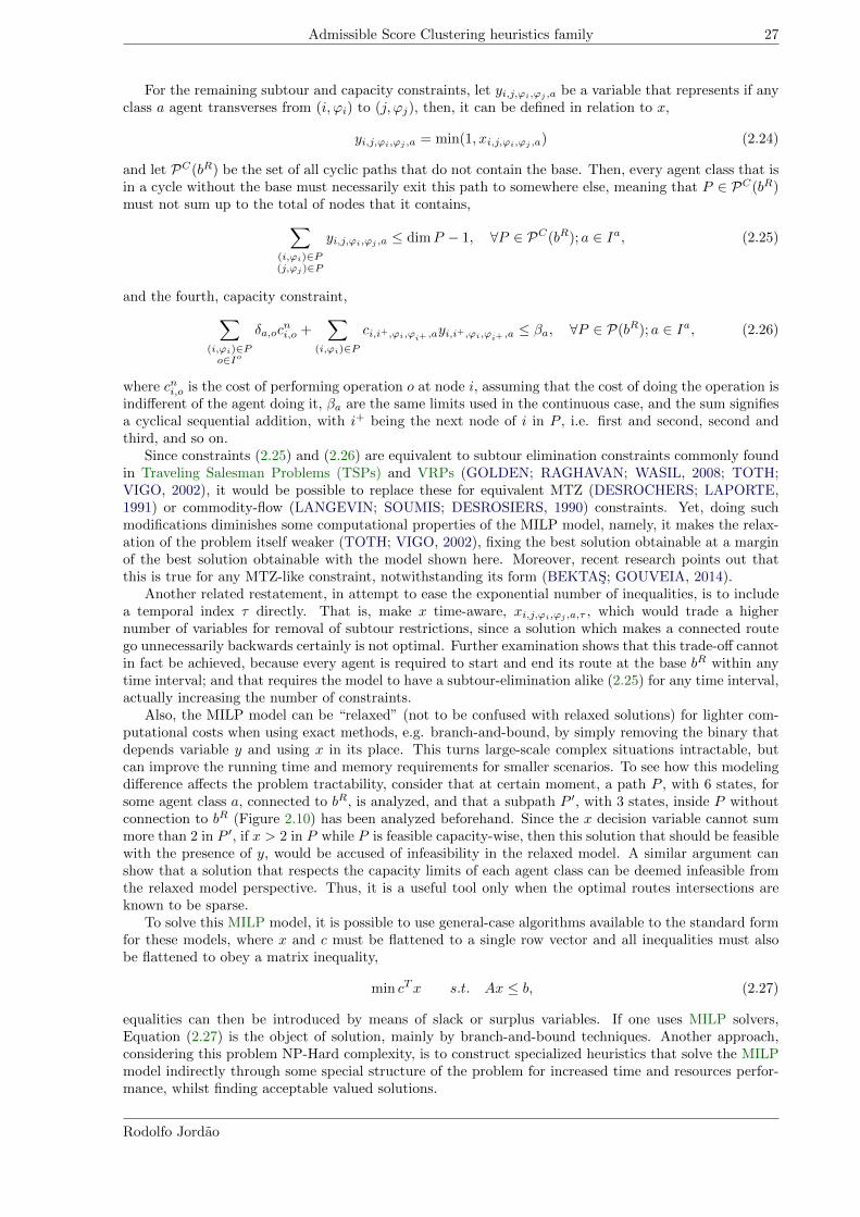
Also, the MILP model can be “relaxed” (not to be confused with relaxed solutions) for lighter com-putational costs when using exact methods, e.g. branch-and-bound, by simply removing the binary thatdepends variable y and using x in its place. This turns large-scale complex situations intractable, butcan improve the running time and memory requirements for smaller scenarios. To see how this modelingdifference affects the problem tractability, consider that at certain moment, a path P , with 6 states, forsome agent class a, connected to bR, is analyzed, and that a subpath P ′, with 3 states, inside P withoutconnection to bR (Figure 2.10) has been analyzed beforehand. Since the x decision variable cannot summore than 2 in P ′, if x > 2 in P while P is feasible capacity-wise, then this solution that should be feasiblewith the presence of y, would be accused of infeasibility in the relaxed model. A similar argument canshow that a solution that respects the capacity limits of each agent class can be deemed infeasible fromthe relaxed model perspective. Thus, it is a useful tool only when the optimal routes intersections areknown to be sparse.
To solve this MILP model, it is possible to use general-case algorithms available to the standard formfor these models, where x and c must be flattened to a single row vector and all inequalities must alsobe flattened to obey a matrix inequality,
min cTx s.t. Ax ≤ b, (2.27)
equalities can then be introduced by means of slack or surplus variables. If one uses MILP solvers,Equation (2.27) is the object of solution, mainly by branch-and-bound techniques. Another approach,considering this problem NP-Hard complexity, is to construct specialized heuristics that solve the MILPmodel indirectly through some special structure of the problem for increased time and resources perfor-mance, whilst finding acceptable valued solutions.
Rodolfo Jordao

Admissible Score Clustering heuristics family 28
bR
P
P ′
Figure 2.10: Example of possible problems with relaxed model limits.
2.5.2 Admissible Score Clustering heuristics family
For problems that resemble VRPs, a viable solution is to first cluster nodes someway and then optimizethe route in this cluster, which consists to solving a local instance of a TSP, effectively separating it intoa general assignment problem coupled with many TSPs. The algorithm developed here, Admissible ScoreClustering (ASC), takes inspiration from tabu-search meta-heuristics (GLOVER, 1986) and other cluster-and-route heuristics already present in the literature (FISHER; JAIKUMAR, 1981). Its conception ismodular and treats routes in the graph directly through transformations in order to achieve betterperformance, making every solution obtained also feasible. Unsurprisingly, graph matching problems,where graph transformations are normally defined and studied, are also NP-hard (ZAGER; VERGHESE,2008). The pseudo-code for general ASC is displayed at Algorithm 3 and its description follows.
Let a tour w be the junction of a path P ∈ P(br) with an agent class a ∈ Ia, w = (P, a). Thestarting solution W is one very far from optimal, composed by single node tours for each of the agentclasses. If this initial solution cannot be made feasible by removal of some tours, the overall problemis infeasible. From this initial solution the main loop starts: all tours are locally optimized as a TSPfollowed by determination of the highest variation feasible transformation T from the transformations setT , (discussion of the local optimization and transforms T are deferred because of their interchangeability),once this best transform, T ∗, is determined and applied, its score is updated according to the solutionvariation. If a local minimum is reached, it is stored if better than the best solution or discarded otherwise,then, a new solution with a random feasible subset of all tours visited so far is built for another iteration,but not before applying a forgetting factor to the scores computed up to that moment. The algorithmsstops if no better solution is attained after maxRepeats local minima were found or maxIters iterationshave elapsed. Here, a simple scoring system which consists of adding one to every tour at every iterationwas used, and the forgetting vector is set to be make all scores lose 1% of their value at each iteration.
Four transforms were defined in this work in a way that they can return favorable variations forevery solution possible; two of these transform are macroscopic transformations while the other two aremicroscopic. Explicitly,
1. Tour Merge: merge in a tail-head fashion two tours from the solution. Illustrated in Figure 2.11.
2. Tour Removal: completely erase a tour from the solution. Illustrated in Figure 2.12.
3. Node Transfer: transfer the nodes between two routes that makes the most cost reduction alongtheir reorientation. Illustrated in Figure 2.13.
4. Node Removal: completely remove a node from a tour in a solution. Illustrated in Figure 2.14.
It must be remarked that the new tours produced by each transform retain the previous agent class,limiting manipulation of classes in use by a solution to tour and node removals. Also, transfer is chosen inplace of insertion as it may result in a favorable transform, whereas insertion would always be unfavorable,requiring special treatment. The following variation deductions, whenever applicable, use the samevariables of the illustrations as a visual aid.
Transference variation applied to two tours w1, w2 in a solution is given by the best sum of nodeinsertion and removal in the direction w1 → w2 or in w2 → w1,
∆transferw1→w2
= mink∈N(w1)
(∆insertionw2,k + ∆removal
w1,k
),
Rodolfo Jordao

Admissible Score Clustering heuristics family 29
Algorithm 3 ASC
Require: Nd, Φ, Ia, c, Constraints, T , maxRepeat
W ← InitialSolution(Nd, Φ, Ia, c, Constraints)
Scores← ∅repeat← 0
W best ←W
Tours← {representation(w)→ w|w ∈W}while repeat < maxRepeat do
for w ∈W do
w ← TourOptimization(w, c)
Tours[representation(w)]← w
end for
score← 0
Wnext ←W
T ∗ ← Identity
for T ∈ T do
∆T , WT ← T (W,Φ, c)
scoreT ← ApplyScore(∆T , T,W,WT , Scores)
if score < scoreT and Constraints(WT ) then
Wnext ←WT
T ∗ ← T
score← scoreT
end if
end for
if score > 0 then
Scores← UpdateScores(T ∗,W,Wnext, Scores)
W ←Wnext
else
if SolutionValue(W ) < SolutionValue(W best) then
repeat← 0
W best ←W
end if
repeat← repeat+ 1
W ← ∅while not Constraints(W ) do
W ←W ∪Random(Tours)
end while
end if
Scores← ForgetScores(Scores)
end while
return W best
Rodolfo Jordao

Admissible Score Clustering heuristics family 30
bR
(i, ϕi)
1
(j, ϕj)
2
Merge 1→ 2
bR
(i, ϕi) (j, ϕj)
1 + 2
Figure 2.11: Illustration of the tour merge transformation.
bR1 2
Removal 2
bR1 2
Figure 2.12: Illustration of the tour removal transformation.
bR
(i, ϕi)
(j, ϕj)
1(k, ϕk)
2
Best 1→ 2Transfer
bR(i, ϕi)
(j, ϕj)
1(k, ϕ′
k)
2
Figure 2.13: Illustration of the node transfer transformation.
Rodolfo Jordao

Admissible Score Clustering heuristics family 31
bR
1
2
3
4
Node 1Removal
bR
1
2
3
4
Figure 2.14: Illustration of the node removal transformation.
whereN is a function that returns the ordered node set from a tour, i.e. N(w) ⊂ Nd, and the minimizationaligns with the search for the most favorable (most negative) transform. Now, the insertion variation foradding a node k in w, is given by subtracting the edge that existed before insertion and summing mostfavorable state addition in the route w with agent class a,
∆insertionw,k = min
ϕk∈Φ(ci,k,ϕi,ϕk,a + ck,j,ϕk,ϕj ,a)− ci,j,ϕi,ϕj ,a,
while removal variation of a node k is simply computed by subtraction of the edges that were in the tourbefore-hand and sum of the new formed edge in the route w with agent class a,
∆removalw,k = ci,j,ϕi,ϕj ,a − (ci,k,ϕi,ϕk,a + ck,j,ϕk,ϕj ,a).
For a tour w with path P and agent class a to be removed from any solution W , the variation isnaturally subtraction of its cost,
∆removalw = −µa(P ),
whereas merge cost variation is given by the minimum of two possible head-tail combinations for twomerging tours w1, w2 ∈W . Let (i, ϕi) be the final state of w1 before the base state (br, ϕb), and let (j, ϕj)be the state of w2 just after base exit (bR, ϕb); the variation of this cost is given by,
∆mergew1→w2
= ci,j,ϕi,ϕj ,a − (ci,bR,b,ϕb,a + cbR,j,ϕi,ϕj ,a),
merge direction w2 → w1 is defined symmetrically.Regarding local tour optimization, one possibility is to solve the orientation-aware TSP MILP model
directly, where techniques prevalent in the literature could be adapted to accommodate orientations. Heretwo heuristics where tested, one inspired by ASC itself and one faintly based on Ant Colony heuristics(DORIGO; BLUM, 2005) and construction methods. The former, named Order and Orientation Switch-ing (OOS) is shown in Algorithm 4, with its transforms T w consisting of reordering states or reorientingthem, while the latter, named Restarting Sequential Construction (ReSC) is shown in Algorithm 5 andconsists in choosing two starting states randomly and trying to construct the best tour possible basedon this starting tour, both local heuristics make use of scoring for local attractor escaping. The ReSCconnection with Ant Colony Heuristics is given by its constructive nature and the scoring system: likepheromones, the scores guide the balance between exploration and exploitation of the local optimization,but also are forgotten as the procedure goes on, just like the pheromones become less pronounced.
Likewise T required explicit computation in ASC, acquiring the costs for T w is a necessity for OOS;but since reorientation is a rather simple transform, only node switching is enunciated next. Switchingrequires consideration of two separate cases: whether they are follow-ups in their tour or not. If they arenot, let (i, ϕi) and (j, ϕj) be states of w and assume without loss of generality that i comes first than jin w; let (i−, ϕ−i ) and (j−, ϕ−j ) be preceding states of i and j, similarly define i+ and j+. The variation
∆switchi,j is given by:
∆switchj→i = min
ϕ′j∈Φ
(ci−,j,ϕ−i ,ϕ′j ,a
+ cj,i+,ϕ′j ,ϕ+i ,a
)−(ci−,i,ϕ−i ,ϕi,a
+ ci,i+,ϕi,ϕ+i ,a
),
∆switchj→i = min
ϕ′i∈Φ
(cj−,i,ϕ−j ,ϕ′i,a
+ ci,j+,ϕ′′i ,ϕ+j ,a
)−(cj−,j,ϕ−j ,ϕj ,a
+ cj,j+,ϕj ,ϕ+j ,a
),
Rodolfo Jordao

Admissible Score Clustering heuristics family 32
Algorithm 4 OOS
Require: w, Φ, c, T w, maxRepeats
Scores← ∅repeat← 0
wbest ← w
while repeat < maxRepeat do
score← 0, wnext ← w, T ∗ ← Identity
for T ∈ T w do
∆T , wT ← T (w,Φ, c)
scoreT ← ApplyScore(∆T , T, w,wT , Scores)
if score < scoreT then
wnext ← wT
T ∗ ← T
score← scoreT
end if
end for
if score > 0 then
Scores← UpdateScores(T ∗, w, wnext, Scores)
w ← wnext
else
if TourValue(w) < TourValue(wbest) then
repeat← 0
wbest ← w
end if
repeat← repeat+ 1
w ← Shuffle(w)
end if
Scores← ForgetScores(Scores)
end while
return wbest
Rodolfo Jordao

Admissible Score Clustering heuristics family 33
Algorithm 5 ReSC
Require: w, Φ, c, maxRepeats
Scores← ∅repeat← 0
wbest ← w
N ← ExtractNodes(w)
while repeat < maxRepeat do
Nw ← N
wnext ← {(bR, ϕbR),RandomState(N,Φ)}while Nw 6= ∅ do
wnext ← BestAddition(wnext, Nw, c, Scores)
Nw ← Nw \ wScores← UpdateScores(wnext, Scores)
end while
if TourValue(w) < TourValue(wbest) then
repeat← 0
wbest ← w
end if
repeat← repeat+ 1
Scores← ForgetScores(Scores)
end while
return wbest
Rodolfo Jordao

IMPLEMENTATION ASPECTS 34
∆switchi,j = ∆switch
j→i + ∆switchi→j .
Otherwise, if i+ = j and i = j−, then due to their path overlap,
∆switchi,j = min
ϕ′i∈Φϕ′j∈Φ
(ci−,j,ϕ−i ,ϕ′j ,a
+ cj,i,ϕ′j ,ϕ′i,a + ci,j+,ϕ′i,ϕ+j ,a
)−(ci−,i,ϕ−i ,ϕi,a
+ ci,j,ϕi,ϕj ,a + cj,j+,ϕj ,ϕ+j ,a
).
2.6 IMPLEMENTATION ASPECTS
The positioning for segmentation, that is, Equation (2.6), is done via simple linear searches, as theyprovide a balance between ease of implementation, light computational cost and solution accuracy; thisbalance regulated by the amount of partitions made in the search interval.
The pertinence function for R, δR, can be computed in two ways. If R (or any Ri) is already definedthrough a function g,
R = {x ∈ R2 | g(x) ≤ 0}then it is just a matter of computing the value of g given a desired p to be check for region R. Otherwise,if the shape R is defined by many boundary nodes connected by straight lines, a different approach isnecessary to correctly test if p is inside R. A fairly general and efficient algorithm is a specialized formof ray casting: from each candidate point p, a half-line is drawn to either left or right. Let crosses bethe number of boundaries crosses the half-line made in the region R, then if crosses is an odd number,the point p is inside the region, otherwise, it is outside (Figure 2.15). This method also works to checkthe former function-defined boundary; and while this is theoretically correct, simply using p directly withg greatly improves performance over any other algorithmic method. Asymptotically speaking, the raycasting algorithm is, at least, of linear complexity on the size of boundary nodes; while direct evaluationis always constant in complexity, i.e O(n) vs O(1), where O({) is the class of functions that are majoredby f (CORMEN, 2009; APOSTOL, 2007). An efficient implementation is available in Algorithm 6.
1: inside
3: inside
2: outside
2: outside
Figure 2.15: Ray casting algorithm visualization.
Those versed in convex optimization may question the existence of some better search tool in caseR is a convex shape. Due to the discrete nature of the optimization problem, with many instantaneousoscillations in value, even with a convex region R any guided search method that does not go through, in aresolution-wise sense, the whole displacements domain, is likely to fail finding the cloud point optimizationglobal solution. Figure 2.17 shows a very simple convex region R, covered with circles of radius ρc = 0.5,along resulting values of δR for some variations in the displacement vector d; and the entanglementobserved shows the existence of valleys even for simple shapes.
Also, since only the nodes inside R are necessary, a check-up can be made at the segmentation sectionwhich retains only the points that are inside R for path construction and consequently assignment. Thepertinence function δR can be used as a filter once (2.6)-(2.7) is solved, resulting in a lower sized graphwith coverage as exemplified by Figure 2.17. Possible spots not covered can be made covered by a latticerefinement in the specific region that contains the spot.
Rodolfo Jordao

IMPLEMENTATION ASPECTS 35
Algorithm 6 Polygon pertinence ray casting algorithm
Require: point p, Boundary B.
inside← False
for pB ∈ B do
p′ ← NextBoundaryPoint(B, pB) . Get succeeding point in the boundary list
if pBy < py < p′y then . check if y-coord. of p is between those of pB and p′
xref =(p′x − pBx )
(p′y − pBy )(py − pBy ) + pBx . Subscripts are axes access.
if |xref − px| < tolerance then
return True . if the x coord. is right on the ref. Then its part of the polygon.
else if xref < px then
inside← ¬inside . else keep looping and counting.
end if
end if
end for
return inside
ReferenceNode
StartNode
R
dx
dy
ρc = 0.5
5
8
−0.25 −0.2 −0.15 −0.1 −0.05 0
255
260
265
270
275
dy
∑δ R
dx = −0.5000dx = −0.4875dx = −0.4650dx = −0.4375
Figure 2.16: Simple convex region and its segmentation objective function.
Filter
Figure 2.17: Result of filtering for interest nodes after segmentation.
Rodolfo Jordao

IMPLEMENTATION ASPECTS 36
Lastly, a minor possible optimization for the ASC is to simply check specific constraints after eachspecific transform is executed. For instance, tour removal may violate demand constraint but neverthe capacity constraint, whereas merge and transfer may violate the capacity constraint, but never thedemand constraint.
Rodolfo Jordao

37
3 VALIDATION AND RESULTS
3.1 CASE STUDIES
Four missions have been created to test out the merits of this methodology, since there is still a shortageof benchmarks and standardized tests for problems reasonably similar to PLTAMs. All of them havethe same underlying region and working agent classes, their main difference being capacity and demandconstraints. They are shown in Table 3.1.
Table 3.1: Case studies considered.
Case Interests Obstacles Description Capacity
1 1 Small None Small region to be covered by first operation.UGV: 100
UAV: 100
2 2 Small 1 Big central One small region is almost unreachable to UGVs.UGV: 100
UAV: 100
32 Small
1 Big1 Big central One small region is almost unreachable to UGVs.
UGV: 100
UAV: 100
4 2 Medium 1 Big central Both agents have very tight capacity limits.UGV: 22
UAV: 40
The first and simplest case study is designed to show all the steps of the planner visually. The second isdesigned to test out the inherent obstacle avoidance of the known map and exercise cooperation betweenthe agents. The third is designed to test out local optimization influence on the solution along agentcooperation. The fourth and last one is designed to test out cooperation and task distribution betweenthe agents, since they have tight capacity limits.
The agent classes are represented by corpuscular entities, one that is a UGV,
Mgroundv(t) = −bgroundv(t) + u(t),
where v is the velocity vector, Mground and bground are parameters representing lumped inertias andlosses, respectively. Velocity damping is a natural lump simplification of terrain effects upon the agent’smovement, making it lose momentum, otherwise, without any energy input, the agent would move forwardperpetually. The other agent class is a UAV,
Mairv(t) = −bairv(t) + bwindw(t) + u(t),
where w is the wind velocity vector, presumably almost constant during operation, and bwind is thelumped wind effect on the UAV, all other variables having equal significance to the UGV. This additionrepresents in a simple way the wind compliance of a general UAV. The model numerical parameterschosen are displayed in Table 3.2 along the operations each agent class is able to do. In essence, theseparameters were chosen to ensure that UGVs have cheaper operation costs than UAVs, while only UAVscan access every area of the map.
Explicitly, the missions attempt to study two major aspects of the planning methodology in additionto demonstrating the workings of the planner: cooperation between the different agent classes to achievethe demand goal, and distribution between agents of the same class to circumvent capacity limitations.

SIMULATION RESULTS 38
Table 3.2: Agent classes definitions
Agent Parameters Operations
UGVMground = 1.0
bground = 0.11, 2
UAV
Mair = 2.0
bair = 0.05
bwind = 0.1
w(t) = [−1, 0]T
2
These four missions were solved either by exact techniques, as defined by branch-and-bound based oneswith lazily instanced constraints, via the commercial GUROBI solver (GUROBI OPTIMIZATION, 2016),and by two heuristics from the ASC family discussed earlier: ASC+OOS and ASC+ReSC. Hardware andsoftware-wise, all overall programs were coded in the open-source language Julia, except by the GUROBIsolver which is closed-source, and ran in a common desktop computer. It should also be noted that therelaxed model was used for the exact methods, since preliminary tests without relaxation ran for morethan 10 hours without finding their respective solution and that these proposed initial tests have relativelysmall cover and demand area, making them unlikely to show the intractability discussed in Section 2.5.1.Finally, the stopping criteria for the heuristics used were 300 iterations for the ASC overall, allowing upto 10 local minimum repetitions, and 100 iterations for any local optimization algorithm, allowing again10 local minimum repetitions before stopping.
3.2 SIMULATION RESULTS
The aggregated results from these solutions can be seen in Table 3.3, with descriptive statistics from 100heuristic techniques runs and 15 exact technique runs. Additionally, Figures 3.1 through 3.8 show atleast one solution for each case covered, remarking that the exact and heuristic solutions for cases 1 and2 were identical.
Figures 3.1 to 3.4 show all the steps the planner did for case 1 in a demonstrative fashion; startingin the segmentation stage, filtering the interest points, building the shortest paths and finally solvingthe assignment problem to find the solution. Note that the paths showed for the construction stage(Figure 3.3) are a sample of the total found best paths between the two interest nodes. The second case(Figure 3.5) serves as an example of the obstacle avoidance feature of the planner, by means of pathcost invalidation for any such paths that traverse an obstacle for that particular agent class, as seen inthis case, where the UGV detours from its optimal path found in case 1 because of the central obstacle,whereas the UAV moves without problems over this same obstacle for a interest region inside it. Again,the resulting solution is identical via both heuristic and exact methods. The other two cases (Figures 3.6to 3.9) have bigger scales and can be subject to further analysis.
Visually, it can be seen from all Figures representing the solutions that this planner was successful onits objective for creating collaborative continuous paths for the agents. Second, the exact solutions showsthat coverage patterns usually set a priori, such as swiping, appear naturally on the reconstructed tours,although the agents exit out of the swipe motion early for increased cost economy while still retainingdemand coverage, as evidenced particularly in Figure 3.9.
Some numerical properties of the model and techniques used can be observed from the collecteddata. For the cooperation mission, where the capacity constraint is greatly relaxed and far from optimalsolutions with a single tour for each agent class are easily feasible, exact methods can find the final solutionquickly, with about 33% gain in mean time against the two heuristics used, while having 13% and 20%gain in mean optimum value (including tasks costs). On the other hand, the distribution mission, wherethe capacity was tight and far from optimal tours would be infeasible, exact methods ran for much longerthan the heuristics, the mean running time of the former being at least 12500% of the latter, whereas
Rodolfo Jordao

SIMULATION RESULTS 39
−1 0 1 2 3 4 5 6 7 8 9 10 11
−5
−4
−3
−2
−1
0
1
2
3
4
5
6
7
8
9
10
11
12
13
bR
X [space unit]
Y[space
unit]
Figure 3.1: Point cloud and cell graph of case 1.
Rodolfo Jordao

SIMULATION RESULTS 40
−1 0 1 2 3 4 5 6 7 8 9 10 11
−5
−4
−3
−2
−1
0
1
2
3
4
5
6
7
8
9
10
11
12
13
bR
X [space unit]
Y[space
unit]
Figure 3.2: Filtered interest nodes for case 1 with their covering radii.
Rodolfo Jordao

SIMULATION RESULTS 41
−1 0 1 2 3 4 5 6 7 8 9 10 11
−5
−4
−3
−2
−1
0
1
2
3
4
5
6
7
8
9
10
11
12
13
bR
X [space unit]
Y[space
unit]UAVUGV
Figure 3.3: Sample of all constructed paths for case 1.
Rodolfo Jordao

SIMULATION RESULTS 42
−1 0 1 2 3 4 5 6 7 8 9 10 11
−5
−4
−3
−2
−1
0
1
2
3
4
5
6
7
8
9
10
11
12
13
bR
X [space unit]
Y[space
unit]
Tour 1, Agent UGV
Figure 3.4: Resulting tours for exact and ASC solutions of case 1.
Rodolfo Jordao
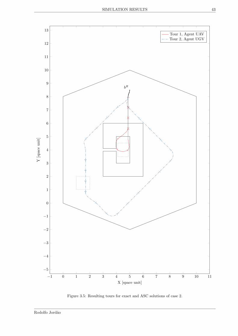
SIMULATION RESULTS 43
−1 0 1 2 3 4 5 6 7 8 9 10 11
−5
−4
−3
−2
−1
0
1
2
3
4
5
6
7
8
9
10
11
12
13
bR
X [space unit]
Y[space
unit]
Tour 1, Agent UAVTour 2, Agent UGV
Figure 3.5: Resulting tours for exact and ASC solutions of case 2.
Rodolfo Jordao

SIMULATION RESULTS 44
−1 0 1 2 3 4 5 6 7 8 9 10 11
−5
−4
−3
−2
−1
0
1
2
3
4
5
6
7
8
9
10
11
12
13
bR
X [space unit]
Y[space
unit]
Tour 1, Agent UAVTour 2, Agent UGV
Figure 3.6: Resulting tours for a ASC+OOS solution of case 3.
Rodolfo Jordao
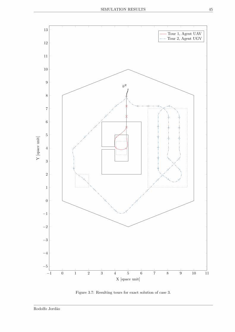
SIMULATION RESULTS 45
−1 0 1 2 3 4 5 6 7 8 9 10 11
−5
−4
−3
−2
−1
0
1
2
3
4
5
6
7
8
9
10
11
12
13
bR
X [space unit]
Y[space
unit]
Tour 1, Agent UAVTour 2, Agent UGV
Figure 3.7: Resulting tours for exact solution of case 3.
Rodolfo Jordao

SIMULATION RESULTS 46
−1 0 1 2 3 4 5 6 7 8 9 10 11
−5
−4
−3
−2
−1
0
1
2
3
4
5
6
7
8
9
10
11
12
13
bR
X [space unit]
Y[space
unit]
Tour 1, Agent UGVTour 2, Agent UGV
Figure 3.8: Resulting tours for a ASC+OOS solution of case 4.
Rodolfo Jordao
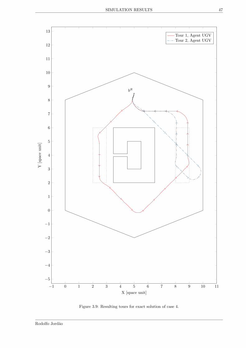
SIMULATION RESULTS 47
−1 0 1 2 3 4 5 6 7 8 9 10 11
−5
−4
−3
−2
−1
0
1
2
3
4
5
6
7
8
9
10
11
12
13
bR
X [space unit]
Y[space
unit]
Tour 1, Agent UGVTour 2, Agent UGV
Figure 3.9: Resulting tours for exact solution of case 4.
Rodolfo Jordao

SIMULATION RESULTS 48
Table 3.3: Solution Value and timing.
Case Purpose Sol. Method Best Value Mean Value Mean Time [s]
1 Steps ASC+OOS 11.88 – 1.12× 10⁻³ ± 2.05× 10⁻⁴
1 Steps ASC+ReSC 11.88 – 1.11× 10⁻³ ± 2.10× 10⁻⁴
1 Steps Exact-Relaxed 11.88 – 9.00× 10⁻³ ± 1.66× 10⁻⁴
2 Collision ASC+OOS 27.35 – 1.12× 10⁻² ± 7.04× 10⁻³
2 Collision ASC+ReSC 27.35 – 1.24× 10⁻² ± 1.92× 10⁻²
2 Collision Exact-Relaxed 27.35 – 2.69× 10⁻² ± 4.43× 10⁻⁴
3 Cooperation ASC+OOS 50.48 56.31± 2.05 20.20± 5.13
3 Cooperation ASC+ReSC 59.04 66.63± 1.32 15.53± 6.12
3 Cooperation Exact-Relaxed 45.12 – 13.60± 1.12
4 Distribution ASC+OOS 33.04 35.71± 0.59 4.83± 1.28
4 Distribution ASC+ReSC 33.57 41.83± 3.16 3.15± 0.76
4 Distribution Exact-Relaxed 33.04 – 606.44± 20.06
one of the heuristics actually achieved the global optimum, having mean suboptimal values standingat about 18% of the global optimum. Hence, it can be seen through these cases that the capacityrestriction place the greatest burden on solution techniques for the problem, specially exact generalmethods, demanding more resources and solution time as the capacity contribution gets more pronounced.ASC’s heuristics as proposed here, treats these restrictions naturally via direct tour manipulation, thusretain performance despite tight capacity restrictions. However, the heuristics saw worse performancewhen dealing with dense regions; a situation that can be remedied by parameters and local optimizationalgorithm change. Additionally, ASC+ReSC found worse solutions overall, notwithstanding general goodresults of probabilistic constructive methods in the literature, such as Ant Colony Heuristics. This canbe attributed to the ASC itself, since its operations are more akin to ordering than to building, makingoptimizers like OOS a natural fit. Finally, it becomes clearer that exact methods are more likely to failin giving any solution at all for bigger instance, since these results were obtained with the relaxed model,which lose representation intrinsically on large-scale situations.
Aside from time and value, some implementations of this methodology may also require memorybounds for the algorithms. Because Julia, which is a Garbage collected language, was selected for this workof prototypical nature, memory estimates may not represent the best possible hardware resource economy,as well as the times obtained may also be reduced by code optimization and native implementation.Nevertheless, by sampling the operational system monitor on some tests, ASC’s attained a maximumof 300 Mb memory consumption, while the GUROBI solver attained as much as 3 Gb of memory. Itis expected that by implementing the solver on compiled and highly optimized language environments,such as C++ or FORTRAN, the resource usage and heuristic solution time will decrease and increase,respectively, favorably.
These tests, their code and instructions for using them are available at a public web repository madeby the authors (JORDAO, 2018) for this work.
Rodolfo Jordao
49
4 CONCLUSION AND FUTURE WORKS
A Methodology tackling Persistent Long Term Autonomous Missions for cooperative autonomous vehicles,consisted of heurisitcs able to plan ahead of time all agents’ orders, was presented based on a newformalization that reduces the overall problem to a path construction and a combinatorial optimizationproblem and four case studies were proposed and solved for validation purposes.
The methodology designed is able to successfully produce acceptable continuous routes and tasks forthe agents in questions. Moreover, its modular nature enables further studies on other realizations, withdifferent segmentations into topological maps or different solving methodologies with other heuristics andimplementations. Some possible improvements follow.
It is within the authors’ opinion that the ASC heuristics family is, at least, asymptotically optimal,observing that the bad initial solution can possibly generate every other solution through admissibletransformations and its performance can be highly-tuned by change of the local optimization heuristicand scoring system. Confirmation or dismissal of this claim, along with modifications that include seedgeneration for faster runs is left for future works. Regarding segmentation, a more hierarchical schemecan be used, by shrinking each interest subregion into a single entity with many possible entrances andexists, while the internal cost could be solved with cost transforms commonly used in pure coverageproblems. The downside of this change is that the costs of demand coverage in these subregions may risedue to the fixed internal trajectories.
Also, the MILP model may be changed to include only the maximum cost of path operations, insteadof their sum; effectively making a single path for same class agents with different tasks, but also requiring asecond optimization procedure for dividing said tasks optimally. Additionally, the methodology is alreadygeneral enough to accommodate non-uniform segmentation schemes, through better use of index sets andbroader definition of states for each agent, but then also requiring treatment of sampling schemes as someof the previous works mentioned. For instance, only interest regions can be segmented in a regular basis,whereas the outer non-interest regions can be sampled according to some criteria, say, better SimPaDminimization other than point counting, and then connected via general ShorPaPs, culminating in ahybrid segmentation scheme.
Some remarks can be made about the up and downsides of the methodology realization as presentedhere. It is apparent that although optimality can be checked and achieved systematically via optimiza-tion, if the agents’ models change quicker than the mean tour designed by the planner, by environmentinteraction or hardware degradation, the cost estimate becomes increasingly worse; thus, this realization,as presented, is more suited to missions with slow environmental changes, good a priori knowledge ofthe mission region and missions that need direct treatment of agents with expressive non-holomonic con-straints. Yet, the only major communication required for success of this long term planning is betweenbase and agent, during this agent visit to the operations base, possibly lowering the hardware costs ofthe mission and also promoting fault tolerance in case of communication breakdown.
Robustness can be achieved by closing an information loop between the agents knowledge of the mapthrough their traversal and the planner current knowledge, as mentioned briefly in Chapter 1. Thusupdating the real cost of every tour component after each route is complete, for each agent. Such courseis more pertinent to a full integration of the planner with every agent, and is left for future works.
Finally, once these suggestions of improvements are followed, another line of expansion is the use ofbetter models for agents’ cost estimation, or even more classes of agents, other than corpuscular entities.Even though this possibility was already covered by the principle of interchangeability of the estimators,the effective change and possible use of more descriptive models, along with real hardware tests, wouldprovide stronger validation for this methodology.

50
Bibliography
APOSTOL, Tom M. Calculus, Volume I. [S.l.]: John Wiley & Sons, 2007. v. 1.
BEKTAS, Tolga; GOUVEIA, Luis. Requiem for the Miller-Tucker-Zemlin Subtour Elimination
Constraints? European Journal of Operational Research, v. 236, n. 3, p. 820–832, 2014. ISSN
03772217. DOI: 10.1016/j.ejor.2013.07.038.
BELLMAN, Richard. On a Routing Problem. Quarterly of Applied Mathematics, v. 16, n. 1,
p. 87–90, 1958. ISSN 0033-569X, 1552-4485. DOI: 10.1090/qam/102435.
BENTZ, William; HOANG, Tru; BAYASGALAN, Enkhmurun; PANAGOU, Dimitra. Complete 3-D
Dynamic Coverage in Energy-Constrained Multi-UAV Sensor Networks. Autonomous Robots,
p. 1–27, 26 July 2017. ISSN 0929-5593, 1573-7527. DOI: 10.1007/s10514-017-9661-x.
BIRCHER, Andreas; KAMEL, Mina; ALEXIS, Kostas; BURRI, Michael; OETTERSHAGEN, Philipp;
OMARI, Sammy; MANTEL, Thomas; SIEGWART, Roland. Three-Dimensional Coverage Path
Planning via Viewpoint Resampling and Tour Optimization for Aerial Robots. Autonomous Robots,
v. 40, n. 6, p. 1059–1078, 1 Aug. 2016. ISSN 0929-5593, 1573-7527. DOI: 10.1007/s10514-015-9517-1.
BOCCALATTE, Marco; BROGI, Filippo; CATALFAMO, Francesco; MADDALUNO, Stefania;
MARTINO, Michele; MELLANO, Valter; ROSAZZA PRIN, Paolo; SOLITRO, Filomena;
TORASSO, Pietro; TORTA, Gianluca. A Multi-UAS Cooperative Mission Over Non-Segregated Civil
Areas. Journal of Intelligent & Robotic Systems, v. 70, p. 275–291, 1-4 Apr. 2013. ISSN
0921-0296, 1573-0409. DOI: 10.1007/s10846-012-9706-5.
BRODERICK, John A.; TILBURY, Dawn M.; ATKINS, Ella M. Optimal Coverage Trajectories for a
UGV with Tradeoffs for Energy and Time. Autonomous Robots, v. 36, n. 3, p. 257–271, 1 Mar. 2014.
ISSN 0929-5593, 1573-7527. DOI: 10.1007/s10514-013-9348-x.
BURGER, Mernout; HUISKAMP, Marco; KEVICZKY, Tamas. Complete Field Coverage as a
Multi-Vehicle Routing Problem. IFAC Proceedings Volumes, v. 46, n. 18, p. 97–102, Aug. 2013.
ISSN 14746670. DOI: 10.3182/20130828-2-SF-3019.00050.

Bibliography 51
CAMPOS, V.; MOTA, E. Heuristic Procedures for the Capacitated Vehicle Routing Problem.
Computational Optimization and Applications, v. 16, n. 3, p. 265–277, Sept. 2000. ISSN
0926-6003, 1573-2894. DOI: 10.1023/A:1008768313174.
CORMEN, Thomas H. Introduction to Algorithms. [S.l.]: MIT press, 2009.
DAMILANO, Luca; GUGLIERI, Giorgio; QUAGLIOTTI, Fulvia; SALE, Ilaria; LUNGHI, Alessio.
Ground Control Station Embedded Mission Planning for UAS. Journal of Intelligent & Robotic
Systems, v. 69, p. 241–256, 1-4 Jan. 2013. ISSN 0921-0296, 1573-0409. DOI:
10.1007/s10846-012-9697-2.
DESROCHERS, Martin; LAPORTE, Gilbert. Improvements and Extensions to the
Miller-Tucker-Zemlin Subtour Elimination Constraints. Operations Research Letters, v. 10, n. 1,
p. 27–36, 1991.
DIJKSTRA, E. W. A Note on Two Problems in Connexion with Graphs. Numerische Mathematik,
v. 1, n. 1, p. 269–271, Dec. 1959. ISSN 0029-599X, 0945-3245. DOI: 10.1007/BF01386390.
DORIGO, Marco; BLUM, Christian. Ant Colony Optimization Theory: A Survey. Theoretical
Computer Science, v. 344, n. 2, p. 243–278, 17 Nov. 2005. ISSN 0304-3975. DOI:
10.1016/j.tcs.2005.05.020.
ELFES, ALBERTO; BUENO, Samuel S.; BERGERMAN, Marcel; RAMOS, Josua Jr. G.;
GOMES, Sao Bittencourt Varella. Project AURORA: Development of an Autonomous Unmanned
Remote Monitoring Robotic Airship. Journal of the Brazilian Computer Society, v. 4, Apr. 1998.
ISSN 0104-6500.
FAZLI, Pooyan; DAVOODI, Alireza; MACKWORTH, Alan K. Multi-Robot Repeated Area Coverage.
Autonomous Robots, v. 34, n. 4, p. 251–276, 1 May 2013. ISSN 0929-5593, 1573-7527. DOI:
10.1007/s10514-012-9319-7.
FELNER, Ariel. Position Paper: Dijkstra’s Algorithm versus Uniform Cost Search or a Case against
Dijkstra’s Algorithm. In: FOURTH Annual Symposium on Combinatorial Search. [S.l.: s.n.], 2011.
FISHER, Marshall L.; JAIKUMAR, Ramchandran. A Generalized Assignment Heuristic for Vehicle
Routing. Networks, v. 11, n. 2, p. 109–124, 1981. ISSN 10970037. DOI: 10.1002/net.3230110205.
GLOVER, Fred. Future Paths for Integer Programming and Links to Artificial Intelligence.
Computers & operations research, v. 13, n. 5, p. 533–549, 1986.
Rodolfo Jordao
Bibliography 52
GOLDEN, Bruce; RAGHAVAN, S.; WASIL, Edward. The Vehicle Routing Problem: Latest
Advances and New Challenges. [S.l.: s.n.], 2008. v. 43. 589 pp. ISBN 978-0-387-77777-1. DOI:
10.1007/978-0-387-77778-8.
GUROBI OPTIMIZATION, Inc. Gurobi Optimizer Reference Manual. [S.l.: s.n.], 2016.
INPE. PRODES. Sao Jose dos Campos, 2017.
ISAACS, Jason T.; HESPANHA, Joao P. Dubins Traveling Salesman Problem with Neighborhoods: A
Graph-Based Approach. Algorithms, v. 6, n. 1, p. 84–99, 2013. ISSN 19994893. DOI:
10.3390/a6010084.
JAVANMARD ALITAPPEH, Reza; A. S. PEREIRA, Guilherme; R. ARAUJO, Arthur;
C. A. PIMENTA, Luciano. Multi-Robot Deployment Using Topological Maps. Journal of Intelligent
and Robotic Systems: Theory and Applications, v. 86, p. 641–661, 3-4 2017. ISSN 15730409.
DOI: 10.1007/s10846-017-0471-3.
JORDAO, Rodolfo. JordaoRodolfo / PLTAM-2017-Paper-Companion / Admin / Repository
Details — Bitbucket. Available from:
¡https://bitbucket.org/JordaoRodolfo/pltam-2017-paper-companion/admin¿. Visited on: 24 Jan.
2018.
KARAMAN, Sertac; FRAZZOLI, Emilio. Sampling-Based Algorithms for Optimal Motion Planning,
p. 1–76, 2011. ISSN 0278-3649. DOI: 10.1177/0278364911406761.
KIRK, Donald E. Optimal Control Theory: An Introduction. Mineola, N.Y: Dover Publications,
2004. 452 pp. ISBN 978-0-486-43484-1.
LANGEVIN, Andre; SOUMIS, Francois; DESROSIERS, Jacques. Classification of Travelling Salesman
Problem Formulations. Operations Research Letters, v. 9, n. 2, p. 127–132, 1990.
LAVALLE, Steven M. Planning Algorithms. [S.l.]: Cambridge university press, 2006.
MITCHELL, Derek; CORAH, Micah; CHAKRABORTY, Nilanjan; SYCARA, Katia;
MICHAEL, Nathan. Multi-Robot Long-Term Persistent Coverage with Fuel Constrained Robots. In:
PROCEEDINGS - IEEE International Conference on Robotics and Automation. [S.l.: s.n.], 2015.
2015-June, p. 1093–1099. ISBN 978-1-4799-6923-4. DOI: 10.1109/ICRA.2015.7139312.
NASA, JPL. Mars Science Laboratory. Available from: ¡https://mars.nasa.gov/msl/¿. Visited
on: 5 Dec. 2017.
Rodolfo Jordao

CONCLUSION AND FUTURE WORKS 53
PADEN, Brian; CAP, Michal; YONG, Sze Zheng; YERSHOV, Dmitry; FRAZZOLI, Emilio. A Survey
of Motion Planning and Control Techniques for Self-Driving Urban Vehicles, p. 1–27, 2016. ISSN
2379-8904. DOI: 10.1109/TIV.2016.2578706.
PINAGE, Felipe A.; CAVALHO, Jose Reginaldo H.; QUEIROZ-NETO, Jose P. Visual-Based Natural
Landmark Tracking Method to Support UAV Navigation over Rain Forest Areas. In: VISAPP.
[S.l.: s.n.], 2013.
PIVTORAIKO, Mikhail; KNEPPER, Ross Alan; KELLY, Alonzo. Differentially Constrained Mobile
Robot Motion Planning in State Lattices. Journal of Field Robotics, v. 26, n. 3, p. 308–333, Mar.
2009.
SICILIANO, Bruno. Robotics : Modelling, Planning and Control. London: Springer, 2009. ISBN
978-1-84628-642-1.
TOTH, Paolo; VIGO, Daniele. The Vehicle Routing Problem. [S.l.: s.n.], 2002. v. 9. ISBN
0-89871-579-2.
TSOURDOS, Antonios; WHITE, Brian; SHANMUGAVEL, Madhavan. Cooperative Path Planning
of Unmanned Aerial Vehicles. [S.l.: s.n.], 2010.
VIDAL, Thibaut; CRAINIC, Teodor Gabriel; GENDREAU, Michel; PRINS, Christian. A Unified
Solution Framework for Multi-Attribute Vehicle Routing Problems. European Journal of
Operational Research, v. 234, n. 3, p. 658–673, 2014. ISSN 03772217. DOI:
10.1016/j.ejor.2013.09.045.
. Heuristics for Multi-Attribute Vehicle Routing Problems: A Survey and Synthesis.
European Journal of Operational Research, v. 231, n. 1, p. 1–21, 2013. ISSN 03772217. DOI:
10.1016/j.ejor.2013.02.053.
WOEGINGER, Gerhard. The P-versus-NP Page. [S.l.: s.n.], 27 Feb. 2018.
XU, Anqi; VIRIYASUTHEE, Chatavut; REKLEITIS, Ioannis. Efficient Complete Coverage of a Known
Arbitrary Environment with Applications to Aerial Operations. Autonomous Robots, v. 36, n. 4,
p. 365–381, 1 Apr. 2014. ISSN 0929-5593, 1573-7527. DOI: 10.1007/s10514-013-9364-x.
ZAGER, Laura A.; VERGHESE, George C. Graph Similarity Scoring and Matching. Applied
Mathematics Letters, v. 21, n. 1, p. 86–94, 2008. ISSN 08939659. DOI:
10.1016/j.aml.2007.01.006.
Rodolfo Jordao