pipe flow - unimasr · loss in moving water at outlet ... design of single pipe flow ......
TRANSCRIPT

Lecture 17
Pipe Flow

Pipe Flow and the Energy EquationFor pipe flow, the Bernoulli equation alone is not sufficient. Friction loss along the pipe, and momentum loss through diameter changes and corners take head (energy) out of a system that theoretically conserves energy. Therefore, to correctly calculate the flow and pressures in pipe systems, the Bernoulli Equation must be modified.
P1/γ + V12/2g + z1 = P2/γ + V2
2/2g + z2 + Hmaj + Hmin
Hmaj
Energy line with no losses
Energy line with major losses
1 2

Major Losses
Major losses occur over the entire pipe, as the friction of the fluid over the pipe walls removes energy from the system.Each type of pipe has a friction factor, f, associated with it.
Hmaj = f (L/D)(V2/2g)
Hmaj
Energy line with no losses
Energy line with major losses
1 2

Minor LossesUnlike major losses, minor losses do not occur over the length of the pipe, but only at points of momentum loss. Since Minor losses occur at unique points along a pipe, to find the total minor loss throughout a pipe, sum all of the minor losses along the pipe. Each type of bend, or narrowing has a loss coefficient, KL to go with it.
Minor Losses

Major and Minor LossesMajor Losses: Hmaj = f (L/D)(V2/2g)
f = friction factor L = pipe length D = pipe diameterV = Velocity g = gravity
Minor Losses: Hmin = KL(V2/2g)
KL = sum of loss coefficients V = Velocity g = gravity
When solving problems, the loss terms are added to the system at the second analysis point
P1/γ + V12/2g + z1 = P2/γ + V2
2/2g + z2 + Hmaj + Hmin

Minor Head Loss
Minor loss at entrance (h1) Minor loss at exit (h2)
Loss in submerged discharge Loss in moving water at outlet
Minor loss at contraction or expansion (h3) Loss at sudden contraction Loss at gradual contraction

hL1 = losses due to entrance
Minor (secondary) losses in pipes (cont.)
pipe
reservoir
reservoir
pipe
hL 2 = losses due to exit
gvkhl 2
22
2 =
v2= velocity of exit
gvkhl 2
2
1 =
5.04.0 →≅kv1= velocity of entrance 0.0≈k
entrance losses = g
v2
5.02
1- Pipe with reservoir
0.1 ≅k

Secondary losses (Minor or transient losses)
2- Sudden enlargement
v2
v1
H. G. LT. E. Lv
2g1
2
v2
2gpiezometric head line
2
( )
gvk
gv
DD
gv
AA
gv
vv
gvvhL
221
21
21
2
21
21
22
2
1
21
2
2
1
21
2
1
2
221
=
−=
−=
−=
−=
For Gradually enlargement 0.0≈k

Secondary losses (Minor or transient losses) (cont.)
3. Sudden contraction
v2v1 A1
2AcA
gvk
gv
Dd
gv
AAh c
L 22)1(
21
22
22
2
222
2
2
=−=
−=
0.1 2
1 <
=
DDk φ

Minor Loss
Minor loss at fittings Loss in valve Loss in flange
Minor loss in bends and elbows
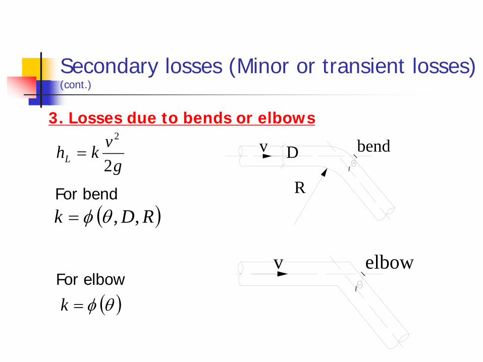
3. Losses due to bends or elbows
Secondary losses (Minor or transient losses) (cont.)
gvkhL 2
2
=
For bend( )RDk ,, θφ=
bendDv
R
v elbowFor elbow
( )θφ =k

4. Losses due to valves
Secondary losses (Minor or transient losses) (cont.)
gvkhL 2
2
=
plug valve butter fly valve gate valve

Loss
Coefficients

Bernoulli's Equation with Major and Minor Loss
LBB
AAA h
gV
DLfzP
gVzP
gV
++++=++222
222
γγB
54321 hhhhhhL ++++=
gVkh ii 2
2
=
Minor Loss Term
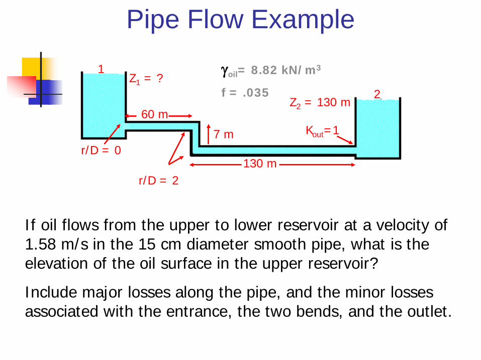
Pipe Flow Example
1
2Z2 = 130 m
130 m
7 m
60 m
r/D = 2
Z1 = ?γoil= 8.82 kN/m3
f = .035
If oil flows from the upper to lower reservoir at a velocity of 1.58 m/s in the 15 cm diameter smooth pipe, what is the elevation of the oil surface in the upper reservoir?
Include major losses along the pipe, and the minor losses associated with the entrance, the two bends, and the outlet.
Kout=1
r/D = 0

Pipe Flow Example
1
2Z2 = 130 m
130 m
7 m
60 m
r/D = 2
Z1 = ?
Kout=1
r/D = 0
Apply Bernoulli’s equation between points 1 and 2:Assumptions:
P1 = P2 = Atmospheric = 0 V1 = V2 = 0 (large tank)
0 + 0 + Z1 = 0 + 0 + 130m + Hmaj + Hmin
Hmaj = (f L V2)/(D 2g)=(.035 x 197m x (1.58m/s)2)/(.15 x 2 x 9.8m/s2)
Hmaj= 5.85m

Pipe Flow Example
1
2Z2 = 130 m
130 m
7 m
60 m
r/D = 2
Z1 = ?
Kout=1
r/D = 0
0 + 0 + Z1 = 0 + 0 + 130m + 5.85m + Hmin
Hmin= 2KbendV2/2g + KentV2/2g + KoutV2/2g
From Loss Coefficient table:
Kbend = 0.19 Kent = 0.5 Kout = 1
Hmin = (0.19x2 + 0.5 + 1) x (1.582/2x9.8)
Hmin = 0.24 m

Pipe Flow Example
1
2Z2 = 130 m
130 m
7 m
60 m
r/D = 2
Z1 = ?
Kout=1
r/D = 0
0 + 0 + Z1 = 0 + 0 + 130m + Hmaj + Hmin
0 + 0 + Z1 = 0 + 0 + 130m + 5.85m + 0.24m
Z1 = 136.1 m

Numerical Example: Minor LossConvert the piping system to an equivalent length of 6” pipe.

Numerical Example: Minor LossSolution
This problem will be solved by using the Bernoulli equation, A to M, datum M, as follows:
(0+0+h) = 0+0+0+(0.025x150/1+8.0+2x0.5+0.7+1.0)(V12
2/(2g)+(0.02x100/0.5+0.7+6.0+2x0.5+3.0+1.0)(V6
2/(2g)
)22
(2222
26
2
212
1
26
2
22
212
1
112
22
21
12
1
gVk
gVk
gV
DLf
gV
DLfzP
gVzP
gV
ici
ic∑ ++++++=++γγ
0 0 h 0 0 0
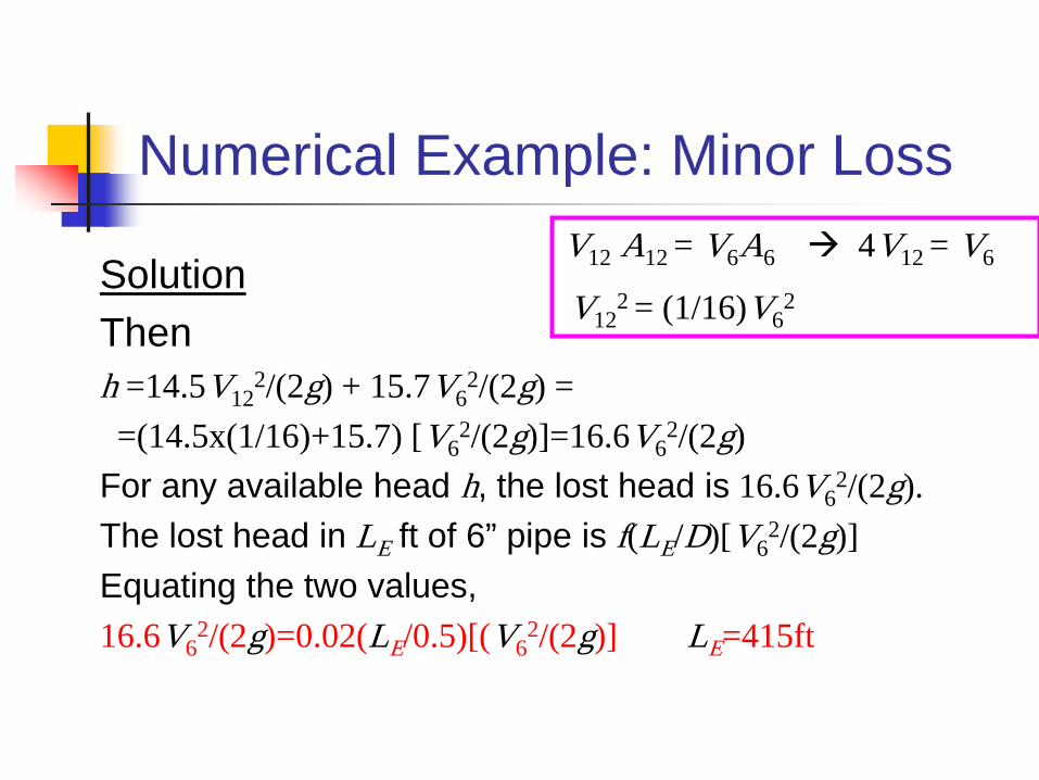
Numerical Example: Minor Loss
SolutionThenh =14.5V12
2/(2g) + 15.7V62/(2g) =
=(14.5x(1/16)+15.7) [V62/(2g)]=16.6V6
2/(2g)For any available head h, the lost head is 16.6V6
2/(2g).The lost head in LE ft of 6” pipe is f(LE/D)[V6
2/(2g)]Equating the two values,16.6V6
2/(2g)=0.02(LE/0.5)[(V62/(2g)] LE=415ft
V12 A12 = V6A6 4V12 = V6
V122 = (1/16)V6
2

Design of Single Pipe Flow
Type I: Head loss problemGiven flow rate and pipe combinations, determine the total head loss in a system
Type II: Discharge problemGiven allowable total head loss and pipe combinations, determine the flow rate
Type III: Sizing problemGiven allowable total head loss and flow rate, determine the pipe diameter

Type I: Head loss problems
Given the pipe material, pipe geometry, and flow rate, find out how much friction loss we may encounter over the pipe.
Application: pumping station design.

Type I: Head loss Problem A 20-in-diameter galvanized iron pipe 2
miles long carries 4 cfs of water at 60oF. Find the friction loss using Moody diagram
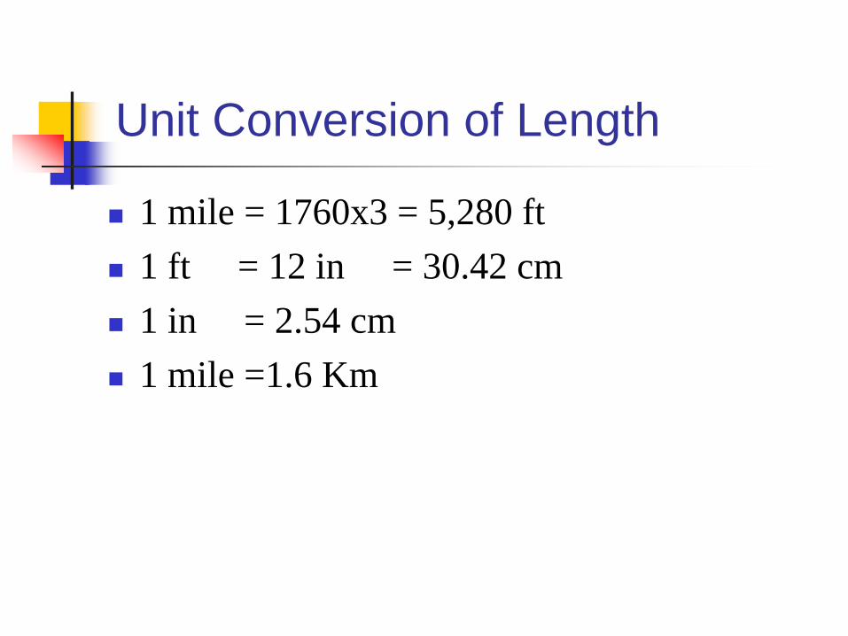
Unit Conversion of Length
1 mile = 1760x3 = 5,280 ft 1 ft = 12 in = 30.42 cm 1 in = 2.54 cm 1 mile =1.6 Km

Type I: Head loss Problem
e = 0.0005 ft, so e/D = 0.0005 (12)/20 = 0.0003L= 2 mile=2*(5280 ft/mile)= 10,560 ft
fpsDQV 8333.1
)12/20()4(44
22 ===ππ
for water at 60oF: ν = 1.217x10⁻⁵ ft2/sec
55 1051.2
10217.18333.1)12/20(
×=×
== −υDVRe
Turbulent flow
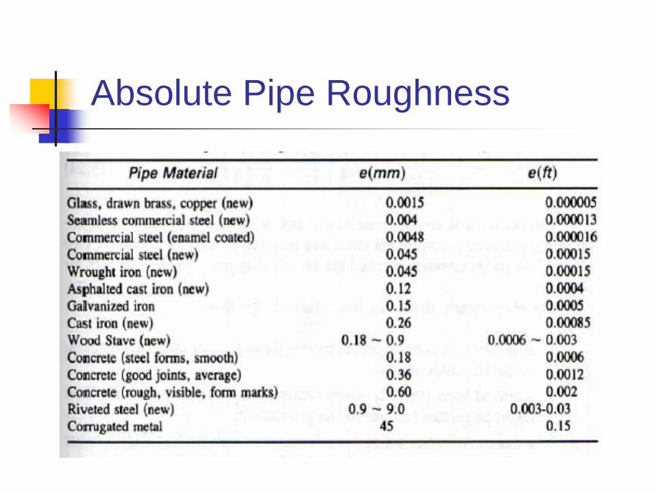
Absolute Pipe Roughness

Type I: Head loss Problem
Based on e/D and Re, we find our f = 0.0172 in the Moody Diagram, then we may obtain:
ftg
VDLfhf 69.5)
)2.32(28333.1)(
12/2010560(0172.0
2
22
===

Type II: Discharge Problem
Given the pipe material and friction loss gradient, find out how much fluid we may send over the pipe.
Application: leak detection.

Type II: Discharge Problem
Water at 20oC flows in a 500-mm diameter welded steel pipe.
If the friction loss gradient is 0.006, determine the flow rate.

Type II: Discharge Problem
For welded steel pipe:e = 0.046 mm; e/D =0.046/500 = 0.000092
At 20oC, = 1.003x10⁻⁶ m2/sec hf /L = 0.006 is given
2/1
2
2
243.081.9)2(5.0
006.0
21
fV
fVg
VD
fLh
S f
=
=
==
υ

Dimensional Analysis of Pipe FlowMoody Chart
Laminar
Marks Reynolds Number independence
Dimensional Analysis of Pipe FlowMoody Chart

Absolute Pipe Roughness

Type II: Discharge Problem For e/D = 0.000092 fmin~0.0118 (Moody Diagram) Try f = 0.0118 then V = 0.243/(0.0118)0.5 = 2.23 m/sec
With e/D =0.000092 and Re=1.114x10⁶; we may get f = 0.0131
Try one more time and show this results have converged
Q = AV = 0.416 m3/sec
66 10114.1
10003.1)23.2)(5.0(
×=×
== −υVDRe

Type III: Sizing Problem
Given the boundary condition of water head in the pipe system and the allowable head loss, determine the pipe diameter.
Application: designing the pipe system between the reservoir and the end user.

Type III: Sizing Problem
The allowable head loss is 5 m/km of pipe length.
Estimate the size of a uniform, horizontal welded-steel pipe installed to carry 500 l/sec of water at 10oC.

Type III: Sizing ProblemSolution Bernoulli’s equation can be applied to pipe
section 1 km apart
For a uniform, horizontal pipe with no localized head losses
V1=V2 z1 = z2
LB
BB
AAA h
gV
DLfzP
gVzP
gV
++++=++222
222
γγB

Type III: Sizing Problem
The Bernoulli’s equation reduces to
52
2
22
22 8)4/(22 Dg
fLQDgQ
DLf
gV
DLfhf ππ
===
fgfLQD 13.4
58
2
25 ==
π
(per each Km)mhPPf
BA 5==−γγ

Type III: Sizing Problem
Therefore L = 1000m, and hf = 5m. At 10oC, v =1.31x10⁻⁶ m2/sec. Assuming welded-steel roughness to be in
the lower range of riveted steel, e = 0.9 mm. Apply try and error procedure:
Assume D = 0.8 m
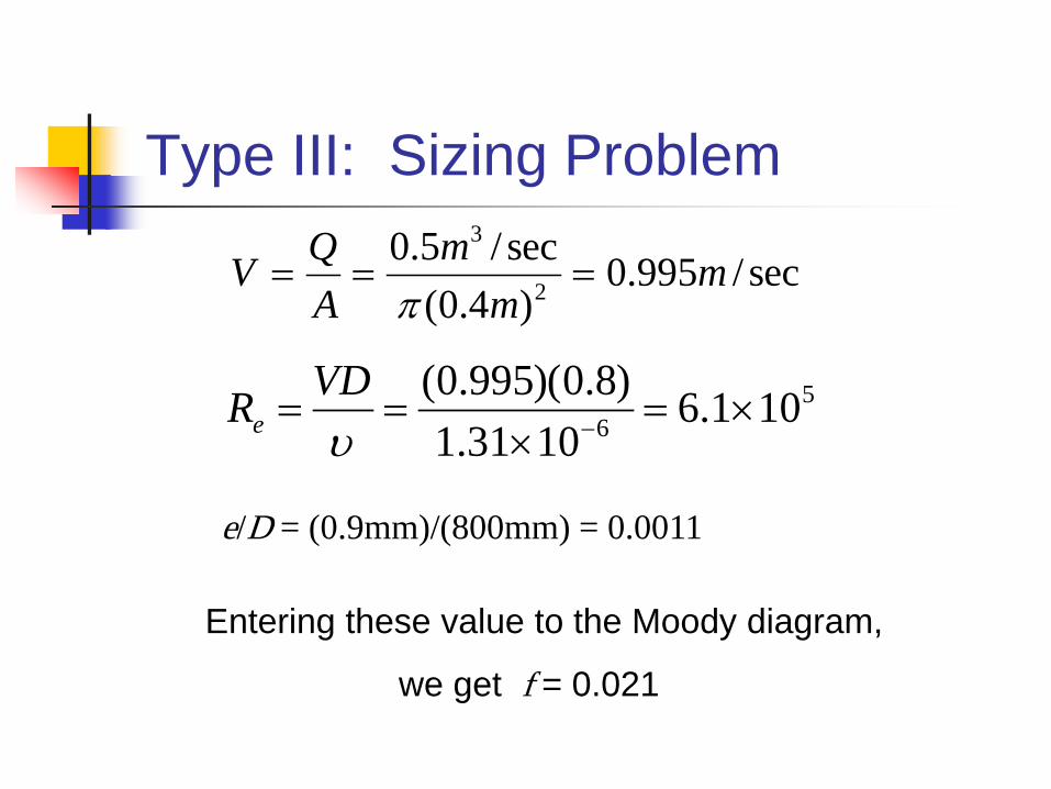
Type III: Sizing Problem
sec/995.0)4.0(
sec/5.02
3
mm
mAQV ===
π
e/D = (0.9mm)/(800mm) = 0.0011
Entering these value to the Moody diagram,
we get f = 0.021
56 101.6
1031.1)8.0)(995.0(
×=×
== −υVDRe
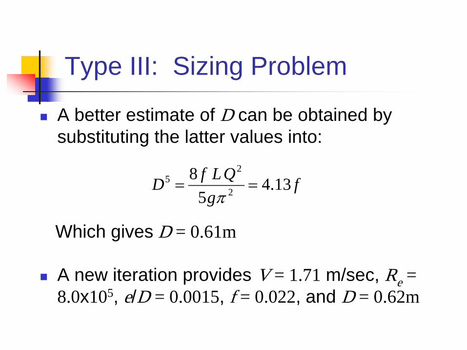
Type III: Sizing Problem
A better estimate of D can be obtained by substituting the latter values into:
A new iteration provides V = 1.71 m/sec, Re = 8.0x10⁵, e/D = 0.0015, f = 0.022, and D = 0.62m
fg
QLfD 13.45
82
25 ==
π
Which gives D = 0.61m

Software Applications
http://www.eng-software.com/