pipe flow 03

Linearized pipe flow to Reynolds number 107

�AA. Meseguer, L.N. Trefethen *

Computing Laboratory, Oxford University, Wolfson Building, Parks Road, Oxford OX1 3QD, UK

Received 4 May 2002; accepted 16 January 2003

Abstract

A Fourier–Chebyshev Petrov–Galerkin spectral method is described for high-accuracy computation of linearized

dynamics for flow in an infinite circular pipe. Our code is unusual in being based on solenoidal velocity variables and in

being written in MATLAB. Systematic studies are presented of the dependence of eigenvalues, transient growth factors,

and other quantities on the axial and azimuthal wave numbers and the Reynolds number R for R ranging from 102 to

the idealized (physically unrealizable) value 107. Implications for transition to turbulence are considered in the light of

recent theoretical results of S.J. Chapman.

� 2003 Elsevier Science B.V. All rights reserved.

1. Introduction

Three classical incompressible shear flows have received attention in connection with the phenomenon of

‘‘subcritical’’ or ‘‘nonmodal’’ or ‘‘bypass’’ transition to turbulence [9,28]. Plane Poiseuille and plane Couettechannel flows are the most accessible to theoretical analysis and numerical computation and have been the

subject of numerous studies [4,6,12,14,17,23,24,31]. Pipe flow (also known as pipe Poiseuille or Hagen–

Poiseuille flow) is the most accessible to laboratory experiments [7,8,35]. It was in the context of flow in a pipe

that Reynolds in 1883 identified the basic problem of this field: when and how do high-speed flows undergo

transition from the laminar state to more complicated states such as puffs, slugs, and turbulence [26]?

The present paper concerns the numerical simulation of pipe flow. It is a product of an ongoing col-

laboration between ourselves, working on the computer, and Prof. Tom Mullin of the University of

Manchester, working in the laboratory. A general aim of this collaboration is, by developing numerical andexperimental methods in tandem, to help narrow the gap between two communities and literatures that

have not communicated as well as they might have. Specifically, we aim to focus on some of the principal

mechanisms by which small perturbations in high speed flow may grow as they flow downstream and

develop into complicated structures associated with turbulence. Our focus is on the elucidation of key

mechanisms involved in transition, not on fully developed turbulence.

Journal of Computational Physics 186 (2003) 178–197

www.elsevier.com/locate/jcp

*Corresponding author. Tel.: +44-1865-273-886; fax: +44-1865-273-839.

E-mail address: [email protected] (L.N. Trefethen).

0021-9991/03/$ - see front matter � 2003 Elsevier Science B.V. All rights reserved.

doi:10.1016/S0021-9991(03)00029-9

mail to: [email protected]

With these aims in mind, and with an acute awareness of the continuing advance of desktop and laptop

computers, we have written a high accuracy Petrov–Galerkin spectral code for pipe flow in MATLAB. In

principle we are thus engaged in direct numerical simulation (DNS) of the Navier–Stokes equations. On the

computers available today, fully resolved DNS demands multiple processors, and MATLAB is not com-

petitive with Fortran or C for such computations. On a single processor, however, a well-designed

MATLAB code may run slower than the equivalent Fortran or C code by only a modest factor equivalent

to, say, a year or two of technological advance in hardware. In exchange for this modest cost in machine

speed one gets a great gain in human efficiency, flexibility, and compactness and portability of code, sinceMATLAB is a high-level language with the principal operations of linear algebra and fast Fourier trans-

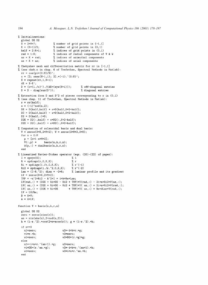
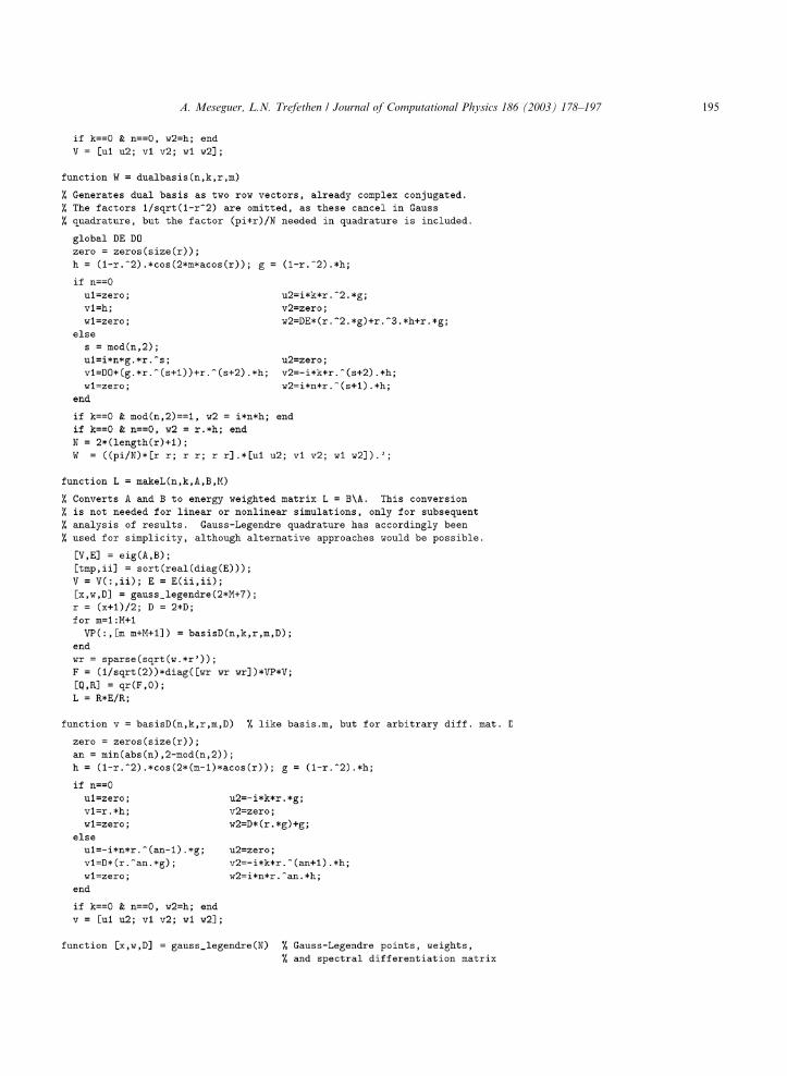
form built in, as well as powerful graphics. For example, our linearized pipe flow code is listed as a brief

appendix to this paper; one would hardly do such a thing with Fortran or C. Today, MATLAB is a good

vehicle for coarsely resolved pipe flows. In a few years, it will be good for medium resolution too.

This paper is devoted to linear effects, with nonlinear interactions deferred to a subsequent publication.

One reason for this is that the main features of our methods of discretization, which are not standard, can

be described in the linear context. Another is that in view especially of a recent paper of Chapman [6],

certain questions related to the nonlinear problem of transition to turbulence can be examined in the linearcase. In this paper we first describe our discretization, then present various numerical results that go beyond

those reported previously, including asymptotic expressions for various quantities as R ! 1. At the end we

consider some implications in the light of Chapman�s analysis.Previous numerical simulations of (nonlinear) pipe flow have included works of Boberg and Brosa [3],

Komminaho and Johansson [13], O�Sullivan and Breuer [21], Priymak and Miyazaki [22], Shan et al. [29],

Zhang et al. [36], and Zikanov [37]. In addition, various previous authors have simulated linearized pipe flow

[2,16,27,32]. Our methods could be summarized as a solenoidal scheme for the pipe of the sort proposed by

Leonard and Wray [16], but using Chebyshev rather than Jacobi polynomials, so that the FFT is applicable,which entails a Petrov–Galerkin rather than Galerkin formulation, as described by Moser et al. for other

geometries [20] (see also Section 7.3.3 of [5]); andwith regularity conditions at the center of the pipe imposed in

the manner of Priymak and Miyazaki [22,33]. Some further details of our work can be found in [18].

2. Pipe flow equations and laminar flow solution

In an infinite circular pipe of radius a, we consider the flow of an incompressible Newtonian fluidwith dynamic viscosity l and density q driven by an external constant axial pressure gradient

dp0=dz ¼ �P. Let V ¼ V ðtÞ denote the three-dimensional velocity field vector at a given time t; we use

the symbol V rather than the more usual v to make a distinction that can be carried over to the

computer program from the three components u, v, w to be introduced below. The Navier–Stokes

equations are

Vt þ ðV � rÞV ¼ q�1ðPzz�rp þ lDV Þ; ð1Þ

where the subscript denotes a partial derivative, zz is the unit vector in the axial direction, and p is the

pressure relative to p0; we supplement (1) with the zero-divergence equation

r � V ¼ 0 ð2Þ

and the no-slip condition V ¼ 0 on the boundary. The dimensions of each term in (1) are ðlengthÞ=ðtimeÞ2.We nondimensionalize by selecting space, time, and mass scales ½L� ¼ a, ½T � ¼ 4l=Pa, and ½M � ¼ qa3, re-spectively, and redefining accordingly the space and time variables and the dependent variables V and p.

A. Meseguer, L.N. Trefethen / Journal of Computational Physics 186 (2003) 178–197 179

Eq. (1) becomes

½L�½T �2

Vt þ½L�½T �2

ðV � rÞV ¼ q�1Pzz� q�1 ½M �½L�2½T �2

rp þ q�1l½T �½L�DV ;

or, after multiplying through by ½T �2=½L�,

Vt þ ðV � rÞV ¼ ½T �2

½L� q�1Pzz� q�1 ½M �½L�3

rp þ q�1l½T �½L�2

DV ;

which simplifies to

Vt þ ðV � rÞV ¼ 16l2

Pa3qzz�rp þ 4l2

Pa3qDV :

If we define the nondimensional Reynolds number by

R ¼ Pa3q4l2

; ð3Þ

then the equation becomes

Vt þ ðV � rÞV ¼ 4R�1zz�rp þ R�1DV : ð4Þ

These are the nondimensional Navier–Stokes equations for flow in a pipe.

We can express (4) explicitly in terms of cylindrical coordinates r (radial), h (azimuthal), and z (axial). If u, v,and w denote the radial, azimuthal, and axial components of V, respectively, then (4) takes the form [15]

ut þ uur þ r�1vuh þ wuz � r�1v2 ¼ �pr þ R�1ðurr þ r�1ur þ r�2uhh þ uzz � 2r�2vh � r�2uÞ; ð5Þ

vt þ uvr þ r�1vvh þ wvz þ r�1uv ¼ �r�1ph þ R�1ðvrr þ r�1vr þ r�2vhh þ vzz þ 2r�2uh � r�2vÞ; ð6Þ

wt þ uwr þ r�1vwh þ wwz ¼ 4R�1 � pz þ R�1ðwrr ¼ r�1wr þ r�2whh þ wzzÞ; ð7Þ

and Eq. (2) in cylindrical coordinates is

ur þ r�1vh þ wz þ r�1u ¼ 0: ð8Þ

The boundary condition now takes the form

u ¼ v ¼ w ¼ 0 for r ¼ 1: ð9Þ

It is readily seen that independently of R, there is a steady solution to (5)–(9), the laminar flow, consisting of

pure axisymmetric axial motion:

p ¼ �Pzþ const:; u ¼ 0; v ¼ 0; w ¼ 1� r2: ð10Þ

Note that in our nondimensional variables, the laminar flow has speed 1 at the centerline; this was the reason

for including the factor 4 in the definition of ½T �. In other words, an equivalent definition to (3) would be

R ¼ aqlUCL;

where UCL ¼ ½L�=½T � ¼ Pa2=4l is the velocity of the laminar flow at the centerline in dimensional units.

180 A. Meseguer, L.N. Trefethen / Journal of Computational Physics 186 (2003) 178–197

3. Linearization and reduction to Fourier modes

For numerical solution of the Navier–Stokes equations, it is convenient to take as dependent variables

the perturbation of the velocity field from the laminar solution. The result are equations in which the

velocity components interact both linearly and quadratically.

Our concern in this paper is the linearized problem in which only infinitesimal perturbations from the

laminar flow are considered. This is achieved by setting quadratic terms with respect to such perturbations

to zero. Let �pp ¼ const., �uu ¼ 0, �vv ¼ 0, and �ww ¼ 1� r2 denote the pressure and velocity variables of (10). Letp, u, v, and w denote the perturbations of these quantities from their laminar values. Then the linearizations

of (5)–(7) take the form

ut þ �wwuz ¼ �pr þ R�1ðurr þ r�1ur þ r�2uhh þ uzz � 2r�2vh � r�2uÞ; ð11Þ

vt þ �wwvz ¼ �r�1ph þ R�1ðvrr þ r�1vr þ r�2vhh þ vzz þ 2r�2uh � r�2vÞ; ð12Þ

wt þ u�wwr þ �wwwz ¼ �pz þ R�1ðwrr þ r�1wr þ r�2whh þ wzzÞ; ð13Þand (8) looks the same as before,

ur þ r�1vh þ wz þ r�1u ¼ 0: ð14Þ

Eqs. (11)–(14) are linear, and the cylindrical domain is periodic in h and unbounded in z. It follows that allsolutions to these equations can be expressed as superpositions of complex Fourier modes of the form

V ðr; h; z; tÞ ¼ eiðnhþkzÞV ðr; tÞ; pðr; h; z; tÞ ¼ eiðnhþkzÞpðr; tÞ ð15Þ

for appropriate functions V ðr; tÞ and pðr; tÞ, where n 2 Z and k 2 R. Moreover, the functions correspondingto different k or n are orthogonal, so there are no pitfalls in making use of such a decomposition. Let the r,

h, and z components of V ðr; tÞ be denoted by uðr; tÞ, vðr; tÞ, wðr; tÞ, respectively. Introducing (15) into (11)–

(13) gives the equations

ut ¼ �pr þ R�1ðurr þ r�1ur � n2r�2u� k2u� 2inr�2v� r�2uÞ � ik �wwu; ð16Þ

vt ¼ �r�1ph þ R�1ðvrr þ r�1vr � n2r�2v� k2vþ 2inr�2u� r�2vÞ � ik �wwv; ð17Þ

wt ¼ �pz þ R�1ðwrr þ r�1wr � n2r�2w� k2wÞ � u�wwr � ik �www ð18Þ

and (14) becomes

ur þ inr�1vþ ikwþ r�1u ¼ 0: ð19Þ

4. Solenoidal Petrov–Galerkin discretization

The numerical method we have chosen for (16)–(19) is adapted from work in the early 1980s by Leonard

and Wray [16] and Moser et al. [20]; see Section 7.3.3 of [5] for a summary. If (16)–(18) are a system of

linear partial differential equations of the form Vt ¼ LV , then the weak form of the same system is

ðVt ;W Þ ¼ ðLV ;W Þ for all W in a suitable space of test functions, where ð�; �Þ denotes the inner product overthe spatial domain. In our problem, because of (19), V is solenoidal (i.e., divergence-free) and zero at the

boundary. It follows that one may restrict attention to test functions W with the same properties, since if


ðV1;W Þ ¼ ðV2;W Þ for all solenoidal functions W that are zero at the boundary, then in particular

ðV1; V1 � V2Þ ¼ ðV2; V1 � V2Þ, i.e., ðV1 � V2; V1 � V2Þ ¼ 0, implying V1 ¼ V2. Now by (2.4), the terms involving

the pressure in ðLV ;W Þ are of the form ðrp;W Þ. Since W ¼ 0 at the boundary, integration by parts implies

that this is the same as �ðp;r � W Þ, which is zero since r � W ¼ 0. Thus by restricting attention to sole-

noidal velocity fields we have eliminated the pressure variable and the incompressibility condition (19) and

reduced (16)–(19) to the weak form

ðVt ;W Þ ¼ ðLV ;W Þ 8W ;

with LV defined by its three components

ðLV Þ1 ¼ R�1ðurr þ r�1ur � n2r�2u� k2u� 2inr�2v� r�2uÞ � ik �wwu; ð20Þ

ðLV Þ2 ¼ R�1ðvrr þ r�1vr � n2r�2v� k2vþ 2inr�2u� r�2vÞ � ik �wwv; ð21Þ

ðLV Þ3 ¼ R�1ðwrr þ r�1wr � n2r�2w� k2wÞ � u�wwr � ik �www: ð22Þ

For our numerical method, we will approximate V and W in finite-dimensional spaces of solenoidal

functions. This would be difficult in arbitrary geometries, but is feasible in the simple geometry of a pipe. In

what follows, we define

hmðrÞ ¼ ðl� r2ÞT2mðrÞ; gmðrÞ ¼ ð1� r2Þ2T2mðrÞ; ð23Þ

where T2m is the Chebyshev polynomial of degree 2m. We begin with V, distinguishing two cases depending

on whether n is zero or nonzero.

Case n ¼ 0. If n ¼ 0, the solenoidal condition (19) becomes ur þ r�1uþ ikw ¼ 0, implying that v is ar-

bitrary but u and w are related by a condition that we may write as

Dþuþ ikw ¼ 0;

where Dþ is an abbreviation for d=dr þ r�1. In addition, continuity of the velocity field at r ¼ 0 implies that

u (radial) and v (azimuthal) must be zero there, whereas w (axial) can be nonzero. Likewise, by (19), the no-

slip conditions imply ur at r ¼ 1. A suitable basis for functions satisfying these conditions is the set of

functions

V ð1Þm ¼

0rhmðrÞ0

0@

1A; V ð2Þ

m ¼�ikrgmðrÞ

0

Dþ½rgmðrÞ�

0@

1A ð24Þ

for m ¼ 0; 1; . . . ; except that if k ¼ 0, the third component of V ð2Þm is replaced by hmðrÞ.

Case n 6¼ 0. Here we take

V ð1Þm ¼

�inrjnj�1gmðrÞD½rjnjgmðrÞ�

0

0@

1A; V ð2Þ

m ¼0

�ikrjnjþ1hmðrÞinrjnjhmðrÞ

0@

1A: ð25Þ

Mathematically speaking, the factors of i in V ð2Þm could be dispensed with, but we leave them in so that the

basis functions have a desirable symmetry property: if k and n are negated, each basis function is replacedby its complex conjugate.


So much for the bases for the functions V. For the functionsW, we could take the same bases. However,

the resulting matrices would be dense, whereas they can be made to be banded if we choose W ð1Þm and W ð2Þ

m

instead as follows:

Case n ¼ 0.

W ð1Þm ¼ 1ffiffiffiffiffiffiffiffiffiffiffiffi

1� r2p

0hmðrÞ0

0@

1A; ð26Þ


1� r2p

ikr2gmðrÞ0

Dþ½r2gmðrÞ� þ r3hmðrÞ

0@

1A; ð27Þ

except that if k ¼ 0, the third component of W ð2Þm is replaced by rhmðrÞ.

Case n 6¼ 0. Define s ¼ 0 if n is even; 1 if n is odd. The basis functions are


1� r2p

inrsgmðrÞD½r1þsgmðrÞ� þ r2þshmðrÞ

0

0@

1A; ð28Þ


1� r2p

0

�ikr2þshmðrÞinr1þshmðrÞrg

0@

1A; ð29Þ

except that if k ¼ 0 and n is odd, the third component of W ð2Þm is replaced by inhmðrÞ.

For further details about (25)–(29). and for more comprehensive information about our numerical

method, including the analysis of regularity of solutions at the coordinate singularity r ¼ 0, see [18]. Alsosee Appendix A, which lists the code used to compute all the numerical results below.

5. Eigenvalues

We now begin to summarize some of the results of our computations. In doing this we have several

purposes. One is to record detailed enough results for assessment of the efficiency of our methods and for

future comparison by others. A second is to report various asymptotic expressions for behavior as R ! 1that have not been investigated before. A third is to review some of the main physical phenomena of

linearized pipe flow, which in combination with quadratic nonlinear couplings generate turbulence and

other flow effects. We shall see that even this purely linear analysis has implications for transition.

For much of the discussion we focus on two pairs of Fourier parameters:

n ¼ 1; k ¼ 0 and n ¼ 1; k ¼ 1: ð30Þ

Of course, many more wave numbers than these combine to make up an actual flow. These two choices,

nevertheless, represent two of the most important components of pipe flow dynamics: streamwise-inde-

pendent or more briefly just ‘‘streamwise’’ structures ðk ¼ 0Þ, with space and time scales OðRÞ, andstreamwise-dependent structures ðk 6¼ 0Þ, with space and time scales OðR1=2Þ or OðR1=3Þ. We remind thereader that although n is necessarily an integer, k can be any real number and has just been chosen to be an

integer for simplicity.

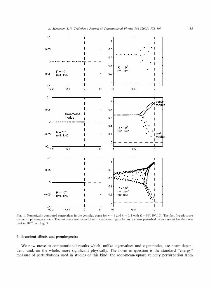
We begin with eigenvalues. Fig. 1 shows some of the rightmost eigenvalues in the complex plane of the

evolution operator L for the parameters (30) with R ¼ 103, 104, and 105. The values of M used were 8, 24,

74 for k ¼ 0 and 18, 57, 180 for k ¼ 1 for the three Reynolds numbers: the corresponding complex matrix


eigenvalue problems are of dimensions 18, 50, 150 and 38, 116, 362. We found these to be the minimum

values that give results converged to high accuracy, and each computation takes less than a second on our

workstation, except for the one with M ¼ 150.

Looking qualitatively at the figures, the first thing we note is that in the streamwise case k ¼ 0, all the

eigenvalues are real. They cluster close to the origin as R ! 1, revealing that certain streamwise modes are

only slightly damped for large R. For k ¼ 1, on the other hand, we have the three branches of eigenvalues

well known in pipe and channel flows and discussed, for example, in [9] and [28]. The eigenvalues k with

Imk � 0 correspond to wall modes, concentrated near the pipe wall and with low phase speed. The ei-genvalues k with Imk � 1 correspond to center modes, concentrated near the center of the pipe and with

phase speed close to 1. The remaining eigenvalues, extending in a line with Imk � 2=3 towards �1 in the

complex plane, correspond to global modes with phase speed � 2=3.For R ¼ 105, the expected line of eigenvalues with Imk � 2=3 does not appear in the last panel of Fig. 1:

instead we see a cloud of eigenvalues bounded by two cluster curves. These results are due to rounding errors,

and they do not improve ifM is increased.Mathematically speaking, they are incorrect, but this is a case where

the correct resultswouldbe nomoremeaningful physically than the incorrect ones, for aswe shall discuss in the

next section, the eigenvalues shown, and indeed all other numbers in the same general area of the complexplane, are exact eigenvalues of an operatorLþ DLwith kDLk < 10�10. In other words all of these numbers

are �-pseudo-eigenvalues ofL for a value of � far smaller the precision of any laboratory experiment.Table 1 lists the rightmost eigenvalues for the three cases of interest. We believe that these numbers

are correct in all but possibly the last of the 10 digits given. Fig. 2 shows details of convergence of the

rightmost center and wall eigenvalues for n ¼ 1 and k ¼ 1. (For k ¼ 0 the convergence is so fast that

M ¼ 5 suffices for 10-digit precision for all rightmost eigenvalues.) In verifying our code we have,

among other tests, compared certain numerical quantities against previously published results in [16]

and [22]. In [32] one can also find plots of eigenvalues in which results for the Fourier modes n and k

are not separated but superimposed in a single image; this corresponds to the spectrum of the whole

linear operator L rather than to various of its Fourier projections.

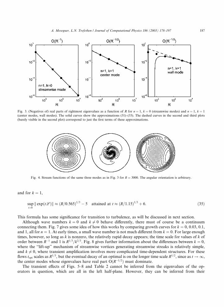
It is interesting to compare the asymptotic behavior of these three different kinds of eigenvalues, a

subject analyzed theoretically for channel flows (without numerical constants) in [6]. For the streamwise

case n ¼ 1 and k ¼ 0, the rightmost eigenvalue approaches 0 as R ! 1 almost exactly in proportion to R�1.

An approximation accurate to many digits is

kstreamwise � �14:6819706R�1: ð31ÞThe R�1 scaling implies that energy in this mode will decay on a time scale OðRÞ.

For n ¼ k ¼ 1, there are two eigenvalues of special interest. For the rightmost center mode eigenvalue, a

good approximation is

kcenter � i� ð2:28058þ 4:85519iÞR�1=2 þ ð0:92þ 0:32iÞR�1: ð32ÞThe imaginary part � 1 reflects the wave speed � 1, and the real part OðR�1=2Þ indicates decay on a time

scale OðR1=2Þ. For the rightmost wall mode eigenvalue, a good approximation is

kwall � ð�1:680þ 6:548iÞR�1=3 þ 14:3R�2=3 � 450iR�1: ð33Þ

Evidently these waves propagate with phase speed OðR1=3Þ and decay on a time scale OðR1=3Þ. This dif-ference between R�1=2 behavior for the center modes and R�1=3 behavior for the wall modes has been known

since work by Pekeris (1948), Corcos and Sellars (1959), and Gill (1965); see [9] for a summary and ref-

erences. These authors� analytical estimates concerned the axisymmetric case n ¼ 0; our estimates (32) and

(33) represent extensions to nonaxisymmetric flows.The approximations (31)–(33) are shown graphically in Fig. 3. Fig. 4 shows stream functions for these

three modes for R ¼ 3000.


6. Transient effects and pseudospectra

We now move to computational results which, unlike eigenvalues and eigenmodes, are norm-depen-

dent—and, on the whole, more significant physically. The norm in question is the standard ‘‘energy’’measure of perturbations used in studies of this kind, the root-mean-square velocity perturbation from

Fig. 1. Numerically computed eigenvalues in the complex plane for n ¼ 1 and k ¼ 0; 1 with R ¼ 103; 104; 105. The first five plots are

correct to plotting accuracy. The last one is not correct, but it is a correct figure for an operator perturbed by an amount less than one

part in 10�10; see Fig. 9.


laminar. Because the operators and matrices involved are nonnormal, this norm of a perturbation is not

simply proportional to the vector norm of its coefficients in an expansion in eigenvectors. Instead, to

calculate the norm correctly one must weight these coefficients by a nondiagonal matrix multiplication, as

discussed for example in Appendix A of [25]. We do not spell out the details, but they can be found in [18]

and are encoded in our MATLAB programs in Appendix A.

The most basic quantitative effect to look for is transient growth of three-dimensional ðn 6¼ 0Þ distur-bances, whose importance in shear flows was highlighted around 1990 by Boberg and Brosa [3], Butler and

Farrell [4], Gustavsson [12], and Reddy and Henningson [23], among others. Fig. 5 shows the maximum

possible transient growth as a function of t for various values of n with k ¼ 0 and k ¼ 1 (cf. Fig. 4 of [27],

Fig. 6 of [32], and Fig. 4 of [2]). In other words, it shows the operator norm k expðtLÞk as a function of t.

For the streamwise modes with k ¼ 0, the growth is substantial: amplification by a factor OðRÞ on a time

scale OðRÞ. For the nonstreamwise modes with k 6¼ 0, there is still a transient effect, but it is smaller:

amplification OðR1=3Þ on a time scale OðR1=3Þ. These exponents cannot be seen in Fig. 5, since just a single

value of R is shown, but they appear in Fig. 6, which displays the dependence on R on a log–log scale. Inthis figure and elsewhere, topt denotes the value of t at which k expðtLÞk is maximized.

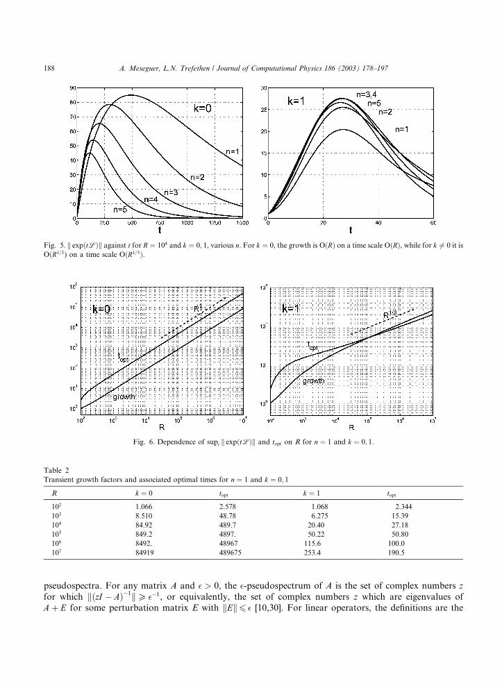
Table 2 lists the numbers underlying Fig. 6 for values of R equal to powers of 10. By analyzing these and

other such numbers we estimate for k ¼ 0,

supt<0

k expðtLÞk � R=117:7 attained at t � R=20:42; ð34Þ

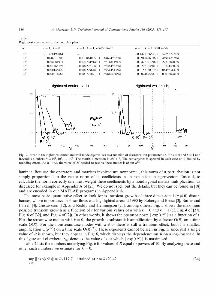
Table 1

Rightmost eigenvalues in the complex plane

R n ¼ 1; k ¼ 0 n ¼ 1; k ¼ 1, center mode n ¼ 1; k ¼ 1, wall mode

102 )0.1468197064 — )0.1471366653 + 0.5725629712i

103 )0.0146819706 )0.0708640053 + 0.8467498288i )0.0911426036 + 0.4691428789i

104 )0.0014681971 )0.0227049146 + 0.9514811947i )0.0472321996 + 0.2737887093i

105 )0.0001468197 )0.0072023080 + 0.9846498286i )0.0292364601 + 0.1372143077i

106 )0.0000146820 )0.0022796480 + 0.9951451356i )0.0153380019 + 0.0649631475i

107 )0.0000014682 )0.0007210913 + 0.9984646856i )0.0074895687 + 0.0303389812i

Fig. 2. Error in the rightmost center and wall mode eigenvalues as a function of discretization parameter M, for n ¼ 0 and k ¼ 1 and

Reynolds numbers R ¼ 102; 103; . . . ; 107. The matrix dimension is 2M þ 2, The convergence is spectral in each case until limited by

rounding errors. As R ! 1, the value of M needed to resolve these modes is about R1=3.


and for k ¼ 1,

supt>0

k expðtLÞk � ðR=0:565Þ1=3 � 5 attained at t � ðR=1:15Þ1=3 þ 6: ð35Þ

This formula has some significance for transition to turbulence, as will be discussed in next section.

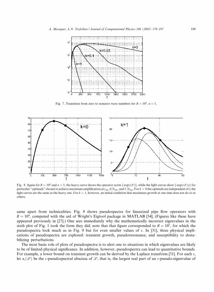
Although wave numbers k ¼ 0 and k 6¼ 0 behave differently, there must of course be a continuum

connecting them. Fig. 7 gives some idea of how this works by comparing growth curves for k ¼ 0, 0.03, 0.1,

and 1, all for n ¼ 1. At early times, a small wave number is not much different from k ¼ 0. For large enough

times, however, so long as k is nonzero, the relatively rapid decay appears; the time scale for values of k oforder between R�1 and 1 is R1=3=k2=3. Fig. 8 gives further information about the differences between k ¼ 0,

where the ‘‘lift-up’’ mechanism of streamwise vortices generating streamwise streaks is relatively simple,

and k 6¼ 0, where transient amplification involves more complicated time-dependent structures. For these

flows topt scales as R1=3, but the eventual decay of an optimal is on the longer time scale R1=2, since as t ! 1,

the center modes whose eigenvalues have real part OðR�1=2Þ must dominate.The transient effects of Figs. 5–8 and Table 2 cannot be inferred from the eigenvalues of the op-

erators in question, which are all in the left half-plane. However, they can be inferred from their

Fig. 3. (Negatives of) real parts of rightmost eigenvalues as a function of R for n ¼ 1, k ¼ 0 (streamwise modes) and n ¼ 1, k ¼ 1

(center modes, wall modes). The solid curves show the approximations (31)–(33). The dashed curves in the second and third plots

(barely visible in the second plot) correspond to just the first terms of these approximations.

Fig. 4. Stream functions of the same three modes as in Fig. 3 for R ¼ 3000. The angular orientation is arbitrary.


pseudospectra. For any matrix A and � > 0, the �-pseudospectrum of A is the set of complex numbers z

for which kðzI � AÞ�1kP ��1, or equivalently, the set of complex numbers z which are eigenvalues of

Aþ E for some perturbation matrix E with kEk6 � [10,30]. For linear operators, the definitions are the

Fig. 5. k expðtLÞk against t for R ¼ 104 and k ¼ 0; 1, various n. For k ¼ 0, the growth is OðRÞ on a time scale OðRÞ, while for k 6¼ 0 it is

OðR1=3) on a time scale OðR1=3Þ.

Fig. 6. Dependence of supt k expðtLÞk and topt on R for n ¼ 1 and k ¼ 0; 1.

Table 2

Transient growth factors and associated optimal times for n ¼ 1 and k ¼ 0; 1

R k ¼ 0 topt k ¼ 1 topt

102 1.066 2.578 1.068 2.344

103 8.510 48.78 6.275 15.39

104 84.92 489.7 20.40 27.18

105 849.2 4897. 50.22 50.80

106 8492. 48967 115.6 100.0

107 84919 489675 253.4 190.5


same apart from technicalities. Fig. 9 shows pseudospectra for linearized pipe flow operators with

R ¼ 104, computed with the aid of Wright�s Eigtool package in MATLAB [34], (Figures like these have

appeared previously in [27].) One sees immediately why the mathematically incorrect eigenvalues in the

sixth plot of Fig. 1 took the form they did; note that that figure corresponded to R ¼ 105, for which thepseudospectra look much as in Fig. 9 but for even smaller values of �. In [31], three physical impli-

cations of pseudospectra are explored: transient growth, pseudoresonance, and susceptibility to desta-

bilizing perturbations.

The most basic role of plots of pseudospectra is to alert one to situations in which eigenvalues are likely

to be of limited physical significance. In addition, however, pseudospectra can lead to quantitative bounds.

For example, a lower bound on transient growth can be derived by the Laplace transform [31]. For each �,let a�ðLÞ be the �-pseudospectral abscissa of L, that is, the largest real part of an �-pseudo-eigenvalue of

Fig. 7. Transition from zero to nonzero wave numbers for R ¼ 104, n ¼ 1.

Fig. 8. Again for R ¼ 104 and n ¼ 1, the heavy curve shows the operator norm k expðtLÞk, while the light curves show k expðtLÞvk forparticular ‘‘optimals’’ chosen to achievemaximumamplification at topt, 0:5topt, and 1:5topt. For k ¼ 0 the optimals are independent of t; thelight curves are the same as the heavy one. For k ¼ 1, however, an initial condition that maximizes growth at one time does not do so at

others.


L. From the Laplace transform it can be deduced that for some t; k expðtLÞk must be at least as large as�a�ðLÞ. Since this is true for each �, we can take the supremum to obtain

supt>0

k expðtLÞkP sup�>0

�a�ðLÞ: ð36Þ

For the pipe flow operator with k ¼ 0, n ¼ 1 we find

supt>0

k expðtLÞkPR=170:96; ð37Þ

a lower bound which is 69% of the true maximum of (34). The point zopt on the positive real axis corre-

sponding to the optimal � in (36) is zopt � ðR=20:11Þ�1.From (31) and (32) we know that the distance of the rightmost eigenvalue from the imaginary axis scales

for pipe flow with n ¼ 1 as R�1 for k ¼ 0 and R�1=2 for k ¼ 1. If these operators were normal, this would

imply that the maximum resolvent norm along the imaginary axis scaled like R1 and R1=2, respectively.

Infact, we find for k ¼ 0

supskðL� isIÞ�1k � ðR=28:89Þ2 þ ðR3=2Þ attained at s ¼ 0; ð38Þ

which is consistent with Eq. (7) of [32]. This number implies that the receptivity of pipe flow to external

disturbances at low frequency is of order OðR2Þ: a small vibration of the right form could induce a much

larger response.

7. Transition to turbulence

Transition to turbulence, like turbulence itself, depends on nonlinearity. Nevertheless, some insight

into the process can be obtained from the linearized problem. We shall make two observations in this

direction.

Fig. 9. Boundaries of �-pseudospectra of the linearized pipe flow operator for R ¼ 104, n ¼ 1, and k ¼ 0 and 1. From outside in, the

curves correspond to � ¼ 10�1, 10�2; . . . ; 10�10; only the first three are visible in the first figure. The second figure shows more striking

nonnormality: the eigenvalues at the center of the ‘‘Y’’ are so ill-conditioned as to be physically meaningless, a phenomenon first

identified for channel flows in [25]. It is the pseudospectra in the first figure that protrude more significantly into the right half-plane,

however, causing larger transient growth.


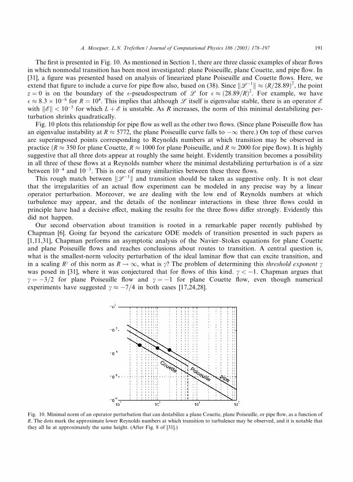
The first is presented in Fig. 10. As mentioned in Section 1, there are three classic examples of shear flows

in which nonmodal transition has been most investigated: plane Poiseuille, plane Couette, and pipe flow. In

[31], a figure was presented based on analysis of linearized plane Poiseuille and Couette flows. Here, we

extend that figure to include a curve for pipe flow also, based on (38). Since kL�1k � ðR=28:89Þ2, the pointz ¼ 0 is on the boundary of the �-pseudospectrum of L for � � ð28:89=RÞ2. For example, we have

� � 8:3� 10�6 for R ¼ 104. This implies that although L itself is eigenvalue stable, there is an operator Ewith kEk < 10�5 for which Lþ E is unstable. As R increases, the norm of this minimal destabilizing per-

turbation shrinks quadratically.Fig. 10 plots this relationship for pipe flow as well as the other two flows. (Since plane Poiseuille flow has

an eigenvalue instability at R � 5772, the plane Poiseuille curve falls to �1 there.) On top of these curves

are superimposed points corresponding to Reynolds numbers at which transition may be observed in

practice ðR � 350 for plane Couette, R � 1000 for plane Poiseuille, and R � 2000 for pipe flow). It is highly

suggestive that all three dots appear at roughly the same height. Evidently transition becomes a possibility

in all three of these flows at a Reynolds number where the minimal destabilizing perturbation is of a size

between 10�4 and 10�3. This is one of many similarities between these three flows.

This rough match between kL�1k and transition should be taken as suggestive only. It is not clearthat the irregularities of an actual flow experiment can be modeled in any precise way by a linear

operator perturbation. Moreover, we are dealing with the low end of Reynolds numbers at which

turbulence may appear, and the details of the nonlinear interactions in these three flows could in

principle have had a decisive effect, making the results for the three flows differ strongly. Evidently this

did not happen.

Our second observation about transition is rooted in a remarkable paper recently published by

Chapman [6]. Going far beyond the caricature ODE models of transition presented in such papers as

[1,11,31], Chapman performs an asymptotic analysis of the Navier–Stokes equations for plane Couetteand plane Poiseuille flows and reaches conclusions about routes to transition. A central question is,

what is the smallest-norm velocity perturbation of the ideal laminar flow that can excite transition, and

in a scaling Rc of this norm as R ! 1, what is c? The problem of determining this threshold exponent cwas posed in [31], where it was conjectured that for flows of this kind. c < �1. Chapman argues that

c ¼ �3=2 for plane Poiseuille flow and c ¼ �1 for plane Couette flow, even though numerical

experiments have suggested c � �7=4 in both cases [17,24,28].

Fig. 10. Minimal norm of an operator perturbation that can destabilize a plane Couette, plane Poiseuille, or pipe flow, as a function of

R. The dots mark the approximate lower Reynolds numbers at which transition to turbulence may be observed, and it is notable that

they all lie at approximately the same height. (After Fig. 8 of [31].)


Thus Chapman concludes that the exponent c observed in practice is different from the theoretically

correct value. Moreover, he puts forward an explanation for this discrepancy. Let us define

f ðRÞ ¼ log supt>0

k expðtLÞk� �

; ð39Þ

where L is the linearized Navier–Stokes operator for the given Reynolds number R and a fixed set ofnonzero Fourier parameters. The key point, Chapman argues, is that f ðRÞ curves downward as a function

of R. Because of this curvature, the slope of f ðRÞ for values of R in the ‘‘laboratory’’ range 103–104 is

greater than its asymptotic slope as R ! 1. Chapman shows how this single phenomenon feeds through

the various interactions to give an apparent c for physical or numerical experiments that is significantly

more negative than the true value.

Our computations for the pipe confirm Chapman�s observations for channels. The function f ðRÞappears in the second panel of Fig. 6, and it does indeed curve downward. The reason was encap-

sulated in (35),

supt>0

k expðtLÞk � ðR=0:565Þ1=3 � 5þOðR�1=3Þ: ð40Þ

This modest shift by about 5, entirely unremarkable from the general standpoint of asymptotics, can be

expected to make the apparent threshold exponent derived from pipe observations for R < 104 significantlydifferent from what would be found for R � 106. Chapman believes that the correct exponent is c ¼ �1 forpipe flow as for plane Couette flow (private communication), and nothing in our computations is incon-

sistent with that view.

8. Conclusion

In this paper we have proposed a new high-accuracy solenoidal Petrov–Galerkin spectral method forthe discretization of the linearized Navier–Stokes equations in an infinite circular pipe, with a MAT-

LAB implementation of this method given as a brief Appendix A. We have presented a range of

computational results that significantly extend what has been obtained before, focusing especially on

quantities related to nonmodal transient growth with azimuthal wave number n ¼ 1 and axial wave

numbers k ¼ 0 and k ¼ 1. These results go up to Reynolds number R ¼ 107, enabling us to obtain

asymptotic expressions as R ! 1 for a number of quantities including eigenvalue locations, transient

growth amplitude, transient growth time, and resolvent norms. Some of these asymptotic results are

summarized in Table 3. Similar tables of results for plane Couette and plane Poiseuille flows haveappeared in [31].

Although the results presented here are all linear, they shed light on the nonlinear problem of transition

to turbulence. In particular we find that the transient growth of nonstreamwise ðk 6¼ 0Þ modes approaches

Table 3

Summary of asymptotic results as R ! 1 (all attained with k ¼ 0, n ¼ 1)

Distance of spectrum from imag. axis ðR=14:68Þ�1kL�1k ðR=28:89Þ2supt>0 k expðtLÞk R=117:7topt for above R=20:42Lower bound based on pseudospectra R=171:0zopt for above ðR=20:11Þ�1


its R ! 1 asymptote slowly, as has been found by Chapman for channel flows [6], implying that one may

expect the apparent threshold exponent c for transition obtained from numerical or physical experiments in

the ‘‘laboratory’’ range of Reynolds numbers 103–104 to be more negative than its true asymptotic value as

R ! 1.

Our linear code has been extended to a fully nonlinear code for direct numerical solution of the Navier–

Stokes equations. For initial results from our nonlinear simulations, see [19].

Acknowledgements

This work was supported by UK EPSRC Grant GR/M30890. We have benefited from discussions with

Jon Chapman (Oxford University) and Tom Mullin (University of Manchester), including comments from

Chapman on a draft of this manuscript, and from advice over the years from Dan Henningson (Royal

Institute of Technology, Stockholm) and Peter Schmid (University of Washington).

Appendix A. MATLAB CODE


References

[1] J.S. Baggett, L.N. Trefethen, Low-dimensional models of subcritical transition to turbulence, Phys. Fluids 9 (1997) 1043.

[2] L. Bergstr€oom, Optimal growth of small disturbances in pipe Poiseuille flow, Phys. Fluids A 11 (1993) 2710.

[3] L. Boberg, U. Brosa, Onset of turbulence in a pipe, Z. Naturforsch. 43a (1988) 696.

[4] K.M. Butler, B.F. Farrell, Three-dimensional optimal perturbations in viscous shear flow, Phys. Fluids A 4 (1992) 1637.

[5] C. Canuto, M.Y. Hussaini, A. Quarteroni, T.A. Zang, Spectral Methods in Fluid Dynamics, Springer, New York, 1988.

[6] S.J. Chapman, Subcritical transition in channel flows, J. Fluid Mech. 451 (2002) 35.

[7] A.G. Darybyshire, T. Mullin, Transition to turbulence in constant mass-flux pipe flow, J. Fluid Mech. 289 (1995) 83.

[8] A.A. Draad, G.D.C. Kuiken, F.T.M. Nieuwstadt, Laminar-turbulent transition in pipe flow for Newtonian and non-Newtonian

fluids, J. Fluid Mech. 377 (1998) 267.

[9] P.G. Drazin, W.H. Reid, Hydrodynamic Stability, Cambridge University Press, Cambridge, 1981.

[10] M. Embree, L.N. Trefethen, Pseudospectra Gateway, web site at http://www.comlab.ox.ac.uk/pseudospectra.

[11] T. Gebhardt, S. Grossmann, Chaos transition despite linear stability, Phys. Rev. E 50 (1994) 3705.

[12] L.H. Gustavsson, Energy growth of three-dimensional disturbances in plane Poiseuille flow, J. Fluid Mech. 224 (1991) 241.

[13] J. Komminaho, A.V. Johansson, Development of a spectrally accurate DNS code for cylindrical geometries, part V of J.

Komminaho, Direct Numerical Simulation of Turbulent Flow in Plane and Cylindrical Geometries, Doctoral Thesis, Royal

Institute of Technology, Stockholm, 2000.

[14] G. Kreiss, A. Lundbladh, D.S. Henningson, Bounds for threshold amplitudes in subcritical shear flows, J. Fluid Mech. 270 (1994)

175.

[15] L.D. Landau, E.M. Lifshitz, Fluid Mechanics, Pergamon Press, Oxford, 1959.

[16] A. Leonard, A. Wray, A new numerical method for the simulation of three dimensional flow in a pipe, in: E. Krause (Ed.),

Proceedings of the 8th International Conference on Numerical Methods in Fluid Dynamics, Springer, Berlin, 1982.

[17] A. Lundbladh, D.S. Henningson, S.C. Reddy, Threshold amplitudes for transition in channel flows, in: Transition, Turbulence

and Combustion, vol. I, Kluwer Academic Publishers, Dordrecht, 1994.

[18] �AA. Meseguer and L.N. Trefethen, A spectral Petrov–Galerkin formulation for pipe flow I: linear stability and transient growth,

Rep. 00/18, Numerical Analysis Group, Oxford University, Computing Lab., 2000, available at http: //web.comlab.ox.ac.uk/oucl/

publications/natr/.

[19] �AA. Meseguer, L.N. Trefethen, A spectral Petrov–Galerkin formulation for pipe flow II: nonlinear transitional stages, Rep. 01/19,

Numerical Analysis Group, Oxford University, Computing Lab., 2001, available at http://web.comlab.ox.ac.uk/oucl/piiblications/

natr/.

[20] R.D. Moser, P. Moin, A. Leonard, A spectral numerical method for the Navier–Stokes equations with applications to Taylor–

Couette flow, J. Comp. Phys. 52 (1983) 524.

[21] P.L. O�Sullivan, K.S. Breuer, Transient growth in a circular pipe. I. Linear disturbances, Phys. Fluids 6 (1994) 3643.

[22] V.G. Priymak, T. Miyazaki, Accurate Navier–Stokes investigation of transitional and turbulent flows in a circular pipe, J. Comp.

Phys. 142 (1998) 370.

[23] S.C. Reddy, D.S. Henningson, Energy growth in viscous channel flows, J. Fluid Mech. 252 (1993) 209.

[24] S.C. Reddy, P.J. Schmid, J.S. Baggett, D.S. Henningson, On stability of streamwise streaks and transition thresholds in plane

channel flows, J. Fluid Mech. 365 (1998) 269.


http://www.comlab.ox.ac.uk/pseudospectra

http://http://web.comlab.ox.ac.uk/oucl/publications/natr/

http://http://web.comlab.ox.ac.uk/oucl/publications/natr/

http://web.comlab.ox.ac.uk/oucl/piiblications/natr/

http://web.comlab.ox.ac.uk/oucl/piiblications/natr/

[25] S.C. Reddy, P.J. Schmid, D.S. Henningson, Pseudospectra of the Orr–Sommerfeld operator, SIAM J. Appl. Math. 53 (1993) 15.

[26] O. Reynolds, An experimental investigation of the circumstances which determine whether the motion of water shall be direct or

sinuous, and of the law of resistance in parallel channels, Philos. Trans. Roy. Soc. 174 (1883) 935.

[27] P.J. Schmid, D.S. Henningson, Optimal energy growth in Hagen–Poiseuille flow, J. Fluid Mech. 277 (1994) 197.

[28] P.J. Schmid, D.S. Henningson, Stability and Transition in Shear Flows, Springer, New York, 2001.

[29] H. Shan, B. Ma, Z. Zhang, F.T.M. Nieuwstadt, Direct numerical simulation of a puff and a slug in transitional cylindrical pipe

flow, J. Fluid Mech. 387 (1999) 39.

[30] L.N. Trefethen, Pseudospectra of linear operators, SIAM Rev. 39 (1999) 247.

[31] L.N. Trefethen, A.E. Trefethen, S.C. Reddy, T.A. Driscoll, Hydrodynamic stability without eigenvalues, Science 261 (1993) 578.

[32] A.E. Trefethen, L.N. Trefethen, P.J. Schmid, Spectra and pseudospectra for pipe Poiseuille flow, Comp. Meth. Appl. Mech. Eng.

1926 (1999) 413.

[33] L.S. Tuckerman, Divergence-free velocity fields in nonperiodic geometries, J. Comp. Phys. 80 (1989) 403.

[34] T.G. Wright, Eigtool (MATLAB software package), available at http://www.comlab.ox.ac.uk/pseudospectra/eigtool/.

[35] I.J. Wygnanski, F.H. Champagne, On transition in a pipe. Part 1. The origin of puffs and slugs and the flow in a turbulent slug, J.

Fluid Mech. 59 (1973) 281.

[36] Y. Zhang, A. Gandhi, A.G. Tomboulides, S.A. Orszag, Simulation of pipe flow, in: Application of Direct and Large Eddy

Simulation to Transition and Turbulence, AGARD Conference, Crete, 1994, pp. 17.1–17.9.

[37] O.Yu. Zikanov, On the instability of pipe Poiseuille flow, Phys. Fluids 8 (1996) 2923.


http://www.comlab.ox.ac.uk/pseudospectra/eigtool/

pipe flow 03

Documents

numerical simulation

pipe poiseuille

linearized pipe

numerical computation

developed turbulence

innite circular pipe

reynolds number r

oxford university