This is an electronic reprint of the original article.This reprint may differ from the original in pagination and typographic detail.

Powered by TCPDF (www.tcpdf.org)

This material is protected by copyright and other intellectual property rights, and duplication or sale of all or part of any of the repository collections is not permitted, except that material may be duplicated by you for your research use or educational purposes in electronic or print form. You must obtain permission for any other use. Electronic or print copies may not be offered, whether for sale or otherwise to anyone who is not an authorised user.

Prepelita, Sebastian; Gomez Bolanos, Javier; Geronazzo, Michele; Mehra, Ravish; Savioja,LauriPinna-related transfer functions and lossless wave equation using finite-difference methods

Published in:Journal of the Acoustical Society of America

DOI:10.1121/1.5131245

Published: 01/11/2019

Document VersionPublisher's PDF, also known as Version of record

Published under the following license:CC BY

Please cite the original version:Prepelita, S., Gomez Bolanos, J., Geronazzo, M., Mehra, R., & Savioja, L. (2019). Pinna-related transferfunctions and lossless wave equation using finite-difference methods: Verification and asymptotic solution.Journal of the Acoustical Society of America, 146(5), 3629-3645. https://doi.org/10.1121/1.5131245

Pinna-related transfer functions and lossless wave equation using finite-differencemethods: Verification and asymptotic solutionSebastian T. PrepeliȚă, Javier Gómez Bolaños, Michele Geronazzo, Ravish Mehra, and Lauri Savioja

Citation: The Journal of the Acoustical Society of America 146, 3629 (2019); doi: 10.1121/1.5131245View online: https://doi.org/10.1121/1.5131245View Table of Contents: https://asa.scitation.org/toc/jas/146/5Published by the Acoustical Society of America

ARTICLES YOU MAY BE INTERESTED IN

Perception and preference of reverberation in small listening rooms for multi-loudspeaker reproductionThe Journal of the Acoustical Society of America 146, 3562 (2019); https://doi.org/10.1121/1.5135582

Octave stretching phenomenon with complex tones of orchestral instrumentsThe Journal of the Acoustical Society of America 146, 3203 (2019); https://doi.org/10.1121/1.5131244

Room acoustic modeling and auralization at an indoor firing rangeThe Journal of the Acoustical Society of America 146, 3868 (2019); https://doi.org/10.1121/1.5132286

Analytical and numerical methods for efficient calculation of edge diffraction by an arbitrary incident signalThe Journal of the Acoustical Society of America 146, 3577 (2019); https://doi.org/10.1121/1.5134065

Machine learning in acoustics: Theory and applicationsThe Journal of the Acoustical Society of America 146, 3590 (2019); https://doi.org/10.1121/1.5133944

Skewing of the glottal flow with respect to the glottal area measured in natural production of vowelsThe Journal of the Acoustical Society of America 146, 2501 (2019); https://doi.org/10.1121/1.5129121

Pinna-related transfer functions and lossless wave equationusing finite-difference methods: Verification and asymptoticsolution

Sebastian T. Prepelit�aa)

Department of Computer Science, Aalto University, Otaniementie 17, P.O. Box 15500, FI-00076 Aalto,Finland

Javier G�omez Bola~nosb)

Department of Signal Processing and Acoustics, Aalto University, P.O. Box 13000, FI-00076 Aalto Espoo,Finland

Michele GeronazzoDepartment of Architecture, Design, and Media Technology, Aalborg University, A. C. Meyers Vænge 15,2450 København SV, Denmark

Ravish MehraFacebook Reality Labs, 8747 Willows Road, Redmond, Washington 98052, USA

Lauri SaviojaDepartment of Computer Science, Aalto University, Otaniementie 17, P.O. Box 15500, FI-00076 Aalto,Finland

(Received 23 April 2019; revised 7 October 2019; accepted 10 October 2019; published online 27November 2019)

A common approach when employing discrete mathematical models is to assess the reliability and

credibility of the computation of interest through a process known as solution verification. Present-

day computed head-related transfer functions (HRTFs) seem to lack robust and reliable assessments

of the numerical errors embedded in the results which makes validation of wave-based models

difficult. This process requires a good understanding of the involved sources of error which are sys-

tematically reviewed here. The current work aims to quantify the pinna-related high-frequency

computational errors in the context of HRTFs and wave-based simulations with finite-difference

models. As a prerequisite for solution verification, code verification assesses the reliability of the

proposed implementation. In this paper, known and manufactured formal solutions are used and tai-

lored for the wave equation and frequency-independent boundary conditions inside a rectangular

room of uniform acoustic wall-impedance. Asymptotic estimates for pinna acoustics are predicted

in the frequency domain based on regression models and a convergence study on sub-millimeter

grids. Results show an increasing uncertainty with frequency and a significant frequency-dependent

change among computations on different grids. VC 2019 Author(s). All article content, except whereotherwise noted, is licensed under a Creative Commons Attribution (CC BY) license (http://creati-vecommons.org/licenses/by/4.0/). https://doi.org/10.1121/1.5131245

[FCS] Pages: 3629–3645

I. INTRODUCTION

The head-related transfer functions (HRTFs) represent

the acoustical paths from a stationary sound source to the

ears of the listener under free field conditions, encoding the

anatomical filtering effects which embed the auditory cues

used for localizing sound sources.

Unless cue remapping occurs,1 HRTFs are usually not

perceptually transferable.2 This is mainly due to the high

degree of personalization of the human pinna.3 Currently,

the main two methods for obtaining an estimate of individu-

alized HRTFs are measurements and simulations.

Measurements are the traditional method, based on which

HRTFs were perceptually validated.4–7 Although HRTF

measurements can nowadays be done within a relatively

short time,8–10 they are still, in many ways, impractical:

high accuracy could be challenging, specialized equipment

prevents scalability, while subjects undergo a generally

tedious measurement session.

Wave-based numerical simulations are an alternative

which could eventually offer greater flexibility when com-

pared to measurements. Presently, the boundary element

method (BEM)11–15 and the finite difference time domain

(FDTD)16–18 methods are the most common HRTF simula-

tion methods. Despite the many attractive properties of the

HRTF numerical simulations, their validity and reliability in

the full audible frequency bandwidth has not yet been estab-

lished using strong validation studies as those defined in the

verification and validation (V&V) literature.19,20 Moreover,

studies of numerical sensitivity/uncertainty analysis involv-

ing HRTF simulations are also scarce.18,21

a)Electronic mail: sebastian.prepelita@aalto.fib)Current address: Hefio Ltd., Otakaari 5 A, 02150 Espoo, Finland.

J. Acoust. Soc. Am. 146 (5), November 2019 VC Author(s) 2019. 36290001-4966/2019/146(5)/3629/17

The most challenging HRTF phenomena to be simulated

are the pinna effects which occur above 3 kHz.22 The pinna-

related transfer function (PRTF) provides the isolated infor-

mation of the pinna acoustics and can be used to focus the

analysis to such a challenging problem.

Any computation will contain approximations and spe-

cific errors which could render the result unreliable. Present

HRTF computations seem to lack a strong formal assessment

of reliability and credibility of the computed solutions.

Consequently, it not only becomes difficult to assess the pre-

dictive quality of the wave-based model employed, but also

wrong conclusions could be reached. The present study aims

to quantify the quality of computed wave-based PRTF/

HRTF solutions with focus on FDTD methods. Formal solu-

tions and their precision are estimated by asymptotically

extrapolating the results from computations on multiple sub-

millimeter grids. In turn, the uncertainty between HRTF

measurements and simulations can be quantified to the com-

plementary benefit of both approaches.23

This work is the first part of a comprehensive V&V

study. Validation with measurements of the present PRTF

results will be part of a separate validation study.

II. BACKGROUND

Linear acoustics is described by a linear and well-

posed continuous problem (in the Hadamard sense). Thus,

any consistent and stable approximation will theoretically

converge to the same solution (invoking the Lax-Richtmyer

equivalence theorem), independent of the mathematical

formulation of the continuous model and of the discrete

model employed (e.g., BEM, FDTD). Depending on the

formulation and properties of the continuous solution, any

computational implementation and execution will involve

model-specific deviations from the formal behavior. In

practice, such computational errors could interact in a com-

plex manner thus requiring empirical reliability assessment

of the final computations.

Here, a simple explicit and stable24 finite-difference

method is chosen which is amenable to parallelization. Its

simplicity and extensive study facilitates the understanding

of various error sources present in a final computation.

Moreover, the finite-difference literature is extensive and

offers formal methods/models to study the usually-dominant

(Ref. 20, p. 286) discretization error. Such methods can be

transferred from other fields and advantageously employed

to empirically estimate the quality of the computations,

given the complex PRTF problem at hand.

A. PRTFs

The PRTFs are formally defined in the frequency

domain as the following transfer function:

PRTFðr1;XÞ ¼Pearðr1;XÞPrefðr1;XÞ

; (1)

where r1 2 R3 denotes the continuous location of the

source, PearðXÞ represents the Fourier transform of the cap-

tured pressure at a fixed location of interest inside a pinna

cavity, and PrefðXÞ is the Fourier transform of a recorded

pressure with the pinna absent.

B. Continuous model

As partial differential equation (PDE), the inhomoge-

neous scalar wave equation (Ref. 25, p. 162) is considered

which can be written in some continuous three-dimensional

(3D) domain D as

@2pðr; tÞ@t2

¼ c2$2pðr; tÞ þ f ðr; tÞ; (2)

where r ¼ ½x; y; z�T 2 D (with D � R3), t represents time,

r ¼ ½ð@=@xÞ; ð@=@yÞ; ð@=@zÞ� represents the 3D Cartesian

del differential operator, c is the sound speed, p : R3 �Rþ! R is the scalar pressure field, and f : R3 �Rþ ! R is a

general analytical forcing or driving function. c is assumed

constant in the homogeneous and quiescent medium within D.

At the boundary surface(s) @D, the following frequency-

independent resistive boundary condition (BC) of local reaction

is employed for the pressure field:

�n � $pðrb; tÞ ¼bðrbÞ

c

@pðrb; tÞ@t

; (3)

where n represents the outward (pointing, locally, from Dinto any solid in contact with D) normal to the surface

boundary at point rb 2 @D, and b is the specific acoustic

admittance at the boundary (Ref. 26, p. 261), see the deriva-

tion in, e.g., the work by Kowalczyk and van Walstijn.27

C. Discrete models

In this study, an FDTD mathematical model is used to

discretize Eq. (2). Rigorously, the update discretizes the inte-

gral form of Eq. (2), however for the uniform Cartesian grid

used, the discretization of the strong form in Eq. (2) is

found24 for the interior update.

The second-order accurate standard rectilinear (SRL)

explicit update is obtained on the interior and employed on a

cubic Cartesian grid with voxel size of DX. A frequency inde-

pendent impedance can be set for the locally reacting stair-

cased boundaries using an “upwind” approximation for the

pressure field at the boundary.28 The code supports three types

of sources: soft, hard, and transparent.29 The explicit FDTD

update can be derived using finite volume (FV) methods24 and

can compactly be written for pressure and a soft source as

Pnþ1i 1þ NikC

bi

2

� �¼ k2

CX6�Ni

j¼1

Pnj � Pn

i

� �þ 2Pni

�Pn�1i 1� NikC

bi

2

� �þ DT2Fn

i ;

(4)

where Pi represents the discretized pressure field at the 3D

Cartesian index i, j indexes the neighboring air voxels for

Pi; kC ¼ cDT=DX is the Courant number (c is the sound

speed), Ni 2 f0; 1; 2;…; 6g represents the total number of solid

(i.e., boundary) voxels adjacent to Pi [for Ni¼ 6 the sum in Eq.

(4) is assumed to be 0], and Fi represents the local forcing

3630 J. Acoust. Soc. Am. 146 (5), November 2019 Prepelit�a et al.

applied at the center of voxel i. In Eq. (4), for computer mem-

ory considerations, a unique specific acoustic admittance bi is

assumed for all boundary surfaces of each voxel i.For simplicity and unambiguous definition of the grid spac-

ing DX, the boundaries are discretized on the same uniform 3D

Cartesian grid resulting in stair-stepped boundaries which are

obtained from the mesh by using a voxelization algorithm. The

adopted voxelization algorithm is the conservative30 one since,

although not ideal, it is well-defined and convenient to use.

1. Distributed computing model

The simulation domain was split against the Cartesian zaxis: D is partitioned in domains distributed across comput-

ing nodes, while each domain is partitioned in subdomainsacross Graphics Processing Unit (GPU) devices available at

each compute node. See more details about the implementa-

tion in Appendix B.

To avoid extra difficulties for a potential validation study

such as convergence rates and correspondence with reality, the

PRTF domain will be chosen without a commonly-employed

perfectly matched layer absorbing bounding boundary.

Consequently, the PRTF domain size is scaled such that no

reflection from the room walls arrives at the receiver locations.

D. Simulation errors

Depending on modeling and computational choices,

there are multiple sources of error,31 which could coexist in

a simulated result and affect the computations. Such errors

make it highly unlikely that the formal (i.e., asymptotic, as

DX ! 0) solution is computed in practice: given a discrete

model and its computational implementation, the discrete

solution will at best be within a ball Bðpðr; tÞ; eÞ of radius eproportional to the machine epsilon away from the unique

formal solution p(r,t). As such, it is useful to identify and

understand the behavior of the main sources of error for the

model and problem at hand, also considering that error can-

cellation could occur (Ref. 20, p. 382) in a computation

when multiple sources of error are present, together with

other unacknowledged23 errors.

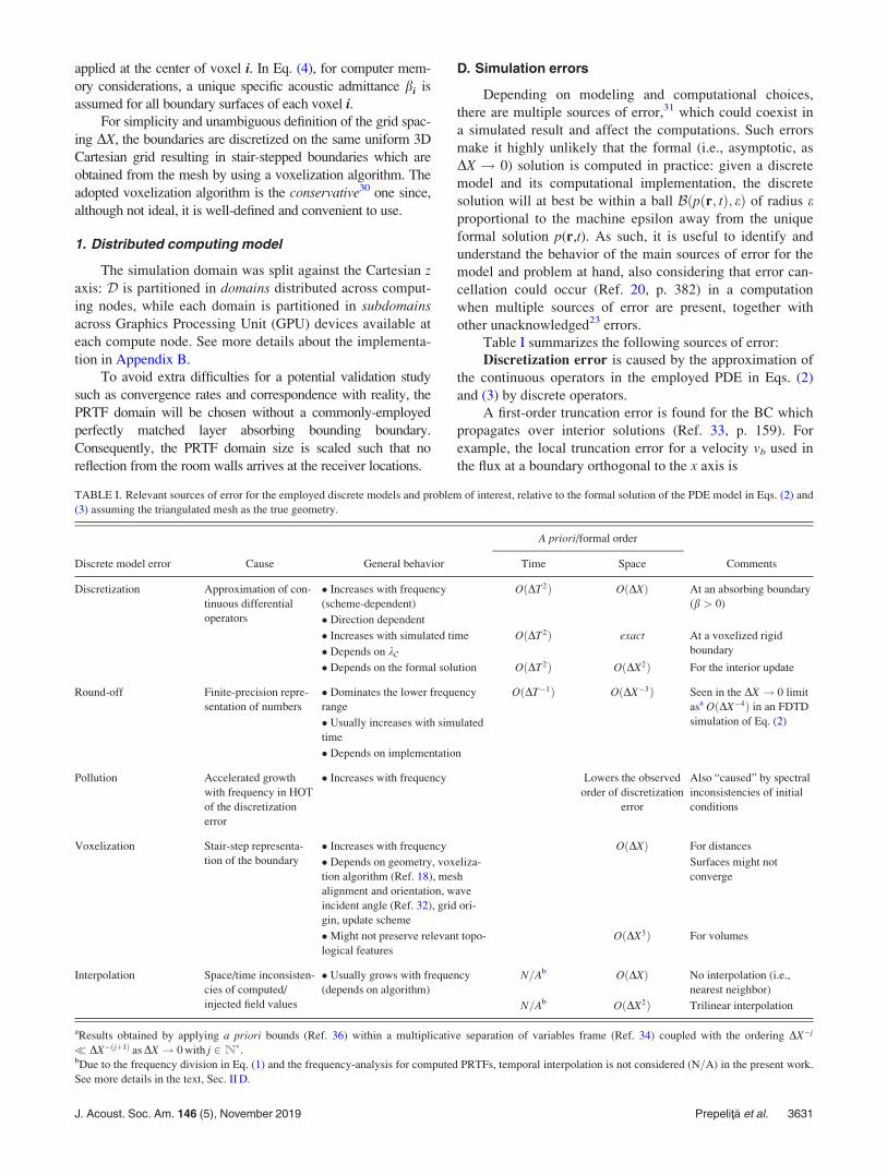
Table I summarizes the following sources of error:

Discretization error is caused by the approximation of

the continuous operators in the employed PDE in Eqs. (2)

and (3) by discrete operators.

A first-order truncation error is found for the BC which

propagates over interior solutions (Ref. 33, p. 159). For

example, the local truncation error for a velocity vb used in

the flux at a boundary orthogonal to the x axis is

TABLE I. Relevant sources of error for the employed discrete models and problem of interest, relative to the formal solution of the PDE model in Eqs. (2) and

(3) assuming the triangulated mesh as the true geometry.

A priori/formal order

Discrete model error Cause General behavior Time Space Comments

Discretization Approximation of con-

tinuous differential

operators

� Increases with frequency

(scheme-dependent)

OðDT2Þ OðDXÞ At an absorbing boundary

(b > 0)

� Direction dependent

� Increases with simulated time OðDT2Þ exact At a voxelized rigid

boundary� Depends on kC� Depends on the formal solution OðDT2Þ OðDX2Þ For the interior update

Round-off Finite-precision repre-

sentation of numbers

� Dominates the lower frequency

range

OðDT�1Þ OðDX�3Þ Seen in the DX ! 0 limit

asa OðDX�4Þ in an FDTD

simulation of Eq. (2)� Usually increases with simulated

time

� Depends on implementation

Pollution Accelerated growth

with frequency in HOT

of the discretization

error

� Increases with frequency Lowers the observed

order of discretization

error

Also “caused” by spectral

inconsistencies of initial

conditions

Voxelization Stair-step representa-

tion of the boundary

� Increases with frequency OðDXÞ For distances

� Depends on geometry, voxeliza-

tion algorithm (Ref. 18), mesh

alignment and orientation, wave

incident angle (Ref. 32), grid ori-

gin, update scheme

Surfaces might not

converge

�Might not preserve relevant topo-

logical features

OðDX3Þ For volumes

Interpolation Space/time inconsisten-

cies of computed/

injected field values

� Usually grows with frequency

(depends on algorithm)

N=Ab OðDXÞ No interpolation (i.e.,

nearest neighbor)

N=Ab OðDX2Þ Trilinear interpolation

aResults obtained by applying a priori bounds (Ref. 36) within a multiplicative separation of variables frame (Ref. 34) coupled with the ordering DX�j

� DX�ðjþ1Þ as DX! 0 with j 2N.bDue to the frequency division in Eq. (1) and the frequency-analysis for computed PRTFs, temporal interpolation is not considered (N=A) in the present work.

See more details in the text, Sec. II D.

J. Acoust. Soc. Am. 146 (5), November 2019 Prepelit�a et al. 3631

vbðtÞ � bbPjðtÞ ¼ bb

DX

2

@pbðtÞ@xþ bb � HOTðtÞ; (5)

where pb is the pressure at the boundary surface b, Pj is the

pressure at the center of a neighboring voxel j, bb is the spe-

cific acoustic admittance at b, and HOT stands for19 “higher

order terms” in DX.

Analysis of the global discretization error is generally

making use of a series expansion of the truncation error. For

the employed scheme and temporarily ignoring the initial

conditions and the boundary modeling, as DX,DT ! 0, an

FDTD-simulated pressure epr1ðtÞ at r ¼ r1 2 R3 can be

expressed as (Ref. 33, p. 217)

epr1ðt;DT;DXÞ ¼ pr1

ðtÞ þ �t;r1ðtÞDT2

þ �x;r1ðtÞDXq þ HOTðtÞ; (6)

where pr1ðtÞ is the asymptotic solution; �t;r1

ðtÞ and �x;r1ðtÞ are

the principal (Ref. 33, p. 158) temporal and spatial error terms,

respectively, q is the leading spatial formal accuracy which can

either be 2 for rigid boundaries or 1 for absorbing boundaries

close enough to r1; and HOT ¼ OðDT4;DX2qÞ. For fixed

r1; �t;r1ðtÞ satisfies a differential equation that depends on

the update and pr1ðtÞ (see, e.g., Secs. III 9 and III 10 in

Hairer et al.33) while the temporal dependence of �x;r1ðtÞ is

given by pr1ðtÞ.34 Thus, even a discrete delta sequence can be

used as the excitation signal without aliasing of the discrete-

time Fourier transform (DTFT) of the error terms Et=xðxÞ¼ DTFTf�t=xðtÞg and HOT(x) in Eq. (6).

Asymptotic range is attained when the deviation of the

discrete solution from the formal solution behaves according

to the expected leading19,35 space and/or time truncation

error terms. In the following, it is assumed the discrete solu-

tions are stepped at stable values of kC with negligible global

interactions (e.g., cancellation) between the spatial and tem-

poral truncation errors.

Round-off errors emerge due to the finite precision repre-

sentation of numbers in the FDTD solver. A priori analysis

shows divergence of results: assuming an additive round-off

error, a theoretical O(1/DX) behavior is found for an ordinary

differential equation (see, e.g., May and Noye36). In practice,

the behavior of the round-off error is less understood.37

Initial conditions could affect both the convergence

rates and the magnitude of the error terms (see, e.g., Chap. 10

in the work by Strikwerda38). Here, two main aspects are of

interest: (i) spectrum inconsistencies [e.g., a discrete delta has

a continuous temporal gain of O(DT) and spatial gain39 of

O(DX3)]; and (ii) the pollution error40 [e.g., the local principal

spatial error grows as (Ref. 84, p. 5) Oðx4DX2Þ]. The latter is

avoided by using “smooth enough” (i.e., low-passed) sampled

initial conditions.41

Boundary modeling errors are related to the non-

trivial grid-generation problem and emerge here due to the

voxelized boundary surface f@DðDXÞ. The voxelization pro-

cess will induce:

(1) a volume convergence of OðDX3Þ;(2) a first-order42,43 distance convergence non-parallel to the

boundary @D behaving as OðxDXÞ;44

(3) spurious local “excess scattering”45 of high-frequency

waves that basically pollute the solution; and

(4) unlikely convergence of the voxelized surface area46f@DðDXÞ for a complex geometry such as a human

pinna.

Such errors are scheme-dependent,47 generally converge

non-smoothly in DX, and could negatively impact the

observed convergence rates even below first-order.48,49

Location-related inconsistencies will cause a first-

order error due to source/receiver locations at voxel centers.

For a point source/receiver (Ref. 19, p. 173) in the FV inter-

pretation of the scheme,50 an unpractical odd grid refinement

ratio r ¼ DXold=DXnew of r ¼ 2k þ 1 with k 2N would be

required. Alternatively, distributed sources/receivers could

be employed, or interpolation used as post-processing.

III. METHODS

Verification procedures are broadly concerned with the

precision and/or accuracy of actual computations.23 In the

V&V literature, they involve two main procedures:

• code verification: assesses whether the computational

model is a faithful implementation of the discrete mathe-

matical model;23

• solution verification: assesses the accuracy, relative to the

formal solution, of computed solutions by the/a previously

verified computational model.

Both procedures imply empirically studying how refin-

ing the grid (i.e., DX; DT) affects the computed solutions.

The formal (time, space) order of accuracy of the

scheme will initially be denoted by (g, q). More details on

mathematical notation can be found in Appendix A.

A. Code verification

The order of accuracy test is usually considered the

most difficult to satisfy code verification procedure for

PDE simulations.35 It involves comparing the observed

order of accuracy (i.e., the rate by which the discretization

error empirically decreases with DX) with the formal order

of the employed scheme (i.e., the expected rate of decrease

in error with DX emerging from a truncation error analy-

sis). This is usually19,35,51 achieved by comparing compu-

tations against band- and energy-limited continuous

solutions: (i) simple exact solutions (ESs) or (ii) manufac-tured solutions (MSs) (i.e., solutions which do not satisfy

the given PDE).

To avoid voxelization errors (see Sec. II D), the utilized

continuous solutions are chosen inside an axis-aligned rect-

angular room of dimensions ½Lx; Ly; Lz�T with uniform admit-

tance on all the walls.

For the comparison with the analytic solutions, the dis-

cretized l2DX-norm is used to compute the global error

k�k2 ¼

ffiffiffiffiffiffiffiffiffiffiffiffiffiffiffiffiffiffiffiffiffiffiffiffiffiffiffiffiffiffiffiffiffiffiffiffiffiffiffiffiffiffiffiffiffiffiffiffiffiDVXN�1

m¼0

Ptnm � pðM; tnÞ

� �2

vuut ; (7)

3632 J. Acoust. Soc. Am. 146 (5), November 2019 Prepelit�a et al.

where N ¼ NxNyNz; DV ¼ ðDXÞ3, m indexes all the voxels

residing in the interior air volume DX � ½0;NxÞ � ½0;NyÞ�½0;NzÞ;Lx=y=z¼Nx=y=zDX; M¼DX½iþ0:5;jþ0:5;kþ0:5�T ;Ptn

m is the computed pressure field at time tn¼nDT¼ tsim, and

p is the manufactured or ES.

The initial conditions are used to drive the simulations

and are applied at all points M of the interior air volume and

are set based on the continuous solutions: pðM; 0Þ and

pðM;DTÞ. For the MS, the forcing terms are implemented as

soft sources and are evaluated in the center of the voxels

from 2DT onwards. See more details in Appendix B.

1. ES

To avoid possible difficulties (Ref. 19, p. 82) arising

from using existing power series solutions in rectangular

rooms,52,53 a first simple approach to code verification is to

assume the walls are perfectly reflecting for which an eigen-

value solution exists (Ref. 26, p. 571). The ES was chosen as

the following closed-form eigenfunction:

pESðr; tÞ ¼ P0 cos ðXntÞ cospdx

Lxx

� cos

pdy

Lyy

cos

pdz

Lzz

; (8)

where dx=y=z 2 Z and X2n ¼ c2p2½ðdx=LxÞ2 þ ðdy=LyÞ2

þðdz=LzÞ2�. No analytic forcing term exists for the ES [i.e.,

fESðr; tÞ ¼ 0].

2. MS

Although rigid-wall PRTF computations are assessed in

the present work, results of code verification for various

boundary impedance values are presented to (i) have full

code verification coverage for the solver, and (ii) examine a

toy problem in which multiple sources of error having differ-

ent asymptotic behaviors are present.

A solution is manufactured inside a rectangular room

for b 6¼ 0. The method of MSs solves the PDE problem

backwards;51 the forcing term in Eq. (2) is determined by

applying the differential operators of the PDE from Eq. (2)

to the a priori chosen solution. Moreover, to test the bound-

ary update, the MS should satisfy the BCs. The MS is chosen

in the form

pMSðr; tÞ ¼ P0 e�kdt cos ðkxxþ /xÞ cos ðkyyþ /yÞ� cos ðkzzþ /zÞ; (9)

where P0 2 R represents the amplitude, kd 2 R can be viewed

as the “decay”53 or “attenuation”52 constant, kx=y=z 2 R is the

Cartesian components of the wavenumber, and /x=y=z 2 R are

the phase components of the spatial modes. If the BCs are satis-

fied, then

kx=y=z ¼p dx=y=z � 2/x=y=z

Lx=y=z; (10a)

kd ¼c

bkx=y=z tan ð/x=y=zÞ; (10b)

where dx=y=z 2 Z and a uniform b is assumed for all walls.

For the chosen MS to satisfy both Eqs. (10a) and (10b), only

some combinations of Lx=y=z; /x=y=z and dx=y=z are possible.

By replacement in the wave Eq. (2), the MS from Eq. (9)

yields an analytic forcing term

fMSðr; tÞ ¼ k2d þ c2ðk2

x þ k2y þ k2

z Þh i

pMSðr; tÞ: (11)

Boundaries and interior test case. Here, the initial condi-

tions are set for all grid points based on Eq. (9), while the dis-

crete forcing terms are calculated based on Eqs. (4) and (11).

Interior test case. The code verification program is also

error prone especially for the MS, for example, if any of the

continuous functions are evaluated at an incorrect time sample,

the error becomes proportional to DT, yielding a first-order

observed accuracy. Consequently, the code verification is gen-

erally divided into more manageable tests: a second-order

accuracy is expected for the MS if the code update is not exer-

cised near the boundary voxels. To achieve this, a Dirichlet

BC is usually used51 at the edges of the domain—here, a hardsource was employed instead of the soft source at each bound-

ary voxel mb surrounding the interior domain. Such source

imposes a pressure field which is evaluated from the MS

pMSðMb; tnÞ. For this scenario, the l2DX-norm in Eq. (7) is

restricted to the DX � ½1;Nx � 1Þ � ½1;Ny � 1Þ � ½1;Nz � 1Þvolume.

3. Simulations

To further simplify the problem, a cubic room is consid-

ered (i.e., Lx=y=z ¼ L) together with dx=y=z ¼ d for both the

manufactured and ESs. In addition, /x=y=z ¼ p=4 is chosen

for the MS.

To keep the observed error within an asymptotic

range and within reasonable values relative to single preci-

sion, d is fixed at 1, kC ¼ 0:5; P0 ¼ 1, c¼ 340 [m/s], while

L¼ 1.28 [m]. In addition, the grid is halved (at constant

kC and c) starting from DXmax ¼ 0:16 [m] yielding the coars-

est interior grid having Nx=y=z ¼ 8 voxels per Cartesian

dimension. The grid spacing used in the refinement study is:

DX 2 f16; 8; 4; 2; 1g [cm]. The cubic room mesh was specifi-

cally designed for the used grids with double walls such that

the voxelized domain D remains consistent between grids.

The grid halving is also convenient since the error can be

evaluated at exactly the same time tsim: the number of time

samples Nt doubles by each halving of the grid for fixed kc

and c. Thus, no temporal interpolation is needed. Initial condi-

tions excite the code-verification simulations which are initial-

ized at t¼ 0 and t ¼ DT from the formal solution and ran

until a fixed time tsim 6:59 [ms]. tsim is chosen such that it

is divided by the coarsest sampling time tsim ¼ NtDTmax with

Nt 2N and such that it is of similar order with PRTF simu-

lation times (see Sec. III B 5). The final number of time steps

including the two initial conditions is Nt 2 f28; 56; 112;224; 448g [steps], since the initial conditions were given as

input, Nt � 1 steps are actually computed for each grid.

Large-scale and distributed simulations could present

additional challenges. In the present framework, a reason-

able Message Passing Interface (MPI) code verification

J. Acoust. Soc. Am. 146 (5), November 2019 Prepelit�a et al. 3633

should satisfy the following aspects: (i) each type of parti-

tion (e.g., bottom, middle, top) in the MPI-partitioning con-

figuration will be part of the simulation and (ii) the FDTD

update CUDA kernel is exercised in each domain and sub-

domain. Here, the former condition is satisfied when at

least three MPI nodes are entailed in the code verification

procedure; for the latter, each subdomain must contain at

least two z-slices (due to the implementation).

For large values of DX, not all simulations can be com-

puted utilizing all the available devices per MPI node. As

such, for each node the number of utilized devices is lowered

prior to the domain partitioning such that a subdomain of

two z-slices is assigned to each of the utilized devices. For

example, each utilized node contained 16 available GPU

devices which meant the following number of devices per

node was used: f2; 3; 7; 13; 16g [nodes] corresponding to

DX 2 f16; 8; 4; 2; 1g [cm].

The code verification program has four main inputs:

(1) a list of grid spacings;

(2) the number of MPI nodes;

(3) the number of utilized GPU devices per node;

(4) a triangulated mesh geometry that represents the

described cubic room which is further voxelized for each

grid spacing DXi.

Consequently, the MPI domain and subdomain parti-

tioning together with the voxelization process are also tested

to some small extent during code verification.

4. Code verification results and discussion

The observed errors are shown in Figs. 1(a) and 1(b).

Table II displays qobs from an ordinary least squares fit on

the error curves in Fig. 1 based on the k�k2 ¼ �pDXqobs

regression model—linearized using the logarithm function.

As expected, the results for the ES are very close to

second-order. A similar, yet not so clear, trend is seen in Fig.

1(a) for the MS and hard sources on the edges of the domain

(second test case in Sec. III A 2) which provides evidence for

the correctness of the code verification procedure. When the

boundary update is also tested for the MS scenario (first test

case in Sec. III A 2), the observed order of accuracy gener-

ally drops to first-order.

Figure 1(b) also shows that the discretization error intro-

duced at the domain boundary can be weak enough at tsim:

for small values of b and certain grid spacings, the second-

order principal error term from the interior update dominates

the global error and the observed order of accuracy is 2. As

such (in this case, smooth) transitions between different

sources of error which have different smooth asymptotic

behavior could be observed at some tsim and for a range of

DX, as one source of error starts dominating over the others.

FIG. 1. (Color online) Observed global

spatial l2DX error norm jj�jj2 at t¼ 6.59

[ms]. L¼ 1.28 [m], P0 ¼ 1; kC ¼ 0:5,

[1,1,1] mode, 3 MPI nodes. The line

for a zero specific acoustic boundary

admittance b correspond to the ES case

[i.e., rigid box in Eq. (8)] while the other

lines are for the MS in Eq. (9). The

slopes give the convergence rates: the

solid black and gray lines are shown as

visual anchors for a first- and second-

order error convergence, respectively.

(a) Interior and (b) boundary.

TABLE II. Ordinary least squares fit on the error curves in Fig. 1. b repre-

sents the specific acoustic admittance, while R2 is the coefficient of determi-

nation rounded to three decimal places.

MS b 6¼ 0 (Interior) MS b 6¼ 0 (Boundary)

b qobs R2 b qobs R2

0.02 1.05 0.864 0.02 1.89 0.997

0.1 1.76 0.999 0.1 1.60 0.993

0.2 1.72 0.998 0.2 1.07 0.999

0.3 1.66 0.994 0.3 1.03 1.000

0.5 1.17 0.914 0.5 0.94 0.998

0.7 1.32 0.964 0.7 0.92 0.999

0.9 1.37 0.974 0.9 0.95 1.000

1.0 1.38 0.974 1.0 0.96 1.000

ES b ¼ 0

b qobs R2

0.0 1.96 1.000

3634 J. Acoust. Soc. Am. 146 (5), November 2019 Prepelit�a et al.

Finally, it can also be seen in Fig. 1(a) that the round-off

error starts predominating for DX � 2:0 [cm] and certain bvalues: the convergence rate appears to change to zero-order

when the (global) error reaches a value around 0:5� 10�7,

close to the machine epsilon of single precision for P0 ¼ 1.

The proposed code verification has some limitations.

Ideally, the implementation of the voxelization process

should be assessed independently of the discretization error

through relevant @D-related convergence studies. The

authors are unaware of rigorous procedures to do so.

Moreover, the present code verification exercise did not

include the interpolation algorithms but their results were

cross-checked against default software packages. Finally, the

calculation of the l2DX norms is based on the full interior-

pressure domain which is retrieved from the GPU memory at

the end of each simulation. Consequently, the code for indi-

vidual receivers was not considered. Nevertheless, such code

involves simple memory transfers at each time step.

In summary, our results show that the utilized code

behaves as expected and could be used for a posteriori error

quantification. Although code verification cannot be com-

plete,23 the current results are considered satisfactory

because the implementation of the FDTD update code, the

initial conditions, two types of sources, the domain partition-

ing, and the MPI communication were assessed.

B. Solution verification of PRTF simulations

Solution verification is concerned with the assessment

of numerical reliability of a computed solution: since asymp-

totic solutions are neither known for general problems nor

can easily be computed in practice (see Sec. II D), the accu-

racy and/or precision of the result relative to the formal solu-

tion needs to be quantified.

Solution verification usually entails an a posterioriquantification of the dominant error for a particular computa-

tion. Most common in PDE problems, a technique based on

Richardson extrapolation is used (Ref. 20, p. 284). This tech-

nique is reliably applied when the computed solution is in

the asymptotic range. Thus, the asymptotic range of the com-

puted PRTFs needs to be assessed such that the proper error

estimate is used.

1. Source/receiver interpolation

To avoid location-induced errors (see Sec. II D), for

each grid DXi, second-order accurate trilinear interpolation is

used at each simulated temporal sample and calculated using

a tensor product of three linear Lagrange univariate

interpolants.54

Subsequent to the receiver interpolation, the principle of

reciprocity is re-invoked: each simulation can now be

viewed as having the source at an interpolated location and

the receiver at the center of an air voxel rs. Running multiple

simulations with different source locations displaced relative

to rs by m DX with m 2 Z3, the source location can thus be

interpolated to a desired continuous location.

To facilitate the described interpolation and to minimize

the number of simulations, the continuous interpolated

source location rear was chosen as the center of the source

voxel on the grid on which the source was furthest from the

input surface @D. Farther was quantified in the outward

direction on an imaginary “inter-aural” axis.

Due to the frequency-domain behavior of the used inter-

polant,55 the monotonic increase with frequency in discreti-

zation error is expected to be preserved.

2. 3D pinna and PRTF simulation domain

The employed pinna mesh is a triangulated scan of a

cast done on an otologically normal living human. The focus

of this study is the blocked-meatus PRTFs. Consequently, an

ear-blocking was designed to rigidly fit inside the ear canal

and encapsulate a miniature microphone. In the present sim-

ulations, the microphone is replaced by a cylinder.

The origin O of the PRTF coordinate system was cho-

sen along the axis of an M8 nut, in the back plane of the

nut which is considered a sagittal plane (see Fig. 2 for

more details). The central axis of the bolt was defined to be

parallel to the interaural y axis. The up axis was chosen as

the Cartesian z-axis yielding the x axis as the frontdirection.

For the ear simulation Pear in Eq. (1), the pinna, the ear-

blocking, and the nut meshes were placed inside a domain

bounding-box which was chosen such that no reflections would

reach the receiver locations during a considered time window

of 6.25 [ms]. The corresponding direction-of-arrivals are given

as (h,/) pairs with h 2 ½�90�; 90�� and / 2 ½�90�; 90�� repre-

senting azimuth and elevation angles, respectively (see Fig. 2).

The reference simulation to estimate Pref in Eq. (1) only con-

tained the bounding-box and the source was placed and interpo-

lated at a location close to the origin of the pinna coordinate

system—see Sec. III B 1.

In Secs. III B 3 and III B 4, the PRTFs are computed

using the principle of reciprocity (Ref. 25, p. 197) with the

source at the blocked meatus location rear and at rref Owith the ear absent. As such, the receivers will be placed at a

point in the far-field r1 relative to rref.

FIG. 2. (Color online) Used Cartesian and spherical coordinate systems

(left) with the computed PRTF directions (right). The directions in the first

column are for the left ear of a hypothetical head.

J. Acoust. Soc. Am. 146 (5), November 2019 Prepelit�a et al. 3635

3. Discretization error analysis in the frequencydomain

Although not a new domain for error analysis,56 a rele-

vant and advantageous approach to the PRTF problem is to

evaluate the convergence and the discretization error in the

frequency domain: as formally defined, the PRTFs effec-

tively become steady-state in the frequency domain after a

minimal simulated time.

There are several advantages to studying the PRTF dis-

cretization error in the frequency domain. First of all, the

PRTF problem becomes insensitive to the bandwidth of the

initial conditions (see Sec. II D): the norm of the initial data

will cancel out due to the pressure division in Eq. (1)—assum-

ing a sampled excitation signal and a linear grid transfer func-

tion. Consequently, the used source would not require

volumetric scaling of the amplitude for a monopole29,57 or

spatial distribution for a volumetric source (Ref. 19, p. 173).

Moreover, this also eliminates a type of input error commonly

referred to as system excitation (Ref. 20, p. 558) for a potential

validation study. Similarly, the source/receiver interpolation-

induced errors could cancel out during the frequency division.

In addition, using only a subset of the Fourier coefficients

effectively smooths the solution and initial conditions.

Employing the discrete Fourier transform (DFT) sam-

pling of the DTFT spectrum, Eq. (6) can be written asePr1x;DT;DX½ � ¼ Pr1

x½ � þ Et x½ �DT2 þ Ex x½ �DXq

þHOT x½ �: (12)

The simulated PRTF can be expressed in the frequency

domain using Eqs. (1), (12), and a geometric series expan-

sion58 asgPRTFr1x;DT;DX½ � ¼ PRTFr1

x½ � þ CT;r1x½ �DT2

þCX;r1x½ �DXq þ C0X;r1

x½ �DX2

þ HOT x½ �; (13)

where HOT ¼ OðDXqþ2Þ while CT ½x� and CX½x�(þC0X½x�)are the new temporal and spatial principal error terms,

respectively.

Here, “h-extrapolation”35 is used which involves the

quantification of the discretization error employing succes-

sive grid refinements using a grid refinement ratio r defined

(Ref. 19, p. 109) for structured grids as

rij ¼DXj

DXi¼ fsi

fsj; (14)

where fsi is the sampling frequency for grid i. A minimum of

r � 1:1 is recommended in practice (Ref. 19, p. 124) for a

simple grid topology (Ref. 20, p. 311).

In the absence of round-off divergence, the error of low-

est order will dominate as DX ! 0, yielding an observed

order of accuracy qobs in Eq. (13) with a corresponding prin-

cipal error term CPRTF,gPRTFr1x;DT;DX½ � ¼ PRTFr1

x½ �þCPRTF

r1x½ �DXqobs þ HOT x½ �;

(15)

where the Courant grid ratio kC is used to exchange DTto DX.

Evaluating the observed convergence rate qobs can be a

good indicator to whether asymptotic range is attained:

asymptotic range can be considered if qobs ¼ minðg; qÞ, with

a typical tolerance59 of, e.g., 610% (Ref. 20, p. 326).

Based on the point Fourier coefficients, the observed

order of accuracy can be determined as

qobs r;x½ � ¼log

j gPRTF3 x½ � � gPRTF2 x½ �jj gPRTF2 x½ � � gPRTF1 x½ �j

!log ðrÞ ; (16)

where gPRTFi½x� represents the simulated PRTF on grid DXi

with DX1 < DX2 < DX3 and consistent grid refinements

r ¼ r12 ¼ r23.

To study the convergence based on the PRTF magni-

tude, a power series expansion of f ðxÞ ¼ffiffiffiffiffiffiffiffiffiffiffi1þ xp

can be used

together with Eq. (15),

j gPRTFr1x;DT;DX½ �j ¼ jPRTFr1

x½ �jþCjPRTFj

r1x½ �DXqobs þ HOT x½ �:

(17)

Ignoring the HOT in Eq. (17) yields

qobs r;x½ � ¼log

j gPRTF3 x½ �j � j gPRTF2 x½ �jj gPRTF2 x½ �j � j gPRTF1 x½ �j

!log ðrÞ : (18)

Equation (17) is also valid on the decibel scale—since

results were similar, they are omitted in the present work.

Equation (18) has the advantage over Eq. (16) in that it is

insensible to grid-dependent phase errors for fixed x.

In practice, the derivation in Eqs. (12)–(16) tacitly

assumes that the calculated discrete Fourier coefficients con-

verge to the continuous ones at least as fast as qobs. This is

true, within machine epsilon,60 for the usual midpoint/trape-

zoidal calculation of the DFT coefficients on equispaced

temporal grids and band limited continuous functions sam-

pled below Nyquist (see, e.g., Corollaries 2.3 and 5.3 in the

work by Trefethen and Weideman61).

To estimate the discretization error, a minimal of two sepa-

rate grids i and j are usually used to compute an asymptotic

error estimate Eij of order O(DXqþ1) (see, e.g., Chap. 5 in the

work by Roache19). Since Eij is approximate, a safety19,62 factor

acting as a “coverage factor” Cf � 1.0 is usually introduced to

conservatively scale Eij, e.g., the grid convergence index (GCI)

(Ref. 19, pp. 112–114). The Cf notation is chosen to avoid con-

fusion with the sampling frequency fs.For example, an uncertainty band for the error of inter-

est EdB½x� ¼ 20 log10j gPRTFi½x�j � 20 log10jPRTF½x�j can

be obtained using the power rule (Ref. 63, p. 18) in relative

error estimation together with the monotonicity of the loga-

rithm function to include the commonly-used GCI,

jUdB x½ �j� log10 1þ20Cf

�����j gPRTF2 x½ �j�j gPRTF1 x½ �jj gPRTF1 x½ �jðrq�1Þ

�����0@ 1A;

(19)

3636 J. Acoust. Soc. Am. 146 (5), November 2019 Prepelit�a et al.

where q is usually based on the observed convergence of the

magnitude in Eq. (18) if some acceptable59 asymptotic range

is observed.

4. Regression models in convergence

In complex practical applications, the estimated qobs values

could lose precision and show the so-called scatter in the

data.64 Potential causes of scatter in qobs include: error cancella-

tion,20 the round-off error on finer grids,64 the grid20,64 and

boundary18 modelling errors, and the actual function of the con-

tinuous solutions.65,66 To account for such behavior, Eca and

Hoekstra64 introduced a least squares analysis of convergence.

If the regression model is used for prediction, it is important to

pick the correct model. From a regression perspective, both apriori (e.g., knowledge of error behavior) and a posteriori (e.g.,

hypothesis testing on model parameters) information can be

used to correctly choose the regression model.

Based on the error analysis in Sec. II D, the lowest con-

vergence rate is first-order due to the voxelization process.

However, if any PRTF feature is linked to volumes of the

pinna cavities, the third-order volumetric convergence of

the voxelization process will be seen as second-order due to

the update scheme. Finally, first-order convergence can also

be observed if any non-rigid BC in the computation domain

is close enough to the receivers (such that, e.g., the first-

order error propagates to the receiver without strong 1/jrjdecay from the propagation on the continuous solutions).

Similar to Eca and Hoekstra,64 the following linear regres-

sion models based on magnitude are considered:

• first-order asymptotic model,

j gPRTFr1x;DX½ �j ¼ jPRTFr1

x½ �j þ C1 r1;x½ �DX; (20a)

• second-order convergence,

j gPRTFr1x;DX½ �j ¼ jPRTFr1

x½ �j þ C2 r1;x½ �DX2;

(20b)

• combined first- and second-order type,

j gPRTFr1x;DX½ �j ¼ jPRTFr1

x½ �j þ C012 r1;x½ �DX

þC0012 r1;x½ �DX2; (20c)

where jPRTFr1½x�j represents the sought asymptotic mag-

nitude at location r1. In addition, Eca and Hoekstra64 also

proposed the following non-linear regression model:

j gPRTFr1x;DX½ �j ¼ jPRTFr1

x½ �j þ Cq r1;x½ �DXq; (21)

which can also be used to quantify qobs from the least-

squares fit of the parameter q. There are different ways to

estimate q in Eq. (21), e.g., using non-linear regression,

solving non-linear equations,64 or through the Box-

Tidwell67 procedure.

The above models assume that DX is not too small such that

round-off divergence is observed in which case error/asymptotic

estimation becomes more difficult.

By utilizing the regression models proposed by Eca and

Hoekstra,64 the asymptotic solution PRTFr1½x� becomes a

random variable as a parameter of a probabilistic model. As

such, one can quantify the uncertainty of the asymptotic

solution through the derivation of confidence intervals (CIs)

as long as the probabilistic models are used appropriately.

The asymptotic solution can be predicted from the regression

models based on the mean output of each model as

jPRTFr1x½ �j E j gPRTFr1

x;DX½ �j jDX ¼ 0

h i; (22)

where E is the expected value operator. In practice,

jPRTFr1½x�j in Eq. (22) is considered the intercept yielded

by the least-squares fit of the regression models.

Parametric methods—The CIs can be estimated based

on the usual covariance of the inputs and variance of the

residuals [see, e.g., Sec. 3.4 from the work by Montgomery

et al. (Ref. 68, p. 95)]. Such CIs are reliable when the regres-

sion model assumptions are satisfied (Ref. 68, p. 122 and

Ref. 69, p. 28): (i) DX is measured without error, (ii) the

residuals of the regression model are independent of each

other, and (iii) the residuals are normally distributed with (iv)

constant variance. For example, gross violations of normality

could have a serious effect on the estimated CIs (Ref. 68, p.

139). Although (i) is satisfied due to the uniform and struc-

tured grid used, it is difficult to give strong arguments for

(ii)–(iv) given the problem at hand. The usual visual techni-

ques to assess normality are difficult to apply to the PRTF

problem due to the large amount of data. One alternative is to

use statistical tests of normality, which might not be very

reliable for a small number of grids Ng.

For each frequency, homoscedasticity (iv) is likely

violated.18 As such, the weights introduced by Eca and

Hoekstra64

Wi ¼

1

DXiXNg

j¼1

1

DXj

; (23)

for weighted least squares models could be helpful.

Non-parametric methods—The alternative to the

Gaussian-based CIs is to use non-parametric estimation meth-

ods. One such technique is bootstrapping70 which, in its basic

form, only relies on the residual independence (ii) assumption.

Such assumption may still be difficult to motivate for minute

changes in DX. In the context of regression, two main boot-

strapping methods exist (Ref. 68, p. 494): bootstrapping pairs

and bootstrapping residuals. Bootstrapping pairs is generally

used whenever there is increased doubt about the assumed

regression model. There are also different methods to estimate

the CI: the bias-corrected and accelerated (BCa) method is

chosen which corrects for bias and skewness in the bootstrap

samples and is “second-order” accurate [i.e., estimate error is

proportional with O(1/Ng)]—see Chap. 14 from Efron and

Tibshirani.70

Such uncertainty estimates are different than the esti-

mates proposed by Eca and Hoekstra64 based on the safety

J. Acoust. Soc. Am. 146 (5), November 2019 Prepelit�a et al. 3637

factor Cf. Nevertheless, if required, Cf can be included in the

analysis as an appropriate coverage factor.

5. PRTF simulations

A total of 10 directions are simulated (see Fig. 2) on

Ng ¼ 6 grids and a constant grid refinement ratio of

ri;iþ1 ¼ 1:1 :¼ er; (24)

with i 2 f1; 2;…;Ng � 1g. To directly apply Eqs. (16)–(19),

the same discrete frequencies fk ¼ xkð2pÞ�1must be sam-

pled with the DFT on each grid. This implies a consistent

frequency resolution Df ¼ 1=tobs, where tobs is the observa-

tion interval

tobs ¼ NiDTi ¼ tsimi þ DTi; (25)

where Ni 2N. To obtain consistency of tobs, the sampling fre-

quency fsi on grid i was adjusted incrementally from an initial

value that satisfied the grid refinement ratio ri;iþ1 ¼ 1:1 in

Eq. (14) until Eq. (25) was satisfied for tobs ¼ 6:25 [ms]. Since

tobs and kC were fixed while DX changed given an integer sam-

pling frequency fsi 2N enforced by the solver, it is not

always possible to perfectly preserve both rij and Df.The chosen frequency resolution is Df¼ 160 [Hz]. A

sub-millimeter voxel is desirable for increased precision of

the calculated FDTD PRTFs at higher frequencies.18 The

smallest voxel is limited by the available resources. The

voxel sizes used vary from 0.95 to 0.59 [mm]—Table III

shows the details of the convergence study.

The surface boundary impedance for the pinna, ear-

canal blocking, and surface of the microphone was set as

fully rigid b ¼ 0. For all simulations, a temperature of

294.78 [K] was used which entailed a dry-air sound speed

(Ref. 71, p. 121) of about 344.34 [m/s].

6. PRTF results and discussion

To avoid ripple distortions in the PRTF spectra due to

“edge effects” between DFT periods, a continuous Gaussian

window was sampled at tn ¼ nDTi (n 2N) and applied to

both the interpolated simulated temporal signals in Eq. (1),

wðtÞ ¼ e�a2ðt�t0Þ2 ; (26)

where t0 ¼ tobs=2 and the parameter a was chosen such that the

amplitude of the window had negligible values at the beginning

and end of the observation interval: wðtobsÞ 1� 10�7.

Due to the frequency division in Eq. (1), the DT scaling

in the DFT cancels out and the PRTFs were computed with

the usual fast Fourier transform (FFT) routines which are

working on normalized temporal grids (Ref. 72, p. 3). A dis-

crete delta sequence was used as the input to the driving soft

source for both simulations in Eq. (1). No circular shifts

were applied to the computed gPRTF.

In the following, unless otherwise mentioned, the results are

presented for the interpolated PRTFs (both source and

receiver—see Sec. III B 1): interpolation was done on the center

of the source voxel from grid 5. The analysis is limited to

24 [kHz] yielding a total of Nfreqs ¼ 151 positive frequency bins.

Assessing asymptotic range. Since an a posteriorierror estimation in Eq. (19) may be problematic if the

asymptotic range is not attained,35 a first analysis of the

computation of the observed convergence rate qobs is per-

formed. Qobs can be computed either based on three grids

[Eqs. (16) and (18)] or estimated based on the non-linear

regression model in Eq. (21). Results for one typical direc-

tion are presented in Figs. 3 and 4. Results show similar

behavior for the other directions. Undefined results in R

such as the logarithm of a negative number are excluded

from the plots.

The three-grid estimation of qobs is shown in Fig. 3. In

this case, since 6 grids are available for each frequency bin,

qobs can be estimated 4 times based on three consecutive

grids (i.e., fj; jþ 1; jþ 2g; j ¼ 1…4 grid triplets) using

r ¼ er and twice on every other grid (i.e., f1; 3; 5g; f2; 4; 6ggrid triplets) using r ¼ er2

in Eqs. (16) and (18). In the calcu-

lation of qobs in Eqs. (16) and (18), the ideal value of er ¼ 1:1was used and not the empirical values in Table III—results

TABLE III. Grids used in the PRTF convergence study. Interpolation done

on source/receiver location from grid 5. The voxel sizes DX and Nvoxels are

rounded to two decimal places for their units. Nvoxels represents the total

number of voxels used in simulations excluding the halos on each MPI

node. NNodes represents the number of MPI nodes—see Appendix B. ri;iþ1

also contains the deviation from the chosen er in Eq. (24). NDFT represents

the number of temporal samples used to compute the DFT (i.e., the simula-

tion interval in samples) such that a Df frequency resolution is attained in

the DFT. Nfreqs represents the number of positive frequencies used in the

analysis, while Ndirs represents the total number of PRTF directions.

Grid

fs[Hz]

DX[mm]

ri;iþ1

[er þ �] NNodes

Nvoxels

[�109]

NDFT

[samples]

1 1 014 240 0.59 — 7 100.47 6339

2 922 080 0.65 1:1þ 5:2� 10�5 5 75.33 5763

3 838 240 0.71 1:1þ 1:9� 10�5 4 56.72 5239

4 762 080 0.78 1:1þ 6:3� 10�5 3 42.62 4763

5 692 800 0.86 1.1 3 31.98 4330

6 629 760 0.95 1:1þ 1:0� 10�4 3 23.98 3936

Df ¼ 160 [Hz] Nfreqs ¼ 151 Ndirs ¼ 10

FIG. 3. (Color online) Estimated observed order of accuracy qobs for direc-

tion ð�90�; 0�Þ based on magnitude [Eq. (18)] and on complex-values

[Eq. (16)]. qobs½er� uses three consecutive grids while qobs½er2� uses three alter-

nate grids. Horizontal dashed lines show expected first- and second-order

qobs embedded in 610[%] intervals.

3638 J. Acoust. Soc. Am. 146 (5), November 2019 Prepelit�a et al.

were almost identical when qobs was numerically determined35

for r12 6¼ r23. Results show a high amount of scatter with

unreasonable values of qobs, for instance, the divergence is

worse than OðDX�10Þ for some frequency bins. Data for

PRTFs directions close to the dispersion-free grid diagonal

[i.e., ð�45�; 40:6�Þ and ð45�; 40:6�Þ] did not exhibit improved

results. Moreover, the discrimination ratio64 does not show any

consistent bandwidth of monotonic convergence.

It is unclear why such unreliable results are obtained for

the three-grid estimates of qobs. Lower frequencies might not

show convergence due to the round-off noise floor: for

instance, the 160 Hz frequency bin is sampled more than

2000 times in a wavelength. The grid size DX might still be

too large for higher frequencies where solution could be

affected by pollution error even at the current voxel sizes

employed, poor precision in the PRTF data due to the voxeli-

zation process, and small refinement ratios r.

Too small r are expected to cause too little changes in

the computed solution (Ref. 20, p. 331) and would render

the obtained data unreliable for a convergence study.

Figure 3 shows that computing qobs with the larger grid

refinement ratio of er2 ¼ 1:21 only provides marginal

improvements: the range of values for qobs diminishes but

not to a useful extent. Thus, a much larger refinement ratio

r might be needed which conflicts with the limitations in

the methods: memory limitations for lower DX and

increased solution scattering18 for larger DX. Finally, a

clear convergence trend is seen in the PRTF magnitudes as

DX is decreased: see the convergence of the “concha

depth”73 mode around 5 [kHz] in Fig. 5.

Thus, estimating qobs does not seem to be well-

conditioned for the current problem and models: the random

error in the voxelization process coupled with numerical sen-

sitivity might render the three-grid method unreliable. Since

solutions depend on the boundary, such voxelization-

induced “boundary noise” could translate into slight changes

in the asymptotic solutions. The expected strong sensitivity

of the PRTFs to the pinna shape further aggravates such

changes. Thus, it is possible that computed solutions from

different grids belong to neighboring analytic solutions47

and render the estimation of qobs unusable at a single point in

space. Spatially averaged solutions might be less sensitive to

such small boundary changes.

Consider now the estimation of qobs based on the non-

linear regression model. Figure 4 shows the estimated qobs

based on Eq. (21). Results are shown for both weighted [see

Eq. (23)] and non-weighted regression models. Compared to

Fig. 3, results show less erratic results but are still unreliable:

many frequencies far away from the direct current (DC) one

(i.e., x¼ 0) show divergence with other frequencies showing

unreasonably high convergence rates. For many frequency

bins, results are similar for different methods of calculation

for the non-weighted models. Similar to the last example in

the work by Eca and Hoekstra, one reason for such results

could be the small number of grids.64 Non-linear regression

was also applied to Eq. (21) but results were too sensitive to

the starting values which were poorly estimated based on the

three-grid calculations—see Fig. 3.

Based on the results in Figs. 3 and 4, it would be diffi-

cult to estimate a bandwidth where asymptotic range is

attained. Thus, the commonly used two-grid error estimates

such as Eq. (19) will yield unreliable results and cannot be

used on the current simulated data with a high degree of

confidence.

Estimating the asymptotic solution. Results of the pre-

dicted asymptotic solution by the linear regression models

are shown in Figs. 5 and 6 for the ð�90�; 0�Þ direction.

Results are similar for the other directions.

CI estimation—Notice first that although the plots in

Figs. 5 and 6 are on the decibel scale, the uncertainty in the

CI is not propagated through the logarithm function [see,

e.g., Baird (Ref. 63, p. 19)]. Figure 5 shows the behavior of

the three types of estimates for the CIs for two regression

models: first-order and weighted second-order. A number of

FIG. 5. (Color online) Single-grid PRTFs (red) and three CI estimate types

for the interpolated asymptotic solutions: based on the normality assumption

(NID) and based on bootstrapping (BCa—pairs, BCa—residuals). Results

shown for a first-order [Eq. (20a)] and a weighted second-order [Eqs. (20b)

and (23)] models.

FIG. 4. (Color online) Observed order of accuracy qobs based on Eq. (21)

and different calculation methods for direction ð�90�; 0�Þ. y-axis is trun-

cated to ½�10; 10�. Green dashed lines show expected first- and second-order

qobs embedded in 610[%] intervals.

J. Acoust. Soc. Am. 146 (5), November 2019 Prepelit�a et al. 3639

B¼ 5000 bootstrap replicates are used for the non-parametric

estimates.74 Results show that the two-tailed parametric CI esti-

mates are usually within the nonparametric ones. Moreover, the

tightest estimates are found by employing BCa on bootstrapping

residuals while the largest estimates are expressed through the

BCa estimates on bootstrapping pairs. Such results on the CIs

generally extrapolate to all the considered linear regression mod-

els: no strong qualitative deviations were observed. Since no

normality of residuals is required for the non-parametric CIs,

they are to be preferred to the parametric CIs. If more conserva-

tive estimates of region of the asymptotic solution are preferred,

CIs are better estimated with bootstrapping pairs.

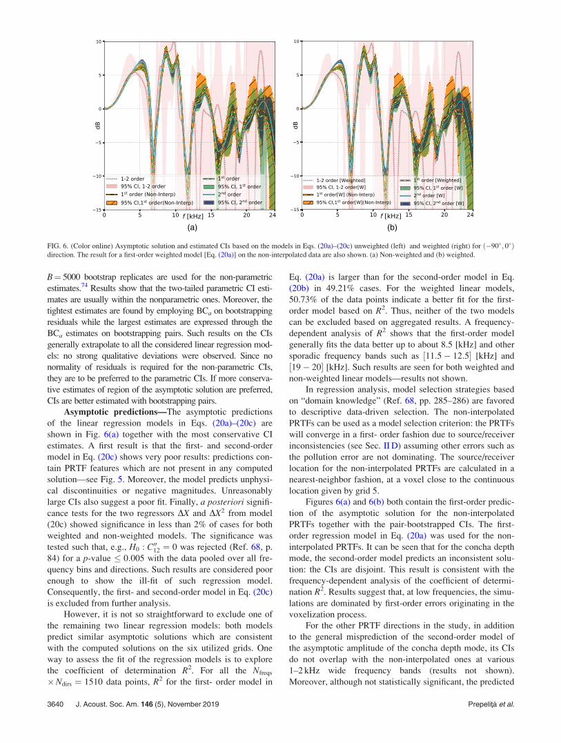
Asymptotic predictions—The asymptotic predictions

of the linear regression models in Eqs. (20a)–(20c) are

shown in Fig. 6(a) together with the most conservative CI

estimates. A first result is that the first- and second-order

model in Eq. (20c) shows very poor results: predictions con-

tain PRTF features which are not present in any computed

solution—see Fig. 5. Moreover, the model predicts unphysi-

cal discontinuities or negative magnitudes. Unreasonably

large CIs also suggest a poor fit. Finally, a posteriori signifi-

cance tests for the two regressors DX and DX2 from model

(20c) showed significance in less than 2% of cases for both

weighted and non-weighted models. The significance was

tested such that, e.g., H0 : C0012 ¼ 0 was rejected (Ref. 68, p.

84) for a p-value � 0:005 with the data pooled over all fre-

quency bins and directions. Such results are considered poor

enough to show the ill-fit of such regression model.

Consequently, the first- and second-order model in Eq. (20c)

is excluded from further analysis.

However, it is not so straightforward to exclude one of

the remaining two linear regression models: both models

predict similar asymptotic solutions which are consistent

with the computed solutions on the six utilized grids. One

way to assess the fit of the regression models is to explore

the coefficient of determination R2. For all the Nfreqs

�Ndirs ¼ 1510 data points, R2 for the first- order model in

Eq. (20a) is larger than for the second-order model in Eq.

(20b) in 49.21% cases. For the weighted linear models,

50.73% of the data points indicate a better fit for the first-

order model based on R2. Thus, neither of the two models

can be excluded based on aggregated results. A frequency-

dependent analysis of R2 shows that the first-order model

generally fits the data better up to about 8.5 [kHz] and other

sporadic frequency bands such as ½11:5� 12:5� [kHz] and

½19� 20� [kHz]. Such results are seen for both weighted and

non-weighted linear models—results not shown.

In regression analysis, model selection strategies based

on “domain knowledge” (Ref. 68, pp. 285–286) are favored

to descriptive data-driven selection. The non-interpolated

PRTFs can be used as a model selection criterion: the PRTFs

will converge in a first- order fashion due to source/receiver

inconsistencies (see Sec. II D) assuming other errors such as

the pollution error are not dominating. The source/receiver

location for the non-interpolated PRTFs are calculated in a

nearest-neighbor fashion, at a voxel close to the continuous

location given by grid 5.

Figures 6(a) and 6(b) both contain the first-order predic-

tion of the asymptotic solution for the non-interpolated

PRTFs together with the pair-bootstrapped CIs. The first-

order regression model in Eq. (20a) was used for the non-

interpolated PRTFs. It can be seen that for the concha depth

mode, the second-order model predicts an inconsistent solu-

tion: the CIs are disjoint. This result is consistent with the

frequency-dependent analysis of the coefficient of determi-

nation R2. Results suggest that, at low frequencies, the simu-

lations are dominated by first-order errors originating in the

voxelization process.

For the other PRTF directions in the study, in addition

to the general misprediction of the second-order model of

the asymptotic amplitude of the concha depth mode, its CIs

do not overlap with the non-interpolated ones at various

1–2 kHz wide frequency bands (results not shown).

Moreover, although not statistically significant, the predicted

FIG. 6. (Color online) Asymptotic solution and estimated CIs based on the models in Eqs. (20a)–(20c) unweighted (left) and weighted (right) for ð�90�; 0�Þdirection. The result for a first-order weighted model [Eq. (20a)] on the non-interpolated data are also shown. (a) Non-weighted and (b) weighted.

3640 J. Acoust. Soc. Am. 146 (5), November 2019 Prepelit�a et al.

asymptotic solution from Eq. (22) is more consistent with

the first-order model than the second-order one: one could

see small deviations in the peaks and notches of the PRTF

spectra relative to the non-interpolated PRTF.

It should be mentioned that: (i) for direction ð45�; 0�Þthe CIs overlap for the three regression models: first-order,

second-order, and non-interpolated first-order; (ii) compared

to the second-order regression model, the first-order model

fails to predict one PRTF notch for direction ð90�; 40:6�Þ:the asymptotic value of the magnitude is negative.

Figure 6(b) shows the weighted results. Results are

highly similar with the non-weighted ones in Fig. 6(a). Both

the asymptotic solutions and the CIs in the weighted case

undergo small corrections: the asymptotic solutions change

mostly less than 0.5 [dB] for the first- and second-order mod-

els while the CIs are generally smaller for the weighted mod-

els. The 0.5 [dB] value is estimated based on a histogram of

the difference for the data pooled across all frequencies and

directions—histogram not shown. All the previous results

from non-interpolated regression models are found adequate

also for the weighted regression models. Since the precision

of computed PRTFs increases with smaller voxel,18 the

weighted models are preferred over non-weighted models

and the small corrections are considered improvements in

the accuracy of predictions.

Interpolation impact—The effect of interpolation is

also seen: using interpolated PRTFs improves the precision of

the estimated asymptotic solutions. Although not shown, the

largest effect on the precision is for interpolation within the

concha volume (here, source interpolation) as compared to

interpolation in the far-field. Moreover, using the weights in

Eq. (23) appears to partly correct the prediction bias in the

asymptotic solution in Eq. (22) of the non-interpolated PRTFs

relative to the interpolated PRTFs. Consequently, since the

boundary @D gives the lowest order of convergence for the

employed discrete models, a weighted least-squares could be

used without the need to interpolate the solution if lower pre-

cision is acceptable.

Peak/Notch estimation—Of interest for the PRTF prob-

lem are the frequency locations of the peaks and notches and

their convergence. Such PRTF features were coarsely extracted

in a nearest-neighbor fashion and shown in Fig. 7 for the same

ð�90�; 0�Þ direction. Here, only the first-order model is consid-

ered. Despite the OðDf Þ error in frequency estimation, it can be

seen that such features undergo corrections of various degrees.

The amount of correction was also found to be direction-

dependent. Moreover, the individual computations could dis-

play spurious features compared to the asymptotic solution,

mostly below 20 [kHz]. Similarly, the asymptotic solution

could show extra features above 20 [kHz]—nevertheless, such

conclusion is weak since the uncertainty is high at such fre-

quencies. It is difficult to say based on the present results

whether any PRTF feature converges non-linearly in DX which

might indicate a volumetric dependence.

IV. DISCUSSION

Results in Figs. 3 and 4 show the difficulty in estimating

the computational errors in practical problems with complex

geometries: asymptotic range does not seem to be attained

even on the submillimeter grids used. Depending on fre-

quency, various sources of error and their interaction could

be responsible for such behavior—see Secs. III B 6 and II D.

Given the present models, one solution would be to increase

the computational accuracy: using double precision for

lower frequencies and smaller DX such that asymptotic range

is reached within some bandwidth. However, such solution

is presently unreachable due to restrictions in computing

memory: the simulation on grid 1 already uses more than

100� 109 voxels.

Alternatively, regression models will not only predict

the asymptotic solution, but will also reflect the quality of

such predictions: larger CIs of the asymptotic solution will

signal stronger departures from the expected asymptotic

regime—equivalently, a reliability decrease of the computed

solution. However, to avoid both prediction bias and incor-

rect CIs, the asymptotic behavior of the errors present in the

computations needs to be understood such that the correct

regression model is applied.

Since the mathematical theory predicts that the discreti-

zation error is a bias in the solution, statistical estimates for

computed solutions are sometimes discredited.23,75

Nevertheless, the discontinuity in the convergence of the

boundary @D (which may cause, e.g., jumps in the error

asymptotes47 as DX! 0) motivates the random treatment of

the convergence. Moreover, the commonly used techniques

in error estimation were shown to be difficult to apply for

the present problem and associated parameters. The esti-

mated asymptotic solutions also show that a two-grid error

estimate such as the GCI would have been unreasonably

large for the PRTF/HRTF problem. Additionally, the asymp-

totic solution was estimated based on the asymptotic behav-

ior of the discretization error of lowest order which should

persist, as DX! 0, until round-off error will cause diver-

gence from the true solution. This also motivates predictions

using least squares outside the observed grid interval: round-

off divergence would dominate the results as DX approaches

0. Finally, no noticeable divergence is qualitatively observed

at low frequencies.

Nevertheless, such regression models are not perfect.

Potential caveats in faulty model assumptions were men-

tioned in Sec. III B 4: unless the independence assumption in

the residuals is strongly violated (see, e.g., Sec. II D), the

given estimates and CIs are expected to have a reasonable

degree of reliability.

FIG. 7. (Color online) Peaks (top) and notches (bottom) on each grid in

Table III and the asymptotic solution for the first-order model in Eq. (20a).

Marker size is proportional to the log of the prominence in dB.

J. Acoust. Soc. Am. 146 (5), November 2019 Prepelit�a et al. 3641

Although the fit at higher frequencies is not much better

than a second-order model, the first-order regression model

is still considered representative for the used discrete models

since: (i) it better matches the non-interpolated predictions,

(ii) there is no previous data supporting volumetric ear

modes (most previous studies only consider distances17,76),

and (iii) it accounts for the smallest sources of error (see

Sec. II D). Besides, larger CIs could signal a poor fit.

An alternative would be to use different regression mod-

els depending on frequency but this could cause discontinu-

ous asymptotic solutions. Since pollution error could be of

concern at higher frequencies and in the spirit of more con-

servative estimates, the CIs calculated with the non-

parametric bootstrapping BCa-pairs are advised.

The present paper only deals with the quality of finite-

difference PRTF calculations and not with their validity in

predicting real-world PRTFs. Such model legitimacy needs

to be assessed in a separate validation study where FDTD

predictions along with their estimated computational errors

are compared with real-world measurements.

V. CONCLUSION

Individual computations are not necessarily a faithful

representation of wave-based formal solutions when com-

plex geometries are involved: they could embed errors which

should not be assumed negligible. The present work showed

that the current state in HRTF/PRTF simulation literature

which involve a single computation could yield erroneous

results: for each input parameter such as b, single-grid com-

puted solutions could be biased relative to the formal solu-

tion. Reliability assessment of the computational result

should always be performed.

The employed FDTD solver was verified using relevant

methods from the V&V literature—a mandatory step prior to

the investigation of the error in the simulated HRTFs/PRTFs.

The error in computed PRTFs for the ipsilateral ear was

assessed for a blocked-meatus location through a conver-

gence study on sub-millimeter grids. Since no clear asymp-

totic range was observed, the commonly employed

techniques based on Richardson extrapolation were found

inapplicable for the used grids and models. Estimates of the

asymptotic solution using weighted64 regression models fit-

ted on multiple grids were found more adequate. The method

also provides CIs for the asymptotic solutions which could

provide reliability information for any validation study. The

non-parametric bias-corrected and accelerated CI estimation

method based on bootstrapping pairs provided more conser-

vative estimates with better justified assumptions.

The estimated asymptotic solution was found less reli-

able at high frequencies and at notches in the PRTF features

even for the unprecedented grid spacing used. Moreover, the

proposed method requires a thorough understanding of the

sources of error in order to employ the correct regression

model: prediction bias is otherwise expected. In the present

case, a first-order regression model was found adequate. It

was also found that, due to the stair-stepped boundaries,

source and receiver interpolation does not appear to be

mandatory. However, interpolation improves the precision

of the estimated asymptotic solution.

Evaluation of the magnitude of the computational errors

or asymptotic estimation of the solution such as given in the

present work are a prerequisite for a correct assessment of

modeling errors and assumptions in wave-based HRTF sim-

ulations. Due to complex interactions among numerical

errors even for a simple wave model such as the SRL

scheme, using HRTF/PRTF simulations as a reliable black-

box prediction tool seems presently unfounded: no single-

grid computation is necessarily correct in the entire audible

range even when employing submillimeter voxels; error

assessment is recommended. The proposed procedure is one

such evaluation method.

ACKNOWLEDGMENTS

This research has received funding from the Academy

of Finland, Project No. 265824 and Facebook Reality Labs.

The computational resources provided by the Aalto Science-

IT project and CSC-IT Center for Science, Espoo, Finland

are also acknowledged. M.G. was supported by the

2016–2021 strategic program “Knowledge for the World” of

Aalborg University with a personal grant. S.T.P. would like

to thank all the people that shared their time and patience in

various related conversations during the long time this paper

was completed (e.g., Stefan Bilbao and Brian Hamilton from

the University of Edinburgh; Antti Hannukainen and Vesa

V€alim€aki from Aalto University). Ville Pulkki is thanked for

providing the 3D pinna mesh. Pierre Chobeau and Jonathan

Botts are thanked for commenting on very early drafts of

this manuscript. Jukka Saarelma, Terry Cho, Pablo

Hoffmann, Antti Kuusinen, and Julie Meyer are thanked for

commenting and giving useful suggestions for previous

drafts of the paper. The two anonymous reviewers are also

thanked for their useful comments and corrections.

APPENDIX A: MATHEMATICAL SYMBOLS ANDCONVENTIONS

In the present text, the lattice that the FDTD update

operates upon and tessellates the space-time will be referred

to as grid while the term mesh will denote any triangulated

representation of a continuous surface. A uniform and struc-

tured 3D Cartesian grid is used, formed by cubic control vol-

umes which are named voxels in the present work. The grid

spacing will be denoted by DX, the time step by DT, and the

“sampling” frequency as fs ¼ 1=DT.

The term model is used throughout the work in a broad

sense as a representation of some system/process or even

another model without circular “referencing”—see also the

AIAA definition (Ref. 20, p. 92).

Signals in the frequency domain are denoted by upper-

case letters while lowercase letters are used for their time-

domain representation. The FDTD and semi-discrete [e.g.,

PjðtÞ in Eq. (5)] dependent variables are written in uppercase

and the superscript indexes time while the subscript indexes

integer 3D lattice coordinates.

3642 J. Acoust. Soc. Am. 146 (5), November 2019 Prepelit�a et al.

Parentheses are used for arguments in the case of contin-

uous signals, while square brackets are used for discrete sig-

nals. X is used for the angular frequency [rad/s] for

continuous temporal signals, while x is for the angular fre-

quency of discrete-time signals. The set of natural numbers

is denoted by N (with N :¼N� f0g), integer numbers by

Z and R denotes the set of real numbers.

Contrary to the notation in the PDE literature, indepen-

dent variables as subscripts to dependent variables are used

as naming conventions: pt 6¼ @p=@t while @tp ¼ @p=@t.

APPENDIX B: SOFTWARE AND HARDWARE DETAILS

The FDTD implementation was developed on the GPU

using CUDA kernels77 and parallelized further using the

MPI using a CUDA-aware MPI library.78

For the voxelization process, all triangle-voxel intersec-

tions are done in double precision. All FDTD simulations

are done in single precision while the post-processing (such

as the SciPy79 v1.1.0 FFT algorithms) is implemented in

Python 2.7.13 [Enthought Canopy (Version 2.1.9) Software,

http://www.enthought.com] by using double precision

NumPy80 v1.15.4 arrays. For code verification, the analytical

terms (i.e., initial conditions and forcing terms) are initially

calculated in double precision.

For solution verification, the single term expansion with

unknown qobs from Eca and Hoekstra64 is calculated naively

by sweeping qobs in Dqobs ¼ 0:005 steps and finding zero-

crossing (including zeros) for the last non-linear equation in

Appendix B.2 from the same work. The Box-Tidwell proce-

dure is based on Fox’s (Ref. 81, p. 312) R version (using a

tolerance of 10�3 and a maximum of 1000 steps). For the

weighted Box-Tidwell calculation, the ordinary least squares

calls from the two fits used by the procedure are replaced

by weighted least squares fits on the same data with the

weights from Eq. (23). The linear regression prediction is

based on the results from statsmodel82 (Version 0.8.0)

while the non-linear regression trials were done using the

scipy.optimize package (using the Levenberg-Marquardt

algorithm and explicitly defining the Jacobian). The

scipy.signal.find_peaks() function is used to extract the fea-

tures in Fig. 7 (feature height of 30 dB and width of Df ).

The BCa bootstrapped CIs are computed by employing

scikits.bootstrap (Version 1.0.0) python package (http://

github.org/cgevans/scikits-bootstrap) which is based on the

description given in Chap. 14 by Efron and Tibshirani.70

The final simulations were run on Amazon EC2 on

p2.16xlarge instances running CentOS 7.3 in the same place-

ment group. Each instance contained 16 NVIDIA K80

GPUs, totaling 16� 12¼ 192 GB GPU memory per node.

The relevant software stack on the cluster consisted of gcc4.8.5, CUDA toolkit 8.0, and OpenMPI 2.0.2. Synchronous

MPI communication was used to avoid non-determinism

concerns.83

1P. M. Hofman, J. G. A. Van Riswick, and A. J. Van Opstal, “Relearning

sound localization with new ears,” Nat. Neurosci. 1(5), 417–421 (1998).2E. M. Wenzel, M. Arruda, D. J. Kistler, and F. L. Wightman,

“Localization using nonindividualized head-related transfer functions,”

J. Acoust. Soc. Am. 94(1), 111–123 (1993).

3A. J. Hoogstrate, H. Van Den Heuvel, and E. Huyben, “Ear identification

based on surveillance camera images,” Sci. Justice 41(3), 167–172 (2001).4M. Morimoto and Y. Ando, “On the simulation of sound localization,”

J. Acoust. Soc. Jpn. (e) 1(3), 167–174 (1980).5F. L. Wightman and D. J. Kistler, “Headphone simulation of free-field lis-

tening. II: Psychophysical validation,” J. Acoust. Soc. Am. 85(2),

868–878 (1989).6E. H. A. Langendijk and A. W. Bronkhorst, “Fidelity of three-dimen-

sional-sound reproduction using a virtual auditory display,” J. Acoust.

Soc. Am. 107(1), 528–537 (2000).7R. L. Martin, K. I. McAnally, and M. A. Senova, “Free-field equivalent

localization of virtual audio,” J. Audio Eng. Soc. 49(1/2), 14–22 (2001).8P. Majdak, P. Balazs, and B. Laback, “Multiple exponential sweep method

for fast measurement of head-related transfer functions,” J. Audio Eng.

Soc. 55(7/8), 623–637 (2007).9P. Dietrich, B. Masiero, and M. Vorl€ander, “On the optimization of the

multiple exponential sweep method,” J. Audio Eng. Soc. 61(3), 113–124

(2013).10G. Enzner, “3d-continuous-azimuth acquisition of head-related impulse

responses using multi-channel adaptive filtering,” in 2009 IEEE Workshopon Applications of Signal Processing to Audio and Acoustics, New Paltz,

NY (2009), pp. 325–328.11B. F. G. Katz, “Boundary element method calculation of individual head-

related transfer function. I. Rigid model calculation,” J. Acoust. Soc. Am.

110(5), 2440–2448 (2001).12Y. Kahana and P. A. Nelson, “Numerical modelling of the spatial acoustic

response of the human pinna,” J. Sound Vib. 292(1–2), 148–178 (2006).13W. Kreuzer, P. Majdak, and Z. Chen, “Fast multipole boundary element

method to calculate head-related transfer functions for a wide frequency

range,” J. Acoust. Soc. Am. 126(3), 1280–1290 (2009).14C. Jin, P. Guillon, N. Epain, R. Zolfaghari, A. van Schaik, A. Tew, C.

Hetherington, and J. Thorpe, “Creating the Sydney York morphological

and acoustic recordings of ears database,” IEEE Trans. Multimed. 16(1),

37–46 (2014).15H. Ziegelwanger, P. Majdak, and W. Kreuzer, “Numerical calculation of

listener-specific head-related transfer functions and sound localization:

Microphone model and mesh discretization,” J. Acoust. Soc. Am. 138(1),

208–222 (2015).16T. Xiao and Q. H. Liu, “Finite difference computation of head-related

transfer function for human hearing,” J. Acoust. Soc. Am. 113(5),

2434–2441 (2003).17P. Mokhtari, H. Takemoto, R. Nishimura, and H. Kato, “Frequency and

amplitude estimation of the first peak of head-related transfer functions

from individual pinna anthropometry,” J. Acoust. Soc. Am. 137(2),

690–701 (2015).18S. Prepelit�a, M. Geronazzo, F. Avanzini, and L. Savioja, “Influence of

voxelization on finite difference time domain simulations of head-related

transfer functions,” J. Acoust. Soc. Am. 139(5), 2489–2504 (2016).19P. J. Roache, Verification and Validation in Computational Science and

Engineering (Hermosa Publishers, Albuquerque, NM, 1998).20W. L. Oberkampf and C. J. Roy, Verification and Validation in Scientific

Computing, 1st ed. (Cambridge University Press, New York, 2010).21D. Lee and T.-S. Ahn, “A boundary element model for acoustic responses

in the ear canal and its statistical validation and updating,” J. Mech. Sci.

Technol. 28(4), 1203–1217 (2014).22V. R. Algazi, C. Avendano, and R. O. Duda, “Elevation localization and

head-related transfer function analysis at low frequencies,” J. Acoust. Soc.

Am. 109(3), 1110–1122 (2001).23W. L. Oberkampf, T. G. Trucano, and C. Hirsch, “Verification, validation,

and predictive capability in computational engineering and physics,”

Appl. Mech. Rev. 57(5), 345–384 (2004).24S. Bilbao, “Modeling of complex geometries and boundary conditions in

finite difference/finite volume time domain room acoustics simulation,”

IEEE Trans. Audio, Speech, Lang. Process. 21(7), 1524–1533 (2013).25A. D. Pierce, Acoustics: An Introduction to Its Physical Principles and

Applications (Acoustical Society of America, Woodbury, New York,

1989).26P. M. Morse and K. U. Ingard, Theoretical Acoustics (Princeton

University Press, Princeton, NJ, 1986).27K. Kowalczyk and M. van Walstijn, “Formulation of a locally reacting

wall in finite difference modelling of acoustic spaces,” in Proceedings ofthe International Symposium on Room Acoustics (ISRA), Seville, Spain

(2007), pp. 1–6.

J. Acoust. Soc. Am. 146 (5), November 2019 Prepelit�a et al. 3643

28C. Webb and S. Bilbao, “Computing room acoustics with CUDA—3d

FDTD schemes with boundary losses and viscosity,” in 2011 Proceedingsof the IEEE International Conference on Acoustics, Speech, and SignalProcessing (ICASSP), Prague, Czech Republic (2011), pp. 317–320.

29J. Sheaffer, M. V. Walstijn, and B. Fazenda, “Physical and numerical con-

straints in source modeling for finite difference simulation of room

acousticsa),” J. Acoust. Soc. Am. 135(1), 251–261 (2014).30D. Cohen-Or and A. Kaufman, “Fundamentals of surface voxelization,”

Graph. Models Image Process. 57(6), 453–461 (1995).31In the present work, the commonly-used term error is chosen in favor of

uncertainty despite some inherent practical drawbacks. A further discus-

sion is out of scope—see, e.g., Sec. 2.4 from the text by Oberkampf and

Roy (Ref. 20).32R. Holland, “Pitfalls of staircase meshing,” IEEE Trans. Electromagn.

Compat. 35(4), 434–439 (1993).33E. Hairer, S. P. Nørsett, and G. Wanner, Solving Ordinary Differential

Equations I: Nonstiff Problems, 2nd ed. (1993), corr. 3rd ed. (Springer,

Heidelberg, London, 2009).34To explore the spatio-temporal dependence of both principal error terms, one

can invoke the (multiplicative) separation of variables in Cartesian coordi-

nates and apply the asymptotic expansion of the error independently. For

instance, for the 3D wave equation on a Cartesian grid of uniform spacing

DX, a “separated” solution is of the form pðr; tÞ ¼ ptðtÞpxðxÞpyðyÞpzðzÞyielding a second-order simulated solution epðr; t;DT;DXÞ ¼ eptðt;DTÞepxðx;DXÞepyðy;DXÞ epzðz;DXÞ ¼ pðr; tÞ þ �pðtÞpxðxÞpyðyÞpzðzÞDT2 þ �rðrÞptðtÞDX2 þ HOT where �rðrÞ ¼ pxðxÞpzðzÞ�yðyÞ þ pxðxÞpyðyÞ�zðzÞ þ pyðyÞpzðzÞ�xðxÞ.

35C. J. Roy, “Review of code and solution verification procedures for com-

putational simulation,” J. Comput. Phys. 205(1), 131–156 (2005).36R. May and J. Noye, “The numerical solution of ordinary differential

equations: Initial value problems,” North-Holland Math. Stud. 83, 1–94

(1984).37J. Botts and L. Savioja, “Spectral and pseudospectral properties of finite

difference models used in audio and room acoustics,” IEEE/ACM Trans.

Audio, Speech, Lang. Process. 22(9), 1403–1412 (2014).38J. C. Strikwerda, Finite Difference Schemes and Partial Differential

Equations, 2nd ed. (SIAM, Philadelphia, PA, 2004).39See equivalent spatial/volumetric arguments in the work by Botts and

Savioja (Ref. 57).40J. T. Oden, S. Prudhomme, and L. Demkowicz, “A posteriori error estima-

tion for acoustic wave propagation problems,” Arch. Comput. Methods

Eng. 12(4), 343–389 (2005).41J. Botts, A. Bockman, and N. Xiang, “On the selection and implementa-

tion of sources for finite-difference methods,” in Proceedings of the 20thInternational Congress on Acoustics, Sydney, Australia (2010), pp.

593:1–593:5.42J. H€aggblad and O. Runborg, “Accuracy of staircase approximations in

finite-difference methods for wave propagation,” Numer. Math. 128(4),

741–771 (2014).43A. C. Cangellaris and D. B. Wright, “Analysis of the numerical error

caused by the stair-stepped approximation of a conducting boundary in

FDTD simulations of electromagnetic phenomena,” IEEE Trans.

Antennas Prop. 39(10), 1518–1525 (1991).44The dependence on frequency stems from, e.g., phase/group delay consid-

erations. For a given angular frequency x, a phase error will translate in

the complex frequency plane as an arc-error of length �ph ¼ xsg (mod 2p)

where sg is (for the PRTF solution) the temporal delay error that will

behave as OðDXÞ=c. Thus, �ph ¼ xOðDXÞ=c. Note that, besides the rela-

tive orientation of the boundary surface to the grid, the principal error con-

stants for the first-order phase errors also depend on, e.g., the angle of

incidence of the incoming (assumed-plane) wave to the (continuous)

boundary (Ref. 43).45P. Luizard, M. Otani, J. Botts, L. Savioja, and B. F. Katz, “Comparison of

sound field measurements and predictions in coupled volumes between

numerical methods and scale model measurements,” Proc. Mtgs. Acoust.

19, 015114 (2013).46S. Bilbao, B. Hamilton, J. Botts, and L. Savioja, “Finite volume time

domain room acoustics simulation under general impedance boundary

conditions,” IEEE/ACM Trans. Audio, Speech, Lang. Process. 24(1),

161–173 (2016).47The argument can be (roughly) sketched by fixing the boundary geometry

@ eDðDXÞ ¼ @ eDðDXiÞ :¼ eD i, with DXi > 0 and eD i 6¼ @D, i.e., there are

geometrical errors in the discrete boundary eD i. Ignoring all other sources

of error, for each fixed eD i and angular frequency x, we can perform an

asymptotic expansion of the computed solution: ePr½x� ¼ Pr;i½x�þ �r;i½x�DX

minðg;qÞi þ HOT. Wave phenomena dictate that Pr;i is the true/

sought continuous solution Pr as x=c! 0, e.g., we can write an asymp-

totic expansion in x for the boundary-induced error ei½x� ¼ Pr;i½x��Pr½x�. ei½x� might also propagate in the discretization error terms (e.g.,

�r;i½x�), depending on x, the topology of the continuous boundary @D and

the update scheme. Here, non-physical solutions such as DC are ignored.

In practical simulations, due to the (re-)voxelization process, as the grid is

refined (i.e., DX ! 0), Pr;i½x� is expected to change with DX by lowering

ei½x� which in turn will lower the corresponding propagated part in �r;i (for

fixed x). Moreover, most of such frequencies will not propagate in the

update due to the Nyquist-Shannon sampling criterion.48J. H€aggblad and B. Engquist, “Consistent modeling of boundaries in

acoustic finite-difference time-domain simulations,” J. Acoust. Soc. Am.

132(3), 1303–1310 (2012).49A.-K. Tornberg and B. Engquist, “Consistent boundary conditions for the

Yee scheme,” J. Comput. Phys. 227(14), 6922–6943 (2008).50B. Hamilton, “Finite volume perspectives on finite difference schemes and

boundary formulations for wave simulation,” in Proceedings of the 17thInternational Conference on Digital Audio Effects (DAFx-14), Erlangen,

Germany (2014), pp. 295–302.51K. Salari and P. Knupp, “Code verification by the method of manufactured

solutions,” SAND2000-1444, Sandia National Labs., Albuquerque, NM;

Sandia National Labs., Livermore, CA (2000).52P. M. Morse, “Some aspects of the theory of room acoustics,” J. Acoust.

Soc. Am. 11(1), 56–66 (1939).53F. V. Hunt, L. L. Beranek, and D. Y. Maa, “Analysis of sound decay in

rectangular rooms,” J. Acoust. Soc. Am. 11(1), 80–94 (1939).54E. W. Cheney and W. A. Light, “Tensor product interpolation,” in A

Course in Approximation Theory (American Mathematical Society,

Pacific Grove, CA, 2009), pp. 46–50.55T. I. Laakso, V. Valimaki, M. Karjalainen, and U. K. Laine, “Splitting the

unit delay [FIR/all pass filters design],” IEEE Signal Process. Mag. 13(1),

30–60 (1996).56M. Rosenfeld, “Grid refinement test of time-periodic flows over bluff bod-

ies,” Comput. Fluids 23(5), 693–709 (1994).57J. Botts and L. Savioja, “Effects of sources on time-domain finite differ-

ence models,” J. Acoust. Soc. Am. 136(1), 242–247 (2014).58The convergence of such geometric series is satisfied when

DX2jEX;ref ½r1;x� þ ET;ref ½r1;x�k2C=c2j < jPref ½r1;x�j, where DX; kC , and c

are all from the free-field simulation. Thus, the series is convergent for a

sub-unitary relative (mainly spatial) discretization error of the free-field

simulation; alternatively, for DX sufficiently small (i.e., solution is within

the asymptotic range). A small discretization error is obtained for diagonal

directions or for lower frequencies f � fs [see the dispersion error analysis

for the used (interior) update (Ref. 85) and/or truncation error analysis for

the used difference operators]. Thus, if DX is not small enough, Eq. (13)

could be inaccurate for directions closer to axial directions of the grid, for

higher frequencies x and for far-field (i.e., large jr1j).59T. Xing and F. Stern, “Factors of safety for Richardson extrapolation,”

J. Fluids Eng. 132(6), 061403:1 (2010).60A. V. Oppenheim and C. J. Weinstein, “Effects of finite register length in

digital filtering and the fast Fourier transform,” Proc. IEEE 60(8),

957–976 (1972).61L. Trefethen and J. Weideman, “The exponentially convergent trapezoidal

rule,” SIAM Rev. 56(3), 385–458 (2014).62F. Stern, R. Wilson, and J. Shao, “Quantitative V&V of CFD simulations

and certification of CFD codes,” Int. J. Numer. Meth. Fluids 50(11),

1335–1355 (2006).63D. C. Baird, Experimentation: An Introduction to Measurement Theory

and Experiment Design, 3rd ed. (Addison-Wesley, Englewood Cliffs, NJ,

1994).64L. Eca and M. Hoekstra, “A procedure for the estimation of the numerical

uncertainty of CFD calculations based on grid refinement studies,”

J. Comput. Phys. 262, 104–130 (2014).65F. G. Blottner, “Influence of boundary approximations and conditions on

finite-difference solutions,” J. Comput. Phys. 48(2), 246–269 (1982).66D. L. Potter, F. G. Blottner, A. R. Black, C. J. Roy, and B. L.

Bainbridge, “Visualization of Instrumental Verification Information

Details (VIVID): Code development, description, and usage,” SAND

2005-1485, Sandia National Laboratories, Albuquerque, New Mexico

(2005).

3644 J. Acoust. Soc. Am. 146 (5), November 2019 Prepelit�a et al.

67G. E. P. Box and P. W. Tidwell, “Transformation of the independent varia-

bles,” Technometrics 4(4), 531–550 (1962).68D. C. Montgomery, E. A. Peck, and G. G. Vining, Introduction to

Linear Regression Analysis, 4th ed. (Wiley-Interscience, Hoboken, NJ,

2006).69J. O. Rawlings, S. G. Pantula, and D. A. Dickey, Applied Regression

Analysis: A Research Tool, Springer Texts in Statistics, 2nd ed. (Springer-

Verlag, New York, 1998).70B. Efron and R. J. Tibshirani, An Introduction to the Bootstrap (Chapman

and Hall/CRC, New York, NY, 1994).71L. E. Kinsler, F. R. Austin, C. B. Alan, and S. V. James, Fundamentals of

Acoustics, 4th ed. (Wiley, New York, 2000).72J. O. Smith, Mathematics of the Discrete Fourier Transform (DFT): With

Audio Applications, 2nd ed. (W3K Publishing, 2007).73E. A. G. Shaw and R. Teranishi, “Sound pressure generated in an external-

ear replica and real human ears by a nearby point source,” J. Acoust. Soc.

Am. 44(1), 240–249 (1968).74D. W. K. Andrews and M. Buchinsky, “On the number of bootstrap repeti-

tions for BCA confidence intervals,” Econom. Theory 18(4), 962–984

(2002).75W. L. Oberkampf and T. G. Trucano, “Verification and validation in com-

putational fluid dynamics,” Prog. Aerosp. Sci. 38(3), 209–272 (2002).76P. Mokhtari, H. Takemoto, R. Nishimura, and H. Kato, “Vertical normal

modes of human ears: Individual variation and frequency estimation from

pinna anthropometry,” J. Acoust. Soc. Am. 140(2), 814–831 (2016).

77J. Saarelma and L. Savioja, “An open source finite difference time-domain

solver for room acoustics using Graphics Processing Units,” in

Proceedings of the Forum Acusticum, European Acoustics Association,

Krakow, Poland (2014), pp. 1–6.78“CUDA-Aware OpenMPI distribution” (2018), https://www.open-mpi.

org/faq/?category=runcuda (Last viewed March 10, 2018).79E. Jones, T. Oliphant, and P. Peterson, “${$scipy$}$: Open source scien-

tific tools for ${$python$}$” (2014), url: http://www.scipy.org/ (Last

accessed February 1, 2019).80S. V. d. Walt, S. C. Colbert, and G. Varoquaux, “The NumPy array: A

structure for efficient numerical computation,” Comput. Sci. Eng. 13(2),

22–30 (2011).81J. Fox and S. Weisberg, An R Companion to Applied Regression, 2nd ed.

(SAGE Publications, Inc., Thousand Oaks, CA, 2010).82S. Seabold and J. Perktold, “Statsmodels: Econometric and statistical

modeling with python,” in Proceedings of the 9th Python in Science

Conference, SciPy Society, Austin, TX (2010), pp. 57–61.83G. Gopalakrishnan, R. M. Kirby, S. Siegel, R. Thakur, W. Gropp, E. Lusk,

B. R. De Supinski, M. Schulz, and G. Bronevetsky, “Formal analysis of

MPI-based parallel programs,” Commun. ACM 54(12), 82–91 (2011).84B. Gustafsson, H.-O. Kreiss, and J. Oliger, Time-Dependent Problems and

Difference Methods, 2nd ed. (Wiley, Hoboken, NJ, 2013).85K. Kowalczyk and M. van Walstijn, “Room acoustics simulation using 3-

D compact explicit FDTD schemes,” IEEE Trans. Audio, Speech, Lang.

Process. 19(1), 34–46 (2011).

J. Acoust. Soc. Am. 146 (5), November 2019 Prepelit�a et al. 3645