physics of the upper polar atmosphere - readingsample
TRANSCRIPT

Springer Atmospheric Sciences
Physics of the Upper Polar Atmosphere
Bearbeitet vonAsgeir Brekke
1. Auflage 2012. Buch. xxvi, 386 S. HardcoverISBN 978 3 642 27400 8
Format (B x L): 16,8 x 24 cmGewicht: 931 g
Weitere Fachgebiete > Geologie, Geographie, Klima, Umwelt > Geologie undNachbarwissenschaften > Geophysik
Zu Inhaltsverzeichnis
schnell und portofrei erhältlich bei
Die Online-Fachbuchhandlung beck-shop.de ist spezialisiert auf Fachbücher, insbesondere Recht, Steuern und Wirtschaft.Im Sortiment finden Sie alle Medien (Bücher, Zeitschriften, CDs, eBooks, etc.) aller Verlage. Ergänzt wird das Programmdurch Services wie Neuerscheinungsdienst oder Zusammenstellungen von Büchern zu Sonderpreisen. Der Shop führt mehr
als 8 Millionen Produkte.

2
The atmosphere of the Earth
2.1 NOMENCLATURE
The atmosphere of the Earth is an ocean of gas encircling the globe. It stretchesout far from the surface; how far out is a question of definition.
In Figure 2.1 we have illustrated schematically the variation of some charac-teristic parameters up to an altitude of 450 km. There are rather strong variationsin the upper atmosphere above 100 km during a solar cycle, and this is illustratedin the figure by curves representing average solar maximum and minimum con-ditions. The cross-hatched areas between these curves illustrate the variability ofthe parameters. The number density (n) of the atmosphere decreases monotonic-ally with height from 1025 m�3 at ground level to 1014 m�3 at 400 km. The atomicmass number is constant and close to 30 at the ground and up to about 100 km;above that region it decreases gradually toward 15 at 400 km. This corresponds toan air density of 1.2 kg/m3 at ground level decreasing to about 3.4� 10�6 kg/m3 at90 km, 2.4� 10�8 kg/m3 at 120 km, and 2.8� 10�10 kg/m3 at 200 km, respectively.According to variations in its composition the atmosphere is divided into twomain regions, the homosphere and the heterosphere, indicating that below 100 kmthe gas constituents are fully mixed into a homogeneous gas. Above this height,however, the different constituents behave independently, and the atmosphere isheterogeneous.
The temperature (T) of the atmosphere has a more complicated behavior withheight. It starts out by decreasing in the troposphere from about 290K at theground and reaching a minimum close at 215K at 1,520 km, called the tropopause.
Above the tropopause is the stratosphere, and here the temperature increasesup to a maximum of close to 280K, called the stratopause, usually situated closeto 50 km. Above the stratopause the temperature decreases again in the meso-sphere and reaches the lowest temperature in the atmosphere in the mesopause,usually situated at about 70–90 km. The temperature in the mesopause may be as
A. Brekke, Physics of the Upper Polar Atmosphere, Springer Praxis Books, 51DOI 10.1007/978-3-642-27401-5_2, © pringer-Verlag erlin Heidelberg 2013 GmbH B S

low as 160K or even lower at occasions. As a curiosity, however, the mesopausetemperature in polar regions is higher in winter than in summer.
Above the mesopause the temperature increases dramatically in thethermosphere where temperatures of more than 1,000K can be found above theexobase indicated in Figure 2.1 at 400 km. Above this region the temperature isfairly constant by height, but may vary considerably by time.
The nomenclature used for characterizing different areas in the atmosphererefers to either temperature, composition, or dynamics. At the ground we findthat the atmosphere is composed of close to 80% N2 and 20% O2, while thecontribution from other gases is less than 1%. This mixture holds all the way upto about 100 km. The region below 100 km is therefore called the homosphere orthe turbosphere. The latter reflects the fact that turbulence causes the mixture.Above 100 km, molecules start to dissociate and become more independent ofeach other; they are more heterogeneous. This region is therefore called the hetero-sphere or the barosphere; the latter reflecting the fact that the different species havedifferent scale heights or barometric heights.
52 The atmosphere of the Earth [Ch. 2
Figure 2.1. Model height profiles of the temperature T , density n, molecular massM, and scale
height H distributions in the Earth’s atmosphere below 450 km. The different regions are also
indicated by their characteristic names according to temperature or composition. Variability in
the different parameters with respect to solar activity is indicated by the hatched areas.

In Figure 2.2 we show a more detailed presentation of the altitude profiles ofdifferent atmospheric species between 1,000 km and the ground under solarminimum and maximum conditions. While atomic oxygen dominates the upperatmosphere above 250 km under solar maximum conditions, hydrogen is moredominant above 400 km under solar minimum conditions. Below 200 km,however, molecular oxygen and nitrogen together with argon are the dominantspecies independent of solar activity.
Due to the composition at ground level (80% N2 and 20% O2) the averagemolecular mass will be 28.8 a.m.u. Since molecules start to dissociate above about100 km and nitrogen molecules dissociate faster than oxygen molecules, the molec-ular weight will decrease and oxygen atoms will be the dominant species from400 km to above 1,000 km, at least during solar cycle maximum (see Figure 2.2 forreferences).
At 600 km where we might have 84% O and 16% He, the molecular mass is14 a.m.u. While the number density at the ground is about 2.5� 1025 m�3, it isabout 1019 m�3 at 100 km, and at 200 km it has been reduced to about 1016 m�3.The density therefore has decreased by more than 109 from the ground up totypical rocket trajectories.
2.2 TEMPERATURE STRUCTURE OF THE ATMOSPHERE
The temperature in the atmosphere decreases quite monotonically up to thetropopause. This is due to the fact that infrared radiation from the ground, which
2.2 Temperature structure of the atmosphere 53]Sec. 2.2
Figure 2.2. Composition changes in the atmosphere with respect to (a) solar minimum and
(b) solar maximum conditions showing the dominance of heavier constituents at larger altitudes
during solar maximum. (From U.S. Standard Atmosphere, 1976.)

is absorbed in the atmosphere, is rather constant because the surface temperatureof the globe is constant, and therefore the heat expands out in the atmosphere inradial directions. The heat will then be distributed into larger and larger volumesand therefore the temperature must decrease.
Due to the ozone layer situated between 5 and 40 km above the grounddepending on latitude (Figure 2.3) which absorbs a large portion of the solar radi-ation between 200 and 300 nm, the atmosphere becomes heated in the stratosphereand the temperature increases. Above the stratopause, however, the heat balanceresults in excess outward radiation again, and the temperature decreases rapidly inthe mesosphere until the sharp minimum occurs at the mesopause.
By observing the ozone density profile at different latitudes, however, the peakaltitude is found to decrease and the peak magnitude to increase with increasinglatitude. More ozone is therefore present at lower altitudes (<25 km) in the polarregion (Figure 2.3).
This is even more clearly brought out in Figure 2.4 where the latitudinalaverage of the ozone content at different altitudes below 50 km is presented versusthe latitude for the average February month. The winter pole has rather highozone content at low altitudes (<20 km) while the ozone density above theequator is much smaller and maximizes above 20 km. This latter effect cannot beexplained by the simple photochemical equilibrium models of the atmosphere sincefrom these we would expect the ozone content to be high at lower heights in theequatorial region where the solar radiation and the radiative dissociation of O2 ishighest. Transport processes must therefore be of fundamental importance forglobal ozone distribution.
In Figure 2.5 the latitudinal distribution of total ozone content for differentseasons of the year is presented. Again there are clear maxima above the polarregions, but it is seen that these maxima occur in spring. The maximum in the
54 The atmosphere of the Earth [Ch. 2
Figure 2.3. Ozone density profiles in the atmosphere at different latitudes in the northern
hemisphere. The concentration is given in molecules per cm3. (After Shimazaki, 1987.)

2.2 Temperature structure of the atmosphere 55]Sec. 2.2
Figure 2.4. Latitudinally averaged ozone distribution for February shown as a function of
height and latitude. A strong maximum is observed below 20 km in the Arctic region. (From
Dutsch, 1978.)
Figure 2.5. Latitudinal and seasonal variation of the total ozone content. The labels added to
the isolines are given in Dobson units. (From London, 1985.)
northern hemisphere in March is about 15% higher than the correspondingmaximum in the southern hemisphere in October.
In the northern hemisphere the amplitudes of seasonal variation are alsolarger, varying from a maximum of close to 460 Dobson units in April at times toabout 280 Dobson units in November. That is a variation of more than 20%around the mean value.
The total ozone content in a vertical column above a ground-based observerhas been measured for more than 50 years at different places on Earth.
The term ‘‘total ozone’’, sometimes referred to as total layer thickness, thusrepresents the height integral of the column density and is often abbreviated asatm-cm or cm (STP). This corresponds to the thickness of the layer if the pressureand density were reduced to standard atmospheric values throughout the layer.The Dobson unit is derived in a similar manner and abbreviated as m-atm-cmwhich equals 10�3 atm-cm. Therefore, 300 Dobson units represent an ozonecontent which, when reduced to standard temperature and pressure throughoutthe layer, would correspond to a column of 3mm.
One of the early findings in the research of ozone was the smaller amount ofozone in the Antarctic spring than in the Arctic spring. Another early result ofsuch measurements was the occasional decrease observed in total ozone during theearly springtime.
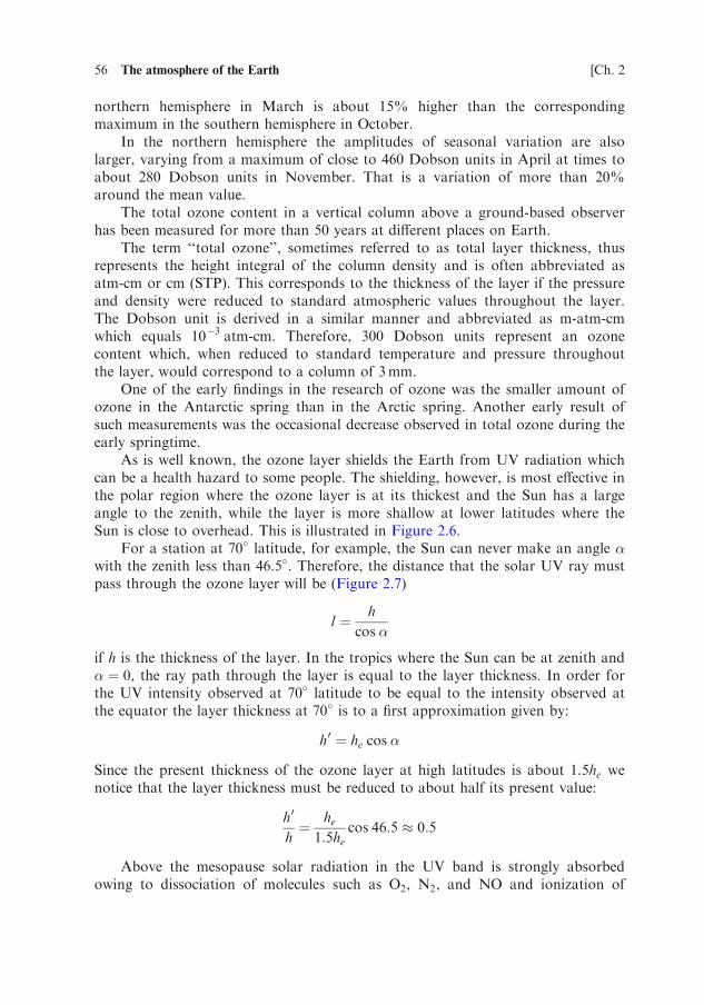
As is well known, the ozone layer shields the Earth from UV radiation whichcan be a health hazard to some people. The shielding, however, is most effective inthe polar region where the ozone layer is at its thickest and the Sun has a largeangle to the zenith, while the layer is more shallow at lower latitudes where theSun is close to overhead. This is illustrated in Figure 2.6.
For a station at 70� latitude, for example, the Sun can never make an angle �with the zenith less than 46.5�. Therefore, the distance that the solar UV ray mustpass through the ozone layer will be (Figure 2.7)
l ¼ h
cos �
if h is the thickness of the layer. In the tropics where the Sun can be at zenith and� ¼ 0, the ray path through the layer is equal to the layer thickness. In order forthe UV intensity observed at 70� latitude to be equal to the intensity observed atthe equator the layer thickness at 70� is to a first approximation given by:
h 0 ¼ he cos �
Since the present thickness of the ozone layer at high latitudes is about 1.5he wenotice that the layer thickness must be reduced to about half its present value:
h 0
h¼ he
1:5hecos 46:5 � 0:5
Above the mesopause solar radiation in the UV band is strongly absorbedowing to dissociation of molecules such as O2, N2, and NO and ionization of
56 The atmosphere of the Earth [Ch. 2

2.2 Temperature structure of the atmosphere 57]Sec. 2.2
Figure 2.6. A schematic illustration of the global ozone distribution showing a thinning of the
layer at lower latitudes where also solar irradiation can have a vertical impact on the atmo-
sphere. The height of the maximum in the layer, however, is larger at equatorial regions than at
the poles.
Figure 2.7. Illustration of variation in the length of the ray path through the ozone layer with a
varying solar zenith angle.

atomic oxygen and other molecules and atoms. This leads to a new temperatureincrease which is particularly strong up to about 400 km.
The very strong absorption of UV radiation in the thermosphere, however, isaccompanied by strong variability in the temperature of this region as illustratedin Figure 2.1. This is because solar UV radiation itself is so variable. As the tem-perature above 400–600 km appears fairly constant with height as a function ofaltitude, it is often referred to as the exospheric temperature (T1). Figure 2.8,which is an alternative presentation of Figure 2.1 above 100 km, shows the rangeof variability in thermospheric temperature at different altitudes in the course of asolar cycle due to variations in the exospheric temperature. The intensity index ofsolar radio emission at F10:7 is used as a reference parameter to the solar cycle.The value 50 represents solar minimum conditions while the value 200 representssolar maximum conditions.
The exospheric temperature can change by 600K or more during a solar cycleaccording to similar model calculations (as presented in Figure 2.8).
The thermospheric temperature, however, is not constant all over the globeand exhibits a seasonal variation. The thermospheric temperature at 300 km as afunction of latitude for solstice and equinox conditions is presented in Figure 2.9.Also shown in Figure 2.9 is the mean molecular mass (a.m.u.) for the correspond-ing conditions. At solstice especially, latitudinal variations are as large as thetemperature changes from close to 1,400K at the summer pole to slightly above900K at the winter pole, and the molecular mass changes from 21 a.m.u. to17 a.m.u. in the same region.
58 The atmosphere of the Earth [Ch. 2
Figure 2.8. Variability in the thermospheric temperature for different values of the solar radio
flux index (F10:7) in units of 10�22 Wm�2 Hz�1 reduced to 1AU. Under average solar minimum
and maximum conditions the F10:7 index is 50 and 200, respectively. (From Roble, 1987.)

The consequence of this is that heavier molecules are brought up to higheraltitudes from below in the summer hemisphere and downward in the winter hemi-sphere (Figure 2.10). The summer thermosphere at 300 km and above is thereforedominated by N2 molecules, while the winter thermosphere in the same heightregion has a large contribution of helium atoms.
The thermospheric temperature also responds to solar variations on a shortertime scale than solar cycles or seasonal periods. Figure 2.11 presents a comparisonof variations in exospheric temperature T1, atmospheric mass density �, solarradio emission flux S (¼ F10:7), and a geomagnetic index Ap. The latter representsvariations in the Earth’s magnetic field. presumably due to ionospheric currents.
The 27-day period in solar radio emission, S (F10:7), is clearly reflected in T1as well as �, as if the atmosphere is expanding and contracting as the solar fluxincreases and decreases.
2.3 ATMOSPHERIC DRAG ON SATELLITES
Figure 2.12 gives a schematic presentation of the variability of atmospheric densitybetween 100 and 1,000 km under solar maximum and minimum conditions as wellas under extreme solar maximum daytime conditions. Density variations of twoorders of magnitude can in fact take place during a solar cycle above 400 kmaltitude.
2.3 Atmospheric drag on satellites 59]Sec. 2.3
Figure 2.9. Latitudinal distribution of the neutral temperature Tn and mean molecular massM
at 300 km under equinox and solstice conditions. (After Roble, 1987.)

60 The atmosphere of the Earth [Ch. 2
Figure 2.10. The latitudinal distribution of molecular nitrogen (N2), atomic oxygen (O2), and
helium (He) under solstice and equinox conditions. (From Roble, 1987.)
Figure 2.11. A comparison between thermospheric mass density �, exospheric temperature T1,
the solar 10.7 cm radio flux index S (F10:7), and the Ap index as a function of time for 1961.
(From Giraud and Petit, 1978.)

Satellites at these altitudes will experience great differences in the friction forcedue to atmospheric drag in response to these density variations, and during severedisturbances the satellite trajectories can be altered significantly. It is therefore ofgreat importance to know the behavior of the upper atmosphere when planningspace missions, because an unexpected atmospheric disturbance can reduce thelifetime of a satellite by several months, if not destroy the mission completely.
We also notice from Figure 2.11 that the geomagnetic activity due toenhanced ionospheric currents can give rise to abrupt changes in exospheric tem-perature as well as density; again, this is one of the main reasons for the interest ingeomagnetic disturbances as it has practical importance for satellite trajectories.These disturbances are also the most difficult to predict because geomagneticdisturbances occur in a very erratic manner especially at high latitudes.
Let us therefore consider the effect of variations in atmospheric density on asatellite orbit. For a sphere with mass m moving with velocity v with respect toatmospheric gas, there will be a drag force FD acting on the sphere due tocollisions with atmospheric particles, which can be expressed in the following way:
FD ¼ 12 �v
2CD
where � is atmospheric gas density, and CD is what is called the ballisticcoefficient. It is proportional to the cross-section of the sphere, and depends onsurface conditions of the sphere’s material.
2.3 Atmospheric drag on satellites 61]Sec. 2.3
Figure 2.12. Illustration showing the extreme variability in the neutral density of the thermo-
sphere under solar minimum and solar maximum conditions.
For a satellite moving in a circular orbit with radius r around the Earth thetotal energy is:
E ¼ 12mv2 � GMem
r
where G is the constant of gravity, and Me the mass of the Earth.If the atmospheric drag is small, the circular orbit will be maintained and then
for circular orbits:
v2
r¼ GMe
r2ð2:1Þ
The total energy of the satellite moving in a circular orbit in a central force fieldtherefore is given by:
E ¼ �GMem
2rð2:2Þ
The rate of change of energy for the satellite due to atmospheric drag can beexpressed as:
dE
dt¼ �FDv ¼ � 1
2�v3CD ð2:3Þ
By deriving dE=dt from (2.2) and equating it to (2.3) we have:
dE
dt¼ GMem
2r2dr
dt¼ � 1
2�v3CD
and when applying (2.1) the rate of change of the radius of the orbit is
dr
dt¼ � �vCD � r
mð2:4Þ
By observing the rate of change of the orbit’s radius one could now derive theatmospheric density or, vice versa, when the atmospheric density is known theexpected rate of change of the orbital radius could be obtained. Since variationsin r from orbit to orbit are very small, it is not so practical to use (2.4) to studythe effects on satellite orbits from atmospheric drag. It turns out that the orbitalperiod (T ¼ 2 r=v) is a better parameter for this.
According to Kepler’s third law we have:
T 2 ¼ 4 2r3
GMe
By taking the time derivative
2TdT
dt¼ 12 2r2
GMe
dr
dt¼ 12 2r
v2dr
dt
and solving for dT=dt
dT
dt¼ 6 2r
Tv2dr
dt
62 The atmosphere of the Earth [Ch. 2

we find by inserting (2.4) and solving for dT=dt _TT :
_TT dT
dt¼ � 3 CDr
m�
The period therefore decreases faster as the density increases. This can appear asan acceleration of the satellite, but since the energy is constant, the gain in kineticenergy must be lost by a reduction in potential energy due to the reduction inorbital radius by increasing neutral density.
Measuring the amount of change of the rotation period of the satellite ismuch easier than measuring the rate of change of the radius, and it can actuallybe used to derive the atmospheric density at the satellite altitude.
In Figure 2.13 the variation in the rotation periods of the satellites ExplorerIV and Vanguard I is compared for a few months in 1958–1959. A close correla-tion in the variations is shown indicating that the effect is not local but global.Furthermore, it is demonstrated in the lower panel of Figure 2.13 that these varia-tions in the case of Sputnik III are correlated with variations in the solar sunspotnumber. These observations are interpreted as due to variations in atmosphericdensity above altitudes of 300 km due to expansion and contraction caused byvariations in solar heat input.
Figure 2.14 illustrates the rate of changes in seconds per day of the orbitalperiod as a function of solar heat input for satellites at different altitudes. The10.7 cm radio emission flux (F10:7) is used as a parameter for solar heat input. Atlower altitudes the rate of change becomes more severe for higher solar fluxes.
2.4 THE ATMOSPHERE AS AN IDEAL GAS
Consider the forces on a small mass element dm of air (Figure 2.15) at a height zabove the ground. Let the mass element take the form of a small cylinder withhorizontal cross-section A and height dz. This air mass will be acted upon bygravity, and this force can be expressed as
df ¼ �nmgA dz
where g is the acceleration of gravity, and n is the number density of the moleculeswith mass m. In static equilibrium the gravity force must be balanced by the netpressure force in the following way:
½ p� ðpþ dpÞ�A� nmgA dz ¼ 0
where p is the pressure, which gives:
dp
dz¼ �nmg ¼ ��g ð2:5Þ
Here � ¼ nm is the mass density. Equation (2.5) is called the barometric law.Assuming that the atmosphere is an ideal gas which is a very good assumption at
2.4 The atmosphere as an ideal gas 63]Sec. 2.4

least for the lower parts of the atmosphere, then we can apply the ideal gas lawp ¼ nkT and derive from (2.5)
1
p
dp
dz¼ � nmg
nkT¼ �mg
kT¼ � 1
Hð2:6Þ
The parameter H ¼ kT=mg is called the scale height.
64 The atmosphere of the Earth [Ch. 2
Figure 2.13. (Upper panel) The rate of change in orbital period per period for Explorer IV and
Vanguard I satellites between June 1958 and February 1959. (Lower panel) A correlation
between the variations in orbital periods for Sputnik III and sunspot numbers for the same
period as above. (From Paetzold and Zschorner, 1960.)

2.4 The atmosphere as an ideal gas 65]Sec. 2.4
Figure 2.14. The rate of change in orbital period per day as a function of solar flux at 10.7 cm
radio emission (F10:7) for satellites at different heights between 300 and 800 km. (From
Walterscheid, 1989.)
Figure 2.15. A volume element of air used to illustrate the balance between pressure and gravity
forces.

We recall from kinetic gas theory that according to the equipartition principleeach degree of freedom gives rise to a kinetic energy equal to 1
2kT . We then notice
that if all this kinetic energy in the vertical direction is converted to potentialenergy, the molecule must be lifted a height h given by:
mgh ¼ 12mv2z ¼ 1
2kT
h ¼ 1
2
kT
mg¼ 1
2H
9>=>; ð2:7Þ
where vz is the vertical velocity. This height then corresponds to half the scaleheight. Whether a particle will reach this height or not depends on its velocity andrate of collision. All in all, in thermal equilibrium there will always be a balancebetween the kinetic and potential energies of the particles so that the velocity dis-tribution is kept constant at all heights. Only density will decrease in anisothermal atmosphere as will be shown below.
The pressure at any height can now be found by integrating (2.6):
ln p ¼ � z
Hþ const.
If p ¼ p0 at a reference height z0, we have:
p ¼ p0 exp � z� z0H
� �ð2:8Þ
For a constant temperature and a constant molecular mass the scale height isconstant as long as the acceleration of gravity is constant. Close to Earth, whereT ¼ 288K, M 0 ¼ 28.8 is the mean molecular mass number, and m ¼ M 0 �m0 is themean mass of the molecules, where m0 ¼ 1 a.m.u.¼ 1.660� 10�27 kg, H ¼ 8.47 km.Since the temperature between the ground and 100 km altitude vary quitemarkedly, the scale height will vary between 5.0 and 8.3 km (see Figure 2.1) in thisregion. Above 100 km, however, the temperature increases drastically, and themolecules dissociate so that the molecular mass decreases. The scale heightincreases and the pressure therefore does not decrease as rapidly above 100 km asbelow. At 300 km, for example, at a temperature of 980K and with molecularmass number of 16 we find H � 50 km.
Since p ¼ nkT , we find an expression for the mass density by:
� ¼ n �m ¼ m
kT� p ð2:9Þ
We see that for a constant temperature and mean mass of the molecules, the massdensity will decrease exponentially at the same rate as the pressure.
Let us consider for a while the number density when the atmosphere isisothermal. From the ideal gas law and the expression of the pressure (2.8) wehave
p ¼ nkT ¼ p0 exp � z� z0H
h i¼ n0kT0 exp � z� z0
H
h ið2:10Þ
where n0 and T0 are the number density and temperature at the reference height
66 The atmosphere of the Earth [Ch. 2

z0, respectively. Since the atmosphere is assumed isothermal, we see that
n ¼ n0 exp � z� z0H
h ið2:11Þ
When the reference height is set at the ground level z0 ¼ 0, the total sum of allparticles from the ground to infinity above a unit area on Earth is given by:
¼ð10
n dz ¼ n0
ð10
exp � z
H
� �dz ¼ n0H ð2:12Þ
We therefore see that the scale height is equivalent to the height the atmospherewould have if the atmosphere encircling the Earth had a constant density byheight. It would then reach only 8.4 km above our heads, and outside there wouldbe a vacuum. This is the reason people in the old days believed that the atmo-sphere was 8–10 km thick. They knew that the air pressure balanced a watercolumn of about 10m, and by knowing the ratio between the density of water(103 kg/m3) and the density of air at ground level (1.2 kg/m3), the height of theatmospheric ‘‘lid’’ would be
ha ¼103 kg/m3
1:2 kg/m3� 10 m ¼ 8:3 km
Realizing that the atmosphere was not finite really opened up the universe tohuman beings.
For an isothermal atmosphere with constant molecular mass the mass densityis given by: � ¼ �0 expð�z=HÞ ð2:13Þ
2.5 THE EXOSPHERE
The ordinary gas law can only be applied to atmospheric gas as long as the mol-ecules make enough collisions to establish statistical equilibrium with theirsurroundings. Let us assume that a molecule traveling vertically at the most prob-able velocity (see Exercise 2) vmp ¼
ffiffiffiffiffiffiffiffiffiffiffiffiffiffiffi2kT=m
pwithout experiencing any collisions,
then we have according to (2.7):
mghe ¼ 12mv2mp ¼ kT
and the molecule will reach a height he given by:
he ¼kT
mg¼ H
where H is the scale height. If this distance he was less than the mean free path, l,which is the distance between two collisions, the molecule could on average beconsidered to move freely. The part of the atmosphere where the scale height is ofthe same order as, or less than, the mean free path is called the exosphere.
The mean free path is given approximately as
l ¼ 1
� � n
n
2.5 The exosphere 67]Sec. 2.5

where � is the cross-section for collisions, and n is the number density of theatmosphere. We then notice at the exobase, which is the bottom of the exosphereand where H ¼ l, that:
H � n ¼ 1
�From (2.12) we find that:
H � n ¼where is the total number of particles per unit area above the height where thenumber density is n. We therefore have at the exobase that:
�� ¼ 1
One such particle will therefore experience exactly one collision on its way up tothe exobase. If H < l, the particle will not on average experience such a collisionat all.
Most particles entering the exosphere from below travel in gravity-controlledorbits (ballistic motion) without making collisions until they either escape orreturn back to the atmosphere below. If a particle escapes from the Earth’s grav-itational field, its kinetic energy must be larger than its potential energy at theheight of escape. Therefore
12mv2 > mgrr
where gr is the acceleration of gravity at the distance of escape r, measured fromthe center of the Earth.
v >ffiffiffiffiffiffiffiffiffiffiffiffi2gr � r
p¼
ffiffiffiffiffiffiffiffiffiffiffiffiffiffiffiffi2g0R2
e
1
r
r¼ vesc
where g0 is the acceleration of gravity at the Earth surface (¼ 9.80m/s2). At theEarth’s surface vesc ¼ 11.2 km/s, while for larger distances vesc becomes smaller. Atabout 2,000 km vesc � 9.7 km/s.
2.6 HEIGHT-DEPENDENT TEMPERATURE
We have shown in Figures 2.1 and 2.3 that the temperature in the lower atmo-sphere (below, say, 100 km) varies by height, and therefore it is strictly notlegitimate to assume that T is constant. Let us therefore express T as a linearlyvarying function with height
T ¼ T0 þ � � z� is often called the linear ‘‘lapse rate’’. � can be positive as in the stratosphereand thermosphere and negative as in the troposphere and the mesosphere.
Introducing T in (2.6), but still assuming an ideal gas, we find:
dp
p¼ �mg
kTdz ¼ � T0
H0
dz
T0 þ �z
nn
n
68 The atmosphere of the Earth [Ch. 2

where H0 ¼ kT0=mg is the scale height referring to z ¼ 0. Solving this equation forp we find
lnp
p0¼ � T0
H0
ðz0
dz
T0 þ �z¼ � T0
H0�ln
T
T0
� �¼ �mg
k�ln
T
T0
Thereforep
p0¼ T
T0
� ��mg=k�ð2:14Þ
By inserting (2.14) into (2.9) we get:
� ¼ m
kT� p0
T
T0
� ��mg=k�¼ �0
T
T0
� ��1�ðmg=k�Þ
Therefore�
�06¼ p
p0
Pressure and density for a non-isothermal atmosphere will not have the samevariation profile by altitude.
Another complication to be mentioned here is variation in the acceleration ofgravity
gðzÞ ¼ g0Re
Re þ z
� �2
where Re is the Earth radius and g0 is the acceleration of gravity at the Earth’ssurface. For z < 100 km this variation will contribute to a variation in H by only3%. For z ¼ 1,000 km, however, the error will be significant when neglecting thevariation in g (� 25%).
2.7 THE ADIABATIC LAPSE RATE
Assume that when a volume element in the atmosphere moves in altitude, themotion will occur without any exchange of heat with the surrounding atmosphere.This can happen if the motion is rapid enough. We then have the followingadiabatic relationship for p and T :
Tpð1�Þ= ¼ const. ð2:15Þwhere (¼ cp=cv) is the adiabatic constant, and cv ¼ 712 J/kgK and cp ¼ 996 J/kgK are the specific heat for air at constant volume and constant pressure, respec-tively. By differentiating (2.15) with respect to z we find
@T
@z¼ þ � 1
T
p
@p
@zBy introducing (2.6)
@T
@z¼ � � 1
mgk
¼ �� ð2:16Þ
where �� is called the adiabatic ‘‘lapse rate’’.
2.7 The adiabatic lapse rate 69]Sec. 2.7

At the Earth’s surface ¼ 1.4 and therefore
�� ¼ �9:8 K/km
Temperature decreases by almost 1K per 100m elevation at ground level.Let us now assume that we have an atmosphere where the temperature within
a certain height region decreases more rapidly than the adiabatic lapse rate (Figure2.16).
If we now imagine a small bubble of air ascending from height z0 to height z1without heat exchange with the environment, then the temperature of the bubblewill follow the adiabatic temperature illustrated by Ta to the temperature Ta;1
which is above the temperature T1 in the atmosphere itself at height z1. Therefore,the air bubble will be lighter than the surrounding air and the bubble will continueto ascend.
If, on the other hand, the bubble at z0 starts to descend to z2 without heatexchange with the surroundings, the temperature in the bubble will be Ta;2 accord-ing to the adiabatic temperature. The temperature in the bubble will therefore beless than in the surrounding air, and the bubble becomes heavier and continues tosink. In a situation where the temperature of the air decreases more rapidly thanthe adiabatic lapse rate, the air is unstable.
For the opposite sense, when the temperature in the atmosphere decreasesmore slowly than the adiabatic lapse rate as illustrated in Figure 2.17, theatmosphere becomes stable.
70 The atmosphere of the Earth [Ch. 2
Figure 2.16. Atmospheric temperature T as a function of height with a lapse rate � as
compared with temperature representing the adiabatic lapse rate �� for an unstable
atmosphere.

Small disturbances in the atmosphere are usually adiabatic. The most likelyareas for an unstable atmosphere, however, are the regions of the atmospherewhere the temperature decreases (i.e., in the troposphere and the mesospherewhich are also the regions where turbulence is most prominent). In the strato-sphere, where the temperature increases, the atmosphere is stable.
2.8 DIFFUSION
We have seen from Figure 2.2 that above 100 km the densities of different speciesdecay according to individual scale heights. This comes about because above themesopause the temperature increases and the atmosphere is stabilized; turbulencedoes not take place, and the different species are no longer homogeneously mixed.They will therefore distribute themselves according to the barometric law (2.5)with individual scale heights as if they were the only gas.
Sometimes, however, it is of interest to study the situation where the main gas,the major constituent, is distributed according to its specific scale height whileanother gas, a minor constituent, represented by a smaller density is movingthrough the majority one at a velocity that is determined by diffusion.
Assume first that there is no gravitational field and the majority gas is at restand uniformly distributed. Let the minority gas with mean mass per molecule mbe distributed by its density n, where there is a gradient dn=dx along the x-axis.Because of this gradient in the gas density the molecules will move down the
2.8 Diffusion 71]Sec. 2.8
Figure 2.17. The same as in Figure 2.16 except the atmosphere is stable.

gradient at a speed v, and the particle flux � ¼ nv will be proportional to thisgradient (Fick’s law):
� ¼ nv ¼ �D � @n@x
ð2:17Þ
where D is what we will call the diffusion coefficient with dimension m2/s.From the equation of continuity for a gas we have:
@n
@tþ @
@xðnvÞ ¼ 0
or when inserting (2.17)
@n
@t¼ � @
@xðnvÞ ¼ @
@xD@n
@x
� �ð2:18Þ
For a constant diffusion coefficient with respect to x we get:
@n
@t¼ D
@ 2n
@x2
which is the rate of change of the gas density at a given point in space. This is thediffusion equation for the gas density n.
Because of the gradient in the minority gas density, there will be a pressureforce acting on the gas although the temperature is constant, and this is given by:
Fp ¼ � @p
@x¼ �kT
@n
@xð2:19Þ
where it is assumed an ideal gas. If now each of the minority particles experiences collisions per unit time with the majority gas which is at rest, there will be arestoring force:
F ¼ �nmv
which, when no other force is acting, must balance the pressure force (2.19). Thus
�kT@n
@x� nmv ¼ 0
and
nv ¼ � kT
m
@n
@x¼ �D
@n
@x
A simple expression for the diffusion coefficient now emerges:
D ¼ kT
mð2:20Þ
Since the collision frequency between the minority and the majority gas isproportional to the density of the majority gas, nM , and the square root of thetemperature which is the same for the two gases:
/ nMT 1=2
72 The atmosphere of the Earth [Ch. 2

the diffusion coefficient obeys the following proportionality
D / T 1=2n�1M
Diffusion therefore increases with temperature and decreases with density nM .Let now the space coordinate be vertical and assume that the gravity force mg
is acting downward on each volume of the minority constituent, then the collisionsmust balance the sum of the pressure and gravity forces as follows:
� @p
@z� nmg ¼ nmw
where w is the vertical velocity. Then again for an ideal gas:
�kT@n
@z� nmg ¼ nmw
and solving for the vertical flux we get
nw ¼ � kT
m
@n
@zþ gmkT
n
� �¼ �D
@n
@zþ n
Hm
� �ð2:21Þ
D is given by (2.20), and Hm ¼ kT=mg is the scale height of the minorityconstituent. We notice that Hm enters the equation as a constant and does notneed to be equal to the distribution height ½�ð1=nÞð@n=@zÞ��1 of the minority gas.
Now, when applying (2.18) for vertical motion and inserting (2.21) for nw:
@n
@t¼ � @
@zðnwÞ ¼ @
@zD
@n
@zþ n
Hm
� � �ð2:22Þ
From (2.20) we have that D ¼ kT=m, and since must be proportional to thedensity nM of the majority constituent which is distributed according to the scaleheight HM , we get:
/ nM ¼ nM0expð�z=HMÞ
The diffusion coefficient can then be expressed as:
D ¼ D0 expðz=HMÞ ð2:23ÞIt increases exponentially with height in an isothermal atmosphere. By insertingthis expression for D into (2.22) we get:
@n
@t¼ @n
@zþ n
Hm
� �@D
@zþD
@ 2n
@z2þ 1
Hm
@n
@z
!
¼ D@ 2n
@z2þ 1
HM
þ 1
Hm
� �@n
@zþ n
HMHm
( )If it is assumed that at a particular height z the density of the minority constituentis distributed according to the exponential function
n ¼ n0 expð�z=�Þ ð2:24Þ
2.8 Diffusion 73]Sec. 2.8

where � is the local scale height; then at this height z the density will change bytime at a rate:
@n
@t¼ D þ 1
�2� 1
Hm
þ 1
HM
� �1
�þ 1
HMHm
�n
¼ D1
�� 1
Hm
� �1
�� 1
HM
� � �n
¼ G � n
As long as the density of the minority constituent remains approximatelyexponentially distributed by distribution height �, its concentration will vary intime at altitude z by the rate G � n where G is given by:
G ¼ D1
�� 1
Hm
� �1
�� 1
HM
� � �This result, however, deserves some comments. In Table 2.1 we show the
different values that � can take in relation to HM and Hm and the following valuesof G=D.
In most cases of �, Hm and HM are roughly of the same order of magnitude(Ratcliffe, 1972). There are two situations, however, where @n=@t ¼ 0 or G ¼ 0(i.e., steady state). First, when � ¼ Hm or the minority constituent is distributedaccording to its natural scale height in (2.24). There will then according to (2.21)be no vertical motion because
w ¼ �D � 1
Hm
þ 1
Hm
� �¼ 0
74 The atmosphere of the Earth [Ch. 2
Table 2.1. Time constants for loss by diffusion. (From
Ratcliffe, 1972.)
Value of � Approximate value of G=D
� > Hm and � > HM 1=HM �Hm
� ¼ Hm 0
� > HM and � < Hm �1=� �HM
� < HM and � > Hm �1=� �Hm
� ¼ HM 0
Hm > � and HM > � 1=�2
� < 0 > 1=HM �Hm

everywhere. The second case appears when � ¼ HM in (2.24); the minority gas isdistributed according to the scale height of the majority gas. Then, according to(2.21)
w ¼ þD þ 1
HM
� 1
Hm
� �6¼ 0
and w is positive if Hm > HM , otherwise it is negative. The number of particlescrossing a unit area per unit time will be according to (2.21):
nw ¼ þnD þ 1
HM
� 1
Hm
� �¼ n0D0
1
HM
� 1
Hm
� �where we have inferred D from (2.23) and n from (2.24) when � ¼ HM . Theupward decrease in n (� expð�z=HMÞ) is just equal to the upward increase in D(� expðz=HMÞ) so that there is a steady flow of gas upwards or downwardsdepending on whether Hm is greater or smaller than HM . In spite of the fact that@n=@t ¼ 0 the situation is therefore not one of dynamic equilibrium.
2.9 THE EQUATION OF MOTION OF THE NEUTRAL GAS
Since we are going to discuss the motion of the atmosphere of a rotating planet, itis convenient to express the kinetic equations in a reference frame rotating withthe planet at an angular velocity I. We start out with the general equation ofmotion for a neutral gas
du
dt¼ � 1
�rpþ gþ f ð2:25Þ
Here we have split up the external force into the pressure force, the force ofgravity, g, and any other accelerating force, f, per unit mass.
We now denote by uf the velocity observed in an inertial frame of reference(e.g., one fixed to the center of the Earth). The velocity ur, observed in a referenceframe rotating with an angular velocity I around an axis through the center ofthe Earth and at a distance r from this center, is according to the laws of mech-anics related to uf by (Figure 2.18):
dr
dt
� �f
¼ dr
dt
� �r
þO� r
and
uf ¼ ur þ O� r
2.9 The equation of motion of the neutral gas 75]Sec. 2.9

The acceleration of this air parcel in the fixed frame of reference is now, since I isconstant, given by:
af ¼duf
dt
� �f
¼ d
dtður þI� rÞ
� �f
¼ d
dtur
� �f
þ d
dtðI� rÞ
� �f
¼ durdt
� �r
þI� ur þI� dr
dt
� �f
¼ ar þI� ur þI� ur þI� ðI� rÞ¼ ar þ 2I� ur þI� ðO� rÞ
where ar is acceleration in the rotating reference frame. This acceleration can beexpressed as
ar ¼ af � 2I� ur �I� ðI� rÞ
76 The atmosphere of the Earth [Ch. 2
Figure 2.18. The coordinate system used to describe the motion of an air parcel at a distance r
from the Earth’s center and rotating with the Earth at an angular velocity O.

Since the equation of motion in the fixed frame of reference is given by
af ¼du
dt
� �f
¼ � 1
�rpþ gþ f
the equation of motion in a reference system following the Earth’s rotationbecomes
a ¼ du
dt¼ � 1
�rpþ gþ f � 2I� u�I� ðI� rÞ
when deleting the index r. Expanding the final vector product we have
du
dt¼ � 1
�rpþ gþ f � 2I� u� ðIErÞIþ O2
r
It is then customary to introduce the potential function
� ¼ �gEr� 12O2r2 cos2 �
where � is the latitude angle and r the radial distance to the point P as seen fromthe Earth’s center (Figure 2.18).
Finally, the equation of motion takes the form:
du
dtþ 2I� uþ 1
�rpþr� ¼ f ð2:26Þ
where 2ðI� uÞ is called the Coriolis acceleration, while I� ðI� rÞ is thecentrifugal acceleration.
For an observer fixed on the Earth we have the rotation frequencyO ¼ 7.27� 10�5 s�1 and, since the Earth radius is Re ¼ 6.37� 106 m, we findO2Re ¼ 3.37� 10�2 m/s2 which represents the maximum centrifugal acceleration(at the equator). This can be neglected as it is much smaller than g ¼ 9.81 m/s2.
We note that in the northern hemisphere the Coriolis force will tend to deflectmotion to the right of the direction of the velocity vector. The Coriolis force isquite weak since for a velocity of 1,000m/s, which is very high for neutral airvelocity, the maximum acceleration corresponds to 1.49� 10�2 g. For motions per-sisting over long periods, however, the deflection of velocity is quite important andcreates, in meteorological terms, cyclones in the northern hemisphere. These areimportant elements in the weather system. For practical reasons we will nowchoose a Cartesian coordinate system (x; y; z) fixed on the Earth’s surface as indi-cated in Figure 2.18 and denote the velocity components (u; v;w) along thedifferent axes. u, v, and w are counted positive eastward, northward, and upward,respectively. Since we have neglected centrifugal force, the acceleration of gravityis given by
g ¼ �gzz
The angular velocity vector is given by:
I ¼ O sin � zzþ O cos � yy
2.9 The equation of motion of the neutral gas 77]Sec. 2.9
From (2.26) we find for each component of the acceleration:
du
dt� 2Ov sin �þ 2Ow cos �þ 1
�
@p
@x¼ fx ð2:27aÞ
dvdt
þ 2Ou sin �þ 1
�
@p
@y¼ fy ð2:27bÞ
dw
dt� 2Ou cos �þ 1
�
@p
@zþ g ¼ fz ð2:27cÞ
2.10 GEOSTROPHIC AND THERMAL WINDS
We will now study some of the steady-state solutions (d=dt ¼ 0) by assuming firstof all that there is no vertical motion (w ¼ 0), then that all other external forcesexcept gravity are negligible and finally that the barometric law (2.5) applies; thatis:
@p
@z¼ ��g ¼ �nmg
where � ¼ n �m. For horizontal motion we obtain from (2.27) the so-calledgeostrophic wind solution:
u ¼ � 1
2�O sin �
@p
@yð2:28aÞ
v ¼ 1
2�O sin �
@p
@xð2:28bÞ
We noticee that, since sin � ¼ 0 at the equator, there can be no geostrophic windthere. u and v change sign, however, across the equator. The geostrophic equationsdescribe the motion of an air parcel that is initially moving from a high- to a low-pressure area. This motion is slow enough for the Coriolis force to deflect the airmotion so that it finally becomes parallel to the isobars. We notice this because
v � rp ¼ u@p
@xþ v
@p
@y¼ 0
and v is perpendicular to the pressure gradients which by definition areperpendicular to the isobars.
By introducing the ideal gas law ( p ¼ nkT) in the geostrophic wind equations(2.28) we find the so-called thermal wind equation:
u
T¼ � k
2mO sin �
@
@yðln pÞ
vT
¼ þ k
2mO sin �
@
@xðln pÞ
78 The atmosphere of the Earth [Ch. 2

By now differentiating with respect to height we obtain, when p ¼ p0 expð�z=HÞfrom (2.8) and z0 ¼ 0:
@
@z
u
T
� �¼ � g
2OT 2 sin �
@T
@y
@
@z
vT
� �¼ þ g
2OT 2 sin �
@T
@x
These equations relate vertical wind shears in the geostrophic wind to horizontalgradients in the temperature.
Consider the northern hemisphere close to ground where it is hot at theequator and cold at the poles. Then, @T=@y will be less than zero there so thatð@=@zÞðu=TÞ becomes larger than zero. Up toward the tropopause therefore themeridional wind will increase eastward. Even if the wind is westward at theground, it may become eastward at some height in the troposphere. In thesouthern hemisphere, because both @T=@y as well as sin � change sign there,the wind will also increase towards the east as one ascends in the troposphere.
In the stratosphere the situation can be different. The summer pole iscontinually heated at a higher temperature than at the equator which in turn ishotter than the totally unilluminated winter pole in the stratosphere. Thus,thermal winds in the stratosphere will have a seasonal dependence.
The wind pattern and temperature distribution up to the mesosphere is fairlywell known and, except for the lowest 1,000 meters of the atmosphere, the zonalwinds appear to be adequately described by the thermal wind equation(Murgatroyd, 1957). It is at about 65 km that the summer and winter temperaturesare roughly equal. Above this height in the mesosphere the winter temperaturesare higher.
There are also meridional prevailing winds leading to a net latitudinal flow ofair which must be balanced by return flows at other heights. This will set up largemeridional wind cells.
2.11 THE WIND SYSTEMS OF THE UPPER ATMOSPHERE
We will now discuss the wind system in the mesosphere and thermosphere. InFigure 2.19 average zonal winds for January are shown below 130 km. We recog-nize the strong jet streams at the tropopause. Note that by meteorological usage Eand W stands for easterly and westerly, which actually means winds coming fromthe east and west, respectively. This is the opposite sense to the convention inionospheric physics where E and W means eastward- and westward-blowingwinds, respectively.
In the mesosphere with its center around 60 km, however, there is a strongeastward-blowing wind in the winter hemisphere and a similar but weaker west-ward-blowing wind in the summer hemisphere. The maximum wind speed isobserved close to 40� of latitude in both hemispheres. This wind pattern again
2.11 The wind systems of the upper atmosphere 79]Sec. 2.11

appears to be well explained by the thermal wind equation. As can be seen fromthe temperature distribution presented in Figure 2.20, the temperatures are highin the stratosphere in the summer hemisphere, while they are low in the winterhemisphere. The difference is about 50K at about 40 km. In the mesosphere,however, the situation is the opposite where the temperature in the polar hemi-sphere at about 80 km is about 230K, while it is less than 180K in the summerhemisphere (as illustrated in Figure 2.21 where the vertical temperature distribu-tion as observed from Fort Churchill (59� N) in summer and winter arecompared). In contrast to average zonal winds in the troposphere, which are east-ward in both hemispheres, the average zonal winds in the mesosphere haveopposite directions.
Meridional winds in the mesosphere appear to have an average net flow fromthe summer hemisphere to the winter hemisphere. Large variability in this height
80 The atmosphere of the Earth [Ch. 2
Figure 2.19. Zonal average east–west wind in January. Numerals on the contours are wind
speed in units of m s�1 below 130 km altitude. Positive numbers represent eastward winds.
Notice the meteorological convention of W representing westerly (i.e., winds coming from the
west). (From Tohmatsu, 1990.)

region seems to be present as can be observed by comparing the schematic winddiagrams for 80 and 100 km, respectively, in Figure 2.22.
2.12 OBSERVATIONS OF THE NEUTRAL WIND
While winds at the ground can be sensed by the human body and relatively easilymeasured, the wind at higher altitudes is a rather elusive parameter to observe. Inthe stratosphere and lower mesosphere our knowledge of the neutral wind hasbeen derived from balloon and meteorological rocket measurements. One methodquite often used has been observations of anomalous propagation of sound wavesfrom small grenade detonations released by rockets. Higher up in the mesosphereand lower thermosphere meteor trail tracking by radars has produced considerableinsight in the neutral wind system at these height regions. Observations of themotion of noctilucent clouds have also been used to deduce neutral winds in themesopause region.
At higher altitudes in the lower thermosphere information about the neutralwind has, in addition to meteor trail observations, been derived fromchemiluminescent cloud releases from rockets at twilight. Solar radiation that isresonance-scattered by alkali metal atoms can easily be observed from ground in
2.12 Observations of the neutral wind 81]Sec. 2.12
Figure 2.20. Meridional distribution of the mean atmospheric temperature in January.
Numerals labeled on the contours are in kelvins. Notice that the mesosphere is warmer in
wintertime than in summertime. (From Tohmatsu, 1990.)

clear weather. The extended height profiles of the neutral wind in the lower ther-mosphere can also be obtained by chemical trimethyl aluminum (TMA) releasesfrom rockets. As these chemical releases have to be made at twilight, limited timecoverage is available for these methods.
For F-region and partly also E-region neutral winds at high-latitude opticalobservations of the Doppler shift in auroral emission lines from oxygen can beused at high latitudes. But again the ability of the method to give extended timecoverage of the winds is limited to the period of dark and clear polar sky. OpticalDoppler measurements of airglow emissions have also been used to study F-regionneutral winds at middle and lower latitudes.
The incoherent scatter method for deriving F-region and E-region neutralwinds is a method that can give continuous coverage. This method, as we will see,is rather indirect and is still related to large uncertainties in the choice of modelatmospheres especially at high latitudes.
In the upper thermosphere observations of atmospheric drag on satellites havebeen used to derive the temperature distribution in these higher regions, and fromthese again neutral wind patterns have been derived by applying these temperature
82 The atmosphere of the Earth [Ch. 2
Figure 2.21. Vertical distributions of the mean atmospheric temperature in summer and winter
measured at Fort Churchill (59� N). The solid and dashed curves are those measured by the
grenade method and radiosondes, respectively. Open circles represent the average values at
White Sands (23� N). (From Stroud et al., 1959.)

observations as an input to the pressure term in the mobility equation of theneutral gas.
For E-region neutral winds, probably the most important basis for our under-standing has been the analysis of geomagnetic variations on the ground. Thesehave a very long history which has resulted in a larger amount of work attemptingto resolve the different factors contributing to magnetic variations—one of themost important of these being the E-region neutral wind setup by tidal forces.
2.12 Observations of the neutral wind 83]Sec. 2.12
Figure 2.22. Schematic models of the planetary neutral air circulation at 80 and 100 km. (From
Kochanski, 1963.)

2.13 COLLISIONS BETWEEN PARTICLES
Let us assume a gas where we have two kinds of gas species, m and n, that arecolliding with each other. Each collision must be related to a mutual force.Assume, for simplicity, that this force per unit mass acting on m-type particles dueto the collision with n-type particles is proportional to the velocity differenceum � un between the two kinds such that
fm;n ¼ �vmnðum � unÞis the force reducing um when um > un and vice versa. vmn is called the collisionfrequency for momentum transfer. The acceleration of m-type particles due to col-lisions with n-type particles is now:
dumdt
¼ fmn ¼ �vmnðum � unÞ ð2:29Þ
Since momentum must be conserved during a collision, we have
�mfm;n þ �nfn;m ¼ 0
since fm;n and fn;m are forces per unit mass, and fn;m is the force on particles oftype n due to the collision with particles of type m. �m and �n are the mass densityof species m and n, respectively. Inserting for fm;n and fn;m gives:
�mvmnðum � unÞ þ �nvnmðun � umÞ ¼ 0
ð�mvmn � �nvnmÞðum � unÞ ¼ 0
For any um and un therefore
�mvmn ¼ �nvnm ð2:30ÞFor simplicity we only consider one-dimensional velocities and that there is onlyone kind of particle type n, then the equation of motion for the m-type particlecan be written:
dumum � un
¼ �vmn dt
and the solution for um is:
um ¼ u0m expð�vmntÞ þ unð1� expð�vmntÞÞif um ¼ u0m at t ¼ 0. The equilibrium solution (t ! 1) for um is:
um ¼ un
The characteristic relaxation time is defined as:
�m;n ¼1
vmn
84 The atmosphere of the Earth [Ch. 2

In the opposite case the velocity of the n-type particle is given from (2.29) by:
un ¼ u0n expð�vnmtÞ þ umð1� expð�vnmtÞÞand the relaxation time is:
�n;m ¼ 1
vnm¼ �n�mvmn
¼ �n�m�mn
when (2.30) is applied. We therefore notice that, if �m �n, the n-type particle willreach the equilibrium velocity um much more quickly than the m-type particle willreach its equilibrium velocity un. In such a situation n-type particles will feel thepresence of m-type particles much more strongly than the latter type feels theformer. This is in simple terms the effect of drag from one kind of gas particle toanother.
The mean velocity is defined as:
u ¼ �mum þ �nun�
where� ¼ �m þ �n
Now, since d�=dt ¼ 0 we obtain
�du
dt¼ �ð�mvmnðum � unÞ þ �nvnmðun � umÞÞ ¼ 0
Therefore, the mean velocity u is constant and
uð1Þ ¼ uðtÞ ¼ uð0ÞThe collision term being proportional to the relative velocities between each typeof particle contributes to a force which tends to drive each individual gas velocitytoward a total mean velocity which is constant (i.e., an equalization in velocitytakes place).
For the collisional interaction between ions and neutrals in the ionosphere it isof interest to compare the time constants with which the ions approach the neutralmotion (�in) and vice versa (�ni). Such a comparison is presented for the E-regionin Figure 2.23 for different days at an auroral zone station (Tromsø). We noticethat while �in is always less than 10�1 s, �ni is hardly less than 104 s. A constant ionvelocity acting for several hours is therefore needed in order to bring the neutralsinto a motion along with the ions. On the other hand, the ions will almost im-mediately adjust their velocities to the neutral motion. Therefore, the ion motioncan be used as a good tracer of the neutral motion.
2.14 COLLISIONS IN GASES WITH DIFFERENT TEMPERATURES
It is customary to treat the gas of the upper atmosphere as a plasma or fluid,assuming the collisions between individual particles are frequent enough for anMHD description to be valid.
2.14 Collisions in gases with different temperatures 85]Sec. 2.14

86 The atmosphere of the Earth [Ch. 2
Figure 2.23. A comparison of the time constant �in for the ions to approach the neutral velocity
(the lowest right panel) and �ni for the neutrals to approach the ion velocity for different days in
the E-region above Tromsø (the 11 other panels). (From Nozawa and Brekke, 1995.)

To discuss the collisional interactions between individual kinds of particles mand n in the ionospheric plasma is not a straightforward problem, and it is not thepurpose of this book to outline this in detail here.
By performing a statistical analysis where the macroscopic behavior of theplasma is considered to be due to a mean behavior of individual particles, oneintroduces the distribution function fmðr; u; tÞ. This describes the distribution ofparticles of kind m having a velocity u at position r at time t. The Boltzmannequation describing the variation of this function in space and time can be writtenas:
@fm@t
þ vi@fm@xi
þ ai@fm@ui
¼ @fm@t
� �c
where the index i indicates three individual coordinates, i ¼ 1; 2; 3, and the term tothe right is the collision term which is crucial for determining the shape of fm.
By using this equation, however, and forming statistical averages, it is possibleto find conservation laws for most parameters related to the behavior of particlesof type m.
Boltzmann introduced the following term:
@fm@t
� �c
¼Xn
ðð f 0m f 0n1 � fm fn1Þgb db d" d 3v1
where fm and fn1 are the distribution functions of particles of kind m and n beforethe collision, respectively, and f 0m and f 0n1 are the corresponding parameters afterthe collision, g is the relative velocity between the two kinds of particles, b is theimpact parameter, " is an angle to account for all directions of impact, and d 3v1 isthe velocity space for n-type particles.
For so-called Maxwellian gas particles, where the reaction force between theparticles can be expressed as
FR ¼ �
r5
where � is an arbitrary constant, it can be shown that for such particles inthermodynamic equilibrium the collision term in the energy equation results in aheat transfer rate
dQm
dt¼ �mmn
mm þmn
½3kðTn � TmÞ þmnðun � umÞ2�
where k is Boltzmann’s constant, Tn and Tm are the temperatures of particles ofkind n and m, respectively, and mn and mm are their respective masses. This equa-tion shows that as long as the temperatures or the velocities of the two kinds ofparticles are different, heat transfer between them will occur.
In the ionosphere where the two kinds of particles are neutrals and ions, thelast term in the equation above is often referred to as the Joule heating term dueto ohmic losses by ionospheric currents. Assuming one type of ions (i ) and one
2.14 Collisions in gases with different temperatures 87]Sec. 2.14

type of neutrals (n) only, we obtain for the heating rate:
dQi
dt¼ �iin
mi þmn
½3kðTn � TiÞ þmnðun � viÞ2� ð2:31Þ
where we have introduced vi and un as the ion and neutral velocities, respectively.
2.15 DRAG EFFECTS
Let us consider the ionosphere where we have one kind of ion and one kind ofneutral with velocities vi and un, respectively. Assume an initial situation whereun ¼ 0 and that an electric field E? perpendicular to B induces an ion velocity vi0according to the ‘‘frozen-in’’ concept:
vi0 ¼ E? � B=B2
If E? is directed eastward (Figure 2.24(a)), then vi0 will be upward and northwardin the magnetic meridional plane. There will then be a horizontal ion velocity inthis plane. Since the neutral gas is considered to be in hydrostatic equilibrium, wecan neglect any motion of the neutrals in the vertical direction. The horizontal ionvelocity component will then drag the neutrals along after some time. Since theneutrals effectively drag the ions with them, the ions will also obtain a componentvik parallel to the magnetic field. A stationary state will be obtained when the ionsand the neutrals are moving horizontally at the same speed. This occurs when
un ¼vi0sin I
¼ 1
sin I
E
B
where I is the inclination angle of B. The time constant for this to happen in theionosphere is very long due to the small �i=�n ratio. Assume instead the ions areinitially at rest and that a neutral wind un0 is blowing horizontally in the negativey-direction (south) in the northern hemisphere (Figure 2.24(b)). The component ofthe wind parallel to the magnetic field will drag the ions until they reach a steady-state velocity vi along the field which is given by
vi ¼ un0 cos I
The ions therefore attain a vertical velocity given by
viV ¼ un0 cos I sin I
and a horizontal velocity
viH ¼ un0 cos2 I
Let us again assume that un ¼ 0 initially and that the plasma is diffusingdownward at a velocity viD (Figure 2.24(c)) due to gravity and pressure gradients.Since a magnetic field is present, ions are forced to follow field lines. The ionmotion will therefore attain a horizontal component given by:
viH ¼ viD cos I
88 The atmosphere of the Earth [Ch. 2

2.15 Drag effects 89]Sec. 2.15
Figure 2.24. Diagrams illustrating the different drag effects taking place between the neutral
and the ionized gas species in the upper atmosphere. (a) The neutral gas is initially at rest. An
electric field perpendicular toB is associated with an ion drift vi0. Since the neutrals are restricted
to moving mainly horizontally, there will be a horizontal neutral velocity un. This neutral
velocity will drag the ions along the B-field, and the ions will obtain a velocity component vikparallel to B. A steady-state situation occurs when the ions and the neutrals are moving
horizontally at the same speed. (b) The ions are initially at rest and the neutral gas moves
horizontally at velocity un0. The component of the neutral velocity along B drags the ions along
until they reach a steady-state velocity vi equal to this component. (c) The neutral gas is initially
at rest while the plasma diffuses downward along B at a velocity viD. The horizontal component
of this velocity will drag the neutrals along until they reach a velocity un. This horizontal neutral
motion will again drag the ions down along the B-field, and a steady state occurs when the
horizontal neutral and ion velocities are equal.

This will drag the neutrals along until they eventually obtain a horizontal velocityun. Then the neutrals will also drag the ions along the B-field by the componentun cos I . Equilibrium is obtained when the ions and neutrals move horizontally atthe same speed. This happens when
ðviD þ un cos IÞ cos I ¼ un
un ¼viD cos I
sin2 I
and then the plasma velocity along the field becomes:
vi ¼ viD=sin2 I
2.16 THERMOSPHERIC NEUTRAL WINDS
Atmospheric drag on satellites has been extensively used to deduce thetemperature distribution in the upper thermosphere, especially at the thermopause.Figure 2.25 is a representation of the inferred isotherms at the thermopause on thebasis of a large number of satellite passes. The temperature distribution is rathersymmetric around the equator but is shifted about one hour to the east of the
90 The atmosphere of the Earth [Ch. 2
Figure 2.25. The inferred isotherms at the thermopause. The numbers labeled on the contours
are in kelvins. (From Jacchia, 1965.)

subsolar point, probably due to sluggishness in the neutral gas. For this specialdiagram a maximum temperature of about 1,300K is observed at the equator atabout 14:00 lt. This maximum temperature, however, is sensitive to solar cyclevariations and to magnetospheric disturbances. In fact, it does appear that thetemperature at the thermopause is more sensitive to magnetic disturbances than tovariations in solar EUV flux.
The daily global temperature distribution as shown in Figure 2.25 leads to adaytime expansion of the atmosphere which is called the ‘‘diurnal bulge’’. Thehorizontal pressure gradients around this ‘‘diurnal bulge’’ provide the drivingforce for thermospheric winds. From this type of temperature distribution it isthen possible to derive the large-scale pressure gradients and from those again tocalculate the resulting neutral wind when applying an appropriate equation ofmotion for the neutrals. Figure 2.26 gives an example of such calculations wherewe notice that the velocities are directed from the hot dayside across the pole tothe nightside (i.e., the wind is very close to being perpendicular to the isotherms).The wind speeds are of the order of 40m/s.
Let us for simplicity neglect all other terms than the pressure gradient forceand f in the equation of motion for the neutral gas (2.25). Then for a steady-statesolution of the horizontal winds (as Figure 2.26 represents):
f ¼ 1
�rp
2.16 Thermospheric neutral winds 91]Sec. 2.16
Figure 2.26. The inferred wind system at an altitude of 300 km based on a temperature
distribution of the thermopause similar to the one shown in Figure 2.25. (From Kohl and
King, 1967.)

If now f is due only to collisions ð�niðun � viÞÞ between the neutral gas and theions in the thermosphere and assuming that the ions are stationary, then:
un ¼ � 1
� � nirp ¼ � k
mnirT
where we have assumed an ideal gas and neglected horizontal variations in theneutral density. ni is the neutral–ion collision frequency. In this simplified situa-tion we therefore find that the neutral wind should blow down the temperaturegradients (i.e., perpendicularly to the isotherms shown in Figure 2.25). We alsonotice, however, that only for very high collision frequencies can it be legitimateto neglect all other terms in the equation of motion except the pressure force andthe collision term. For smaller collision frequencies the situation will be morecomplex.
A more realistic treatment makes the equation of motion for the neutrals farmore difficult to solve, especially when we notice that the ions are not at allstationary at times at high latitudes when they are acted on by electric fieldspropagating from the magnetosphere. Furthermore, neutral air motion at oneheight can carry the ions along, which will in turn set up polarization fields thatcan propagate to other heights and other latitudes along magnetic field lines wherethey can act on the ion motion. The collisions between the ions and the neutralswill always be present, forcing the different species to drag each other.
Returning again to the equation of motion (2.25) and dividing the force term f
up into a potential term, a viscosity term, and a collision term, we can write:
@un@t
¼ �ðun � rÞun � 2I� un þ g� 1
�rp�r þ �
�r2
un � niðun � viÞ ð2:32Þ
where is a potential due to the centrifugal force and tides, � the coefficient ofviscosity, and vi the ion velocity. In order to get a better understanding of theneutral wind behavior we need to know more about the different terms. Especiallysince we observe that the velocity of the ion gas enters the equation of motion forthe neutrals, the equation of motion for the ions should also be solved simul-taneously to give a self-consistent picture. Let us therefore introduce the equationof motion for ions:
mi
@vi@t
¼ �miðvi � rÞvi þ qEþ qvi � B�miinðvi � unÞ ð2:33Þ
where mi is the ion mass, q the ion charge, and E the electric field. We haveneglected the Coriolis force, gravity, potential, and pressure forces together withviscosity since these are considered to be small in the thermosphere comparedwith the electric field, Lorentz force, and collision terms. We now observe thatsince the electric field and Lorentz force enter into the equation of motion for theions, these may also affect the motion of the neutrals through the collision termbetween ions and neutrals. In a situation where E is very large, the ion velocitymay dominate and the neutrals act as a drag on ions. In the opposite case whenthe E-field is negligible, the ions may act as a drag on neutrals. Since the E-field is
92 The atmosphere of the Earth [Ch. 2

so variable, especially at high latitudes, it is realized that the neutral gas motioncan be a strongly modified and dynamic feature of the thermosphere.
Since there are so many dynamic parameters affecting the neutral gas motion,it is an almost insurmountable problem to obtain a comprehensive view of thesituation. We have to make some assumptions and hope that the results we derivehave a validity general enough that we can use them as a rule of thumb.
In Figure 2.27 calculations obtained for a high-latitude station (Chatanika,Alaska, 62.5� N, �145� E) pertinent to different terms in the equation of motionfor the neutrals are illustrated. The potential term r in equation (2.32), however,is neglected.
We notice from Figure 2.27, which applies for an altitude close to 300 km,that the ion drag and the pressure terms are dominant for both meridional andzonal components.
In the auroral zone and high latitudes where the ion velocity may becomemuch larger than the neutral velocity, it is not legitimate to neglect the ion velocityin the collision term in equation (2.32). In a steady state to a first approximation
2.16 Thermospheric neutral winds 93]Sec. 2.16
Figure 2.27. Analysis of forces for the neutral gas over the Alaska station (62.5� N, �145� E)calculated under conditions corresponding to December 4, 1981, for the F-region height at
about 300 km. (From Killeen and Roble, 1986.)

the neutral wind will therefore be:
un ¼ � 1
�nirpþ vi
This implies that the ion velocity can have a strong effect on the neutral velocity.This is illustrated in Figure 2.28 where a large equatorward surge in the neutralvelocity occurs at night-time having a maximum of close to 200m/s. This is appar-ently related to an enhancing effect of the pressure term and the ion drag term inthe mobility equation. They both happen to force the neutrals in the same direc-tion at this time over Alaska. A southward motion would be expected from thepressure gradients alone, but the ion motion, which for this particular day,December 4, 1981, was forced by a cross-polar cap electric field corresponding toabout 60 kV, enhanced the equatorward motion in the morning hours.
At higher latitudes, within the polar cap where it is possible to observe theDoppler-shifted O i (6,300 A) line throughout a 24-hour period in midwinter, theneutral wind is found to be nearly cross-polar from day to night (Figure 2.29). Inthis diagram the circle marks the latitude of observation (Longyearbyen, Svalbard,78� N), and the center of the circle is the geographic north pole. The diagram doesnot represent a snapshot of the wind vectors since the observations are collectedover a 24-hour period. Under the assumption, however, that the wind patterndoes not change during this period of observations, it can be interpreted as aninstantaneous pattern.
In Figure 2.30(a) more detailed model calculations of the global F-regionneutral wind circulation field are demonstrated as a function of longitude andlatitude toward a background of isothermal contours. This can be compared with
94 The atmosphere of the Earth [Ch. 2
Figure 2.28. F-region neutral wind predictions for a station in Alaska corresponding to
conditions as of December 4, 1981, at F-region heights (300 km). Of particular interest is
the strong equatorward surge in the meridional component after midnight: a common feature
observed at this station is apparently a consequence of the pressure and ion drag terms acting
together on the neutral gas. (From Killeen and Roble, 1986.)
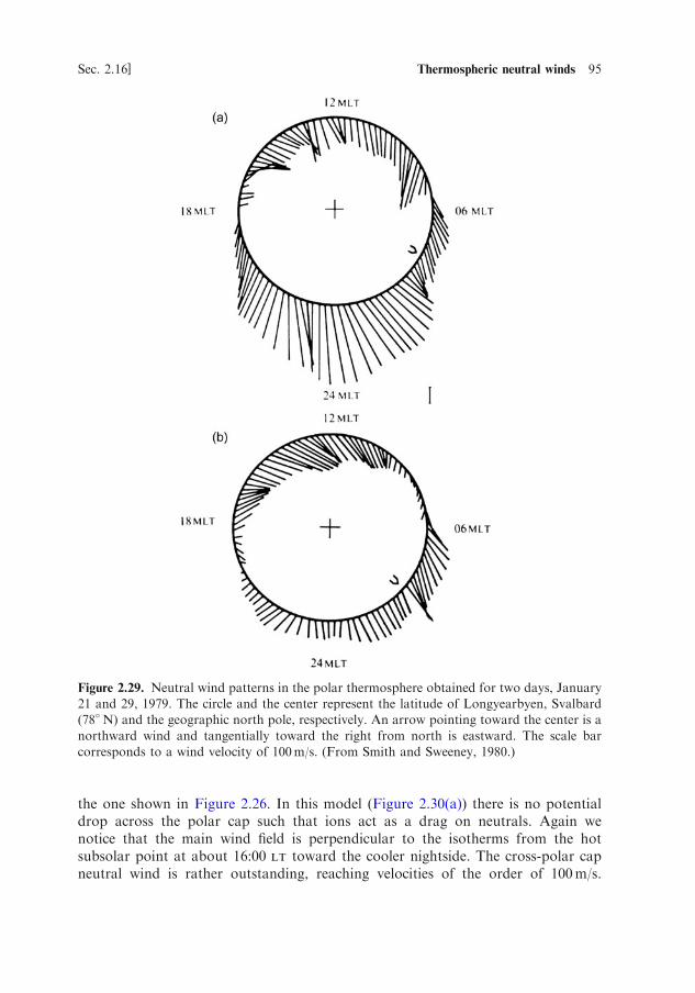
the one shown in Figure 2.26. In this model (Figure 2.30(a)) there is no potentialdrop across the polar cap such that ions act as a drag on neutrals. Again wenotice that the main wind field is perpendicular to the isotherms from the hotsubsolar point at about 16:00 lt toward the cooler nightside. The cross-polar capneutral wind is rather outstanding, reaching velocities of the order of 100m/s.
2.16 Thermospheric neutral winds 95]Sec. 2.16
Figure 2.29. Neutral wind patterns in the polar thermosphere obtained for two days, January
21 and 29, 1979. The circle and the center represent the latitude of Longyearbyen, Svalbard
(78� N) and the geographic north pole, respectively. An arrow pointing toward the center is a
northward wind and tangentially toward the right from north is eastward. The scale bar
corresponds to a wind velocity of 100m/s. (From Smith and Sweeney, 1980.)

When, however, a cross-polar cap potential of about 60 kV is applied (Figure2.30(b)), the wind field as well as the temperature distribution changes character;the latter is related to local heating due to enhanced collisions between theneutrals and ions (Joule heating). The velocities across the polar region arestrongly enhanced (notice the change in scales by a factor of more than 3 on thevelocity arrows). At night-time the high-latitude velocities are more stronglyequatorward related to the surge, as noticed already in relation to Figure 2.28. In
96 The atmosphere of the Earth [Ch. 2
Figure 2.30. (a) Calculated global circulation and temperatures along a constant pressure
surface corresponding to about 300 km for the case of solar heating as the only driving force
mechanism. The contours describe the temperature perturbation in K and the arrows give wind
directions. The length of the arrows gives the wind speed with a maximum of 100m/s. (b) The
same as in (a) except that a magnetospheric convection source with cross-tail potential corre-
sponding to 60 kV is included. The wind speed represented by the length of arrows now
corresponds to 336m/s. (From Dickinson et al., 1984.)

the daytime, however, at middle latitudes the velocities are strongly reduced andthe zonal component is reversed from eastward to westward. These effects are dueto enhanced Joule heating at high latitudes caused by strong currents in theauroral zone.
That electromagnetic disturbances at high latitudes can have a significanteffect at thermospheric heights is illustrated more clearly in Figure 2.31. In panel(a) the meridional circulation under quiet conditions is mainly forced by solarheating which produces a large cell with warm air rising at the equator, flowingtowards the poles, and sinking down again to lower heights. Above the polarregions (>70� latitude), however, a small cell with the opposite flow direction isset up above 300 km altitude due to heat influx from the magnetosphere outsidethe plasmapause. In panel (b), however, in which a large magnetic storm takesplace, the contrary cell expands in altitude (down to 120 km) as well as in latitude(down to the equator around 200 km of altitude). Air rich in molecular constitu-ents rises in the thermosphere above the high-latitude regions and is being broughtat high altitude toward the equator where the air descends to about 150 km. Ionswith high velocities are observed flowing outward from the thermosphere alongmagnetic field lines during such stormy events.
2.17 E-REGION WINDS
By now moving down in altitude to study E-region winds, it is again useful tocompare the different terms in the equation of motion (2.26). In Figure 2.32 theoutcome of such a comparison for the same high-latitude station as shown inFigure 2.27 is presented.
Contrary to the F-region situation where the pressure and ion drag termappeared to be dominant forcing mechanisms to the neutral wind, it is thepressure and Coriolis term that rule over the E-region neutral air motion. Aglobal model calculation of the E-region neutral wind at about 120 km of altitudeis illustrated in Figure 2.33(a) against isothermal contours. It is noticed that incontrast to F-region winds which are mainly directed perpendicularly to the iso-therms, the E-region neutral air motion more closely follows these contour lines.A geostrophic component is therefore present in E-region neutral winds. E-regionwind speeds are also only a third of F-region speeds on average. A 60 kV cross-polar cap potential is enforced on the ion motion for the wind data shown inFigure 2.33(b). The high-latitude winds are now predominantly eastward and thecross-polar cap motion is reduced. At low latitudes, however, there do not appearto be marked changes in the E-region wind field.
2.18 OBSERVATIONS OF E-REGION NEUTRAL WINDS
Due to the strong coupling between neutrals and ions in the E-region, observa-tions of the ion motion can sometimes be used as a tracer for the neutral motion.
2.18 Observations of E-region neutral winds 97]Sec. 2.18

Let us now consider the equation of motion for the ions (2.33). In the steady statewhen dvi=dt ¼ 0, we can solve for neutral velocity in a simple manner:
un ¼ vi �q
mivi;nvi � B� q
mivi;nE ð2:34Þ
At high latitude where the magnetic field is almost vertical, this equation appliesto the horizontal component of un while the vertical component is assumed equalto the ion motion along the magnetic field line. We notice that when in is verylarge, the neutral velocity is equal to the ion velocity. Observing the ion motionby some radio or radar technique therefore allows for deriving the neutral motion
98 The atmosphere of the Earth [Ch. 2
Figure 2.31. Calculated contours of a mass flow stream function. The numbers on the contours
are in g/s. The difference between the contour values gives the global flux mass between the two
contours. (a) For solar heating as the only driving source. (b) For solar heating, Joule heating
and momentum source also included. (From Dickinson et al., 1975.)

in a rather direct manner. For smaller values of in the complete coupling betweenions and neutrals as given by (2.34) has to be accounted for in order to derive unfrom measurements of vi. By means of an incoherent scatter radar such asEISCAT close to Tromsø, Norway (70� N) one can obtain almost simultaneousobservations of E- and F-region velocities. In the F-region (300 km) where the col-lision term will be negligible to the ion motion compared with the E-field andLorentz force term, the electric field can be derived for a steady-state solution(1.29):
E ¼ �vFi � B
where vFi is the F-region ion velocity observed simultaneously with the E-region
ion velocity. The neutral wind in the E-region can then be derived with anappropriate choice of collision frequency model.
Figure 2.34 illustrates neutral wind (x; y; z) components in the geographicalframe of reference as a function of time at several E-region heights for quiet days(Ap � 16) in the four seasons. From such time series the mean velocity compo-nents as well as the average 24-, 12-, 8-, and 6-hour tidal components can bederived for each of the six heights. This has been carried out for all four seasonsand the results are presented in Figure 2.35. The most outstanding feature of these
2.18 Observations of E-region neutral winds 99]Sec. 2.18
Figure 2.32. Similar to the data shown in Figure 2.27 but applied at 120 km approximately.
(From Killeen and Roble, 1986.)

components is the strong mean eastward wind between 90 and 120 km having amaximum at about 110 km of 60m/s in summer and 20m/s in winter. The verylow mean northward and vertical wind components in the same height region arealso noticeable; these components are relatively less influenced by change ofseason.
The eastward component of the diurnal tide increases gradually by height andreaches an amplitude close to 100m/s above 120 km. The northward component ofthis tide is fairly independent of height. For the other horizontal tidal componentsno systematic height dependence is found. In the vertical component, however, alltidal components except the 6-hour tide have a minimum amplitude at the height
100 The atmosphere of the Earth [Ch. 2
Figure 2.33. Same as for Figure 2.30 except that the constant pressure level corresponds to close
to 120 km. (a) The maximum wind speed corresponds to 32m/s. (b) The maximum wind speed
corresponds to 79m/s. (From Dickinson et al., 1984.)

region of the strong mean eastward wind. In Figure 2.36 wind components pre-sented as a function of time for the six E-region heights for quiet autumn days inFigure 2.34 are shown as horizontal clock dial plots. We notice the outstandingdaytime poleward wind at the four lower heights 96–117 km. Clearly, there arelarge variations by height in the neutral wind in the auroral E-region.
It is generally believed, in spite of the long time constants involved (as shownin Figure 2.23), that the E-region neutral velocities will be modified during strongauroral disturbances at the higher latitudes.
A similar averaging process of the average neutral wind at different E-regionheights has been performed on data obtained by EISCAT under disturbed con-ditions (Ap > 16). The mean velocity components as well as the tidal componentsare shown as a function of height in Figure 2.37. Data obtained from 11 disturbeddays are compared with corresponding data from 24 quiet days (Ap � 16). Wenotice that the strong eastward mean velocity is rather unaffected by the conditionof disturbance, and is more dependent on season (as shown in Figure 2.35). Anoutstanding feature in the auroral E-region is therefore an eastward neutral jetstream or superrotation. The most outstanding difference between quiet and dis-turbed days appears to be the enhancement of the eastward diurnal tide above110 km altitude.
By the EISCAT Svalbard Radar (ESR) it is also possible to derive theE-region neutral wind at polar latitudes. A comparison of the height profiles ofthe mean wind and diurnal and semidiurnal tides is shown in Figure 2.38 forobservations in Tromsø and Longyearbyen, Svalbard (78.1� N, 15.3� E). It isnoticed that the behavior of the different components is rather similar except thatthe mean eastward wind in Tromsø is weaker than in the polar cap latitude.
To study the importance of the electric field on the neutral wind at differentheights, Figure 2.39 shows a correlation analysis of the horizontal neutral windcomponents and the electric field at different altitudes as derived from Tromsøand Svalbard. It is noticed that the correlation coefficient is very low (�0) below110 km for all components and that the neutral wind appears to be less influencedby the E-field above 110 km in Longyearbyen than in Tromsø. The ion dragappears to be less efficient at higher latitudes. The eastward component of theneutral wind in Tromsø appears almost in antiphase with the electric field above120 km while the northward component has a maximum correlation for bothplaces at about 115 km.
2.19 VERTICAL MOTION
It is of special interest to study vertical winds, although these are usually verysmall compared with horizontal winds and also difficult to measure. They are,however, important as they play a significant role in the vertical transport ofmomentum and kinetic energy, and also of gravity potential energy. Furthermore,vertical winds control to a large extent the vertical distribution of the differentconstituents as we have seen in relation to diffusion. Let us assume that there are
2.19 Vertical motion 101]Sec. 2.19

102 The atmosphere of the Earth [Ch. 2

2.19 Vertical motion 103]Sec. 2.19
Figure
2.34.Theaverageneutralw
indcomponentsderived
bytheEISCATincoherentscatter
radaratTromsø
(69.66� N
,18.94� E
)atseven
E-
regionheightsforquietdays(A
p�
16)in
thefourseasons.Theseaveragewindcomponentsare
derived
byaddingthemeanwindcomponents
together
withthe24-,12-,8-,and6-hourtidalcomponents
withappropriate
phases.(C
ourtesyNozawa,1994.)

104 The atmosphere of the Earth [Ch. 2

2.19 Vertical motion 105]Sec. 2.19
Figure
2.35.(U
pper
row
ofpanels)
Themeancomponents
asafunctionofheightforthefourseasons.
(Fourlower
rowsofpanels)
The
24-,12-,8-,and6-hourtidalcomponents
asafunctionofheightforthefourseasons.(From
Brekkeet
al.,1994.)

106 The atmosphere of the Earth [Ch. 2
Figure 2.36. The average horizontal neutral wind velocity vectors at six different E-region
heights for the average quiet autumn day. These vectors are obtained by adding together
the appropriate north and east components in Figure 2.34. (From Brekke et al., 1994.)

no horizontal gradients in density but that the atmosphere is vertically stratifiedð@=@x ¼ @=@y ¼ 0Þ.
For a quasi-steady state ð@=@t ¼ 0Þ we derive from the continuity equation
d�
dtþ �r � u ¼ 0
@�
@tþ ðu � rÞ�þ �r � u ¼ 0
ðu � rÞ�þ �r � u ¼ 0
9>>>>>=>>>>>;ð2:35Þ
and
w@�
@zþ �r � u ¼ 0
where we have used u ¼ ðu; v;wÞ. By multiplying by p and dividing by � we get
pr � u ¼ � p
�
@�
@zw ð2:36Þ
From the equation of state for an ideal gas
p ¼ �RT ð2:37Þwhere R ¼ 8.3 J/molK is the individual gas constant, we form
@p
@z¼ R �
@T
@zþ T
@�
@z
� �and solving for @�=@z gives:
@�
@z¼ 1
T
1
R
@p
@z� �
@T
@z
� �By inserting this into (2.36) we have
pr � u ¼ � p
�
1
T
1
R
@p
@z� �
@T
@z
� �w ¼ � @p
@z� p
T
@T
@z
� �w
The vertical velocity is now given by
w ¼ � pr � u@p
@z� p
T
@T
@z
By introducing the partial derivative @T=@p and the barometric law (2.5) we have:
w ¼ pr � ug� 1� p
T
@T
@p
� � ð2:38Þ
The vertical velocity is now expressed by the divergence of u and the variation intemperature by pressure. By introducing the scale height from (2.6) into (2.38), we
2.19 Vertical motion 107]Sec. 2.19
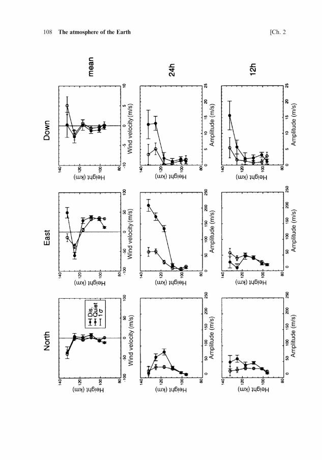
108 The atmosphere of the Earth [Ch. 2

2.19 Vertical motion 109]Sec. 2.19
Thestandard
deviationsare
shownbyverticalbars.(From
NozawaandBrekke,
1995.)
Figure
2.37.Thevariationwithheightofthenorthward,eastward,anddownward
componentsofthemeanwindandtheamplitudes
ofthe24-,
12-,8-,and6-hourtidalcomponents.Thedifferentdisturbance
levelsare
indicatedbyquiet(A
p�
16)anddisturbed
(Ap>
16)conditions.

110 The atmosphere of the Earth [Ch. 2
(a)

2.19 Vertical motion 111]Sec. 2.19
(b)
Figure 2.38. (a) Altitude profiles of mean wind (top), diurnal tidal amplitude (middle), and
semidiurnal amplitude (bottom) observed at Tromsø (circle) and Longyearbyen (triangle) are
presented for meridional (left) and zonal (right) components. For tidal components, larger filled
symbols denote data values whose significance level is greater than 90%, smaller filled symbols
whose significance level is between 90 and 50% and small open symbols denote data values
whose significance level is less than 50%. Horizontal lines associated with each symbol denote
error bars (1 standard deviation). (b) Corresponding phase values (in local time of maximum)
are shown for diurnal (top) and semidiurnal (bottom) components for meridional (left) and
zonal (right) components. (From Nozawa et al., 2005.)

have:
w ¼ Hr � u1� p
T
@T
@p
ð2:39Þ
For an isothermal atmosphere where @T ¼ 0 we find
w ¼ H@w
@zand
w ¼ w0 expz� z0H
� �when w ¼ w0 at a reference height z0. Vertical velocity therefore increases withheight for an expansion in an isothermal atmosphere. This comes about sincedensity decreases by height, and in order to keep the energy flux constant thevelocity must increase.
For an adiabatic expansion we get from (2.15)
p
T
@T
@p¼ � 1
and find from (2.39)
w ¼ H@w
@zand
w ¼ w�0 exp
z� z0H
� �
112 The atmosphere of the Earth [Ch. 2
Figure 2.39. Altitude profiles of correlation coefficients between the E-region neutral wind
components and the electric field as derived from Tromsø and Longyearbyen with incoherent
scatter observations. (Nozawa, private communication.)

Since > 1, the vertical velocity will increase more slowly with height in theadiabatic situation than for an expansion in an isothermal atmosphere.
The term pr � u represents a rate of mechanical work against the pressureforce due to expansion or compression. We now want to relate this to the changeof energy in the system.
The first law of thermodynamics per unit mass can be expressed by:
dq ¼ d"þ p
mdV ð2:40Þ
where q is the heat, d" ¼ cv dT is the change in the internal energy, and cv(¼ 712 JK�1 kg�1) is the heat capacity per unit mass at constant volume.
From the ideal gas law we have
p ¼ nkT ¼ �RT
and since
� ¼ m=V
dV ¼ �md�
�2
Inserting this into (2.40) and forming
_qq ¼ dq
dt
_qq ¼ _""� RT
�
d�
dt
Inserting from (2.35) for ð1=�Þðd�=dtÞ we have
_qq ¼ _""þ RTr � uAnd finally solving for r � u
r � u ¼ 1
RTð _qq� _""Þ
and multiplying by p we finally have
pr � u ¼ p
RTð _qq� _""Þ ¼ �ð _qq� _""Þ
The left-hand side represents the rate at which work is done by the system if theright-hand side is positive, and on the system if the right-hand side is negative.The vertical velocity can now be derived from (2.38):
w ¼ _qq� _""
g 1� p
T
@T
@p
� �
2.19 Vertical motion 113]Sec. 2.19

For an adiabatic process where _qq ¼ 0 we now have:
w ¼ � _""
g¼ � cv
gdT
dt
If the internal temperature increases with time, then work must be done on thesystem by the surroundings and the air must contract downward. In the oppositesense, if the temperature decreases, the work is done by the system and the atmo-sphere expands upward. Since we have only allowed for vertical motion, this isequivalent to considering the motion of a column of air in a cylinder with a fixedbase.
For external heat allowed to exchange with the system the situation can be farmore dramatic, especially if _qq is large. This occurs quite frequently within theauroral region of the upper atmosphere and then strong vertical motion can beexpected.
2.20 EXERCISES
1. Derive the total mass of an isothermal atmosphere and compare that with themass of the Earth.
2. Let the normalized velocity distribution in a gas in thermal equilibrium be givenby:
f ðvÞ ¼ 4 m
2 kT
� �3=2v2 exp � mv2
2kT
!
(a) Derive the average speed �vv.
(b) Show that the most probable speed
vm:p: ¼2kT
m
� �1=2
(c) Show that the root mean square speed
vr:m:s: ¼3kT
m
� �1=2
3. Choose a place in the atmosphere at latitude �. In a Cartesian coordinate systemx is positive eastward, y northward, and z in the vertical direction.
(a) Find the horizontal geostrophic wind components u and v in this coordinatesystem.
Let the pressure gradient around the equator look like that in Figure 2.40.
114 The atmosphere of the Earth [Ch. 2

(b) Give the zonal wind directions in the northern and southern hemisphere.
(c) Does it make sense to talk about a geostrophic wind at the equator?
Let the pressure gradient around the equator look like that in Figure 2.41.
(d) What do the zonal wind directions look like in both hemispheres in this case?
2.20 Exercises 115]Sec. 2.20
Figure 2.40
Figure 2.41