NBER WORKING PAPER SERIES

PHYSICIAN BELIEFS AND PATIENT PREFERENCES:A NEW LOOK AT REGIONAL VARIATION IN HEALTH CARE SPENDING

David CutlerJonathan SkinnerAriel Dora SternDavid Wennberg

Working Paper 19320http://www.nber.org/papers/w19320

NATIONAL BUREAU OF ECONOMIC RESEARCH1050 Massachusetts Avenue

Cambridge, MA 02138August 2013

Comments by Amitabh Chandra, Elliott Fisher, Mike Geruso, Tom McGuire, Nancy Morden, AllisonRosen, Gregg Roth, Pascal St.-Amour, Victor Fuchs, and seminar participants at the NBER SummerInstitute, Tinbergen Institute, Cornell, Tilburg, Erasmus, Lausanne, and Harvard Universities, CRISPHealth Econometrics, the Universities of Venice and Texas, and NBER’s Health Care Program Meeting,were exceedingly helpful. We are grateful to F. Jack Fowler and Patricia Gallagher of the Universityof Massachusetts Boston for developing the patient and physician questionnaires. Funding from theNational Institute on Aging (T32-AG000186-23 and P01-AG031098 to the National Bureau of EconomicResearch and P01-AG019783 to Dartmouth) and the Laboratory for Economic Applications and Policy(LEAP) at Harvard University (to Skinner) is gratefully acknowledged. Skinner is an investor in DorsataInc., a software company developing physician decision tools; Wennberg receives royalties from HealthDialog, a care management company, and owns stock in RxAnte, a drug compliance segmentationcompany. Survey data are available at www.intensity.dartmouth.edu. The views expressed herein arethose of the authors and do not necessarily reflect the views of the National Bureau of Economic Research.

At least one co-author has disclosed a financial relationship of potential relevance for this research.Further information is available online at http://www.nber.org/papers/w19320.ack

NBER working papers are circulated for discussion and comment purposes. They have not been peer-reviewed or been subject to the review by the NBER Board of Directors that accompanies officialNBER publications.

© 2013 by David Cutler, Jonathan Skinner, Ariel Dora Stern, and David Wennberg. All rights reserved.Short sections of text, not to exceed two paragraphs, may be quoted without explicit permission providedthat full credit, including © notice, is given to the source.

Physician Beliefs and Patient Preferences: A New Look at Regional Variation in Health CareSpendingDavid Cutler, Jonathan Skinner, Ariel Dora Stern, and David WennbergNBER Working Paper No. 19320August 2013JEL No. H51,I1,I11,I18

ABSTRACT

There is considerable controversy about the causes of regional variations in healthcare expenditures.We use vignettes from patient and physician surveys, linked to Medicare expenditures at the levelof the Hospital Referral Region, to test whether patient demand-side factors, or physician supply-sidefactors, explains regional variations in Medicare spending. We find patient demand is relatively unimportantin explaining variations. Physician organizational factors (such as peer effects) matter, but the singlemost important factor is physician beliefs about treatment: 36 percent of end-of-life spending, and17 percent of U.S. health care spending, are associated with physician beliefs unsupported by clinicalevidence.

David CutlerDepartment of EconomicsHarvard University1875 Cambridge StreetCambridge, MA 02138and NBERdcutler@harvard.edu

Jonathan SkinnerDepartment of Economics6106 Rockefeller HallDartmouth CollegeHanover, NH 03755and NBERjonathan.skinner@dartmouth.edu

Ariel Dora SternKennedy School of Government79 John F. Kennedy StCambridge, MA 02138arieldorastern@fas.harvard.edu

David WennbergGeisel School of Medicine35 Centerra ParkwayLebanon, NH 03766david.e.wennberg@dartmouth.edu

1

Regional variations in rates of medical treatments are large in the United States and other

countries (Skinner et al., 2012). For example, in the U.S. Medicare population over age 65,

price-adjusted per-patient Medicare expenditures ranged from under $7,000 to nearly $14,000,

with most of the variation unexplained by regional differences in patient illness or poverty.

What drives such variation in treatment and spending? One possibility is patient demand.

Many studies of variations have been conducted in environments where all patients have a

similar and fairly generous insurance policy,1 so price and income differences are unlikely to be

large. Still, heterogeneity in patient preferences for care may play a role. In very acute

situations, some patients may prefer to try all possible measures, while others may prefer

palliation and an out-of-hospital death. If patients with similar preferences group together

geographically – for example, if people who value life-prolonging treatments live in areas with

world-class interventional physicians – patient preference heterogeneity could lead to regional

variation in equilibrium outcomes (Anthony et al., 2010; Mandelblatt et al., 2012;).

Another possible source of variation arises from the supply side. “Supplier-induced

demand” describes a situation in which a health care provider shifts a patient’s demand curve

beyond what the patient would want. This would be true in a principle-agent framework

(McGuire and Pauly, 1991), if prices are high enough (and income scarce). While physician

utilization has been shown to be sensitive to prices (Jacobson et al., 2006, Clemens and Gottlieb,

2012), it would be difficult to explain observed Medicare variations using profit margins alone,

since reimbursement rates are set administratively and do not vary greatly across areas.

Variation in desired supply may also result from non-monetary incentives. Physicians

could respond to organizational pressure or peer pressure to perform more procedures, even if 1 This is generally true in the U.S. Medicare program. The presence of supplemental insurance coverage differs across the country, but most studies do not find that these differences affect utilization by more than a small degree (McClellan and Skinner, 2006).

2

their current income is no higher as a consequence. Physicians might also have differing beliefs

about appropriate treatments, particularly for conditions where there are few professional

guidelines (Wennberg et al., 1982). These differences in beliefs may arise because of differences

in where physicians received medical training (Epstein and Nicholson, 2009) or their personal

experiences with different treatments (Levine-Taub et al., 2011). If this variation is correlated

spatially – for example, if intensive physicians are more likely to hire physicians with similar

views – the resulting regional differences in beliefs could explain regional variations in

equilibrium spending.

It has proven difficult to estimate separately the impact of physician beliefs, patient

preferences, and other factors as they affect equilibrium healthcare outcomes, largely because of

challenges in identifying factors that affect only supply or demand (Dranove and Wehner, 1994).

We address this problem using “strategic surveys,” as in Ameriks et al. (2011), in which we use

survey vignettes to elicit motivation and clinical beliefs of physicians (suppliers), and attitudes

and preferences of patients (demanders) as well as intervention-specific preferences from both

groups. These responses are then linked to utilization measures at the regional level, which

allows us to estimate directly how supply and demand factors affect regional healthcare

utilization.

Patient preferences are measured by a survey of Medicare enrollees age 65 and older

asking about whether they would want a variety of aggressive care interventions. We focus on

the tradeoff between invasive procedures with potential longevity benefits versus palliative care

and comfort at the end of life. Physician beliefs are captured by two surveys, one of

cardiologists and the second of primary care physicians. Both sets of physicians were presented

with vignettes about four elderly individuals with chronic health conditions, and asked how they

3

would manage each one. Based on their responses, we characterize physicians along two non-

exclusive dimensions: those who consistently and unambiguously recommended intensive care

beyond guidelines (“cowboys”), and those who consistently recommended palliative care for the

very severely ill (“comforters”).

We first use these surveys to examine whether patient or physician preferences are more

important in explaining regional variations in care. Our results show that physician preferences

are significantly greater than patient preferences in explaining regional utilization patterns. In

some models, we can explain over half of the variation in end-of-life spending across areas by

knowing only how a small sample of physicians in an area would treat hypothetical patients. In

contrast, patient preferences explain little of the cross-area variation.

We then try to understand why physicians have the treatment preferences they do,

relating physicians’ views about optimal treatment to questions about malpractice concerns,

financial arrangements (fraction of Medicaid and capitated patients), and perceived

organizational pressures (providing treatment for patients who expected but didn’t need it, or

doing a procedure because the referring physician expected it). We find that only a fraction of

physicians claim to have made recent decisions as a result of purely financial considerations. We

also find that “pressure to accommodate” either patients (by providing treatments that are not

needed) or referring physicians (doing procedures to keep them happy and meet their

expectations) have a modest but significant relationship with physician beliefs about appropriate

care. While many physicians report making interventions as a result of malpractice concerns,

these responses do not explain the residual variation in treatment recommendations.

Ultimately, the largest degree of regional variation appears to be due to differences in

physician beliefs about the efficacy of particular therapies. Physicians in our data have starkly

4

different views about how to treat the same patients, and these views are not highly correlated

with demographics, background, and practice characteristics, and are often not consistent with

professional guidelines for appropriate care. As much as 36 percent of end-of-life Medicare

expenditures, and 17 percent of overall Medicare expenditures, are explained by physician

beliefs that cannot be justified either by patient preferences or by clinical effectiveness.

I. A Model of Variation in Utilization

We develop a simple model of patient demand and physician supply. The demand side of

the model is a standard one; the patient’s indirect utility function is a function of out-of-pocket

prices (p), income (Y), and preferences for care (η); V = V(p, Y, η). Solving this for optimal

intensity of care, x, yields xD. As in McGuire (2011), we assume that xD is the fully informed

patient’s demand for the quantity of procedures prior to any demand “inducement.”

On the supply side, we assume that physicians seek to maximize the perceived health of

their patient, s(x), by appropriate choice of inputs x, subject to patient demand (xD), financial

considerations, and organizational factors. Note that the function s(x) captures both patient

survival and quality of life, for example as measured by quality-adjusted life years (QALYs).

Individual physicians are assumed to be price-takers (after their networks have negotiated

prices with insurance companies), but face a wide range of reimbursement rates from private

insurance providers, Medicare, and Medicaid. The model is therefore simpler than models in

which hospital groups and physicians jointly determine quantity, quality, and price, (Pauly,

1980) or where physicians exercise market power over patients to provide them with “too much”

health care (McGuire, 2011). Following Chandra and Skinner (2012), we write the physician’s

overall utility as:

(1) 𝑈 = Ψ𝑠(𝑥) + Ω(𝑊 + 𝜋𝑥 − 𝑅) −𝜙(|𝑥 − 𝑥𝐷|) − 𝜑(|𝑥 − 𝑥𝑂|)

5

where Ψ is perceived social value of improving health, Ω is the physician’s utility function of

own income, comprising her fixed payment W (a salary, for example) net of fixed costs R, and

including the incremental “profits” from each additional test or procedure performed, π.2 The

sign of π depends on the type of procedure and the payment system a physician faces.

The third term represents the loss in provider utility arising from the deviation between

the quantity of services the provider recommends (x) and what the informed patient demands

(xD). This function could reflect classic supplier-induced demand – from the physician’s point of

view, xD is too low relative to the physician’s optimal x – or it may reflect the extent to which

physicians are acting as the agent of the (possibly misinformed) patient, for example when the

patient wants a procedure that the physician does not feel is medically appropriate. The fourth

term reflects a parallel influence on physician decision making from organizational factors that

do not directly affect financial rewards, such as (physician) peer pressure.

The first-order condition for (1) is:

(2) Ψ𝑠′(𝑥) = −Ω′𝜋 + 𝜙′ + 𝜑′ ≡ 𝜆

Physicians provide care up to the point where the choice of x reflects a balance between the

perceived marginal value of health, Ψs′(x), and factors summarized by λ: (a) the incremental

change in net income π, weighted by the importance of financial resources Ω′, (b) the

incremental disutility from moving patient demand away from where it was originally, 𝜙′, and

(c) the incremental disutility from how much the physician’s own choice of x deviates from her

organization’s perceived optimal level of intervention, 𝜑′.

2 We ignore capacity constraints, such as the supply of hospital or ICU beds.

6

In this model,3 there are two ways to define “supplier-induced demand.” The broadest

definition is simply the presence of any equilibrium quantity of care beyond the level of the ex

ante preferences of an informed patient, i.e. x > xD. This is still relatively benign; the marginal

value of this care may still be positive. More relevant is the sign of s(x) - s(xD); does the

additional care enhance or diminish health outcomes? Supplier-induced demand could more

narrowly be defined as s(x) - s(xD ) ≤ 0; patients gain no improvement in health outcomes and

may even experience a decline in health or a significant financial loss. Note that both of these

definitions leave the question of physician knowledge of inducement undefined. That is, a

physician with strong (but incorrect) beliefs may over-treat her patients, even in the absence of

financial or organizational incentives to do so.

To develop an empirical model, we adopt a simple closed-form solution of the utility

function for physician i:4

(1′) 𝑈𝑖 = Ψ𝑠𝑖(𝑥𝑖) + 𝜔[𝑊𝑖 + 𝜋𝑖𝑥𝑖 − 𝑅𝑖] −𝜙2

(𝑥𝑖 − 𝑥𝑖𝐷)2 – 𝜑2

(𝑥𝑖 − 𝑥𝑖𝑂�2

Note that ω/Ψ reflects the relative tradeoff between the physician’s income and the value of

improving patient lives, and thus might be viewed as a measure of “professionalism.” The first-

order condition is therefore:

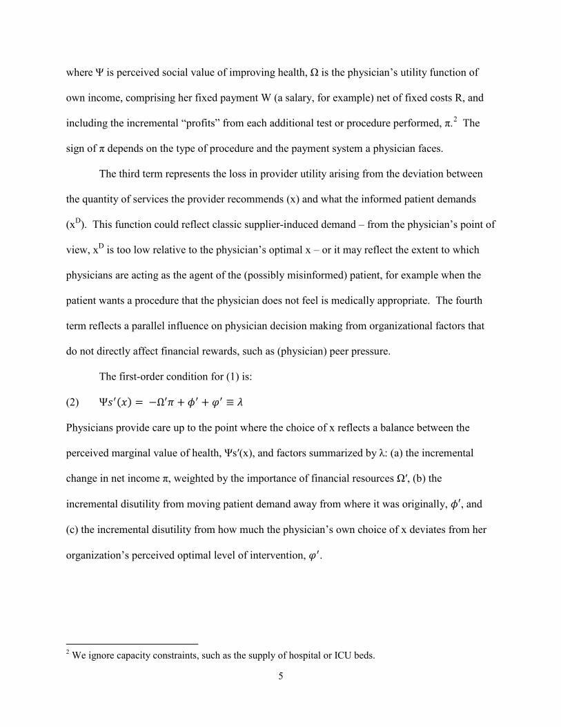
(2′) Ψ𝑠𝑖′(𝑥𝑖) = 𝜆 ≡ −𝜔𝜋𝑖 + 𝜙(𝑥𝑖 − 𝑥𝑖𝐷) + 𝜑(𝑥 − 𝑥𝑖𝑂)

Figure 1 shows Ψs'(x) and λ. Note that λ is linear in x with an intercept equal to −(𝜔𝜋𝑖 +

𝜙𝑥𝑖𝐷 + 𝜑𝑥𝑖𝑂). Note also the key assumption that patients are sorted in order from most

appropriate to least appropriate for treatment, thus describing a downward sloping Ψs'(x) curve.

The equilibrium is where Ψs'(x) = λ, at point A. A shift in the intercept, which depends on

3 A more general model would account for the patient’s ability to leave the physician and seek care from a different physician, as in McGuire (2011). 4 We are grateful to Pascal St.-Amour for suggesting this approach.

7

reimbursement rates for procedures π, taste for income ω, regional demand xD, and

organizational or peer effects xO, would yield a different λ*, and hence a different utilization

rate. But all of these factors affect the intensity of treatments via a movement along the marginal

benefit curve, Ψs′(x).

Alternatively, it may be that si′(x) differs across physicians – productivity differs, rather

than constraints. For example, if si′(x) = αi s′(x), where s′(x) is average physician productivity

and α varies across regions, this would be represented as a shift in the marginal benefit curve.

Point C in Figure 1 corresponds to greater intensity of care than point A and arises naturally

when the physician is or believes she is more productive. For example, heart attack patients

experience better outcomes from cardiac interventions in regions with higher rates of

revascularization, consistent with a Roy model of occupational sorting (Chandra and Staiger,

2007). Because patients in regions with high intervention rates benefit differentially from these

interventions, this scenario does not correspond to the narrow definition of “supplier-induced

demand.”

The productivity shifter α may also vary because of “professional uncertainty” – a

situation where the physician’s perceived α differs from the true α (Wennberg et al., 1982). For

example, physicians may be overly optimistic with respect to their ability to perform procedures,

leading to expected benefits that exceed actual realized benefits. Baumann et al. (1991) have

documented the phenomenon of “macro uncertainty, micro certainty” in which physicians and

nurses are sure that their treatment benefited a specific patient (micro certainty) even when there

is no general consensus on which procedure is more clinically effective (macro uncertainty).

8

Much of the evidence from psychology5 argues for overconfidence in one’s own ability, leading

to a natural bias towards doing more.

To see this in Figure 1, suppose the actual benefit is s′(x) but the perceived benefit is

g′(x). The equilibrium is point C; the incremental treatment harms the patient, even though the

physician believes the opposite. In equilibrium, this supplier behavior would appear consistent

with classic supplier-induced demand, but the cause is quite different.

Empirical Specification. To examine these theories empirically, we consider variation in

practice at the regional level (for reasons explained below). Taking a first-order Taylor-series

approximation of equation (2′) for region i yields a linear equation that groups equilibrium

outcomes into two components, demand factors ZD and supply factors ZS:

(4) 𝑥𝑖 = �̅� + 𝑍𝑖𝐷 + 𝑍𝑖𝑆 + 𝜀𝑖.

The demand-side component is:

(5) 𝑍𝑖𝐷 = 𝜙M

(𝑥𝑖𝐷 − �̅�𝐷)

where 𝑀 = −Ψ𝑠"(�̅�) + 𝜙 + 𝜑. This first element of equation (5) reflects the higher average

demand for health care, multiplied by the extent to which physicians accommodate that demand,

ϕ. The supply side component is:

(6) 𝑍𝑖𝑆 = 1𝑀

{ωΔ𝜋𝑖 + πΔ𝜔𝑖 + 𝜙(𝑥𝑖𝑂 − �̅�𝑂) + Ψ𝑠′(�̅�)Δ𝛼𝑖}

The first term in equation (6) reflects how differences in profits in region i relative to the national

average (Δπ) affect utilization. The second term reflects the extent to which physicians weight

income more heavily. The third term captures organizational goals in region i relative to national

5 If the patient gets better, the physician gets the credit, but if the patient gets worse, the physician is able to say that she did everything possible (Ransohoff et al., 2002).

9

averages (𝑥𝑖𝑂 − �̅�𝑂). The final term captures the impact of different physician beliefs about

productivity of the treatment (Δ𝛼𝑖); this term shifts the marginal productivity curve.6

Equation (4) can be expanded to capture varying parameter values as well – for example,

in some regions physicians may be more responsive to patient demand (a larger ϕi). These

interactive effects, considered below, reflect the interaction of supply and demand and would

magnify the responses here.

II. Data and Estimation Strategy

In general, it is difficult to distinguish among demand and supply explanations for

treatment variation; even detailed clinical data reveal only a subset of what the physician knows.

Further, patient preferences and physician beliefs about the desirability or appropriateness of

different procedures are unknown in ex post clinical data. In studying motives for household

saving, Ameriks et al. (2011) implemented “strategic surveys” to identify demand and supply.

We follow this approach here, using surveys asking potential patients about preferences for

hypothetical end-of-life choices (that is, xD before their interaction with the physician), and

asking physicians how they would treat a set of hypothetical patients with varying disease

severity, as well as questions about their financial and organizational constraints.

In an ideal world, patient surveys would be matched with surveys from their treating

physicians. Because our data do not match physicians with their own patients, we instead

matched supply and demand at the area level by HRR, or Hospital Referral Region.7 In equation

(4), we therefore define x to be a regional average spending measure. Our primary measure is the

natural logarithm of risk-adjusted and price-adjusted Medicare expenditures in the last two years 6 Note that these effects are scaled by 1/M, which depends on –s″. If returns to treatment do not decline rapidly, strongly-held physician opinions can lead to highly variable treatment rates (Chandra and Skinner, 2012). 7 These HRRs are defined in the Dartmouth Atlas of Health Care, which divides the United States into 306 HRRs. Spending measures are based on area of residence, not where treatment is actually received.

10

of life. We also consider several other measures such as one-year risk- and price-adjusted

expenditures for Medicare enrollees for hip fracture, and overall price-adjusted Medicare

expenditures.

Our first estimation, based on Equation 4, asks whether area-level supply or demand

factors can better explain actual regional expenditures. Our second estimates then seeks to

understand why physicians hold the beliefs they do (Equation 6). For the latter, we relate

individual physician vignette responses to financial and organizational factors. We interpret

vignette responses that cannot be explained by demographic, organizational or financial

incentives as reflecting primary physician beliefs (e.g., a shift in perceived marginal treatment

curve from Ψs′(x) to Ψg′(x)). We describe each survey in turn.

Patient Survey. The survey sampling frame was all Medicare beneficiaries in the 20%

denominator file who were age 65 or older on July 1, 2003 (Barnato et al., 2009). A random

sample of 4,000 individuals was drawn; the response rate was 65%. We limited the final sample

to respondents who provided all variables of interest, leaving a total of 1,413 Medicare

beneficiary surveys. The final sample of respondents reside in 64 of the larger HRRs, all of

which have sufficient physician observations to be included in the empirical model.

We used responses to 5 survey questions, with the exact wording shown in Panel I of

Appendix A. Since the questions patients respond to are hypothetical and typically describe

scenarios that have not yet happened, we think of them as xD, or preferences not affected by

physician advice.

11

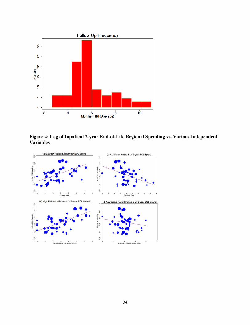
Two of the questions relate to unnecessary care, asking people if they would like a test or

cardiac referral even if their primary care physician did not think they needed one (Table 1).8

Overall, 73 percent of patients wanted such a test and 56 percent wanted a cardiac referral.

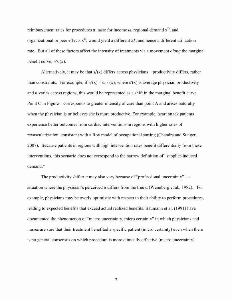
There is wide variation across regions in averages responses to these question. Figure 2 shows

the distribution of the share of patients responding that they wanted an unnecessary specialist

referral for the 64 larger HRRs; the standard deviation of the area average is 10 percent. While

some of this variation is likely due to small sample sizes within HRRs, we tested for the null of

no regional variation by bootstrapping the distribution of area spending assuming people were

randomly assigned to areas; p–values are reported in the last column of Table 1.

The three other questions, grouped into two binary indicators, measured preferences for

end-of-life care. One reflected patients’ desire for aggressive care at the end of life: whether

they respond that they would want to be put on a respirator if it would extend their life for either

a week (one question) or a month (another question). The second question asked, if the patient

reached a point at which they were feeling bad all of the time, would they want drugs to make

them feel better, even if those drugs might shorten their life. In each case, there is statistically

significant variation across areas (Table 1).

Patients’ preferences are generally positively correlated across items. For example, the

correlation coefficient between wanting an unneeded cardiac referral and wanting an

unnecessary test is 0.43 (p < .01). But other comparisons point to very modest associations, for

example a -0.02 correlation coefficient between wanting palliative care and wanting to be on a

respirator at the end of life.

8 This question captures pure patient demand independent of what the physician wants. Note, however, that patients could still answer they would not seek an additional referral if they were unwilling to disagree with their physician.

12

Since survey responses may vary systematically by demographic covariates such as race

and ethnicity; we create demographically-adjusted HRR-level measures of preferences by

adjusting for observed patient characteristics (race, age and sex).

Physician Surveys. A total of 999 cardiologists were randomly selected to receive the

survey. Of these, 614 cardiologists responded, for a response rate of 61%. Seventeen physicians

did not self-identify as cardiologists, and 88 physicians were missing crucial information such as

practice type or practiced in HRRs with too few respondents to include in the analysis, leaving us

a final sample of 509 cardiologists. These cardiologists practice in 64 HRRs, all of which have 3

or more cardiologists represented in the survey.

The primary care physician (PCP) responses come from a parallel survey of PCPs (family

practice, internal medicine, or internal medicine/family practice). A total of 1,333 primary care

physicians were randomly selected to receive the survey. The response rate was 73%. A total of

840 PCPs had complete responses to the survey and practiced in HRRs with enough local

respondents to include in the analysis.

Physicians were asked about a number of clinical vignettes, discussed in the next section,

as well as a variety of characteristics of their practices. Two measures of financial circumstances

are reported in Table 1 for all physicians: the share of patients for whom they are reimbursed on

a capitated basis (on average, 16 percent), and the share of a physician’s patients on Medicaid

(10 percent), with both factors generally associated with lower marginal reimbursement.

A second set of questions asks about characteristics of the physician and her practice.

Twenty-nine percent are in small practices, 60 percent are in single or multi-specialty group

practices, and 11 percent are in HMOs or hospital-based practices. We also observe a number of

13

characteristics about the physician, including age, gender, whether the physician is board

certified, and the number of weekly patient days practiced.

Third, the survey asks about physician’s actual responsiveness to external incentives over

the past year, including how frequently, if ever, in the past 12 months they have intervened for

non-clinical reasons. We create a set of binary variables that indicates whether a physician

responded to each set of incentives at least “sometimes” (i.e. “sometimes” or “frequently”) over

the past year. Ten percent of cardiologists reported that they had sometimes or frequently

performed a cardiac catheterization because of the expectations of the referring physician; 41

percent of all physicians did so because of colleague’s expectations (Table 1).

Medicare Utilization Data. We match the survey responses with expenditure data by

HRR. Our primary measure is Medicare expenditures in the last two years of life for enrollees

over age 65 with a number of fatal illnesses.9 All HRR-level measures are adjusted for age, sex,

race, differences in Medicare reimbursement rates and the type of disease (including an indicator

for multiple diseases). This measure implicitly adjusts for differences across regions in health

status; an individual with renal failure who subsequently dies is likely to be in similar (poor)

health regardless of whether she lives in West Virginia or Oregon.10 End-of-life measures are

commonly used to instrument for health care intensity, (e.g., Fisher et al., 2003), are highly

correlated with other medical expenditure measures such as one-year expenditures following a

heart attack (Skinner et al., 2010), and do not appear sensitive to the inclusion of additional

individual-level risk-adjusters (Kelley, et al., 2012). In sensitivity analysis, we consider price-

9 These include congestive heart failure, cancer/leukemia, chronic pulmonary disease, coronary artery disease, peripheral vascular disease, severe chronic liver disease, diabetes with end organ damage, chronic renal failure, and dementia. 10 If more intensive spending saves lives, then in regions with more intensive spending, fewer die, leading to potential biases in the end-of-life measure (Bach et al., 2004). However, the bias can be either positive or negative, and, given conventional estimates of cost-effectiveness in end-of-life spending, the magnitude of the bias would be small.

14

adjusted Medicare expenditures for all fee-for-service enrollees age 65 and above, and a

“forward looking” measure of one-year expenditures following hospital admission for a different

severe condition, hip fracture. The HRR-level price-adjusted expenditures for the hip fracture

cohort are adjusted for age, sex, race, comorbid conditions at admission, and the hierarchical

condition categories (HCC) risk-adjustment index for the 6 months prior to admission. We focus

on the 64 HRRs in the combined sample with a minimum of 3 cardiologists (average =5.4) and 2

primary care physicians (average = 7.9) surveyed. Among patients, we observe an average of 22

respondents per HRR.

III. Clinical Vignettes from the Physician Surveys

Since the clinical vignettes are crucial for our analysis, we describe them in some detail.

We note first the obvious: responses to the vignette may not be what physicians would actually

do in practice. Empirical evidence, however, strongly indicates that clinical vignettes closely

predict how physicians intervene (Peabody et al., 2004; Mandelblatt et al., 2012; Dresselhaus et

al., 2004).

We assume that the physician’s responses to the vignettes are “all in” measures (ZS, as in

equation 6), reflecting physician beliefs as well as the variety of financial, organizational, and

capacity-related constraints physicians face. Alternatively, one could interpret the physician’s

responses to the vignettes as a pure reflection of beliefs (for example, how one might answer for

qualifying boards), and not as representative of the day-to-day realities of their practice. We

tested this alternative explanation by including the organizational and financial variables in our

estimation equations in addition to the vignette estimates. This did not appreciably increase the

explanatory power of these equations.

15

One might alternatively argue that physicians in regions where most of their low-income

patients are in poor health may “fill in” missing characteristics of the vignettes, and be more

likely to recommend intensive care. Thus imperfectly risk-adjusted Medicare expenditures would

be spuriously correlated with more intensive vignette recommendations. However, such

physicians may be less likely to recommend intensive medical or surgical treatments, since

outcomes are dependent on coordinated follow-up care that may not be available to patients

living in low-income neighborhoods.

The detailed clinical vignette questions are in Appendix A (Panel II); summary statistics

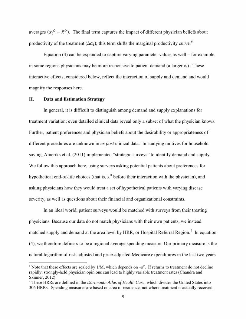
are presented in Table 1. We begin with the vignette for Patient A, which asks how frequently

the physician would schedule routine follow-up visits for patients with stable angina whose

symptoms and cardiac risk factors are now well controlled on current medical therapy

(cardiologists) or patients with hypertension (primary care physicians). The response is

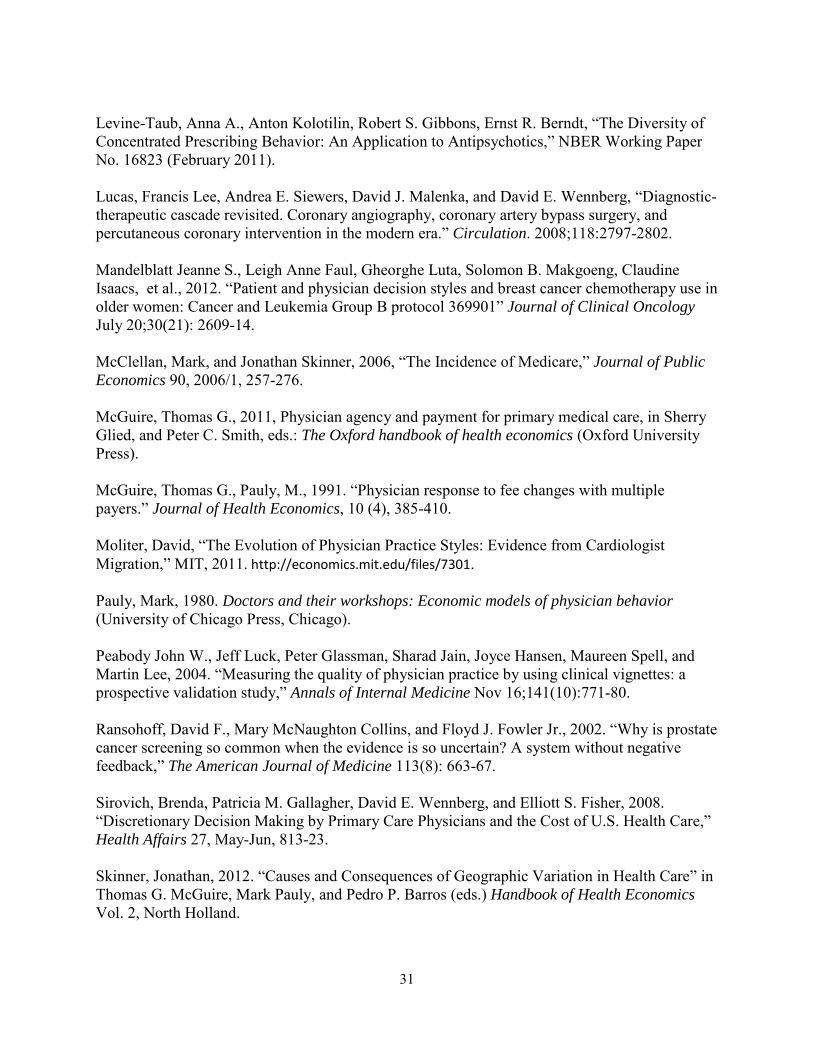
unbounded, and expressed in months, which in practice ranged from 1 month to 24 months.

Figure 3 presents a HRR-level histogram of averages from the cardiology survey for all regions

with at least 3 cardiologists.

How do these responses correspond to guidelines for managing chronic stable angina?

While diagnosis and management of coronary artery disease (the cause of angina) is the most

common clinical issue faced by cardiologists on a day-to-day basis, there are no hard data to

support any recommendation. The 2005 American College of Cardiology/American Heart

Association [ACC/AHA] guidelines (Hunt et al., 2005) – what most cardiologists would have

considered the “Bible” in the field at the time the survey was fielded – were very imprecise: they

recommended follow-up every 4-12 months. However, even with these broad recommendations,

16

we find that over one fifth (23%) of cardiologists in the sample recommend follow-up visits

more frequently than every 4 months.

The equivalent follow-up measure for primary care physicians is for a patient with well-

controlled hypertension. The Seventh Report of the Joint National Committee on Prevention,

Detection, Evaluation, and Treatment of High Blood Pressure (U.S. Department of Health and

Human Services, 2004), which would have been the most current guideline recommendation at

the time, suggests follow up every 3-6 months based on expert opinion.

We define a “high follow up” physician as one who recommends follow-up visits more

frequently than clinical guidelines would suggest and a “low follow up” physician as one who

recommends follow-up visits less frequently than clinical guidelines would suggest. By this

definition, fewer than 1 percent of cardiologists and 9 percent of PCPs in our data are classified

as “low follow-up” physicians while 23 percent of cardiologists and 9 percent of PCPs are

classified as “high follow-up” physicians.

Office visits are not a large component of physicians’ income (or overall Medicare

expenditures). Thus any correlation between the frequency of follow-up visits and overall

expenditures would most likely be because frequent office visits are also associated with more

highly remunerated tests and interventions (such as echocardiography, stress imaging studies,

and so forth) that further set in motion the “diagnostic-therapeutic cascade,” resulting in

subsequent diagnostic tests, treatments, and follow-up visits (Lucas, et al., 2008). Thus the next

two vignettes focus on patients with heart failure, a much more expensive setting. Heart failure is

also natural to ask about because it is common, the disease is chronic, prognosis is poor, and

treatment is expensive.

17

Vignettes for Patients B and C ask questions about the treatment of Class IV heart failure,

the most severe classification and one in which patients have symptoms at rest. In both scenarios

the patient is on maximal (presumably optimal) medications, and neither is a candidate for

revascularization: Patient B already had a coronary stent placed without symptom change, and

Patient C is explicitly noted to not be a candidate for this procedure. The key differences

between the two scenarios are patients’ ages (75 in the first, 85 in the second), the presence of

asymptomatic non-sustained ventricular tachycardia in the younger man, and severe symptoms

that resolve partially with increased oxygen in the older man.

Cardiologists in the survey were asked about various interventions as well as palliative

care for each of these patients. For patient B, they were given five choices: three intensive

treatments (repeat angiography; implantable cardiac defibrillator [ICD], and pacemaker

insertion), one involving medication (anti arrhythmic therapy), and palliative care. Patient C also

has three intensive options (admit to the ICU/CCU, placement of a coronary artery catheter, and

pacemaker insertion), two less aggressive options (admit to the hospital (but not the ICU/CCU)

for diuresis, and send home on increased oxygen and diuresis) and palliative care. In each case,

cardiologists ranked their likelihood of recommending each intervention individually on a range

from “never” to “always / almost always.” Physicians could indicate strong or weak support for

more than one option, for example, for both palliative care and an intervention.

We start with the obvious: regardless of the religious, political or moral persuasion of the

cardiologist, these two men deserve a frank conversation about their prognosis and an

ascertainment of their preferences for end-of-life care. One-year mortality for those with Class

IV heart failure is nearly 50 percent. If compliant with the guidelines, therefore, every one of the

18

cardiologists should have answered “always/almost always”, or at least “most of the time,” to

initiating or continuing discussions about palliative care.11

Studies have shown that patients, physicians and family members are often not on the

“same page” when it comes to advanced directive planning (Connors, et al., 1995), and this

shows up in the data. For Patient B, only 30 percent of cardiologists responded that they would

take this course of action “most of the time” or “always/almost always.” For Patient C, 43

percent of cardiologists and 50 percent of primary care physicians were likely to recommend this

course of action most of the time or always/almost always. In both cases, physicians’

recommendations fall short of clinical guidelines. We define our second index of physicians to

reflect this. We classify the doctor as a “comforter” if the physician would discuss palliative

care with the patient “always / almost always” for both Patients B and C (cardiologists) or just

for patient C (primary care physicians). In our final sample, 29 percent of cardiologists and 44

percent of primary care physicians met the requirement for being a comforter.

We now turn to more controversial aspects of patient management. The language in the

vignettes was carefully constructed relative to the contemp-oraneous guidelines. Several key

aspects of Patient B rule out both the ICD and pacemaker insertion12 and indeed the ACC-AHA

guidelines explicitly recommend against the use of an ICD for Class IV patients potentially near

death (Hunt et al., 2005; p. e206). On the other hand, both treatments are highly reimbursed.

Since patient C is already on maximal medications and is not a candidate for

revascularization, the management goal should be to make him as comfortable as possible. This

11 According to the AHA-ACC directives, “Patient and family education about options for formulating and implementing advance directives and the role of palliative and hospice care services with reevaluation for changing clinical status is recommended for patients with HF [heart failure] at the end of life.” (Hunt et al., 2005, p. e206) 12 This includes his advanced stage; his severe (Class IV) medication refractory heart failure; and the asymptomatic non-sustained nature of the ventricular tachycardia.

19

goal should be accomplished in the least invasive manner possible (e.g., at home), and if that is

not possible in an uncomplicated setting, for example during admission to the hospital for simple

diuresis. According to the ACC/AHA guidelines, no additional interventions are appropriate.13

In fact, even a “simple” but invasive test, the pulmonary artery catheter, has been found to be of

no marginal value over good clinical decision making in managing patients with CHF, and could

even cause harm (ESCAPE, 2005).

Despite these guideline recommendations, physicians in our data show a surprising

degree of enthusiasm for additional interventions. For patient B, nearly one-third of the

cardiologists surveyed would recommend a repeat angiography some of the time, most of the

time, almost always, and always. Similarly, 65 percent of cardiologists recommend an ICD most

of the time, always or almost always, while 47 percent recommend a pacemaker. For patient C,

18 percent recommend an ICU/CCU admission, 2 percent recommend a pulmonary artery

catheter and 15 percent recommend a pacemaker at least most of the time.

Our next measure of ZS is based on a summary of these intensity recommendations. We

start with the three most intensive interventions for both patients. Cardiologists’ responses on

aggressiveness are highly correlated across these two patients. Of the 28 percent (N=143) of

cardiologists in the sample who would “frequently” or “always/almost always” recommend at

least one of the above-listed high-intensity procedures for patient C, 93 percent (N=133) would

also frequently or always/almost always recommend at least one high-intensity intervention for

patient B. We use this overlap (the highest treatment recommendation overlap in our data) to

define a “cowboy” cardiologist – a cardiologist who recommends at least one of the three

possible intensive treatments to both patients B and C most of the time or always/almost always.

13 Clinical improvement with a simple intervention (increasing his oxygen) also argues against more intensive interventions.

20

Because Vignette B was not presented to the primary care physicians, we use only their response

to Vignette C to categorize them using the same criteria. In total, 27 percent of the cardiologists

in our sample are classified as cowboys, as are 19 percent of the primary care physicians.

All told, we test four measures of ZS: high or low frequency of follow-up visits, a dummy

variable for being a cowboy, and a dummy variable for being a comforter. How are these

measures related? Table 2 shows that among both PCPs and cardiologists, chi-squared tests

strongly reject the null of no association between follow-up frequencies recommended for

vignette patients and status as a “cowboy” or “comforter.” Physicians with a low follow-up

frequency are more likely to be comforters and less likely to be cowboys than physicians with a

high follow-up frequency. Similarly, cowboy physicians are far less likely to be comforter

physicians (even though doctors could be classified as both). Most differences are statistically

significant.

IV. Model Estimates

We now proceed with our estimates of the models presented above. We first consider

Equation (4), the relationship between area-level spending and local patient and physician

preferences. We then turn to Equation (6), modeling the factors leading physicians to be more

and less aggressive.

Do Survey Responses Predict Regional Medicare Expenditures?

We start with the basic relationship between area spending, patient preferences and

physician preferences for the 64 HRRs with at least 3 cardiologists and 2 primary care physician

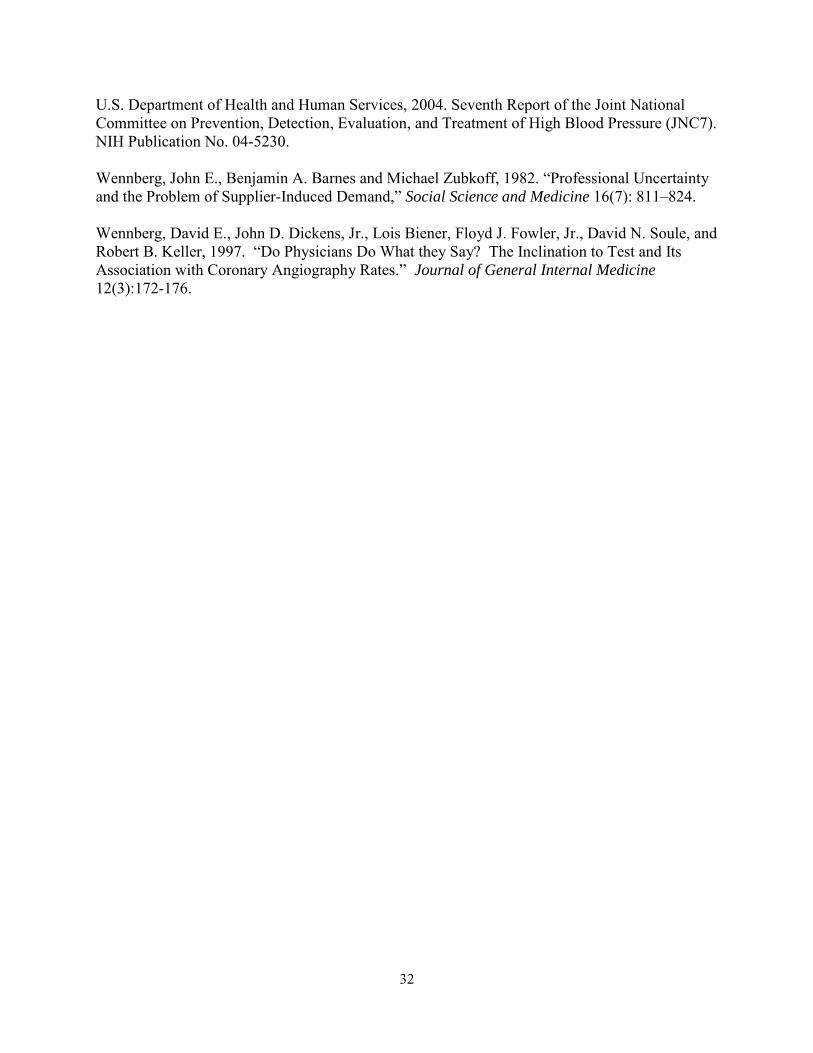
responses. Figure 4 shows scatter plots between area-level end of life spending and our

measures of supply and demand for care. The measures we include are the fraction of all

physicians in the area who are cowboys (panel a), the fraction of physicians who are comforters

21

(panel b), the fraction of physicians who recommend follow-up more frequently than

recommended guidelines (panel c), and the share of patients who desire more aggressive care at

the end of life (panel d). Each circle is an HRR, and the size of the circle is proportional to the

respective survey sample size in the HRR.

In the case of the three supply-side variables, the results are consistent with the theory:

despite the small sample sizes of physicians per HRR, end of life spending is positively related to

the cowboy ratio, negatively related to the comforter ratio, and positively related to high

frequency of follow-up visits. The demand variable, in contrast, is not related to spending; the

data points form a cloud more than a line.

Table 3 explores this result more formally with regression estimates of log end-of-life

expenditures, weighted by the number of physician observations per HRR and including controls

for the fraction of PCPs among our survey responders. As the first column shows, the local

proportion of cowboys and comforters predicts 36 percent of the observed regional variation in

risk-adjusted end-of-life spending. Further, the estimated magnitudes are large: increasing the

percentage of cowboys by 10 percentage points increases end-of-life expenditures by 7.5 percent,

while increasing the fraction of comforters by 10 percent reduces expenditures by 4.1 percent.

This relationship between spending and the local fractions of cowboys and comforters holds for

both cardiologists and primary care physicians analyzed separately, as shown in the Appendix.

Column 2 of Table 3 shows that the indicator for high frequency follow-up

recommendations is also a meaningful predictor of HRR-level end-of-life spending; conditional

on the fraction of cowboys and comforters, an increase of 10 percentage points in the percentage

of physicians who prefer to see patients more frequently than guidelines recommend is predicted

to increase end-of-life spending by 9.5 percent; and while the low follow-up coefficient is large

22

in magnitude (-0.417), it is not statistically significant. The combination of just these supplier

beliefs alone explains over 60 percent of the observed end-of-life spending variation in the 64

HRRs observed.14

The next two columns add measures of patient preferences to the regressions: the share of

patients wishing to have unneeded tests, the share wanting to see an unneeded cardiologist, the

share preferring aggressive end-of-life care, and the share preferring comfortable end-of-life

care. None of these variables are statistically significant at the 5% level. Even excluding the

physician belief variables entirely, as in column 6, the R2 from the patient preference variables is

just 0.075. Separate regressions for cardiologists and primary care physicians are presented in

Appendices C and D and indicate similar results.15

It is possible that there is an interaction effect between patient preferences and physician

beliefs, for example if aggressive physicians interact with aggressive patients to generate even

more utilization (or conversely for comforter physicians and patients). These hypotheses are

considered in Table 4. Column 1 of the table repeats Column 5 of Table 3 for reference. The

subsequent columns add interaction terms. As shown in Column 2, however, there is little

consistent evidence for the interactive aggressiveness hypothesis; the interaction between

cowboy physicians and patients with aggressive preferences is negative (not positive as theory

would suggest), and while the coefficient between comforter physicians and patients is negative

(column 3), it is not significant.

Column 4 of Table 4 repeats the analyses in column 1, but uses total average per

beneficiary expenditures (adjusted for prices, age, sex, and race/ethnicity) as the dependent 14 As Black et al. (2000) note, the OLS estimate is a lower bound and under weak assumptions, the expected value of the OLS parameter estimate is of smaller magnitude than the true parameter. (The R2 is also a lower bound owing to measurement error.) 15 Our results do not appear to be driven by geography. The coefficient estimates are similar when the east and west coasts of the US are estimated separately.

23

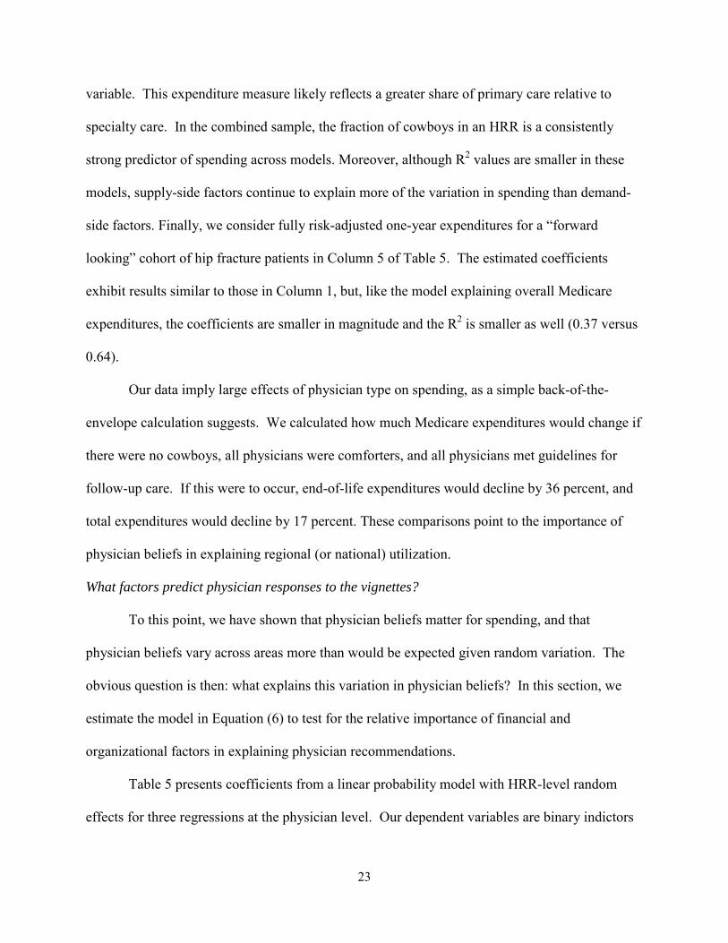
variable. This expenditure measure likely reflects a greater share of primary care relative to

specialty care. In the combined sample, the fraction of cowboys in an HRR is a consistently

strong predictor of spending across models. Moreover, although R2 values are smaller in these

models, supply-side factors continue to explain more of the variation in spending than demand-

side factors. Finally, we consider fully risk-adjusted one-year expenditures for a “forward

looking” cohort of hip fracture patients in Column 5 of Table 5. The estimated coefficients

exhibit results similar to those in Column 1, but, like the model explaining overall Medicare

expenditures, the coefficients are smaller in magnitude and the R2 is smaller as well (0.37 versus

0.64).

Our data imply large effects of physician type on spending, as a simple back-of-the-

envelope calculation suggests. We calculated how much Medicare expenditures would change if

there were no cowboys, all physicians were comforters, and all physicians met guidelines for

follow-up care. If this were to occur, end-of-life expenditures would decline by 36 percent, and

total expenditures would decline by 17 percent. These comparisons point to the importance of

physician beliefs in explaining regional (or national) utilization.

What factors predict physician responses to the vignettes?

To this point, we have shown that physician beliefs matter for spending, and that

physician beliefs vary across areas more than would be expected given random variation. The

obvious question is then: what explains this variation in physician beliefs? In this section, we

estimate the model in Equation (6) to test for the relative importance of financial and

organizational factors in explaining physician recommendations.

Table 5 presents coefficients from a linear probability model with HRR-level random

effects for three regressions at the physician level. Our dependent variables are binary indictors

24

for whether the physician is a cowboy (Column 1), a comforter (Column 2), or believes in high

follow-up (Column 3). In each model, we include basic physician demographics: age, gender,

board certification status, whether the physician is a cardiologist, and days per week spent seeing

patients, as well as cardiologists per 100,000 Medicare beneficiaries.

The demographic factors reveal that older physicians are more likely to recommend high

rates of follow-up and are more likely to be cowboys, but age is not a significant predictor of

comforter status. Male physicians are less likely to be comforters, while board certification – a

marker for physician quality – is negatively associated with cowboy status and high follow-up

frequency. This result is consistent with Doyle et al. (2010), who found that lower quality

physicians spent 10-25% more for otherwise identical patients.

A greater number of cardiologists per 100,000 Medicare beneficiaries is associated with a

higher likelihood of a physician being a cowboy or high follow-up doctor and with a lower

likelihood of the physician being a comforter. One might be tempted to interpret this as classic

“supplier-induced demand” effect, with more cardiologists per capita leading to less income per

cardiologist, and hence a greater incentive to treat a given patient more intensively. Yet the

equilibrium supply of cardiologists is likely to depend on a wide variety of factors, suggesting

caution in the interpretation.

The substitution effect implies that lower incremental reimbursements associated with

Medicaid and capitated patients would lead to fewer interventions and more palliative care.

Table 5 shows that physicians with a larger fraction of Medicaid and (to a lesser extent) capitated

patients are more likely to be cowboys and high-follow-up physicians, rejecting the substitution

hypothesis. One may appeal again to a strong income effect to explain these patterns.

25

Some organizational factors are strongly associated with physician beliefs about

appropriate practice. Physicians in solo or 2-person practices are far more likely to be aggressive

than physicians in single or multi-specialty group practices or physicians who are part of an

HMO or a hospital-based practice. Yet physicians in group or staff model HMOs or hospital-

based practices are no more likely to be comforters. Physicians who respond to patient

expectations are predicted to be comforters, and those responding to referring physician

expectations are more likely to be high follow-up physicians, but neither effect is significant.

Whether cardiologists accommodate referring physicians – a financial factor (since cardiologists

will benefit financially from future referrals) as well as an organizational one – is a large and

significant predictor of being a cowboy.16 Finally, malpractice concerns are not predictive of

cowboy or comforter status, perhaps because procedures performed on high-risk patients (such

as Patients B and C) can increase the risk of a malpractice suit.

The explanatory power of these regressions is quite modest – between 6 and 15 percent –

suggesting that a considerable degree of the remaining variation is the consequence of physician

beliefs regarding the productivity of treatments, rather than behavior caused by financial,

organizational, or other factors.

As a final exercise, we include these financial, organizational, and responsiveness

variables, aggregated up to the HRR, in a regression that seeks to explain the variation in log

end-of-life spending – an expanded counterpart to Table 4. These results are presented in

Appendix E. Aside from the per-capita supply of cardiologists – a potentially suspect measure of

capacity – none of the additional variables are significant, nor do they add appreciably to the

explanatory power of the regression. Physician beliefs independent of financial or organizational

16 Note that this question is asked only of cardiologists.

26

factors appear to explain why physicians are cowboys or comforters (or both) and how that

affects overall spending.

V. Conclusion and Implications

While there is a good deal of regional variation in medical spending and care utilization

in the U.S. and elsewhere, there is little agreement about the causes of such variations. Do they

arise from variation in patient demand, from variation in physician behavior, or both? In this

paper, we found that patient demand as measured by responses to a nationwide survey has

modest predictive association with regional end-of-life expenditures. By contrast, individual

physician beliefs regarding treatment options can explain a substantial degree of regional

variation in utilization among the U.S. Medicare population. While other results have suggested

such a finding (Sirovich et al. (2008), Lucas et al. (2008), Bederman et. al. (2011), and

Wennberg et al. (1997)), our paper is the first to directly relate Medicare spending to physician

beliefs. The regressions imply that, were physicians to follow professional guidelines, end-of-

life Medicare expenditures would be 36 percent less, and overall expenditures 17 percent lower.

We then turned to the factors that lead physicians to have different preferences. We

found that the traditional factors in supplier-induced demand models, such as the fraction of

patients paid through capitation (or on Medicaid), or the responsiveness to financial factors, play

a relatively small role in explaining equilibrium variations in utilization patterns. Organizational

factors such as accommodating colleagues help to explain some, but not most, individual

intervention decisions. Instead, differences in physician beliefs about the effectiveness of

treatments are the primary source of variation in Medicare expenditures.17

17 This result is consistent with Epstein and Nicholson (2009), who find large variations in Cesarean section surgical rates among obstetricians within the same practice, even after adjusting for where the physicians trained.

27

Our results differ from the existing literature in that they are based on vignettes and thus

represent a lower bound to practice variations. Generally, prior studies inferred practice

variations as the residual from an area model, leading to estimates being biased either upward

(because of unobserved regional factors) or biased downward (because of flawed risk-

adjustment, as in Song et al., 2010).

One concern about the interpretation of the vignette responses as “overuse” is that they

may reflect the true productivity of physicians. While we cannot rule this out, we note that

physicians with greater objective qualifications such as board certification are no more likely to

be cowboys. Nor do the updated 2009 heart failure guidelines recommend more aggressive care

(Hunt et al., 2009), as a model of inappropriately cautious and slowly evolving recommendations

would suggest.

Another hypothesis is that while “cowboys” may over-treat patients along some

dimensions, they may also avoid the underuse of effective care along other dimensions (e.g.,

Landrum et al., 2008). Our survey did not ask about whether the physician provides effective

care or not. But other evidence does not support this hypothesis: an HRR-level composite AMI

quality measure from 2007 Hospital Compare data, (Dartmouth Atlas, 2013) is negatively

associated with the HRR-level fraction of physicians who are cowboys.

We know little about how physician beliefs arise. Simple heterogeneity in physician

beliefs cannot explain regional variation in expenditures, since regional patterns of beliefs

exhibit greater variation than would be expected due to chance alone. Rather, spatial correlation

in beliefs is required in order to explain the regional patterns we see. We do find that physicians’

propensity to intervene for non-clinical reasons is related to the expectations of physicians with

whom they regularly interact, a result consistent with network models. Similarly, Molitor (2011)

28

finds that cardiologists who move to more or less aggressive regions change their practice style

to better conform to local norms. But we are still left with questions as to how and why some

regions become more aggressive than others.

Our results do not imply that economic incentives are unimportant. Clearly, changes in

payment margins have a large impact on behavior, as has been shown in a variety of settings.

But the prevalence of geographic variations in European countries, where economic incentives

are often blunted, is consistent with the view that physician beliefs play a large role in explaining

such variations. A better understanding of both how physician beliefs form, and (if necessary)

how they can be shaped, is a key challenge for future research.

29

References Ameriks, John, Andrew Caplin, Steven Laufer, and Stijn van Nieuwerburgh, 2011. “The Joy of Giving or Assisted Living? Using Strategic Surveys to Separate Public Care Aversion from Bequest Motives,” Journal of Finance, 66(2) (April), 519-561. Anthony, Denise L., M. Brooke Herndon, Patricia M. Gallagher, Amber E. Barnato, Julie P.W. Bynum, et al., 2009. “How Much do Patients' Preferences Contribute to Resource Use?” Health Affairs 28, May-Jun, 864-73. Bach, Peter B., Deborah Schrag, and Colin B. Begg, 2004. “Resurrecting Treatment Histories of Dead Patients: A Study Design That Should Be Laid to Rest,” JAMA 292(22) (December 8): 2765-2770. Barnato, Amber E., M. Brooke Herndon, Denise L. Anthony, Patricia Gallagher, Jonathan S. Skinner, et al., 2007. “Are regional variations in end-of-life care intensity explained by patient preferences? A study of the US Medicare population,” Medical Care 45, 386-393. Baumann, Andrea O., Raisa B. Deber, Gail G. Thompson, 1991, “Overconfidence Among Physicians and Nurses: The ‘Micro-Certainty, Macro-Uncertainty’ Phenomenon,” Social Science and Medicine 32(1): 167-74. Bederman S. Samuel, Peter C. Coyte, Hans J. Kreder, Nizar N. Mahomed, Warren J. McIsaac, and James G. Wright, 2011. “Who’s in the driver's seat? The influence of patient and physician enthusiasm on regional variation in degenerative lumbar spinal surgery: a population-based study,” Spine; 36(6): 481-489. Black, Dan A.; Mark C. Berger; Frank A. Scott, 2000. “Bounding Parameter Estimates with Nonclassical Measurement Error,” Journal of the American Statistical Association, Vol. 95, No. 451, pp. 739-748. Chandra, Amitabh, and Douglas O. Staiger. 2007. “Productivity Spillovers in Healthcare: Evidence from the Treatment of Heart Attacks,” Journal of Political Economy 115, 103-140. Chandra, Amitabh, and Jonathan Skinner, 2012, “Productivity growth and expenditure growth in U.S. Health care,” Journal of Economic Literature 50(3) (September): 645-80. Clemens, Jeffrey, and Joshua Gottlieb, 2012. “Do Physicians' Financial Incentives Affect Medical Treatment and Patient Health?” Stanford University (SIEPR), http://siepr.stanford.edu/publicationsprofile/2447. Connors Alfred F., Jr, Neal V. Dawson, Normal A. Desbiens, et al. 1995: “A Controlled Trial to Improve Care for Seriously III Hospitalized Patients: The Study to Understand Prognoses and Preferences for Outcomes and Risks of Treatments (SUPPORT).” JAMA. 274(20):1591-1598. Dartmouth Atlas, 2013. http://www.dartmouthatlas.org/tools/downloads.aspx

30

Doyle, Joseph, Steven Ewer, and Todd Wagner, 2010. “Returns to Physician Human Capital: Evidence from Patients Randomized to Physician Teams” Journal of Health Economics. 29(6). December 2010: 866-882. Dranove, David, and Paul Wehner, 1994. “Physician-induced demand for childbirths,” Journal of Health Economics 13(1) (March): 61–73. Dresselhaus, Timothy R., John W. Peabody, Jeff Luck, Dan Bertenthal, 2004. “An Evaluation of Vignettes for Predicting Variation in the Quality of Preventive Care,” Journal of General Internal Medicine, October; 19(10): 1013–1018. Epstein, Andrew J., and Sean Nicholson, 2009. "The formation and evolution of physician treatment styles: An application to cesarean sections," Journal of Health Economics, 28(6) (December): 1126-1140. (ESCAPE) Evaluation Study of Congestive Heart Failure and Pulmonary Artery Catheterization Effectiveness: The ESCAPE Trial. JAMA. 2005; 294(13): 1625-1633. Fisher, Elliott S., David E. Wennberg, Terese A. Stukel, Daniel J. Gottlieb, Francis Lee Lucas, et al., 2003, “The implications of regional variations in Medicare spending. Part 2: Health outcomes and satisfaction with care,” Ann Intern Med 138, Feb 18, 288-98. Gruber, Jonathan, and Maria Owings. 1996. Physician financial incentives and cesarean section delivery. Rand Journal of Economics 27 (1):99-123. Hunt, Sharon Ann, William T. Abraham, Marshall H. Chin, Arthur M. Feldman, Gary S. Francis, et al., 2005. “ACC/AHA 2005 Guideline Update for the Diagnosis and Management of Chronic Heart Failure in the Adult,” Circulation. 2005;112:e154-e235; (September 13). Hunt, Sharon Ann, William T. Abraham, Marshall H. Chin, Arthur M. Feldman, Gary S. Francis, et al., 2009. “2009 Focused Update Incorporated Into the ACC/AHA 2005 Guidelines for the Diagnosis and Management of Chronic Heart Failure in the Adult,” Circulation 119:e391-e479 (March 26). Jacobson, Mireille, A. James O’Malley, Craig C. Earle, Juliana Pakes, Peter Gaccione and Joseph P. Newhouse, 2006. “Does Reimbursement Influence Chemotherapy Treatment For Cancer Patients?” Health Affairs, 25(2): 437-443. Kelly, Amy S., Susan L. Ettner, Sean Morrison, Qingling Du, Neil S. Wenger, and Catherine A. Sarkislan, 2011. “Determinants of Medical Expenditures in the Last 6 Months of Life,” Annals of Internal Medicine 154:235-242. Landrum, Mary Beth, Ellen R. Meara, Amitabh Chandra, Edward Guadagnoli and Nancy L. Keating, 2008. “Is Spending More Always Wasteful? The Appropriateness of Care and Outcomes among Colorectal Cancer Patients,” Health Affairs 27(1):159-168 (January).

31

Levine-Taub, Anna A., Anton Kolotilin, Robert S. Gibbons, Ernst R. Berndt, “The Diversity of Concentrated Prescribing Behavior: An Application to Antipsychotics,” NBER Working Paper No. 16823 (February 2011). Lucas, Francis Lee, Andrea E. Siewers, David J. Malenka, and David E. Wennberg, “Diagnostic-therapeutic cascade revisited. Coronary angiography, coronary artery bypass surgery, and percutaneous coronary intervention in the modern era.” Circulation. 2008;118:2797-2802. Mandelblatt Jeanne S., Leigh Anne Faul, Gheorghe Luta, Solomon B. Makgoeng, Claudine Isaacs, et al., 2012. “Patient and physician decision styles and breast cancer chemotherapy use in older women: Cancer and Leukemia Group B protocol 369901” Journal of Clinical Oncology July 20;30(21): 2609-14. McClellan, Mark, and Jonathan Skinner, 2006, “The Incidence of Medicare,” Journal of Public Economics 90, 2006/1, 257-276. McGuire, Thomas G., 2011, Physician agency and payment for primary medical care, in Sherry Glied, and Peter C. Smith, eds.: The Oxford handbook of health economics (Oxford University Press). McGuire, Thomas G., Pauly, M., 1991. “Physician response to fee changes with multiple payers.” Journal of Health Economics, 10 (4), 385-410. Moliter, David, “The Evolution of Physician Practice Styles: Evidence from Cardiologist Migration,” MIT, 2011. http://economics.mit.edu/files/7301. Pauly, Mark, 1980. Doctors and their workshops: Economic models of physician behavior (University of Chicago Press, Chicago). Peabody John W., Jeff Luck, Peter Glassman, Sharad Jain, Joyce Hansen, Maureen Spell, and Martin Lee, 2004. “Measuring the quality of physician practice by using clinical vignettes: a prospective validation study,” Annals of Internal Medicine Nov 16;141(10):771-80. Ransohoff, David F., Mary McNaughton Collins, and Floyd J. Fowler Jr., 2002. “Why is prostate cancer screening so common when the evidence is so uncertain? A system without negative feedback,” The American Journal of Medicine 113(8): 663-67. Sirovich, Brenda, Patricia M. Gallagher, David E. Wennberg, and Elliott S. Fisher, 2008. “Discretionary Decision Making by Primary Care Physicians and the Cost of U.S. Health Care,” Health Affairs 27, May-Jun, 813-23. Skinner, Jonathan, 2012. “Causes and Consequences of Geographic Variation in Health Care” in Thomas G. McGuire, Mark Pauly, and Pedro P. Barros (eds.) Handbook of Health Economics Vol. 2, North Holland.

32

U.S. Department of Health and Human Services, 2004. Seventh Report of the Joint National Committee on Prevention, Detection, Evaluation, and Treatment of High Blood Pressure (JNC7). NIH Publication No. 04-5230. Wennberg, John E., Benjamin A. Barnes and Michael Zubkoff, 1982. “Professional Uncertainty and the Problem of Supplier-Induced Demand,” Social Science and Medicine 16(7): 811–824. Wennberg, David E., John D. Dickens, Jr., Lois Biener, Floyd J. Fowler, Jr., David N. Soule, and Robert B. Keller, 1997. “Do Physicians Do What they Say? The Inclination to Test and Its Association with Coronary Angiography Rates.” Journal of General Internal Medicine 12(3):172-176.

33

Figure 1: Variations in Equilibrium: Differences in λ and Differences in Actual or Perceived Productivity

Figure 2: Fraction of Patients Who Would See Unneeded Cardiologist (HRR-Level Distribution)

Figure 3: Distribution of Length of Time before Next Visit for Patient with Well-Controlled Angina (Cardiologist HRR-Level Distribution)

34

Figure 4: Log of Inpatient 2-year End-of-Life Regional Spending vs. Various Independent Variables

Table 1: Primary Variables and Sample Distribution

Variable Mean Individual SD Area Average SD p-valueSpending and Utilization2-Year End-of-Life Spending $56,219 - $10,715 -6-Month End-of-Life Spending $14,272 - $2,660 -Total Per Patient Spending $7,837 - $1,032 -Hip Fracture Patient Spending $52,574 - $4,996 -Patient VariablesHave Unneeded Tests 73% 44% 10% <0.01See Unneeded Cardiologist 56% 50% 10% <0.01Aggressive Patient Preferences Ratio 8% 27% 5% <0.01Comfort Patient Preferences Ratio 48% 50% 12% <0.01Primary Care Physician VariablesCowboy Ratio 19% 39% 19% <0.01Comforter Ratio 44% 50% 20% <0.01Follow-Up Low 9% 28% 11% <0.01Follow-Up High 4% 19% 7% <0.01Cardiologist variablesCowboy Ratio 27% 45% 19% <0.01Comforter Ratio 29% 45% 20% <0.01Follow-Up Low 0% 4% 3% 0.09Follow-Up High 23% 44% 21% <0.01Organizational and Financial VariablesFraction Capitated Patients 16% 25% - -Fraction Medicaid Patients 10% 13% - -Weekly Patient Days 3.1 1.5 - -Physician Age 57.5 9.8 - -Board Certified 89% 31% - -Cardiologists per 100k 6.7 1.90 - -Responds to Referrer Expectations 10% 30% - -Responds to Colleague Expectations 41% 49% - -Responds to Patient Expectations 59% 49% - -Responds to Malpractice Concerns 43% 49% - -Responds to Practice Financial Incentives 32% 46% - -Note: The table shows means for the sample living or practicing in one of the 64 HRRs with at least 3cardiologists and 2 primary care physicians. The area average standard deviation is weighted by the numberof observations in the HRR. The p-value in the last column is for the null hypothesis of no excess varianceacross areas. The p-value is taken from a bootstrap of patient or physician responses across areas. For eachof 1,000 simulations, we draw patients or providers randomly (with replacement) and calculate the simulatedarea average and the standard deviation of that area average. The empirical distribution of the standarddeviation of the area average is used to form the p-value for the actual area average.

35

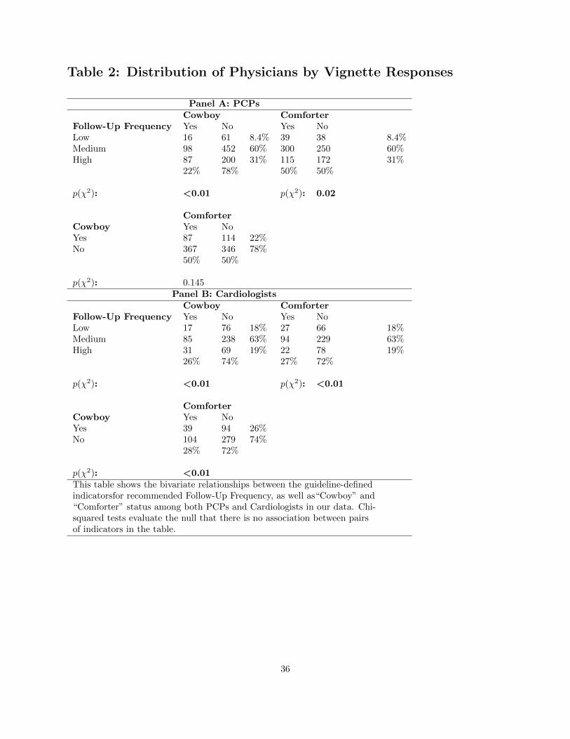
Table 2: Distribution of Physicians by Vignette Responses

Panel A: PCPsCowboy Comforter

Follow-Up Frequency Yes No Yes NoLow 16 61 8.4% 39 38 8.4%Medium 98 452 60% 300 250 60%High 87 200 31% 115 172 31%

22% 78% 50% 50%

p(χ2): <0.01 p(χ2): 0.02

ComforterCowboy Yes NoYes 87 114 22%No 367 346 78%

50% 50%

p(χ2): 0.145Panel B: Cardiologists

Cowboy ComforterFollow-Up Frequency Yes No Yes NoLow 17 76 18% 27 66 18%Medium 85 238 63% 94 229 63%High 31 69 19% 22 78 19%

26% 74% 27% 72%

p(χ2): <0.01 p(χ2): <0.01

ComforterCowboy Yes NoYes 39 94 26%No 104 279 74%

28% 72%

p(χ2): <0.01This table shows the bivariate relationships between the guideline-definedindicatorsfor recommended Follow-Up Frequency, as well as“Cowboy” and“Comforter” status among both PCPs and Cardiologists in our data. Chi-squared tests evaluate the null that there is no association between pairsof indicators in the table.

36

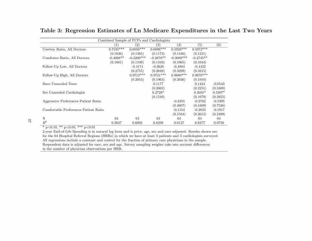
Table 3: Regression Estimates of Ln Medicare Expenditures in the Last Two Years

Combined Sample of PCPs and Cardiologists

(1) (2) (3) (4) (5) (6)

Cowboy Ratio, All Doctors 0.7535*** 0.6056*** 0.6096*** 0.5928*** 0.5972***(0.1626) (0.1385) (0.1173) (0.1446) (0.1221)

Comforter Ratio, All Doctors -0.4068** -0.3206*** -0.2878** -0.3089*** -0.2745**(0.1681) (0.1109) (0.1103) (0.1065) (0.1044)

Follow-Up Low, All Doctors -0.4174 -0.3626 -0.4884 -0.4422(0.2755) (0.2849) (0.3299) (0.3215)

Follow-Up High, All Doctors 0.9712*** 0.9721*** 0.9680*** 0.9670***(0.2053) (0.1963) (0.2026) (0.1910)

Have Unneeded Tests 0.1177 0.1424 -0.0543(0.2062) (0.2251) (0.3400)

See Unneeded Cardiologist 0.2728* 0.3035* 0.5397*(0.1549) (0.1679) (0.2855)

Aggressive Preferences Patient Ratio -0.2355 -0.2762 -0.5395(0.4607) (0.4409) (0.7526)

Comfortable Preferences Patient Ratio -0.1154 -0.2033 -0.1917(0.1584) (0.2015) (0.2499)

N 64 64 64 64 64 64R2 0.3627 0.6092 0.6299 0.6127 0.6377 0.0750

* p<0.10, ** p<0.05, *** p<0.012-year End-of-Life Spending is in natural log form and is price, age, sex and race adjusted. Results shown arefor the 64 Hospital Referral Regions (HRRs) in which we have at least 3 patients and 3 cardiologists surveyed.All regressions include a constant and control for the fraction of primary care physicians in the sample.Respondent data is adjusted for race, sex and age. Survey sampling weights take into account differencesin the number of physician observations per HRR.

37

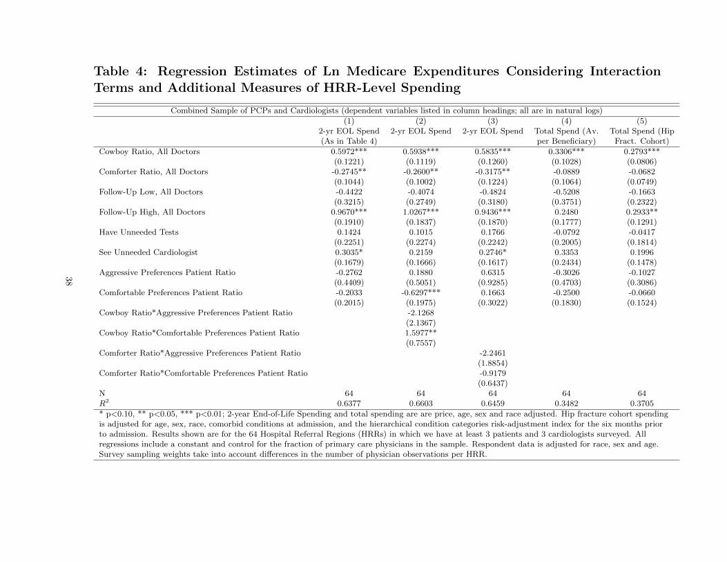
Table 4: Regression Estimates of Ln Medicare Expenditures Considering InteractionTerms and Additional Measures of HRR-Level Spending

Combined Sample of PCPs and Cardiologists (dependent variables listed in column headings; all are in natural logs)

(1) (2) (3) (4) (5)2-yr EOL Spend 2-yr EOL Spend 2-yr EOL Spend Total Spend (Av. Total Spend (Hip(As in Table 4) per Beneficiary) Fract. Cohort)

Cowboy Ratio, All Doctors 0.5972*** 0.5938*** 0.5835*** 0.3306*** 0.2793***(0.1221) (0.1119) (0.1260) (0.1028) (0.0806)

Comforter Ratio, All Doctors -0.2745** -0.2600** -0.3175** -0.0889 -0.0682(0.1044) (0.1002) (0.1224) (0.1064) (0.0749)

Follow-Up Low, All Doctors -0.4422 -0.4074 -0.4824 -0.5208 -0.1663(0.3215) (0.2749) (0.3180) (0.3751) (0.2322)

Follow-Up High, All Doctors 0.9670*** 1.0267*** 0.9436*** 0.2480 0.2933**(0.1910) (0.1837) (0.1870) (0.1777) (0.1291)

Have Unneeded Tests 0.1424 0.1015 0.1766 -0.0792 -0.0417(0.2251) (0.2274) (0.2242) (0.2005) (0.1814)

See Unneeded Cardiologist 0.3035* 0.2159 0.2746* 0.3353 0.1996(0.1679) (0.1666) (0.1617) (0.2434) (0.1478)

Aggressive Preferences Patient Ratio -0.2762 0.1880 0.6315 -0.3026 -0.1027(0.4409) (0.5051) (0.9285) (0.4703) (0.3086)

Comfortable Preferences Patient Ratio -0.2033 -0.6297*** 0.1663 -0.2500 -0.0660(0.2015) (0.1975) (0.3022) (0.1830) (0.1524)

Cowboy Ratio*Aggressive Preferences Patient Ratio -2.1268(2.1367)

Cowboy Ratio*Comfortable Preferences Patient Ratio 1.5977**(0.7557)

Comforter Ratio*Aggressive Preferences Patient Ratio -2.2461(1.8854)

Comforter Ratio*Comfortable Preferences Patient Ratio -0.9179(0.6437)

N 64 64 64 64 64R2 0.6377 0.6603 0.6459 0.3482 0.3705

* p<0.10, ** p<0.05, *** p<0.01; 2-year End-of-Life Spending and total spending are are price, age, sex and race adjusted. Hip fracture cohort spendingis adjusted for age, sex, race, comorbid conditions at admission, and the hierarchical condition categories risk-adjustment index for the six months priorto admission. Results shown are for the 64 Hospital Referral Regions (HRRs) in which we have at least 3 patients and 3 cardiologists surveyed. Allregressions include a constant and control for the fraction of primary care physicians in the sample. Respondent data is adjusted for race, sex and age.Survey sampling weights take into account differences in the number of physician observations per HRR.

38

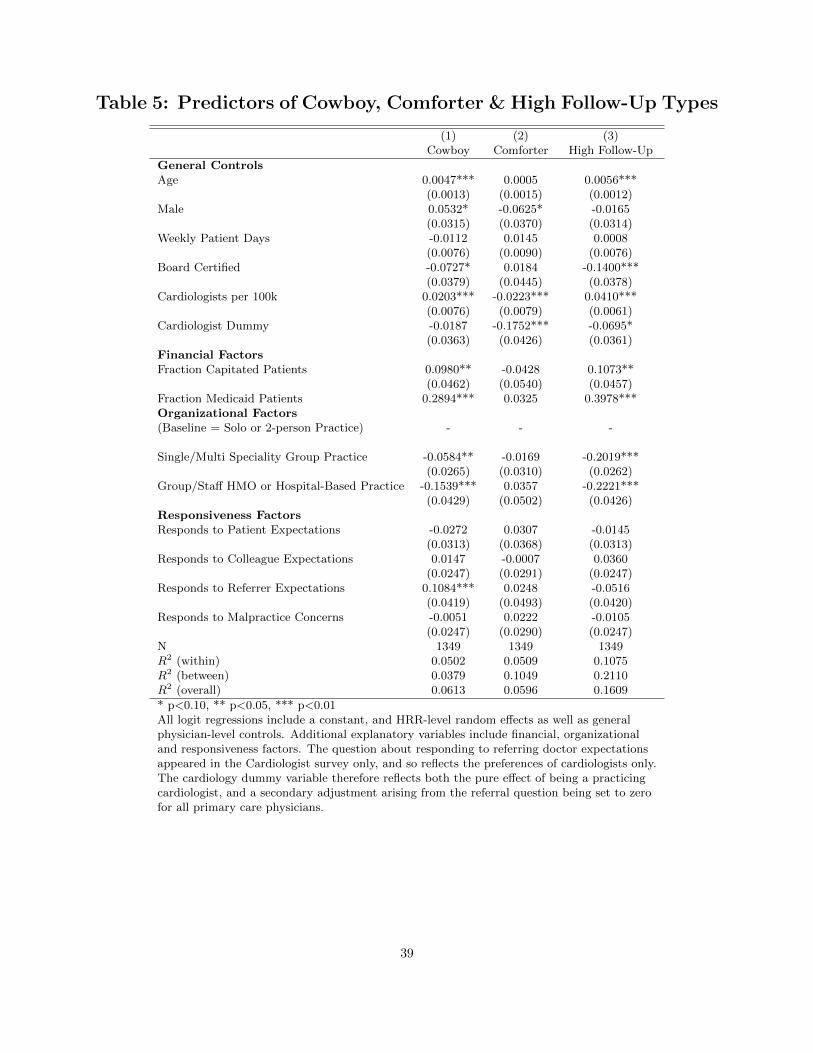
Table 5: Predictors of Cowboy, Comforter & High Follow-Up Types

(1) (2) (3)Cowboy Comforter High Follow-Up

General ControlsAge 0.0047*** 0.0005 0.0056***

(0.0013) (0.0015) (0.0012)Male 0.0532* -0.0625* -0.0165

(0.0315) (0.0370) (0.0314)Weekly Patient Days -0.0112 0.0145 0.0008

(0.0076) (0.0090) (0.0076)Board Certified -0.0727* 0.0184 -0.1400***

(0.0379) (0.0445) (0.0378)Cardiologists per 100k 0.0203*** -0.0223*** 0.0410***

(0.0076) (0.0079) (0.0061)Cardiologist Dummy -0.0187 -0.1752*** -0.0695*

(0.0363) (0.0426) (0.0361)Financial FactorsFraction Capitated Patients 0.0980** -0.0428 0.1073**

(0.0462) (0.0540) (0.0457)Fraction Medicaid Patients 0.2894*** 0.0325 0.3978***Organizational Factors(Baseline = Solo or 2-person Practice) - - -

Single/Multi Speciality Group Practice -0.0584** -0.0169 -0.2019***(0.0265) (0.0310) (0.0262)

Group/Staff HMO or Hospital-Based Practice -0.1539*** 0.0357 -0.2221***(0.0429) (0.0502) (0.0426)

Responsiveness FactorsResponds to Patient Expectations -0.0272 0.0307 -0.0145

(0.0313) (0.0368) (0.0313)Responds to Colleague Expectations 0.0147 -0.0007 0.0360

(0.0247) (0.0291) (0.0247)Responds to Referrer Expectations 0.1084*** 0.0248 -0.0516

(0.0419) (0.0493) (0.0420)Responds to Malpractice Concerns -0.0051 0.0222 -0.0105

(0.0247) (0.0290) (0.0247)N 1349 1349 1349R2 (within) 0.0502 0.0509 0.1075R2 (between) 0.0379 0.1049 0.2110R2 (overall) 0.0613 0.0596 0.1609

* p<0.10, ** p<0.05, *** p<0.01All logit regressions include a constant, and HRR-level random effects as well as generalphysician-level controls. Additional explanatory variables include financial, organizationaland responsiveness factors. The question about responding to referring doctor expectationsappeared in the Cardiologist survey only, and so reflects the preferences of cardiologists only.The cardiology dummy variable therefore reflects both the pure effect of being a practicingcardiologist, and a secondary adjustment arising from the referral question being set to zerofor all primary care physicians.

39

Appendix A: Clinical Vignettes and Response Options for Patients,Cardiologists and Primary Care Physicians

Panel I: Patient Questions

SCENARIO 1- Questions relating to less-severe cardiac care preferences: Suppose you noticed a mild but definitechest pain when walking up stairs....Suppose you went to your regular doctor for that chest pain and your doctor didnot think you needed any special tests but you could have some tests if you wanted.a) If the tests did not have any health risks, do you think you would probably have the tests or probably not havethem?

a - have testsb - not have tests

b) Suppose your doctor told you he or she did not think you needed to see a heart specialist, but you could see one ifyou wanted. Do you think you would probably ask to see a specialist, or probably not see a specialist?

a - see specialistb - not see specialist

SCENARIO 2 - Questions relating to end of life care preferences: The next set of questions are about care a patientmay receive during the last months of life. Remember, you can skip any question you don’t want to answer. Supposethat you had a very serious illness. Imagine that no one knew exactly how long you would live, but your doctors saidyou almost certainly would live less than 1 year.a) If you reached the point at which you were feeling bad all the time, would you want drugs that would make you feelbetter, even if they might shorten your life?

a - yes: drugsb - no

b1) If you needed a respirator to stay alive, and it would extend your life for a week, would you want to be put on arespirator?b2) If it would extend your life for a month, would you want to be put on a respirator?

a - yes: respiratorb - no

Answers other than “yes” or “no” (e.g., “not concerned” or “I dont know”) are treated as missing data. Itemnon-response was less than 1% among eligible respondents.

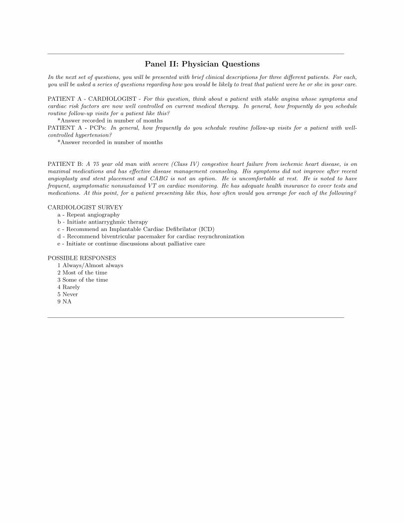
Panel II: Physician Questions

In the next set of questions, you will be presented with brief clinical descriptions for three different patients. For each,you will be asked a series of questions regarding how you would be likely to treat that patient were he or she in your care.

PATIENT A - CARDIOLOGIST - For this question, think about a patient with stable angina whose symptoms andcardiac risk factors are now well controlled on current medical therapy. In general, how frequently do you scheduleroutine follow-up visits for a patient like this?

*Answer recorded in number of monthsPATIENT A - PCPs: In general, how frequently do you schedule routine follow-up visits for a patient with well-controlled hypertension?

*Answer recorded in number of months

PATIENT B: A 75 year old man with severe (Class IV) congestive heart failure from ischemic heart disease, is onmaximal medications and has effective disease management counseling. His symptoms did not improve after recentangioplasty and stent placement and CABG is not an option. He is uncomfortable at rest. He is noted to havefrequent, asymptomatic nonsustained VT on cardiac monitoring. He has adequate health insurance to cover tests andmedications. At this point, for a patient presenting like this, how often would you arrange for each of the following?

CARDIOLOGIST SURVEYa - Repeat angiographyb - Initiate antiarryghmic therapyc - Recommend an Implantable Cardiac Defibrilator (ICD)d - Recommend biventricular pacemaker for cardiac resynchronizatione - Initiate or continue discussions about palliative care

POSSIBLE RESPONSES1 Always/Almost always2 Most of the time3 Some of the time4 Rarely5 Never9 NA

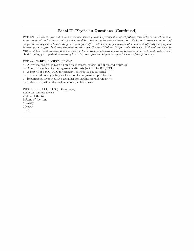
Panel II: Physician Questions (Continued)

PATIENT C: An 85 year old male patient has severe (Class IV) congestive heart failure from ischemic heart disease,is on maximal medications, and is not a candidate for coronary revascularization. He is on 2 liters per minute ofsupplemental oxygen at home. He presents to your office with worsening shortness of breath and difficulty sleeping dueto orthopnea. Office chest xray confirms severe congestive heart failure. Oxygen saturation was 85% and increased to94% on 4 liters and the patient is more comfortable. He has adequate health insurance to cover tests and medications.At this point, for a patient presenting like this, how often would you arrange for each of the following?

PCP and CARDIOLOGIST SURVEYa - Allow the patient to return home on increased oxygen and increased diureticsb - Admit to the hospital for aggressive diuresis (not to the ICU/CCU)c - Admit to the ICU/CCU for intensive therapy and monitoringd - Place a pulmonary artery catheter for hemodynamic optimizatione - Recommend biventricular pacemaker for cardiac resynchronizationf - Initiate or continue discussions about palliative care

POSSIBLE RESPONSES (both surveys)1 Always/Almost always2 Most of the time3 Some of the time4 Rarely5 Never9 NA

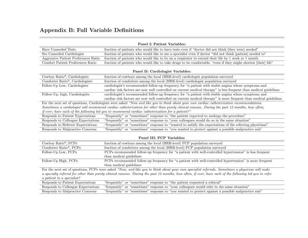
Appendix B: Full Variable Definitions

Panel I: Patient Variables:

Have Unneeded Tests fraction of patients who would like to have tests even if “doctor did not think [they were] needed”

See Unneeded Cardiologist fraction of patients who would like to see a specialist even if doctor “did not think [patient] needed to”

Aggressive Patient Preferences Ratio fraction of patients who would like to be on a respirator to extend their life by 1 week or 1 month

Comfort Patient Preferences Ratio fraction of patients who would like to take drugs to be comfortable, “even if they might shorten [their] life”

Panel II: Cardiologist Variables:

Cowboy Ratio*, Cardiologists fraction of cowboys among the local (HRR-level) cardiologist population surveyed

Comforter Ratio*, Cardiologists fraction of comforters among the local (HRR-level) cardiologist population surveyed

Follow-Up Low, Cardiologists cardiologist’s recommended follow-up frequency for “a patient with stable angina whose symptoms andcardiac risk factors are now well controlled on current medical therapy” is less frequent than medical guidelines

Follow-Up, high, Cardiologists cardiologist’s recommended follow-up frequency for “a patient with stable angina whose symptoms andcardiac risk factors are now well controlled on current medical therapy” is more frequent than medical guidelines

For the next set of questions, Cardiologists were asked “Now wed like you to think about your own cardiac catheterization recommendations.Sometimes a cardiologist will recommend cardiac catheterization for other than purely clinical reasons. During the past 12 months, how often,if ever, have each of the following led you to recommend cardiac catheterization for a patient?”

Responds to Patient Expectations “frequently” or “sometimes” response to “the patient expected to undergo the procedure”

Responds to Colleague Expectations “frequently” or “sometimes” response to “your colleagues would do so in the same situation”

Responds to Referrer Expectations “frequently” or “sometimes” response to “wanted to satisfy the expectations of the referring physicians”

Responds to Malpractice Concerns “frequently” or “sometimes” response to “you wanted to protect against a possible malpractice suit’

Panel III: PCP Variables:

Cowboy Ratio*, PCPs fraction of cowboys among the local (HRR-level) PCP population surveyed

Comforter Ratio*, PCPs fraction of comforters among the local (HRR-level) PCP population surveyed

Follow-Up Low, PCPs PCPs recommended follow-up frequency for “a patient with well-controlled hypertension” is less frequentthan medical guidelines

Follow-Up High, PCPs PCPs recommended follow-up frequency for “a patient with well-controlled hypertension” is more frequentthan medical guidelines

For the next set of questions, PCPs were asked “Now, wed like you to think about your own specialist referrals. Sometimes a physician will makea specialty referral for other than purely clinical reasons. During the past 12 months, how often, if ever, have each of the following led you to refera patient to a specialist?

Responds to Patient Expectations “frequently” or “sometimes” response to “the patient requested a referral”

Responds to Colleague Expectations “frequently” or “sometimes” response to “your colleagues would refer in the same situation”

Responds to Malpractice Concerns “frequently” or “sometimes” response to “you wanted to protect against a possible malpractice suit”

Panel IV: Other Variables (all physicians):

Practice Type 1 physician is part of a solo or 2-person practicePractice Type 2 physician is part of a singe or multi speciality group practicePractice Type 3 physician is part of a group or staff model HMO or a Hospital based practice

Fraction Capitated Patients fraction of patients for which physician is reimbursed on a captiated basis

Fraction Medicaid Patients fraction of patients a physician sees who are on Medicaid

Weekly Patients Days number of days per week a physician spends seeing patients

Age physician’s age in years

Board Certified physician is currently board certified in her speciality

Cardiologists per 100k cardiologists per 100,000 Medicare beneficiaries in HRR of practice as reported in the 2005 Dartmouth Atlas

Notes: detailed explanations of the algorithm used to define “Cowboys” (physicians aggressive beyond clinical guidelines) and “Comforters”(physicians who show a strong likelihood of recommending palliative and comfort-oriented care) are described in the paper. The indicator for“Aggressive Patient Preferences” combines two questions: affirmative responses to both part b1 and b2 of Patient Scenario 2 (see AppendixA above for original survey text)

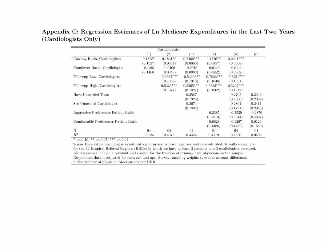
Appendix C: Regression Estimates of Ln Medicare Expenditures in the Last Two Years(Cardiologists Only)

Cardiologists

(1) (2) (3) (4) (5) (6)

Cowboy Ratio, Cardiologists 0.1825* 0.1831** 0.2460*** 0.1726** 0.2391***(0.1027) (0.0864) (0.0883) (0.0857) (0.0868)

Comforter Ratio, Cardiologists -0.1261 -0.0400 -0.0016 -0.0449 -0.0111(0.1100) (0.0848) (0.0903) (0.0852) (0.0862)

Followup Low, Cardiologists -0.6662*** -0.5460*** -0.7836*** -0.6951***(0.1062) (0.1373) (0.1648) (0.1691)

Followup High, Cardiologists 0.5323*** 0.5265*** 0.5333*** 0.5292***(0.1077) (0.1027) (0.1062) (0.1017)

Have Unneeded Tests 0.2587 0.2705 0.2343(0.1925) (0.2066) (0.2302)

See Unneeded Cardiologist 0.2674 0.2894 0.2411(0.1834) (0.1791) (0.2083)

Aggressive Preferences Patient Ratio -0.2385 -0.2539 -0.2870(0.3013) (0.3044) (0.4397)

Comfortable Preferences Patient Ratio -0.0628 -0.1267 0.0120(0.1488) (0.1482) (0.1559)

N 64 64 64 64 64 64R2 0.0535 0.4073 0.4446 0.4119 0.4530 0.0406

* p<0.10, ** p<0.05, *** p<0.012-year End-of-Life Spending is in natural log form and is price, age, sex and race adjusted. Results shown arefor the 64 Hospital Referral Regions (HRRs) in which we have at least 3 patients and 3 cardiologists surveyed.All regressions include a constant and control for the fraction of primary care physicians in the sample.Respondent data is adjusted for race, sex and age. Survey sampling weights take into account differencesin the number of physician observations per HRR.

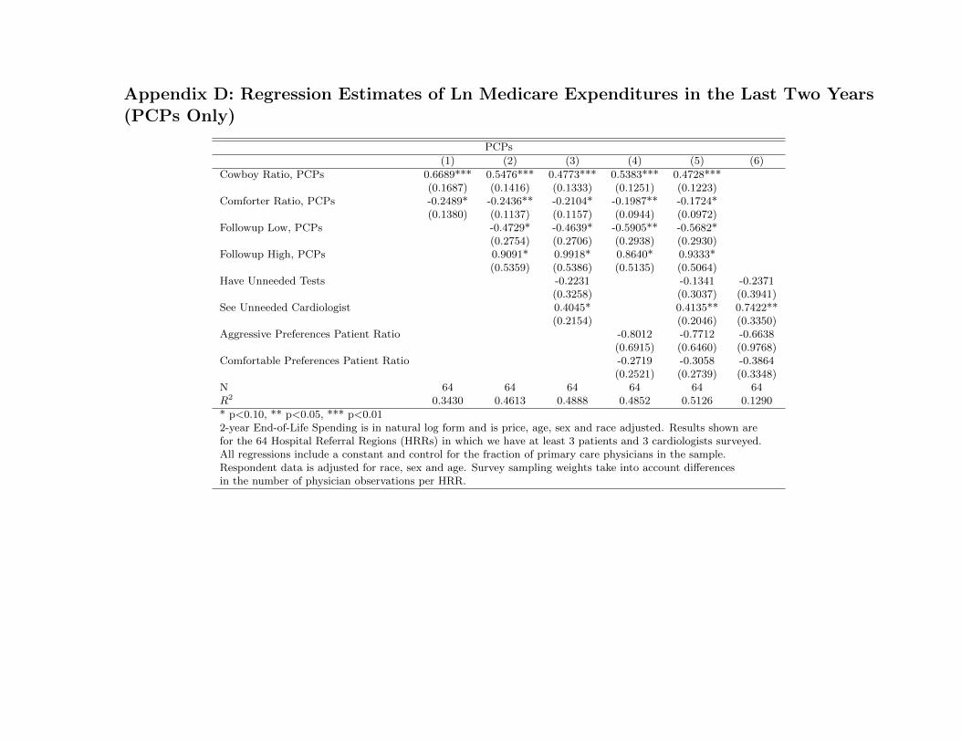
Appendix D: Regression Estimates of Ln Medicare Expenditures in the Last Two Years(PCPs Only)

PCPs

(1) (2) (3) (4) (5) (6)

Cowboy Ratio, PCPs 0.6689*** 0.5476*** 0.4773*** 0.5383*** 0.4728***(0.1687) (0.1416) (0.1333) (0.1251) (0.1223)

Comforter Ratio, PCPs -0.2489* -0.2436** -0.2104* -0.1987** -0.1724*(0.1380) (0.1137) (0.1157) (0.0944) (0.0972)

Followup Low, PCPs -0.4729* -0.4639* -0.5905** -0.5682*(0.2754) (0.2706) (0.2938) (0.2930)

Followup High, PCPs 0.9091* 0.9918* 0.8640* 0.9333*(0.5359) (0.5386) (0.5135) (0.5064)

Have Unneeded Tests -0.2231 -0.1341 -0.2371(0.3258) (0.3037) (0.3941)

See Unneeded Cardiologist 0.4045* 0.4135** 0.7422**(0.2154) (0.2046) (0.3350)

Aggressive Preferences Patient Ratio -0.8012 -0.7712 -0.6638(0.6915) (0.6460) (0.9768)

Comfortable Preferences Patient Ratio -0.2719 -0.3058 -0.3864(0.2521) (0.2739) (0.3348)

N 64 64 64 64 64 64R2 0.3430 0.4613 0.4888 0.4852 0.5126 0.1290

* p<0.10, ** p<0.05, *** p<0.012-year End-of-Life Spending is in natural log form and is price, age, sex and race adjusted. Results shown arefor the 64 Hospital Referral Regions (HRRs) in which we have at least 3 patients and 3 cardiologists surveyed.All regressions include a constant and control for the fraction of primary care physicians in the sample.Respondent data is adjusted for race, sex and age. Survey sampling weights take into account differencesin the number of physician observations per HRR.

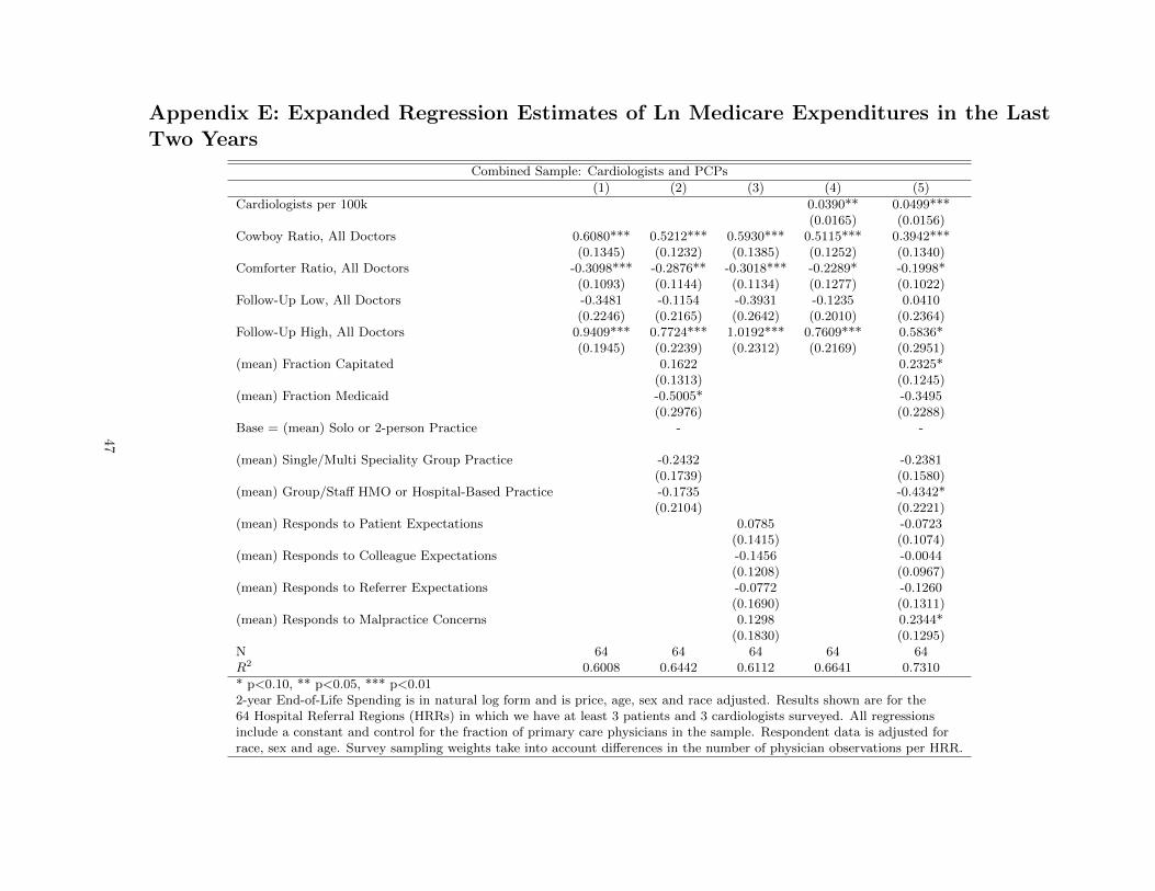
Appendix E: Expanded Regression Estimates of Ln Medicare Expenditures in the LastTwo Years

Combined Sample: Cardiologists and PCPs

(1) (2) (3) (4) (5)

Cardiologists per 100k 0.0390** 0.0499***(0.0165) (0.0156)

Cowboy Ratio, All Doctors 0.6080*** 0.5212*** 0.5930*** 0.5115*** 0.3942***(0.1345) (0.1232) (0.1385) (0.1252) (0.1340)

Comforter Ratio, All Doctors -0.3098*** -0.2876** -0.3018*** -0.2289* -0.1998*(0.1093) (0.1144) (0.1134) (0.1277) (0.1022)

Follow-Up Low, All Doctors -0.3481 -0.1154 -0.3931 -0.1235 0.0410(0.2246) (0.2165) (0.2642) (0.2010) (0.2364)

Follow-Up High, All Doctors 0.9409*** 0.7724*** 1.0192*** 0.7609*** 0.5836*(0.1945) (0.2239) (0.2312) (0.2169) (0.2951)

(mean) Fraction Capitated 0.1622 0.2325*(0.1313) (0.1245)

(mean) Fraction Medicaid -0.5005* -0.3495(0.2976) (0.2288)

Base = (mean) Solo or 2-person Practice - -

(mean) Single/Multi Speciality Group Practice -0.2432 -0.2381(0.1739) (0.1580)

(mean) Group/Staff HMO or Hospital-Based Practice -0.1735 -0.4342*(0.2104) (0.2221)

(mean) Responds to Patient Expectations 0.0785 -0.0723(0.1415) (0.1074)

(mean) Responds to Colleague Expectations -0.1456 -0.0044(0.1208) (0.0967)

(mean) Responds to Referrer Expectations -0.0772 -0.1260(0.1690) (0.1311)

(mean) Responds to Malpractice Concerns 0.1298 0.2344*(0.1830) (0.1295)

N 64 64 64 64 64R2 0.6008 0.6442 0.6112 0.6641 0.7310

* p<0.10, ** p<0.05, *** p<0.012-year End-of-Life Spending is in natural log form and is price, age, sex and race adjusted. Results shown are for the64 Hospital Referral Regions (HRRs) in which we have at least 3 patients and 3 cardiologists surveyed. All regressionsinclude a constant and control for the fraction of primary care physicians in the sample. Respondent data is adjusted forrace, sex and age. Survey sampling weights take into account differences in the number of physician observations per HRR.

47

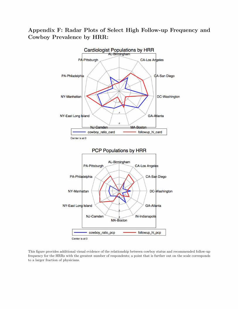
Appendix F: Radar Plots of Select High Follow-up Frequency andCowboy Prevalence by HRR:

This figure provides additional visual evidence of the relationship between cowboy status and recommended follow-upfrequency for the HRRs with the greatest number of respondents; a point that is further out on the scale correspondsto a larger fraction of physicians.