physician beliefs and patient preferences: a new look at ... · pdf filewe test the model...
TRANSCRIPT
0
26 November 2012
Physician Beliefs and Patient Preferences: A New Look at Supplier-Induced Demand
David Cutler
Harvard University National Bureau of Economic Research
Jonathan Skinner Department of Economics, Dartmouth College
Dartmouth Institute for Health Policy and Clinical Practice National Bureau of Economic Research
Ariel Dora Stern Harvard University
David Wennberg Dartmouth Institute for Health Policy and Clinical Practice
Version 1.0: Please do not quote
Abstract Supplier-induced demand is the idea that physicians face trade-offs between patient benefits and their own income, and that equilibrium behavior partly reflects financial benefit. We embed supplier-induced demand in a model where there is variation in patient preferences and where physician behavior is affected by both organizational factors and professional beliefs. We test the model using three surveys. The first asked elderly Medicare enrollees about preferences for end-of-life care. The second and third asked cardiologists and primary care physicians, respectively, about organizational and financial pressures, and give them vignettes on how they would treat specific patients. The surveys were linked to Medicare end-of-life utilization data at the hospital-referral region (HRR) geographical level. Our results do not support a large role for patient demand or direct physician financial considerations in explaining regional differences in utilization. While organizational factors influence physician behavior, the best explanation for large observed variations in treatment patterns is physician beliefs about their own productivity. Many physician beliefs are more aggressive than professional guidelines, suggesting the presence of considerable waste in U.S. health care. Comments by Amitabh Chandra, Nancy Morden, Allison Rosen, Gregg Roth, Tisamarie Sherry, Sara Nadel, and seminar participants at Harvard University and Dartmouth were exceedingly helpful. We are particularly grateful to F. Jack Fowler and Patricia Gallagher of the University of Massachusetts Boston for helping to develop the patient and physician questionnaires. Funding from the National Institute on Aging (T32-AG000186-23 to the National Bureau of Economic Research and P01-AG019783 to Dartmouth) and LEAP at Harvard University (to Skinner) is gratefully acknowledged. Survey data are available at www.intensity.dartmouth.edu.

1
I. Introduction
Regional variations in rates of medical treatments are widespread in the United States and
other countries. For example, in the U.S. Medicare population over age 65, rates of back surgery
range from 2.0 per 1,000 in Manhattan, NY, to 9.3 in Eugene, OR (Dartmouth Atlas, 2012), while
in England rates of tonsillectomies vary across regions seven-fold (Suleman et al., 2010). Price-
adjusted expenditures range from $6,424 in Salem, OR to $15,571 in Miami, FL, with most of the
variation unexplained by regional differences in patient illness or poverty (Sutherland, et al.,
2010; Zuckerman et al., 2010).
Then what drives such variation? One obvious possibility is patient demand: access,
income and price differences across regions. In the U.S. Medicare program, however, everyone
has a similar primary insurance policy,1 and costs paid by individuals are relatively low, while the
income-elasticity of demand for healthcare utilization appears to be modest at best (McClellan
and Skinner, 2006). Yet heterogeneity in patient preferences for care may still play a role. In the
case of mild coronary disease, some patients may prefer surgery to insert stents, while others may
prefer diet, exercise, and medication as first line treatments. If patients with similar preferences
group together geographically – for example, people who value intensive treatments live in areas
with ‘world-class’ interventional physicians – patient preference heterogeneity could lead to
regional variation in equilibrium outcomes (Mandelblatt et al., 2012; Anthony et al., 2010).
Another source of variations arises from the supply side, with the most obvious
explanation differences across regions in price margins. In a fully specified principle-agent model
(McGuire and Pauly, 1991), if prices are high enough (and income scarce), the patient’s
1 Access to physicians is universal in the traditional Medicare program. The presence of supplemental insurance coverage differs across the country, but most studies do not find that these difference affect utilization by more than a small degree.

2
physician-agent recommends care beyond what is medically appropriate, leading to the canonical
“supplier-induced demand.” While physician utilization has been shown to be sensitive to prices
(Jacobson et al., 2006, Clemens and Gottlieb, 2011), it would be difficult to explain observed
Medicare variations using price margins alone, since reimbursement rates are set administratively
and patients pay little for care out-of-pocket.
Variation in desired supply may also result from non-monetary factors. Physicians may
respond to organizational pressure or peer pressure to perform more procedures (de Jong, 2008),
even if their current income is no higher as a consequence. More generally, physicians may have
different beliefs about appropriate treatments, particularly for treatments where there are few
professional guidelines (Wennberg and Gittelsohn, 1975). These in turn may arise because of
differences in where they were trained (Epstein and Nicholson, 2009), or their personal
experience with different treatments (Levine-Taub et al., 2011). If this variation is correlated
spatially – for example, intensive physicians are more likely to hire other physicians with similar
views – the resulting regional differences in perception about optimal treatment could explain
regional variations in equilibrium spending outcomes.
While we have good estimates of how changes in prices and income affect physician and
patient behavior (e.g., Gruber and Owings, 1996; Jacobson et al., 2006; Colla et al., 2012;
Chandra et al., 2010), it is far more difficult to estimate an equilibrium model that disentangles
physician preferences from patient preferences and other factors at a point in time. A good
illustration of the risks of seeking to estimate parameters of such models was best illustrated by
Dranove (1994), who showed that the use of then-standard identification strategies implied the
nonsensical result that obstetricians “caused” births. For this reason, we use a new approach to
identification: “strategic” surveys (as in Ameriks et al., 2010) that ask providers and patients

3
about motivations, clinical beliefs, and preferences, and are in turn linked to equilibrium measures
of utilization at the regional level.
We use this survey-based approach to first examine whether patient or physician
preferences are more important in explaining regional variations in care. Patient preferences are
measured by a survey of 2,515 Medicare enrollees age 65 and older asking about their preferences
for a variety of aggressive care interventions.2 We focus on questions most germane to patients
with severe conditions, where there are often clear tradeoffs between painful and invasive
procedures with modest potential benefit, versus palliative care where the emphasis is on comfort
rather than extra weeks of life.
Physician beliefs and opinions are captured by two surveys, one of cardiologists (N = 516)
and the second of primary care doctors (N=807). Both cardiologists and primary care doctors
(general internists and family practitioners) were presented with vignettes for four (largely
overlapping) elderly individuals with chronic health conditions, and asked how they would treat
each one. These hypothetical patients ranged the gamut of severity from stable angina (less
severe) to late-stage Class IV congestive heart failure (very severe). Based on their responses, we
characterized physicians along two separate dimensions: those who recommended intensive care
beyond that suggested by the medical literature (or “cowboys”), and those who were more likely
to recommend palliative care for the very severely ill patients (“comforters”).
We use these surveys to measure the relative importance of demand and supply factors in
determining equilibrium outcomes. Specifically, we relate area-level Medicare spending and
utilization of particular procedures to area average preferences of patients for receiving additional
2 The survey, funded by the National Institute on Aging, was conducted in 2005 by The Center for Survey Research (CSR) at the University of Massachusetts, Boston and Dartmouth (Geisel) Medical School under the direction of F. Jack Fowler and Patricia Gallagher.

4
care and local preferences of physicians for providing additional care. Our results are very clear –
even with very small numbers (6-10 physicians per area), the impact of physician preferences is
large. In contrast, patient preferences explain less of the variation.
We then try to understand why physicians have the preferences they do by relating
physicians’ views about optimal treatment to a wide variety of questions about the nature of the
respondent’s practice (how many Medicaid patients, how many capitated patients), organizational
pressures (the frequency with which the cardiologist accommodated referring physicians
expectations, provided treatments for patients who expected but didn’t need them) and financial
pressures that may affect their clinical decisions.
We find that only a small fraction of physicians claim to have made recent intervention
decisions as a result of financial considerations alone. On the other hand, we find that
organizational factors reflected by “pressure to accommodate” either patients (providing
treatments that are not needed) or referring physicians (doing procedures to keep them happy)
were much more common among responding cardiologists, exerting a small but significant impact
on physician decisions. Ultimately, the largest degree of regional variation in utilization appears
to be explained by physician beliefs. These results are strongly suggestive therefore of
considerable waste in U.S. healthcare: high levels of expenditures for treatments with no evidence
of medical value that patients prefer not to have.
II. A Model of Variation in Utilization
We develop a simple model of patient demand and physician supply and test the
implications of the model using individual-level data from both patients and physicians, linked by
geography and patterns of service utilization. The demand side of the model is a standard one; the
indirect utility function is a function of out-of-pocket prices (which are generally low), income,

5
and preferences for care; V = V(p, Y, η), where p denotes out-of-pocket price, Y income, and η a
measure of preferences for intensive care. Solving this for optimal intensity of care, x, yields xD.
We assume that xD is the patient’s demand for the quantity of procedures when they are first
stepping into the physician’s office, prior to any demand “inducement.” We can approximate xD
(that is, the cumulative impact of these factors on the demand for health care intensity) by the use
of our patient survey with hypothetical questions about preferences for more aggressive care near
the end of life.
We focus in detail on the model of physician behavior. Our primary assumption is that
physicians seek to maximize the perceived health of their patient, s(x), by appropriate choice of
inputs x, subject to patient demand (xD), financial considerations, and organizational factors.
Note that s(x) includes both survival and quality of life, for example quality-adjusted life years
(QALYs). The quantity of input x can refer either to the intensity with which a given patient is
treated, or the number of patients treated with a given procedure (or some combination of both).
Individual physicians are assumed to be price-takers (once their networks have negotiated
prices with insurance companies), but may face a wide range of reimbursement rates from private
insurance, Medicare, and Medicaid. The model is therefore simpler than models in which
hospital groups and physicians jointly determine quantity, quality, and price (Pauly, 1980) or
where physicians exercise market power over patients to provide them with “too much” health
care (McGuire, 2011). Following Chandra and Skinner (2012), the Lagrangian for a given health
care provider can be written:
(1) ℒ = Ψ𝑠(𝑥) + Ω(𝑊 + 𝜋𝑥 − 𝑅) −𝜙(|𝑥 − 𝑥𝐷|)− 𝜑(|𝑥 − 𝑥𝑂|)
where Ψ is the social value of improving the quality or quantity of life (and thus reflects the value
to the physician of helping her patient), Ω is the utility function of the physician’s own income,

6
comprising her fixed payment W (in a salaried setting, for example) as well as the incremental
“profits” from the incremental procedure, π. 3 Note that π may be negative or positive depending
on the type of procedure and who is paying for it. Finally, R is fixed costs; higher R results in a
higher marginal utility of income and hence greater attention paid to financial constraints
(McGuire, 2011).
The third term represents the loss in provider utility arising from the deviation between
what the provider prescribes (x) and what the patient wants (xD). This function could reflect
classic supplier-induced demand – from the physician’s point of view, xD is too low relative to the
physician’s belief in optimal x, and thus more care is provided than the patient thinks optimal.
But the function also reflects the extent to which physicians are acting as the agent of the possibly
misinformed patient – for example when the patient wants a procedure that the physician does not
feel is medically appropriate.
The fourth term reflects a parallel influence on physician decision making by
organizational factors that do not directly affect financial rewards, such as (physician) peer
pressure or concerns about keeping in referring physicians’ good graces. For example, Moliter
(2011) showed that when cardiologists move to a new region, their practice style adjusts partially
to those of their new peers. As many cardiologists face an “eat what you kill” environment in
which their business comes from referral networks, they have strong incentives to keep their
referring primary care physicians happy.4
The first-order condition for (1) is:
3 We ignore here capacity constraints, such as the supply of hospital or ICU beds, or the availability of MRIs and catheterization laboratories; see for example Wennberg, et al. (2002) and especially Wennberg (2010). These are likely to be more important in non-U.S. health care systems with a greater degree of centralized planning for specialized facilities. 4 This last example emphasizes the somewhat arbitrary distinction between organizational pressures (not challenging the clinical judgment of fellow physicians) and financial pressures.

7
(2) Ψ𝑠′(𝑥) = −Ω′𝜋 + 𝜙′ + 𝜑′ ≡ 𝜆
That is, physicians provide care up to the point where the choice of x reflects a balance between
the perceived social marginal value of health or functioning, Ψs′(x), versus factors summarized by
λ: (a) the resulting incremental change in net income π, weighted by the importance of financial
resources Ω′π, (b) the incremental disutility (if any) from moving patient demand away from
where it was originally when the patient entered the doctor’s office, and (c) how much the
physician’s own choice of x deviates from the organization’s perceived optimal level of
intervention, xo, and the incremental responsiveness of the physician to such informal pressures,
𝜙′.
In the context of this model, there are two ways to define conventional “supplier-induced
demand.” One is simply the presence of any induced demand, if actual x > xD, so that the patient
receives more than originally anticipated at a given price and income (that is, the patient demand
curve shifts to the right). This is still quite benign; the patient after all seeks out the physician’s
opinion for a reason, so xD (prior to seeing the physician) may optimally change after the visit.
More relevant then is the sign of s′(x) when evaluated at xD; does the change in demand enhance
health outcomes? An alternative definition is that supplier-induced demand exists when the
incremental care does not help the patient, (McGuire, 2011) i.e. s′(z) ≤ 0 as z ranges from x to xD.
The average benefit may still be positive, even if at the margin treatment is too aggressive.
Consider Figure 1, showing both Ψs'(x) and λ, which for simplicity we assume to be
constant for all x. Note also the key assumption that patients are sorted in order from most
appropriate to least appropriate for treatment, thus describing a downward sloping Ψs'(x) curve
(Baicker, Buckles, and Chandra, 2006). Equilibrium is where Ψs'(x) = λ, or at intensity level A in
Figure 1. A different set of constraints, arising perhaps from different reimbursement rates for
8
procedures, different capacity, patient demand, and other factors discussed above, could yield a
different λ*, and hence a different utilization rate. Note that all of these factors that have the
potential to affect the intensity of treatments involve a movement along the marginal benefit
curve, Ψs′(x).
But suppose that s′(x) differs across physicians – a shift in the productivity curve rather
than a movement along the curve. In Figure 1, Point C corresponds to greater level of intensity
than Point A when the physician believes that she is more productive for any level of x, so that
g′(x) > s′(x) for all x.5 For example, heart attack patients experience better outcomes from cardiac
interventions in regions with higher rates of revascularization, consistent with a Roy model of
occupational sorting (Chandra and Staiger, 2007). Because patients in regions with high
intervention rates actually benefit differentially from these interventions, this scenario would not
correspond to the classic “supplier-induced demand” story because surgical patients are not being
“over treated” or harmed.6
Physicians may also be overly optimistic with respect to their own or the prescribed
treatment’s productivity, leading to perceived benefits that exceed actual benefits. Baumann et al.
(1991) have documented the phenomenon of “macro uncertainty, micro certainty” in which
physicians and nurses are very sure that their treatment benefited the specific patient (micro
certainty) even when there is no general consensus on which procedure is more clinically
effective (macro uncertainty). Furthermore, much of the evidence from psychology and the
medical literature points to overconfidence in one’s own ability, leading to a natural bias towards
5 This would also hold if either the patient or physician placed a greater relative weight on the social value of treatments, so that Ω differed across physicians or patients. 6 Instead, the patient who fails to get surgery in the high-surgery regions suffers, because the cardiologists provide inadequate medical treatment to these patients (Chandra and Staiger, 2007).

9
doing more.7 For example, if the physician’s perceived benefit is g′(x) but the actual benefit is
s′(x) in Figure 1, then at point C, the incremental treatment harms the patient – even though the
physician does not believe she is trading off patient benefit for personal economic gain. In
equilibrium, this may appear consistent with the classic supplier-induced demand hypothesis –
higher expenditures that are not associated with better outcomes – but the cause is quite different;
the physician believes she is providing the optimal level of care, and that not providing the
additional care would have harmed the patient.
Identification in the Empirical Model. In general, it is very difficult to distinguish among
these different explanations for treatment variation; even highly detailed clinical data makes it
difficult to second-guess the patient’s condition (the physician generally knows far more about
that patient than the researcher does) and the physician’s motivation for doing what she did. In
studying motives for household saving, Ameriks et al. (2011) implemented “strategic” surveys to
identify their otherwise difficult-to-identify models.8 We follow this approach by using a similar
approach to ask potential patients regarding hypothetical end-of-life choices (that is, xD before
their interaction with the physician), and physicians about how they would treat patients with
severe (or less severe) diseases, and what factors in fact affected their beliefs. We do this by
using vignettes of hypothetical patients that are identical across physicians, avoiding the problems
inherent in trying to risk-adjust actual clinical data. Vignettes in clinical settings have been shown
7 There are often clear psychological biases towards doing more as well even in the absence of effectiveness; if the patient gets better anyway, the physician gets the credit, but if the patient gets worse, the physician has done everything she could to save the patient’s life. 8 As they noted, it was nearly impossible to distinguish among saving motives based solely on how much households saved. They used the survey questions to ask about how respondents valued outcomes that could be affected by savings, for example the disutility of having to qualify for Medicaid if they failed to save enough for retirement.

10
to predict closely what physicians actually do in practice (Peabody et al., 2004; Mandelblatt et al.,
2012; Dresselhaus et al., 2004).
Empirical Specification. In considering the empirical evidence, we seek to distinguish
among the different factors that we posit can explain λ-based variation, and perceived
productivity differences (s′(x) versus g′(x) in Figure 1) in explaining physician choices. We do
this by taking a first-order Taylor-series approximation of (2) for region i. This in turn yields a
linear equation that depends on all the factors implicit in the model.9 We can further rearrange
this equation into two basic components, demand factors ZD and supply factors ZS, along with an
error term εi:
(4) 𝑥𝑖 = �̅� + 𝑍𝑖𝐷 + 𝑍𝑖𝑆 + 𝜀𝑖.
The pure demand-side component is simply
(5) 𝑍𝑖𝐷 = 1𝑀ϕ′(|𝑥𝑖𝐷 − 𝑥𝐷|)
or the impact of patient demand on actual utilization. By contrast, there are more factors involved
on the supply-side:
(6) 𝑍𝑖𝑆 = 1𝑀
{[Ω′Δπ + πΔΩ′] − Δ𝜙′(|𝑥 − 𝑥𝐷|) + [𝜑′Δ𝑥𝑂 + Δ𝜙′(|𝑥 − 𝑥𝑂|)] + [𝑠𝑖′(�̅�)−
�̅�′(�̅�)]}
The first term in brackets reflects how financial incentives affect utilization, whether because of
variations in profitability across providers (where Δπ denotes the deviation of net reimbursements
from its mean for provider i), or because physicians are more or less attuned to differences in
financial rewards (ΔΩ′). The second term on the RHS of (5) captures the willingness of the
physician to respond to differences in patient demand – that is, how willing are they to 9 The Taylor-series approximation is given by: 𝑥𝑖 = �̅� + 1
𝑀{[𝑠𝑖′(�̅�)− �̅�′(x�)] + [Ω′Δπ + πΔΩ′]−
[ϕ′Δx𝐷 + Δ𝜙′(𝑥 − 𝑥𝐷) + [𝜑′Δ𝑥𝑂 + Δ𝜙′(𝑥 − 𝑥𝑂)]}. Note that Δ here denotes deviation from the sample mean.
11
accommodate what patients want (even if the physician doesn’t agree with the patient’s
assessment). (This term reflects an interaction between demand and supply; for convenience we
include it under supply.) The third tem in brackets represents organizational effects, both
differences in organizational goals (which we do not measure), but also how willing the physician
is to accommodate those goals, reflected in a larger φ’. The fourth term measures the impact of
different physician beliefs about productivity of the treatment affect x. Note that these effects are
scaled by 1/M, where M = -s” + πΩ”, so that the magnitude of the effects will be larger the
smaller is the degree of diminishing returns to treatment -s” – that is, if there are many patients
who might (barely) benefit from the treatment, strongly-held opinions can lead to highly variable
treatment levels and intensities (Chandra and Skinner, 2012).
Estimation Strategy. We focus primarily on equations (4)-(6) above in our estimation
strategy. We define ZD to be a measure of patient demand for treatment, based on the survey
questionnaire of patients asking them about preferences towards end-of-life care. Note that for
most of those surveyed, ZD corresponds to xD because the questions reflect general preferences for
care prior to a specific interaction with a potentially demand-inducing physician or nurse. The
survey responses are also assumed to reflect the economic characteristics of the individual, such
as copayment prices and household income.
Similarly, we define ZS to be a composite measure of supply, or the physician’s preferred
treatment strategy based on her responses to the cardiologist survey questions. A higher value of
ZS is consistent with a more expensive treatment of unknown effectiveness. Thus if we think of
the two hypothetical congestive heart failure (CHF) patients in the survey as having very small
(and potentially negative) marginal benefits from expensive medical interventions according to
the American College of Cardiology/American Heart Association (ACC/AHA) guidelines, the

12
responses of the physicians anchor the intersection of λ and Ψs′(x) near the zero vertical axis in
Figure 1, and predict either a low x (a “comfort” physician emphasizing palliative or home care)
or a high x (an “intense” physician who would readmit the patient for additional surgical
procedures) depending on the physician’s response.
Our indices for the overall intensity of physician’s treatments, ZS, are derived from the
vignettes (as described below) and implicitly assume that the physician’s responses to the
vignettes are “all in” (as in Equation 6), reflecting physician beliefs, but also the variety of
financial, organizational, and capacity-related constraints she faces. Alternatively, one could
interpret the physician’s responses to the vignettes as a pure response of beliefs (for example, how
one might answer for qualifying boards), and hence not reflecting the day-to-day realities of
practice. However, including the organizational and financial variables in addition to the vignette
estimates did not appreciably increase the explanatory power of these equations.
The constructs ZD and ZS are assumed to be measured in the same units as x, which we
define here as actual (dollar) utilization. In an ideal world, we would have multiple patient survey
and utilization data for each physician. But because we cannot link patients directly to physicians,
to estimate Equation (4) we first match supply and demand at the HRR level, and define x –
utilization – to be log inpatient Medicare expenditures in the last six months of life, adjusted for
age, sex, race, and differences in Medicare reimbursement rates across regions. Thus our first
estimation exercise is a regression of Equation (4) at the HRR level and asks the simple question
of how factors related to demand and supply can explain actual expenditures. If, in fact,
physicians acted as perfect agents of patient demand (so that ϕ’ is very large in magnitude) then
we would expect to find that ZD would predict actual utilization x, leaving little incremental
influence for ZS. Alternatively, the two measures could be quite collinear when physician

13
responses to the vignettes mirror patient demand, leading to a high overall F-statistic but
insignificant individual t-statistics on the regression coefficients.
The second set of equations are estimated at the level of individual physicians using the
survey data, where we ask which of the multiple factors best explain how physicians respond to
vignettes. Assuming that the vignettes are in fact predictive of actual utilization, we then ask
which of the financial, organizational, or other factors are most closely related to the vignette
responses. If in fact we cannot explain either vignette responses (or actual utilization) by
reference to factors related to λ, then we assume that the observed variation is the consequence of
physician beliefs, or shifts in the perceived marginal treatment curve Ψs′(x) to Ψg′(x), and
conversely.
III. Data
We use three sources of survey data from patients, cardiologists, and primary care
physicians (PCP); a description of the questions is provided in Table 1. Each survey was
conducted by the Center for Survey Research (CSR), University of Massachusetts Boston. Each
survey was in turn aggregated and matched to Medicare claims data for hospital referral regions
(HRRs). We consider each in turn.
Patient Survey. The survey sampling frame was all Medicare beneficiaries in the 20%
denominator file who were age 65 or older on July 1, 2003 (see Barnato et al., 2009, for details).
A simple random sample of 4,000 was drawn from this sample, and beneficiaries were contacted
both by phone and mail; the response rate was 65%, with the final sample used in the analysis
(which was limited to respondents who provided all variables of interest) contains a total of 1165
people.10 We used responses to 6 survey questions, and, following Barnato et al (2009) treated
10 The survey was conducted in both English and Spanish, and was piloted with 15 seniors in intensive one-on-one interviews to test construct validity.

14
answers other than “yes” or “no” (e.g., “not concerned” or “I don’t know”) as missing data. For
example, one question related to wanting to see a cardiologist: “Suppose your doctor told you he
or she did not think you needed to see a heart specialist, but you could see one if you wanted. Do
you think you would probably ask to see a specialist, or probably not see a specialist? There is
wide variation across regions in this answer; Figure 2 shows the fraction responding that they did
want to see a specialist by HRR.
Other questions concerned receiving too little care in the last year of life or receiving too
much care, preference for life-prolonging drugs with side-effects, for palliative drugs with
potential for life-shortening, and for mechanical ventilation.11 Item non-response was less than
1% among eligible respondents for each outcome measure. Other covariates were also included
in the study such as age, sex, and race/ethnicity, which we used to adjust in creating our HRR-
level measures to match Medicare spending measures.12
Cardiologist Survey. A total of 999 cardiologists were randomly selected to receive the
survey. Of these, 614 physicians responded for a response rate of 61.5%. Of the 614 individuals
in the sample, 597 self-identify as cardiologists, while 81 were missing crucial pieces of
information for the subsequent regression analysis. We used a final sample of 516 cardiologists
who responded with complete information about their own backgrounds, practices, medical and
surgical activity over the past year, and likely clinical interventions on three vignette patients
11 Another example: “Suppose you went to your regular doctor for that chest pain and your doctor did not think you needed any special tests but you could have some tests if you wanted. If the tests did not have any health risks, do you think you would probably have the tests or probably not have them?” (Binary response: have = 1/ not have = 2.) 12 We created race and ethnicity controls as mutually exclusive groups of non-Hispanic white, black, Hispanic, or “other.” Also available in the survey were education, whether the beneficiary reported financial strain, and three health status measures. However, we were interested in an overall measure of demand, and did not want to condition for factors such as patient income.

15
(discussed below). In total, the 516 physicians in our cardiologist survey practice in 188 HRRs,
67 of which have 3 or more physicians represented.
Primary Care Physician (PCP) Survey. These data come from a parallel survey to
estimate the impact of physician opinion on regional variations (CSR, 2010). A total of 1333
primary care physicians were randomly selected to receive the survey. The original sample
included oversamples of physicians in four targeted cities, two in areas of low intensity
(Minneapolis, MN; Rochester, NY) and two in areas of high intensity (Manhattan, NY; and
Miami, FL). The cities were defined by the Census Bureau designated Metropolitan Statistical
Area (MSA) for each city. The primary care physicians were defined as having a primary
specialty of Family Practice (FP), Internal Medicine (IM), or Internal Medicine/Family Practice
(IFP). Of the 1333 physicians surveyed, 840 responded for a response rate of 63%.
Medicare Utilization Data. We merge the survey responses with Medicare utilization data
on inpatient end-of-life spending from the Dartmouth Atlas of Health Care by Hospital Referral
Region (HRR). These spending measures adjust for the type of chronic disease (e.g., dementia,
cancer, pulmonary disease) as well as multiple conditions, and are specific to the years 2003-07.
These end-of-life measures are commonly used to instrument for health care intensity, (e.g.,
Fisher et al., 2003a,b; Doyle, 2011; Silber et al., 2010; Romley et al., 2011) and are also highly
correlated with other medical expenditure measures such as one-year expenditures following a
heart attack (Skinner et al., 2010).
We further adjust the measures for differences across regions in Medicare reimbursement
rates for cost-of-living differences, graduate medical education payments, and the
16
disproportionate share hospitals (DSH) program payments.13 Finally, because HRR expenditure
is on the left-hand side of the equation, we are mostly concerned about sampling error on the
right-hand side. For this reason, we focus on the 64 larger HRRs with at least 3 cardiologists and
2 primary care physician surveys. Of the 2515 Medicare enrollees in the patient survey, 1165
enrollees live in one of those 64 HRRs, for an average of 18 respondents per HRR.
IV. Medical Evaluation of Clinical Vignettes from the Physician Surveys
We begin with our first and simplest vignette for patient A from the cardiologist survey.14
The question reads: “Think about a patient with stable angina whose symptoms and cardiac risk
factors are now well controlled on current medical therapy. In general, how frequently do you
schedule routine follow-up visits?” The response is unbounded, and expressed in months, which
in practice ranged from 1 month to 24 months. Figure 3 presents the HRR-level means for all
regions with sample sizes of 3 or greater, weighted by the number of observations. We adopt the
inverse of this measure, the average number of prescribed follow-up visits per year, as our first of
three indices summarizing ZS. 15
Diagnosis and management of coronary artery disease, the cause of angina, is the most
common clinical issue faced by cardiologists on a day-to-day basis. How do these responses
correspond to the ACC/AHA guidelines on managing chronic stable angina? Actually, there are
no data to support any recommendation. In the absence of data, the guidelines call for a
13 Because these adjustments have not been created explicitly for end-of-life payments, in practice we use the overall price index (based on total per-capita expenditures) to adjust for differences in reimbursement rates across regions. 14 We order these questions differently from their chronological appearance in the survey. 15 One might argue that physicians in regions with (say) very sick patients may “fill in” missing characteristics of the vignettes, for example that their representative patients are also ones with poor support systems at home. Biases from such “fill-ins” could go in either direction; procedures like bypass surgery require considerable rehabilitation which might not always be available for patients with problems of access to care.

17
consensus approach and in the case of visit follow-up frequency for stable angina the guidelines
are pretty imprecise: every 4-12 months. However, even with these broad recommendations, we
find that nearly one fifth (19.4%) of cardiologists in the sample recommend follow-up visits with
a frequency of less than 4 months. The equivalent follow-up measure for the primary care
physicians is for a hypothetical patient with well-controlled hypertension; there was a
correspondingly wide range of responses. An aggressive physician with regard to follow-up is
defined as one who is at least one standard deviation above the mean.
Of course, visits are not a large component of physicians’ income (or overall Medicare
expenditures), and so the number of visits should be viewed more as a leading indicator for
considering other more highly remunerated tests and interventions (such as echocardiography,
stress imaging studies, and so forth) that further set in motion the “diagnostic-therapeutic
cascade” resulting in subsequent diagnostic tests and treatments with uncertain patient benefit.
(Black and Welch, 1993; Wennberg, et al., 1996; Lucas, et al., 2008)
Heart failure (HF) as a result of coronary artery disease is common, has a poor prognosis
and is expensive in the elderly. Patients B and C (Table 2) have Class IV heart failure, the most
severe class where patients have symptoms at rest. It is important to note that in both scenarios
the patient is on maximal (presumably optimal) medications, and neither are candidates for
revascularization: Patient B already had a coronary stent placed without symptom change, and
Patient C is noted to not be a candidate. The key differences between the two scenarios are
patient’s ages (75 in the first, 85 in the second) the presence of asymptomatic non-sustained
ventricular tachycardia (VT) in the younger man and severe symptoms that resolve partially with
increased oxygen in the older man. Regardless, prognosis is poor for both patients under almost
any type of management. In a recent study using Medicare data, one-year mortality for all

18
patients with HF following hospitalization was 30% (Chen et al., 2011). In those with medication
refractory (that is, continued symptoms despite treatment) Class IV heart failure (Patients B and
C) the one-year mortality rate is nearly 50 percent (Horwitz et al., 2004).
In 2005, the ACC/AHA published their consensus guideline on managing heart failure
(along with stable angina) and these guidelines would have been considered “the bible” for most
practicing cardiologists at the time this survey was fielded (Hunt et al., 2005). We start with
stating the obvious: regardless of the religious, political or moral persuasion of the cardiologist,
these two men deserve a frank conversation about their prognosis and an ascertainment of their
preferences and values for end-of-life care. Studies have shown that patients, physicians and
family members are often not on the ‘same page’ when it comes to advanced directive planning
(Connors, et al., 1995). A clinical strategy that does not explicitly incorporate patient preferences
and values for end-of-life care are that many patients will being subjected to unwanted intensive,
invasive, and expensive care. If compliant with the guideline, every one of the cardiologists in
the sample should have answered “always/almost always”, or at least “most of the time,” to
initiating or continuing discussions about palliative care.16
For Patient B, only 30% of physicians responded that they would take this course of action
“most of the time” or “always/almost always.” For Patient C, a slightly larger fraction of doctors
were likely to recommend this course of action (43%), however in both cases, physicians
recommendations fall short of what would be expected given adherence to existing guidelines.
We now turn to more controversial aspects of the patient management questions. As the
recommendations of the guideline are quite specific, the language in the vignettes was carefully
constructed. For Patient B the key findings are a) the patients’ advanced stage b) his severe
16 This is not a “death panel” decision - the patient can always say “do everything you can to prolong my life” even if empirical evidence suggests most don’t ask for this.

19
(Class IV) medication refractory heart failure; and c) the asymptomatic non-sustained nature of
the ventricular tachycardia. In the vignette, options offered to the cardiologist for Patient B
included an implantable cardioverter defibrillator (ICD) and cardiac pacing resynchronization (a
pacemaker). This patient is at very high risk of death and given his very poor prognosis, these
risk factors rule out both their use from the set of “recommended” treatments and put them into
the “there is no evidence of their use” category (our language). Further, both are invasive, carry
risk of complications, are very expensive for Medicare, and also highly reimbursed (for the
cardiologist).
For example, implantable defibrillators (ICDs) deliver a shock to the heart to help it
restart. Thus, in a patient with such poor prognosis, any invasive intervention is much more likely
to result in harm than good. Furthermore, if successful in implanting the ICD, other problems
arise: when the heart is failing near death, but the ICD continues to deliver repeated shocks, or
when the ICD prevents the common, and usually peaceful, way to die for patients with dementia
or other severe illnesses, pain and suffering is the only the likely outcome.17
For Patient C the key findings are a) the patient’s advanced age; b) his Class IV
medication refractory heart failure (continued symptoms despite treatment); c) severe symptoms;
and d) and a clinical improvement with a simple intervention (increasing his oxygen). Given that
he is on maximal medications and that he is not a candidate for revascularization, the management
goal for this patient is to make him as comfortable as possible and discuss end-of-life care (again).
This goal should be accomplished in the least invasive manner possible, for example at home, and
if not possible in an uncomplicated setting, for example admission to the hospital for simple
diuresis. According to the ACC/AHA guidelines, no additional interventions are appropriate. In
17 See Butler, Katy, “What Broke My Father’s Heart,” New York Times Magazine, June 18, 2010. http://www.nytimes.com/2010/06/20/magazine/20pacemaker-t.html?pagewanted=all.

20
fact, even a ‘simple’ but invasive test, the pulmonary artery catheter, has been found to be of no
marginal value over good clinical decision making in managing patients with CHF. (ESCAPE,
2005)
Yet there is a surprising degree of enthusiasm for additional interventions for patients B
and C among actual cardiologists (and among C for primary care physicians). Our first measure
of ZS is therefore based on how intensively the physician seeks to treat each of these patients. We
consider the three most intensive interventions without any evidence of medical value (repeat
angiography, implantable cardiac defibrillator, or pacemaker) for Patient B, and three (admit to
the ICU/CCU for intensive therapy, pulmonary artery catheter, and pacemaker) for Patient C;
each would score at least 8 points out of 10 on an intensity score developed by Lucas et al.
(2010). Of the 28% (N=143) of cardiologists in the sample who would “frequently” or “always”
recommend a high-intensity procedure for patient C, over 93% (N=133) would also frequently or
always recommend a high-intensity intervention for patient B. This is the highest such overlap in
the sample and we use this stark pattern in recommendations to create our second index marker
for ZS to identify our intensive or “cowboy” cardiologist. Because Vignette B was not asked of
the primary care physician sample, we use only their response to Vignette C to categorize them as
a cowboy or comforter. In total, these 133 physicians represent 25.8% of the cardiologist sample.
A similar question was asked among primary care physicians, and for this group 24.1% were
deemed “cowboys.”
An additional proxy for what physicians do (in ZS) is the “comfort” index, and obviously
enters negatively in the intensity index; this is whether the physician would discuss palliative care
with the patient “always” or “almost always”, again for both Patients B and C. A total of 28% of
cardiologists and 49% of primary care physicians met the requirement for a value of one for the
21
comfort index. In sum, we have high (above one standard deviation) and low (below one
standard deviation) measures of the frequency of follow-up visits, and two binary measures of the
degree of intensity in treating Patient C and (for cardiologists) Patient B.18
V. Model Estimates
Do Survey Responses Predict Regional Medicare Expenditures?
We begin by addressing how well our models predict regional Medicare expenditures. We
test parameters influencing supply and demand – both independently (equations (4) and (5)
above) and simultaneously (equation (6) above) – and report the results in Table 3.
In Table 3, we pool all physicians (primary care physicians and cardiologists) and thus use
the pooled physician data, along with the patient preference data, to predict log of end-of-life
expenditures by hospital referral region (HRR). We begin with the supply-side indicators; in
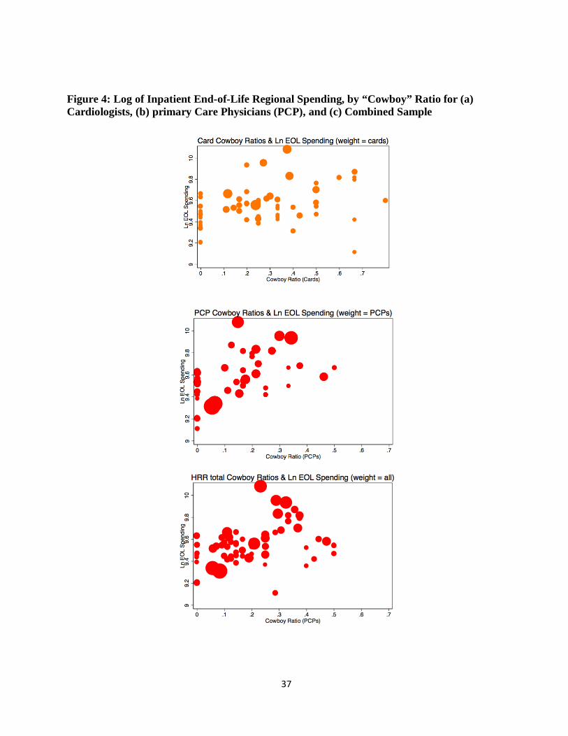
Column 1 of Table 3, the local proportion of cowboys and comforters predicts local spending
levels, explaining 38% of the regional variations in end-of-life spending in the sample after
controlling for local patient characteristics. The scatter plot showing the fraction of cowboy
physicians by HRR is shown in Figure 4 for the combined sample, as well as the individual
measures for either cardiologists, and for the primary care physicians. (The size of the dots are
related to the sample size in each HRR.) Additional regression results separately for cardiologists
and primary care physicians are also presented in Appendix Tables 1 and 2.
As Column 2 of Table 3 shows, recommended follow-up frequency is also a meaningful
predictor of HRR-level spending. (As noted above, we define “high follow up” physicians as
those whose recommended follow up frequency for a patient with hypertension (primary care 18 The final vignette, for Patient D, was only present in the cardiologist survey and not in the PCP survey. For this patient, who has a typical clinical presentation of new onset angina - pain or pressure in the chest arising with exertion – reasonable clinicians can differ with regard to a more- or less-intensive treatment protocol, and find justification in the literature for doing so. Furthermore, physician opinion\n regarding this patient did not predict regional spending patterns, only cardiac intervention rates.
22
physician) or stable angina (cardiologists) more than one standard deviation above the sample
average.) Knowing only these three supply-side preferences can explain 58% of the observed end-
of-life spending variation in our 64 HRRs. Figure 5 shows a scatter plot of predicted vs. actual
end-of-life spending according to this specification of the model with only supply-side factors.
This finding does, however, beg another question: is there an interaction effect that
emerges as a result of having a high proportion of multiple actors who are either aggressive or
comfort-prioritizing? (This interactive effect arises in the second term on the right-hand side of
Equation 6.) Specifically, we consider three possible 2-way interactions between the fraction of
primary care physicians, cardiologists and patients with aggressive preferences, shown in Table 4.
We then consider the three possible 2-way interactions between the fraction of primary care
physicians, cardiologists and patients with preferences for patient comfort and low-intensity
interventions – i.e. palliative care. Of these six possible interactions, we only find statistically
meaningful coefficients for the interaction between a high fraction of “comforter” primary care
physicians and a high fraction of patients with a preference for palliative care. In all other cases,
we fail to reject the null that the coefficient on the interaction term is zero and the primary result
above – namely that the local fraction of “cowboys,” “comforters,” and the fraction of “high
follow-up physicians” are strong and robust predictors of end-of-life spending in our sample. We
interpret this result as follows: when patients actually want less intensive care, the comfort-
prioritizing primary care physicians are the ones who try to accommodate patient preferences.
In a hypothetical world in which all physicians were comforters rather than cowboys, and
were below-average with regard to follow-up visits, the implied reduction in the log of end-of-life
inpatient expenditures would be 0.43, which is at least indicative of the degree of potential waste
in U.S. healthcare. Of course, these estimates are based on rather small samples of physicians and

23
patients across HRRs, but measurement error on the right-hand side of equations tends to
attenuate estimated coefficients.
What factors predict physician responses to the vignettes?
Here we estimate the model in Equation (2) using the physician data to test our hypotheses
as to the importance of a variety of financial and organizational factors. Specifically, we ask
which physician-level factors predict very aggressive, high utilization intervention
recommendations (i.e. being a “cowboy”) as well as which physician-level characteristics predict
lower intensity care recommendations (i.e. being a “comforter”). We do this for cardiologists and
primary care physicians separately and also run a set of combined regressions in which both
physician surveys are pooled19. Tables 5 and 6 present the results of this analysis using least
squares regressions, although results are similar in probit or logistics models.
We first consider factors that predict which physicians will be “cowboys” in our sample
(Table 5). We find that physicians in solo or 2-person practices (practice type 1) are more likely to
be aggressive than physicians in single or multi-specialty group practices (practice type 2) or
physicians who are part of a group or staff model HMO or a hospital based practice (practice type
3). As noted earlier, however, the fraction of capitated patients a physician sees is, if anything,
positively associated with being a cowboy for primary care physicians (with positive but
insignificant coefficients for cardiologists and in combined models). One would expect the
precise opposite result if physicians – especially primary care physicians – were to make
treatment decisions so as to maximize income.
We also note that factors typically associated with skill and quality of care are negatively
associated with cowboy status among primary care physicians: both board certification and the 19 In combined regressions, we control for the fraction of cardiologists in the sample by HRR to adjust for secular differences between primary care physicians and cardiologists in making intervention recommendations.

24
number of days per week a physician spends seeing patients are negatively predictive of cowboy
status. That is, board-certified physicians who spend more time seeing patients are less likely to
be cowboys than their counterparts who are not board certified and/or spend fewer days per week
with patients; in the combined sample of physicians, the coefficient on being board certified
implies a roughly 8 percentage point decrease in the probability of being a cowboy.
For primary care physicians, we see that a physician’s self-reported responsiveness to
expectations (or willingness to make a referral when not clinically indicated) is a positive
predictor of cowboy status – when in doubt, send the patient to a specialist. So those more
willing to refer to a specialist, for example because they report that their “colleagues would do so
in the same situation” are also more likely to be cowboys. Lastly, with respect to factors that
predict aggressive recommendations, we note that the number of cardiologists per capita seems to
be positively predictive of cowboy status. This could be viewed as evidence for the existence of
classic “induced” demand; the greater the density of cardiologists, the greater the pressure to treat
less appropriate patients (e.g., Gruber and Owings, 1996).
We next turn to the factors that predict which physicians are “comforters” – i.e. what
factors predict cost-mitigating – and in this case, clinically appropriate – recommendations such
as palliative care? We see in Table 6 that the relationship between practice type and physician
type largely disappears. While there is some evidence from the combined sample that physicians
in single or multi-specialty group practices (practice type 2) are less likely to be comforters than
physicians in solo or 2-person practices (practice type 1) or physicians who are part of a group or
staff model HMO or a hospital based practice (practice type 3), this relationship does not follow
any pattern that can be related back to financial incentives.

25
The number of patient days per week measure is now positively correlated with comforter
status, with a large coefficient in the combined sample albeit a weaker result in the cardiologist
sample. Another analog can be seen in the relationship between per capital cardiologists: just as
more cardiologists per capita were associated with a higher probability of recommending very
intensive care, fewer cardiologists per capita are now associated with a greater probability of
recommending less intensive and more appropriate care.
While board certification is no longer a statistically significant predictor of being a
comforter in Table 6, expectations responsiveness among cardiologists is now positively, albeit
weakly, predictive of being a comforter. At the same time, a greater frequency of cardiologists per
100,000 population reduces the likelihood of the physician being a comforter, particularly in the
combined sample.
VI. Conclusion
While there is an increasing consensus on the existence of meaningful regional variations
in healthcare utilization in the U.S. (Skinner, 2012) and across many countries,20 there is much
less agreement about causes of such variations – do they arise from patient demand, or the supply
of healthcare treatments? In this paper, we first find that patient demand, as proxied by patients’
responses to a nationwide survey, has only a modest predictive association with regional
Medicare end-of-life treatment patterns. Second, we find, however, that individual physician
heterogeneity regarding treatment options can explain a substantial degree of regional variations
in utilization among the U.S. Medicare population, a result that is consistent with Sirovich et al.
(2008), Lucas et al. (2010), and Wennberg et al. (1997).
20 See for example the bibliography of variations across countries compiled by the Wennberg Collaborative; http://www.wennbergcollaborative.org/Publications.htm.

26
We also find that the traditional factors in supplier-induced demand models, such as the
fraction of patients paid through capitation (or on Medicaid), or the responsiveness to financial
factors, have a larger role in explaining equilibrium variations in utilization patterns.
Organizational factors such as accommodating colleagues help to explain some but not all
individual intervention decisions. But the largest factor explaining these regional variations
appears to be physician beliefs about the effectiveness of treatments that are orthogonal to
perceived organizational and financial factors. Our results are therefore consistent with Epstein
and Nicholson (2009), who find large variations in Cesarean Section surgical rates among
obstetricians within the same practice, even after adjusting for where the physicians trained.
One concern about the interpretation of the vignette responses as “overuse” is that they
may not reflect the true productivity of physicians (in the sense of Chandra and Staiger, 2007),
thus unfairly characterizing a given physician as a “cowboy” who may be particularly skilled in
the use of a specific procedure, and would in fact be far ahead of the then-current professional
American College of Cardiology/American Heart Association guidelines (Hunt et al., 2005). Yet
the subsequent 2009 updates showed no trend towards more aggressive care (Hunt et al., 2009),
and even these guidelines may lead to overtreatment: some of the standards are based on
physician consensus or based on randomized trials that are performed in academic settings where
complication rates of procedures are lower than in community hospitals (e.g., Wennberg, et al.,
1998).
Another possibility is that “cowboys” may be more aggressive along several dimensions;
they may be more likely to use aggressive treatments without clear benefits, but they may also be
more likely to avoid the underuse of effective care, as suggested in the treatment of cancer
(Landrum et al., 2008). That is, physicians who are more likely to have their patients come back

27
more often for visits are also more likely to provide the high-value low-cost treatments. While we
cannot test this hypothesis directly, since we did not ask directly about “effective” treatments,
there is some evidence that overall end-of-life expenditures are at best poorly correlated with
health outcomes (Silber et al., 2010; Fisher and Skinner, 2010), and at worst not associated or
even negatively associated with outcomes and effective care (Baicker and Chandra, 2004; Fisher
et al., 2003a,b).
High rates of utilization may also arise because of the fear of malpractice. This might be
more plausible in the case of revisit rates, where physicians would be worried that some adverse
outcome may happen before the next visit. Yet sins of omission (as opposed to sins of
commission) are less likely to be a key consideration for the types of patients described in
Vignettes B and C, particularly where guidelines exist. Nor did malpractice concerns did not
predict the use of interventional stenting in our fourth vignette (not reported) of a patient with
new onset of chest pains.
While we document the importance of physician beliefs in explaining regional utilization
patterns, we have not suggested how such beliefs might have arisen. Simple heterogeneity in
physician beliefs cannot explain regional variation in expenditures, since in sufficiently large
regions, random differences in physician beliefs will cancel out; one requires spatial correlation in
beliefs to explain regional variations across a large number of physicians. We do find that
physicians’ propensity to intervene for non-clinical reasons is related to the expectations of
physicians with whom they regularly interact, a result consistent with Burke et al (2006) who
show that network and peer effects models can naturally lead to such spatial correlations. But we
are still left with a question of why some regions because become more aggressive than others,

28
and why such characteristics could be related to factors such as social capital (Skinner and
Staiger, 2007).
We do not mean to imply that economic incentives are unimportant. Clearly, changes in
payment margins will have a large impact on behavior, as in Clemens and Gottlieb (2012). But in
a system where the effects of price margins and reimbursement rates are blunted, physician
beliefs have a much larger scope to drive equilibrium variation in healthcare systems, particularly
for medical conditions where there is some uncertainty about the value of medical treatments or
where (in our case) guidelines are not always followed (McPherson et al., 1981, Wennberg and
Gittelsohn, 1975). In sum, our results point to an important role for physician beliefs in
explaining regional variations in utilization rates for treatments that may yield little value at the
margin.

29
REFERENCES Ameriks, John, Andrew Caplin, Steven Laufer, and Stijn van Nieuwerburgh, “The Joy of Giving or Assisted Living? Using Strategic Surveys to Separate Public Care Aversion from Bequest Motives,” Journal of Finance, 66(2), April 2011. Anthony, D. L., M. B. Herndon, P. M. Gallagher, A. E. Barnato, J. P. Bynum, et al., 2009, How much do patients' preferences contribute to resource use?, Health Aff (Millwood) 28, May-Jun, 864-73. Appleby, John, Veena Raleigh, Francesca Frosini, Gwyn Bevan, Haiyan Gao, et al., 2011. Variations in health care: The good, the bad and the inexplicable (The Kings Fund, London). Baicker, K., and A. Chandra, 2004. “Medicare spending, the physician workforce, and beneficiaries' quality of care,” Health Aff (Millwood) Apr 7. Baicker, Katherine, Kasey S. Buckles, and Amitabh Chandra, 2006, Geographic variation in the appropriate use of cesarean delivery, Health Affairs 25, w355-w367. Baicker, Katherine, Elliott S. Fisher, and Amitabh Chandra, 2007, Malpractice liability costs and the practice of medicine in the medicare program, Health Affairs (Millwood) 26, May-Jun, 841-52. Baker, L. C., E. S. Fisher, and J. E. Wennberg, 2008, Variations in hospital resource use for medicare and privately insured populations in california, Health Affairs 27, Mar-Apr, w123-34. Barnato, A.E, M.B. Herndon, D.L Anthony, P. Gallagher, JS Skinner, et al., 2007. “Are regional variations in end-of-life care intensity explained by patient preferences? A study of the US Medicare population,” Medical Care 45, 386-393. Baumann, Andrea O., Raisa B. Deber, Gail G. Thompson, 1991, “Overconfidence Among Physicians and Nurses: The ‘Micro-Certainty, Macro-Uncertainty’ Phenomenon,” Social Science and Medicine 32(1), 167-74. Black, William C., and H.G. Welch, “Advances in diagnostic imaging and overestimations of disease prevalence and the benefits of therapy,” NEJM 1993;328:1237-1243. Burke, Mary, Gary Fournier, and Kislaya Prasad, "The Emergence of Local Norms in Networks," Complexity, 11(5) May/June 2006: 65-83. Chandra, Amitabh, Jonathan Gruber, and Robin McKnight, 2010, Patient cost-sharing and hospitalization offsets in the elderly, American Economic Review 100, 193-213. Chandra, Amitabh, and Douglas O. Staiger. 2007. “Productivity Spillovers in Healthcare: Evidence from the Treatment of Heart Attacks,” J Political Economy 115, 103-140.

30
Chandra, Amitabh, and Jonathan Skinner, 2012, “Productivity growth and expenditure growth in U.S. Health care,” Journal of Economic Literature (September). Chen, Jersey, Sharon-Lise T. Normand, Yun Wang, and Harlan M. Krumholz, 2011. “National and Regional Trends in Heart Failure Hospitalization and Mortality Rates for Medicare Beneficiaries, 1998-2008,” JAMA, October 19, 306(15): 1669-78. Clemens, Jeffrey, and Joshua Gottlieb, 2012. “Do Physicians' Financial Incentives Affect Medical Treatment and Patient Health?” Stanford University (SIEPR), http://siepr.stanford.edu/publicationsprofile/2447. Colla, Carrie, Nancy E. Morden, Jonathan Skinner, J. Russell Hoverman, and Ellen Meara, 2012. “Impact of Payment Reform on Chemotherapy at the End of Life,” American Journal of Managed Care, 18(5 Spec No. 2): e200-e208. Connors AF, Jr, Dawson NV, Desbiens NA, et al. 1995: “A Controlled Trial to Improve Care for Seriously III Hospitalized Patients: The Study to Understand Prognoses and Preferences for Outcomes and Risks of Treatments (SUPPORT).” JAMA. 274(20):1591-1598. Dartmouth Atlas, 2012. www.dartmouthatlas.org . de Jong, Judith D., 2008. Explaining medical practice variation: Social organization and institutional mechanism (Nivel, Utrecht, The Netherlands). Doyle, Joseph, 2010, “Returns to local-area healthcare spending: Using shocks to patients far from home,” American Economic Journal: Applied Economics, 3(3): 221-43. Dresselhaus, Timothy R., John W. Peabody, Jeff Luck, Dan Bertenthal, 2004. “An Evaluation of Vignettes for Predicting Variation in the Quality of Preventive Care,” Journal General Internal Medicine, October; 19(10): 1013–1018. Timothy R Dresselhaus, MD,MPH,1,2 John W Peabody, MD,PhD,3,4,5 Jeff Luck, MBA,PhD,5,6,7 and Dan Bertenthal, MPH Epstein, Andrew J. & Nicholson, Sean, 2009. "The formation and evolution of physician treatment styles: An application to cesarean sections," Journal of Health Economics, 28(6): 1126-1140, December. (ESCAPE) Evaluation Study of Congestive Heart Failure and Pulmonary Artery Catheterization Effectiveness: The ESCAPE Trial. JAMA. 2005; 294(13): 1625-1633 Fisher, E. S., D. E. Wennberg, T. A. Stukel, D. J. Gottlieb, F. L. Lucas, et al., 2003a, The implications of regional variations in medicare spending. Part 1: The content, quality, and accessibility of care, Ann Intern Med 138, Feb 18, 273-87.

31
Fisher, E. S., D. E. Wennberg, T. A. Stukel, D. J. Gottlieb, F. L. Lucas, et al., 2003b, The implications of regional variations in medicare spending. Part 2: Health outcomes and satisfaction with care, Ann Intern Med 138, Feb 18, 288-98. Fisher, Elliott, and Jonathan Skinner, 2010. “Comment on Silber et al.: Aggressive Treatment Styles and Surgical Outcomes, Health Services Research 45: 1908-11 (December). Gruber, J., and M. Owings. 1996. Physician financial incentives and cesarean section delivery. Rand Journal of Economics 27 (1):99-123. Tamara B. Horwich, Tamara B, W. Robb MacLellan, and Gregg C. Fonarow, 2004. “Statin Therapy Is Associated With Improved Survival in Ischemic and Non-Ischemic Heart Failure,” Journal of the American College of Cardiology 43(4): 642-48. Hunt, Sharon Ann, William T. Abraham, Marshall H. Chin, Arthur M. Feldman, Gary S. Francis, et al., 2005. “ACC/AHA 2005 Guideline Update for the Diagnosis and Management of Chronic Heart Failure in the Adult: A Report of the American College of Cardiology/American Heart Association Task Force on Practice Guidelines (Writing Committee to Update the 2001 Guidelines for the Evaluation and Management of Heart Failure): Developed in Collaboration With the American College of Chest Physicians and the International Society for Heart and Lung Transplantation: Endorsed by the Heart Rhythm Society,” Circulation. 2005;112:e154-e235; (September 13). Hunt, Sharon Ann, William T. Abraham, Marshall H. Chin, Arthur M. Feldman, Gary S. Francis, et al., 2009. “2009 Focused Update Incorporated Into the ACC/AHA 2005 Guidelines for the Diagnosis and Management of Chronic Heart Failure in the Adult: A Report of the Amercian College of Cardiology Foundation/American Heart Association Task Force on Practice Guidelines: Developed in Association with the International Society for Heart and Lung Transplantation,” Circulation 119:e391-e479 (March 26). Jacobson, Mireille, A. James O’Malley, Craig C. Earle, Juliana Pakes, Peter Gaccione and Joseph P. Newhouse, 2006. “Does Reimbursement Influence Chemotherapy Treatment For Cancer Patients?” Health Affairs, 25(2): 437-443. Landrum, Mary Beth, Ellen R. Meara, Amitabh Chandra, Edward Guadagnoli and Nancy L. Keating, “Is Spending More Always Wasteful? The Appropriateness of Care and Outcomes among Colorectal Cancer Patients,” Health Affairs 27(1):159-168 (January). Levine-Taub, Anna A., Anna A. Levine Taub, Anton Kolotilin, Robert S. Gibbons, Ernst R. Berndt, “The Diversity of Concentrated Prescribing Behavior: An Application to Antipsychotics,” NBER Working Paper No. 16823 (February 2011). Lucas, FL, Siewers, AE, Malenka, DJ, Wennberg, DE. Diagnostic-therapeutic cascade revisited. Coronary angiography, coroabnry artery bypass surgery, and percutaneous coronary intervention in the modern era. Circulation. 2008;118:2797-2802.

32
McClellan, Mark, and Jonathan Skinner, 2006, “The Incidence of Medicare,” Journal of Public Economics 90, 2006/1, 257-276. McGuire, Thomas C., 2011, Physician agency and payment for primary medical care, in Sherry Glied, and Peter C. Smith, eds.: The Oxford handbook of health economics (Oxford University Press). McGuire, T.G., Pauly, M., 1991. “Physician response to fee changes with multiple payers.” Journal of Health Economics, 10 (4), 385-410. McPherson, Kim, PM Strong, Arnold Epstein, and Lesley Jones, 1981, Regional Variations in the Use of Common Surgical Procedures: Within and Between England and Wales, Canada, and the United States,” Social Science & Medicine. Part A: Medical Sociology 15 May, 273-88. Mandelblatt JS, Faul LA, Luta G, Makgoeng SB, Isaacs C, et al., 2012. “Patient and physician decision styles and breast cancer chemotherapy use in older women: Cancer and Leukemia Group B protocol 369901” Journal of Clinical Oncology July 20;30(21): 2609-14. Moliter, David, “The Evolution of Physician Practice Styles: Evidence from Cardiologist Migration,” MIT, 2011. http://economics.mit.edu/files/7301. National Health Service 2010. The NHS Atlas of variation in healthcare (November). http://www.rightcare.nhs.uk/atlas/qipp_nhsAtlas-LOW_261110c.pdf. Pauly, Mark, 1980. Doctors and their workshops: Economic models of physician behavior (University of Chicago Press, Chicago). Peabody JW, Luck J, Glassman P, Jain S, Hansen J, Spell M, Lee M., 2004. “Measuring the quality of physician practice by using clinical vignettes: a prospective validation study,” Annals of Internal Medicine Nov 16;141(10):771-80. Romley, J. A., A. B. Jena, and D. P. Goldman, 2011, Hospital spending and inpatient mortality: Evidence from california: An observational study, Annals of Internal Medicine 154: 160-7 (February 1). Rothberg, Michael B., Senthil K. Sivalingam, Javed Ashraf, Paul Visintainer, John Joelson, Reva Kleppel, Neelima Vallurupalli, Marc J. Schweiger, 2010. “Patients' and Cardiologists' Perceptions of the Benefits of Percutaneous Coronary Intervention for Stable Coronary Disease,” Annals of Internal Medicine (September). Silber, J. H., R. Kaestner, O. Even-Shoshan, Y. Wang, and L. J. Bressler, 2010, Aggressive treatment style and surgical outcomes, Health Serv Res 45: 1872-92 (December). Sirovich, B., P. M. Gallagher, D. E. Wennberg, and E. S. Fisher, 2008. “Discretionary Decision Making by Primary Care Physicians and the Cost of U.S. Health Care,” Health Affairs 27, May-Jun, 813-23.

33
Skinner, Jonathan, 2012. “Causes and Consequences of Geographic Variation in Health Care” in T. McGuire, M. Pauly, and P. Pita Baros (eds.) Handbook of Health Economics Vol. 2, North Holland. Skinner, Jonathan, and Douglas O. Staiger, 2007, Technological diffusion from hybrid corn to beta blockers, in Ernst Berndt, and Charles M. Hulten, eds.: Hard-to-measure goods and services: Essays in honor of Zvi Griliches (University of Chicago Press and NBER, Chicago). Skinner, J., D. Staiger, and E. S. Fisher, 2010, Looking back, moving forward, N England Journal of Medicne 362: 569-74 (February 18). Skinner, Jonathan, and Douglas Staiger, 2009, Technology diffusion and productivity growth in health care, Working Paper Series (National Bureau of Economic Research, Cambridge MA). Suleman M, Clark MP, Goldacre M, Burton M., 2010. “Exploring the Variation in Paediatric Tonsillectomy Rates between English Regions: a 5-year NHS and Independent Sector Data Analysis. Clin Otolaryngol. 2010 Apr;35(2):111-7. Wennberg, David E., et al. 1998. “Variations in Carotid Endarterectomy Mortality in the Medicare Population: Trial Hospitals, Volume, and Patient Characteristics.” JAMA, 279(16): 1278-81. Wennberg, John E., 2010. Tracking medicine: A researcher's quest to understanding health care (Oxford University Press, New York). Wennberg, John E., and Alan Gittelsohn, 1975. “Health Care Delivery in Maine I: Patterns of Use of Common Surgical Procedures,” The Journal of the Maine Medical Association 66(5): 123-130 & 149 (July). Wennberg, David E; Kellet, MA; Dickens, Jr., JD; Malenka, DJ; Keilson, LM; Keller, RB: The Association Between Local Diagnostic Testing Intensity and Invasive Cardiac Procedures. JAMA, Vol. 275, No. 15; p1161-1164; April 17, 1996. Wennberg, David E; Dickens, Jr., JD; Biener, L; Fowler, Jr., FJ; Soule, DN; Keller, RB., 1997. “Do Physicians Do What they Say? The Inclination to Test and Its Association with Coronary Angiography Rates.” Journal of General Internal Medicine 12(3):172-176. Wennberg, John E., Elliott S. Fisher, and Jonathan S. Skinner, 2002, Geography and the debate over medicare reform, Health Affairs Web (www.healthaffairs.org), W96-W114. Zuckerman, S., T. Waidmann, R. Berenson, and J. Hadley, 2010. “Clarifying Sources of Geographic Differences in Medicare Spending.” New England Journal of Medicine 363 (1):54-62.

34

35
Figure 1: Diagram of Reasons Why Variations Exist in Equilibrium: Differences in λ and Differences in Actual or Perceived Productivity
Ψg′(x)
Ψs′(x)

36
Figure 2: Fraction of Patient Who Would See Unneeded Cardiologist (HRR-Level Distribution)
Figure 3: Distribution of Length of Time before Next Visit for Patient with Well-Controlled Angina (Cardiologist HRR-Level Distribution)
37
Figure 4: Log of Inpatient End-of-Life Regional Spending, by “Cowboy” Ratio for (a) Cardiologists, (b) primary Care Physicians (PCP), and (c) Combined Sample

38
Figure 5: Predicted and Actual Log End-of-Life Expenditures (Combined Weights)