phys%575% autumn%2015 radia&on!and!radia&on!detectors!
TRANSCRIPT
PHYS 575 Autumn 2015
Radia&on and Radia&on Detectors
Course home page: h6p://depts.washington.edu/physcert/radcert/575website/
R. Jeffrey Wilkes Department of Physics
B305 Physics-‐Astronomy Building 206-‐543-‐4232
5: cross sec&ons, a6enua&on; calorimetry; coun&ng sta&s&cs; sta&s&cs for analysis

Course calendar
2
Tonight

Announcements
• Send me your report proposal! topic, brief summary, list of proposed resources/references
• PresentaRon dates: Tues Dec 1, Tues Dec 8, and Thurs Dec 10 – See class web page for link to signup sheet
– Volunteers needed for early slots (Dec 1) – I will arbitrarily assign slots for those not signed up by November 29
10/27/15 3

10/27/15 4
Cross secRons and accceptance First: Ω = solid angle acceptance of detector:
Project an element of detector area as viewed from source onto a 1m radius sphere:
Total cross secRon σ = Nevents / (Δt Ntgt Ibeam) Ibeam =( Nbeam /Δt ) / ΔS for beam area ΔS larger than
target, parRcles/cm2/sec Ntgt = number of target nuclei in beam area (or number of electrons in beam, for Compton sca_ering)
=(Navogodro Mtgt /Atgt )Ztgt (Mtgt in moles) σ has dimensions of area, unit : barn = 10-‐28 m2
Can have various parRal differenRal cross secRons: vs energy = dσ/dE vs angle = dσ/dθ vs several things at once: eg, d3σ / dE dθ dΩ
= cross secRon at energy E (per unit E) and angle θ (per unit θ), per unit solid angle dΩ centered on θ
area under dσ/d(whatever) curve = σ
10/27/15 4
R=1m
dA1 dA
ΔΩ source
detector
Beam
ΔS
target
total cross secRon for that process

Cross secRons
10/27/15 5
Partial differential cross sections From 1988 Int. Conf. on HEP (UA1 experiment reports)

A_enuaRon length • A_enuaRon length:
In terms of flux Φ (parRcles per cm2 in beam) vs depth, Simple differenRal eqn. which has soluRon
• A_enuaRon coefficient:
– So µ = nσ = 1/λ Mass a_enuaRon coefficient:
6
n = number density of targets in 1/cm-3 z = thickness in g/cm2 ns = 1/λ, attenuation length in cm

Collisions: impact parameter • Impact parameter b
Distance between target center and beam parRcle in individual collision – Example: Rutherford sca_ering: he found where Θ = (plane) sca_ering angle b = distance of closest approach to nucleus à effec)ve nuclear radius r Classical physics says: for electrostaRc force, acRng on projecRle with charge q1, mass m and speed v, near charge q2. So Rutherford found b~ 3x10-‐14 m for gold
(actually: rGOLD ~ 7x10-‐15 m -‐-‐ he used low energy alphas)
7

A_enuaRon and shielding for gammas • “Good geometry” arrangement
– Limited angular range for gammas from source • Sca_ered gammas are not counted: only survivors w/o interacRon • Disappearance of gammas is simple sum of probabiliRes
(photoelectric absorpRon) + (compton) + pair producRon
• Can define linear a_enuaRon coefficient µ: I = I0 exp(-‐ µ t)
• Mass a_enuaRon coeff = µ/(absorber density ρ) = cm/g2 • For absorber = mixture of materials, use weighted sum of MAC’s
10/27/15 8
I0 = source intensity, t = absorber thickness, µ = a_enuaRon coeff. (cm-‐1)
Dwg from http://www.nucleonica.net/wiki/
10/27/15 9
From: C. Melcher, Industrial applications of scintillators
Example: rotating scanner for inspecting pipe wall uniformity
“good-geometry” setup
10/27/15 10
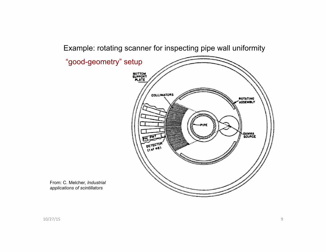
ElectromagneRc cascade development
• Electron entering dense ma_er soon brems (mean free path ~X0) • Brem photon soon pair-‐produces (mfp ~ (7/9)X0)
– etc, etc: result is a cascade or shower of electrons and photons – Number of parRcles builds up (and <E> per parRcle diminishes) unRl <E>~ECRITICAL
• Then brem losses become less important than ionizaRon
• NoRce brem/PP cascade process does not dissipate energy, just swaps it from e’s to photons and back again
• Main effect: divide energy up among more and more parRcles
• Cascade growth stops when average energy is too small to convert (less than EC)
• Energy is lost to medium (heaRng) only via ionizaRon, ater e’s drop below EC
(Only particles with E>1.5 MeV are counted)

ElectromagneRc cascade process
10/27/15 11
Photo from MIT cosmic ray group 1938

EM showers in detector design • EM “calorimetry”
– Basic way to measure energy of electrons or gammas • Thick absorber interleaved with parRcle counters • Number of parRcles vs depth and compare to calculaRons
– can esRmate total E of incoming e or gamma energy to O(10%)
– Ideal = “Total absorpRon calorimeter” – nothing escapes – Real = truncated shower measurement with “punch-‐thru” – Tools
• GEANT = parRcle physics industry standard for detector simulaRon • EGS = code developed at Stanford for cascade simulaRon
• Hadronic calorimeters – Same idea, but for protons/nuclei: much more complicated process! Much more depth needed.
10/27/15 12

Other cascade effects to consider
10/27/15 13
C. Crannell et al, PRL 182:1432 (1969) • Radial distribuRon of shower parRcles – Most parRcles in narrow core
• TransiRon effect: – Rapid change in relaRve
populaRons of e’s and gammas when Z changes
– TransiRon radiaRon = x-‐ray photons produced at interface
– TransiRon radiaRon detector (TRD) =
• exploit TR to measure cascade
• Very thin layers of Pb and plasRc, use x-‐ray detector below many layers

TransiRon radiaRon/calorimeter • Example: NOE’ detector (INFN/Naples, Italy)
www1.na.infn.it/wsubnucl/accel/noe/noe.html
Setup in CERN beam
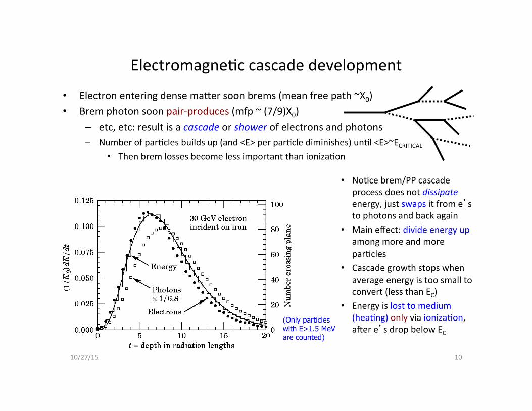
Example of calorimeter • Total absorpRon calorimeter for protons
– Proton interacts with nucleus producing mesons • Mesons interact again, or decay to electrons, photons, muons
– Count charged parRcles present, at intervals in absorber • Area under plot of number vs depth = EsRmate of total track length of shower parRcles in absorber
• (Total track length)(energy loss per track per cm at criRcal energy) à esRmate of total energy deposited by incoming proton
Underestimates E0 due to: • “Punch-through” =
remnant of shower that escapes through bottom
• Neutrons and neutrinos are not observed
Use simulation studies to estimate missed energy

• Individual proton events show large fluctuaRons – Nuclear interacRons inject many mesons, photon cascades have shorter length than
overall hadron-‐electromagneRc cascade • Average curves from many events + simulaRons can be used to calibrate
Individual showers and average showers
Area under curve à estimate of total track length T Assume most tracks are around critical energy, then
E0 ~ T Ec

10/27/15 17 10/27/15
CounRng experiments and staRsRcs • Coincidence measurements
– Simultaneous signals from two or more detectors (eg scinRllators) define events of interest
• Must define what we mean by “simultaneous” (window width) • Must define “interesRng” (coincidence pa_ern / logic)
– Coincidence circuits (= logical .AND.) • Simple coincidence (channel 1 .AND. Ch 2 . AND. Ch 3…) • “Majority logic”: any n-‐fold subset of all inputs
– Eg, 2-‐fold for 3 inputs = (1 and 2) or (2 and 3) or (1 and 3) • Include possibility of veto (.NOT. or logical inversion) for inputs (Ch 1 . AND. Ch 2 . AND.(.NOT.Ch 3) )
– Must first convert raw PMT output to logic pulse: discriminator circtuit (one-‐shot)
• Variety of analog pulses -‐> standardized logic signal – Specify voltage level (threshold) to trigger discriminator
• Set output of the discriminator to a fixed height (choice of industry standard: TTL, NIM, etc), and duraRon (width)
• Q: how do we know counts are meaningful?
17
10/27/15 18
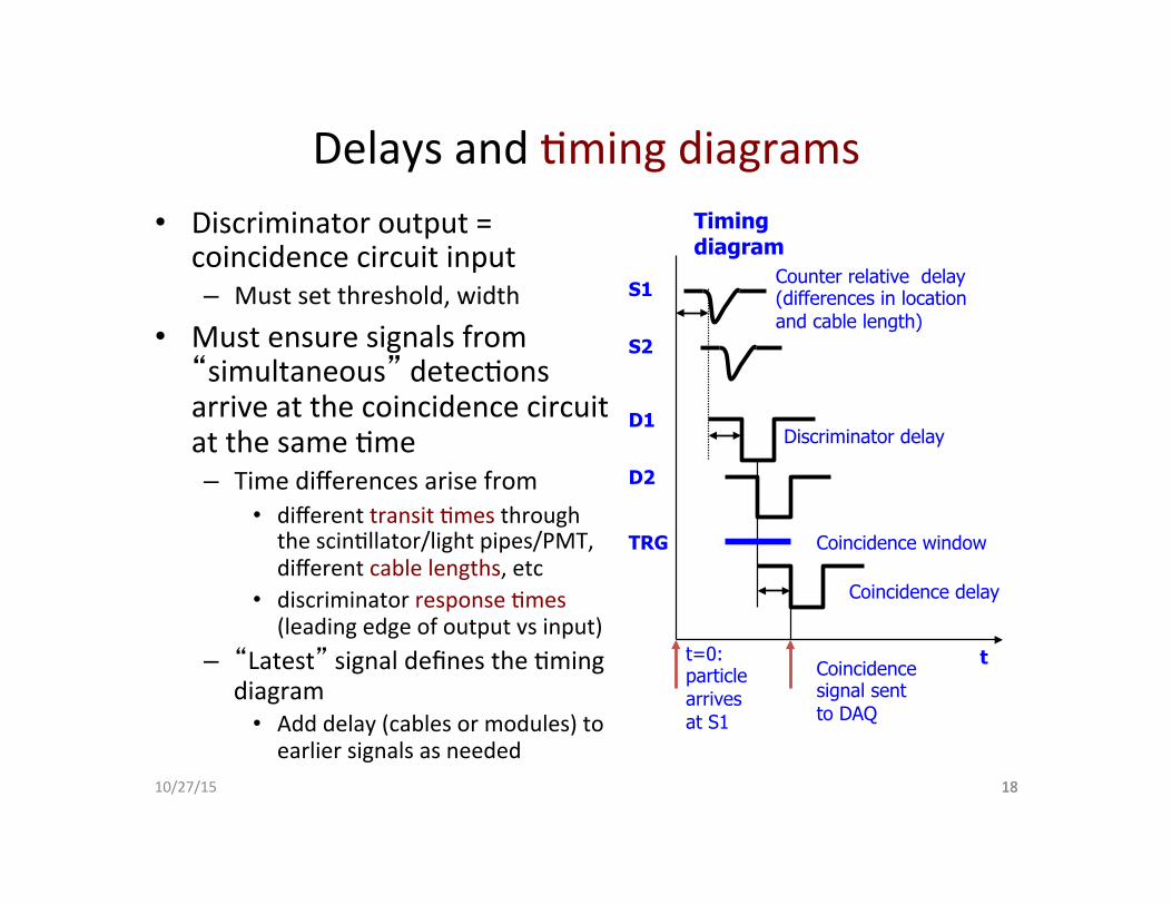
Delays and Rming diagrams • Discriminator output =
coincidence circuit input – Must set threshold, width
• Must ensure signals from “simultaneous” detecRons arrive at the coincidence circuit at the same Rme – Time differences arise from
• different transit Rmes through the scinRllator/light pipes/PMT, different cable lengths, etc
• discriminator response Rmes (leading edge of output vs input)
– “Latest” signal defines the Rming diagram
• Add delay (cables or modules) to earlier signals as needed
18
t
S1
S2
D1
D2
TRG
Timing diagram
t=0: particle arrives at S1
Counter relative delay (differences in location and cable length)
Discriminator delay
Coincidence delay
Coincidence window
Coincidence signal sent to DAQ

DeadRme and Accidental coincidences • Random signals from counters may fall within the coincidence Rme window
and create an accidental count – Uncorrelated background parRcles happen to arrive simultaneously – Random noise from PMT, or ambient electronic noise
• To esRmate the rate of accidental coincidences we need to know the resolving Rme of the system: minimum )me difference – Depends on width of pulses input to the coincidence circuits, and the singles rate
from each detector – Resolving Rme is measured by delaying one signal with respect to the other and
plo{ng the coincidence counts per unit Rme (delay curve) • Set delay between counters to where delay curve is max
• If N1 and N2 are the singles rates and σt the resolving Rme, then the accidental rate will be approximately NA = σt N1 N2 – σt N1 = Rme coincidence input 1 is on; N2 = opportuniRes for an accidental
• Other factors affecRng coincidence efficiency – DeadRme = Rme ater detecRon when detector cannot generate a new signal – Ji_er (random fluctuaRon) in Rming of counter signal relaRve to parRcle arrival 10/27/15 19

CounRng staRsRcs • Generally, we need to esRmate probability of interesRng events from a
staRsRcal sample of data: Recall:
– StaRsRc = single number, derived from data alone, describing some feature of a large data sample
– Probability distribuRon = relaRve likelihood of different sample values Some sample variables are integers (eg, counts); others are real-‐valued. For f(x) dx = Probability( x will be found in range {x→x+dx} ) (with f(x) properly normalized to give ∫all xf(x)dx = probability of any x =1) • f(x) = Probability Density Func)on (PDF)
– “differenRal probability distribuRon” x • F(x) = ∫-‐ ∞ f(x)dx = Cumula)ve probability distribuRon
– “integral distribuRon” F(-‐ ∞)=0 and F(+ ∞)=1; F is monotone increasing with x
• EsRmate PDFs by making a histogram of experimental results (limited samples of x) histogram = bar graph of number of occurrences vs x N(Δx) = Ntotal f(x) Δx → f(x) ~ N(Δx)/(Ntotal Δx)

00.020.040.060.080.10.12
-3 -2 -1 0 1 2 3
x
p(x)
P(x<0) P(x)dx
• PDF p(x)=probability of x in range x’ to x’+dx
• “Probability distribuRon” P(x)=(cumula)ve or integral distribuRon) =probability of x<x’
))()( ∞= ∫ - be could (where MIN
x
x
xdxxpxPMIN
0
0.250.5
0.75
1
-3 -2 -1 0 1 2 3
x
P(x)
Normal (Gaussian) PDF
Cumulative Standard Normal distribution
(erf(x)=“error function”)
21( ) exp( )22xp x
π= −
12
( ) 1 erf2xP x
⎡ ⎤⎛ ⎞= +⎢ ⎥⎜ ⎟
⎝ ⎠⎣ ⎦

Examples of distribuRons and histogram • Table = list of data, binned in x
– Simulated sample of 1000 events – Histogram = plot of table
• Curves = plots of underlying probability distribuRons – Black = PDF used to generate data sample: Gaussian centered on x=3 – Pink = cumulaRve Gaussian probability (P(ge{ng any value < x) )
x Frequency Cumulative %-5 0 0%-4 0 0%-3 1 0%-2 2 0%-1 11 1%0 52 7%1 95 16%2 156 32%3 191 51%4 171 68%5 156 84%6 85 92%7 61 98%8 13 99%9 6 100%
10 0 100%
Gaussian, mean=3, sigma=2histo = 1000 samples
curve = exact
0
50
100
150
200
250
-5 -3 -1 1 3 5 7 9 11More
Freq
uenc
y
0%
20%
40%
60%
80%
100%

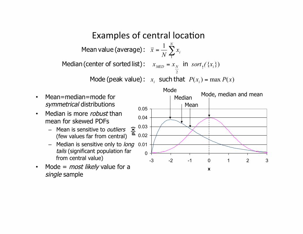
DescripRve parameters for PDFs Commonly used sta)s)cs: • Measures of central locaRon:
mean <x> = Σ xi / N (sample mean) median = x at which F(x)=0.5 mode = x at which f(x)=maximum for symmetrical distribuRons, mean=median
• Measures of width of distribuRons: variance σ2 ( σ = standard devia)on) σ2 = Σ(xi -‐ µ1 )2 / N but µ1 = mean of true PDF we can only es)mate µ1 with <x> Best esRmator for σ2 is s2 = Σ(xi -‐ <x>)2 / (N -‐1) = sample variance
• Central moments: devia)on from mean di = xi -‐ <x> <d n> = µn = nth central moment (average of di n )
µn = ∫all x (x-‐ µ1 )n f(x) dx eg, n = 3 (skewness) gives measure of asymmetry, etc
Binomial distribution
00.050.10.150.20.250.3
0 2 4 6 8 10
N
P(N
)
Central location
Width
Examples of central locaRon
)(max)(
}){
1
2
1
xPxPx
x(sortxx
xN
x
ii
iNMED
N
i
=
=
=
↑
∑
that such : value)(peak Mode
in :list) sorted of(center Median
:(average) valueMean
0
0.01
0.02
0.03
0.04
0.05
-3 -2 -1 0 1 2 3
x
p(x)
Mode Median
Mean
Mode, median and mean • Mean=median=mode for symmetrical distributions
• Median is more robust than mean for skewed PDFs
– Mean is sensitive to outliers (few values far from central)
– Median is sensitive only to long tails (significant population far from central value)
• Mode = most likely value for a single sample

• Example of an asymmetrical distribuRon: World per capita income distribuRon (for 1993)
– A small percentage of people have very large incomes, relaRvely – Mean = poor esRmate of central value for highly skewed PDF
• Long tail “pulls” the average value up
World Per Capita Annual Income 1993
0
0.02
0.04
0.06
0.08
0.1
0 1000 2000 3000 4000 5000
US$
Perc
ent o
f pop
ulat
ion
Mean = $3600
Median = $1044
Measures of central locaRon
Mode = $400

Measures of distribuRon width
00.0050.010.0150.020.0250.030.0350.040.045
-3 -2 -1 0 1 2 3
x
p(x)
± a
± σ
HWHM FWHM
a σ
• Variance:
– Popula)on variance: Use N if we somehow know the mean value a priori – Note that mean and variance are 1st and 2nd moments of PDF – Variance has special significance in staRsRcs (more later)
• Standard deviaRon: σ=√σ2 – Most commonly used measure of width
• Mean absolute deviaRon: – Not oten useful
• Full-‐ or Half-‐Width at half maximum (FWHM/HWHM) – Commonly used in engineering
x
xxN
N
ii
find to the used webecause 1-N Use : is this
)(1
1 2
1
2
set data same
variance sample
∑=
−−
=σ
∑=
−=N
ii xx
Na
1
1

Famous probability distribuRons • Uniform distribuRon
– Only PDF generator available on all computer systems • Can construct all others from this (more later)
0
0.25
0.5
0.75
1
-0.25 0 0.25 0.5 0.75 1 1.25
x
f(x)
a b µ 0
1
p(x)
P(<x)
)(21)(
)()()()(
)()(
1)(
badxxpx
abaxdxxpxP
bxaab
xp
b
a
x
a
+==
−
−==<
≤≤−
=
∫
∫
µ
σ
1.2- kurtosis 0, skewness )(small! 1215.0 :1-0 rangefor e.g.,
)(121)()(
2
222
====
−=−= ∫
σµ
µσ abdxxpxb
a
Binomial distribution
00.050.10.150.20.250.3
0 2 4 6 8 10
N
P(N
)
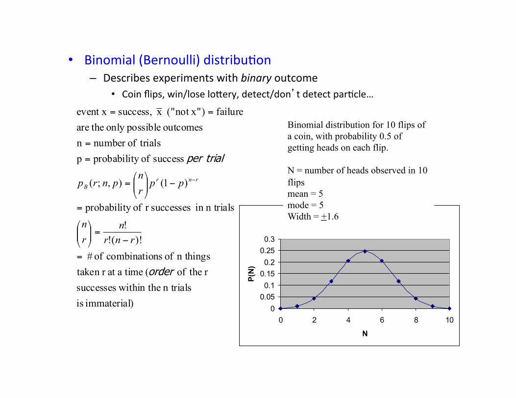
• Binomial (Bernoulli) distribuRon – Describes experiments with binary outcome
• Coin flips, win/lose lo_ery, detect/don’t detect parRcle…
)immaterial is n trials e within thsuccesses
r theof ( timeaat r taken n things of nscombinatio of #
)!(!!
n trialsin successesr ofy probabilit
)1(),;(
success ofy probabilitp trialsofnumber n
outcomes possibleonly thearefailure)not x"(" x success,event x
order
trial per
=
−=⎟⎟
⎠
⎞⎜⎜⎝
⎛
=
−⎟⎟⎠
⎞⎜⎜⎝
⎛=
=
=
==
−
rnrn
rn
pprn
pnrp rnrB
Binomial distribution for 10 flips of a coin, with probability 0.5 of getting heads on each flip. N = number of heads observed in 10 flips mean = 5 mode = 5 Width = +1.6

ApplicaRons of binomial distribuRon Contents of a single bin in a histogram (n total entries) Common assumption: Poisson limit (for small p: more on this later)
0
20
40
60
80
100
1 6 11 16 21 26 31 36
x
N(x)
2
ˆ ,
ˆ ) 1(1
ˆ ˆ ˆ(1 ) 1
1
x x p xrp rn
rso pn
q
rnpq n p p rn
rr rn
σ
σµ
= = =
= =
= −
⋅ ⋅
= −
⎛ ⎞= = − = −⎜ ⎟⎝ ⎠
⎛ ⎞± = ± −⎜ ⎟⎝ ⎠
inside bin, outside probability of
From the data, we estimate contents of bin
r=σ
here: r=67, n=1000, so p=.066, σ=7.9
22
2 2
( , ) ( , ) (1 ),B B
rrn
p (r;n p) p (r;n p)np npq p ppn n n n n
µ σµ σ
→
−→ = = → = =
Note : Event counts are but efficiencies are numbers
Change variable to frequency :
integers, real
relative

Poisson distribuRon • LimiRng case for binomial distribuRon with p
small and n large – p → 0 and n → ∞ such that (np) ~ constant
nppp
er
rppnrp
BP
rPB
=
→
→==→==
==→ −
µ
µ
µµσµσµ
µµ µ
:n largefor eapproximat to Use ; largefor on)distributi normal( lSymmetrica~
right the toalways tail1skewness , mean value
!1);(),;(
2
0
0.2
0.4
0.6
0.8
0 1 2 3 4 5
r
pP(r;µ)
m=0.2m=0.5
µ<1 ~ exp peak at 0
0
0.1
0.2
0.3
0.4
0 1 2 3 4 5 6 7 8
r
pP(r;µ)
m=1m=2
µ~1: peak appears
0
0.05
0.1
0.15
0.2
0 5 10 15 20 25 30r
p P(r;µ)
m=5m=10m=20N(20,4.5)
µ>>1: shape approaches Gaussian

ApplicaRons of Poisson distribuRon • NoRce pPOIS(r) is limited to r = integer only
– Value of µ (not necessarily integer) should be “small” – Range of r is bounded on the let (by r=0) – Approaches normal dist. for µ “large” (far from 0) – Has only one parameter: µ
• ApplicaRons – RadioacRve decay counRng data: µ = mean counts/sec Then prob. of r counts/sec is Example: suppose µ = 20 counts/sec Then prob of 30 counts in any one sec period is about 1% (~ same for 10 counts) – Bubbles in a bubble chamber track: µ = mean bubbles/cm: (or hits in any ionizaRon tracking detector: ionizaRon is proporRonal to Q2) Then prob. of ge{ng r bubbles/cm is given by Poisson distribuRon Example: suppose proton (Q=1) tracks have 9 bubbles/cm on average Searching 1000 pictures, a track is found with 1 bubble/cm -‐-‐ a quark (Q=1/3)? Prob that this is just a random fluctuaRon of a proton track? pp (20;9)=0.0011
so expect to see this with odds ~1:1000… Not unlikely enough! ("Discovery Threshold" is currently around P~10-‐4)
µµµ −= er
rp rP !
1);(

32
Poisson assumpRons • Physical situaRons where Poisson Assump)ons are valid lead to behavior
reflecRng the exponenRal and Poisson distribuRons: 1. p(1 event) in interval δx is propor)onal to δx: p=g δx 2. Occurrence of an event in some interval δxj is independent of events (or
absence of events) in any other non-‐overlapping interval δxk 3. For sufficiently small δx, there can be at most 1 event in δx – Examples: ionizaRon in a gas, goals scored in a soccer match, requests for documents
on a web server, radioacRve decays
• From these we can derive the exponenRal and Poisson distribuRons:
So exponen)al distribuRon = gap length distribuRon p0(x) between events in a
Poisson process (gaps in a bubble chamber track or ionizaRon trail)
Prob of 1 bubble in δ x : p1(δ x) = gδ x ( from #1)Prob of 0 bubbles in δ x : p0 (δ x) = 1− p1 = 1− gδ x ( from # 3)p0 (x + δ x) = p0 (x)• p0 (δ x) = p0 (x)(1− gδ x) ( from # 2)
∴p0 (x + δ x) − p0 (x)
δ x= −gp0 (x)→ dp0
dx= −gp0
Solution : p0 (x) = e−gx
Prob of exactly r bubbles in x + δ x :pr (x + δ x) = pr (x)• p0 (δ x) + pr−1(x)• p1(δ x) ( from # 3)
∴pr (x + δ x) − pr (x)
δ x→
dprdx
= −gpr (x) + gpr−1(x)
Solution : pr (x) = 1r!
(gx)r e−gx = Poisson (µ = gx)

ExponenRal distribuRon • Special case of frequent interest: probability of ge{ng exactly one event
under Poisson case: 1(1; )Pp e µµ µ −=
/
/
1
1
: ( ; )
: ( ; ) 1
t
t
PDF p t e
Cumulative P t e
λ
λ
λ
λ
λ
λ
−
−
=
< = −
0
0.1
0.2
0.3
0.4
0.5
0.6
0.7
0.8
0.9
1
0 0.5 1 1.5 2 2.5 3 3.5
p(x)P(x)
Example: radioacRve parRcle has mean life λ
Probability that parRcle decays within any Rme window of length t is given by cumulaRve exponenRal distribuRon (integral distribuRon)

N(0,1), N(0,2), N(0,3)
0
0.05
0.1
0.15
0.2
0.25
0.3
0.35
0.4
0.45
-3 -2 -1 0 1 2 3
Gaussian (“Normal”) probability density fn (PDF)
• Gaussian = famous “bell-‐shaped curve” – Describes IQ scores, number of ants in a colony of a given species, wear
profile on old stone stairs... All these are cases where: – deviaRon from norm is equally probable in either direcRon – Variable is conRnuous (or large enough integer to look conRnuous -‐ far from
the “wall” at n = zero) • Real-‐valued PDF: f(x) → -‐ ∞ < x < + ∞
n(x;µ,σ)= (1/sqrt[2πσ2]) exp[-‐(x-‐µ)2/2σ2 ] • 2 independent parameters: µ , σ (central locaRon and width) • ProperRes:
Symmetrical, mode at µ , median=mean=mode InflecRon points at ±σ Standard normalized form: scale x by σ , shit origin to µ n(x;0,1) = (1/sqrt[2π]) exp[-‐x2] CumulaRve distribuRon: N(x)= ∫-‐∞x n(x;0,1)dx = erf(x) Area within (prob. of observing event within) ± 1σ = 0.683 = erf(1)-‐erf(-‐1) ± 2σ = 0.955 = erf(2)-‐erf(-‐2) ± 3σ = 0.997 = erf(3)-‐erf(-‐3)
Binomial and Poisson distributions
00.020.040.060.080.10.120.140.160.180.2
0 10 20 30 40x
P(x
)
Mean=1
Mean=5
Mean=10 Mean=25
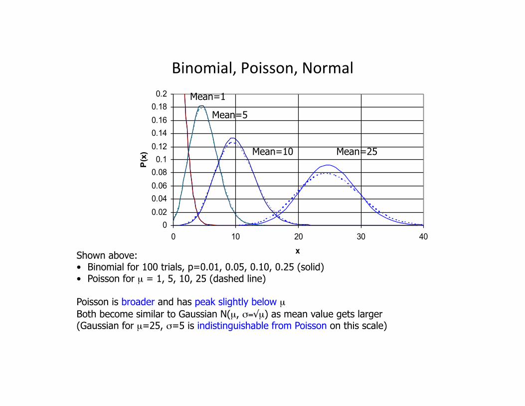
Shown above: • Binomial for 100 trials, p=0.01, 0.05, 0.10, 0.25 (solid) • Poisson for µ = 1, 5, 10, 25 (dashed line)
Poisson is broader and has peak slightly below µ Both become similar to Gaussian N(µ, σ=√µ) as mean value gets larger (Gaussian for µ=25, σ=5 is indistinguishable from Poisson on this scale)
Binomial, Poisson, Normal

36
Significance of normal distribuRon • Central Limit Theorem:
“Given N independent random variables xk, each with µk and σk specified (but not details of individual PDF’s), the random variable z = Σ xk has mean value µ = Σ µk and variance σ2 = Σ σk
2 and for large staRsRcs, its PDF will be Gaussian, ie
(Σ xk -‐ Σ µk ) / sqrt[Σ σk2 ] = n(x;0,1)”
• Applies to: any situaRon with real-‐valued result where several independent processes add: addiRve errors.
• Parameters µ,σ are independent (and converse: if a random variable has µ,σ independent, it is normal). Given N random numbers xk from a normal
distribuRon, the sample mean µ = (1/N)Σ xk and sample variance s2 = Σ σk
2 / (N-‐1) are independent sta)s)cs
ApplicaRon examples: • Random walk of 100 steps. Each step is independent of others, any probability distribuRon for direcRon and length of each step (but µ, σ2 known).
• To make a simple Gaussian random number generator, just take sum of 12 uniformly distributed numbers on [0,1):
x=Σ (uk -‐ 6); x will be distributed ~ n(x;0,1) (recall: uniform(0;1) has µ= 0.5, σ2= 1/12 )

37
Examples of normal distribuRons • Gain distribuRon for 11,000 photomulRplier tubes which are supposed to be
~idenRcal (from Super-‐K neutrino experiment) – Gain depends on many independent factors (tube manufacture batch, geometry,
power supply stability, cable characterisRcs...)
• GPS clock Rmes (again from Super-‐K, yesterday's data) – Time fit depends on many indep. factors (exact antenna locaRon, sotware design,
receiver characterisRcs...)

Special physics PDFs: Landau distribuRon
10/27/15 38
• Landau described the distribuRon of energy losses for parRcles passing through a thin layer of absorber • Long tail on the right, cut off sharply on the let -‐> most losses near
average, but big losses possible, and less infrequent than for Gaussian • Related to the Cauchy (Breit-‐Wigner) and Gaussian distribuRons
• Landau is a member of the Stable DistribuRon family, which includes Gaussian, Cauchy and Delta funcRons
See math.uah.edu/stat/special/Stable.html

Breit-‐Wigner distribuRon • B-‐W distribuRon describes distribuRon of energy seen in decays of very
short-‐lived states (resonances)
39
Example from CERN LHCb experiment, showing Upsilon meson (= b-anti-b quark pair) and 2 excited states, decaying promptly to muons. B-W shapes are fitted to excess over smooth random background counts in each bin lhcb-public.web.cern.ch
In parRcle physics units, where ħ = c = 1: E = center-‐of-‐mass energy of the decay products, M is the mass of the resonance (peak locaRon), Γ is the resonance width, and mean lifeRme τ = 1/Γ.

ApplicaRon of staRsRcs: hypothesis tesRng • Given
– 2 data samples: {xi=1…N}, {xj=1…M} OR – data sample {xi=1…N} and model f(x;θ)
• We want to test the “Null Hypothesis”: H0 : {xi=1…N} and {xj=1…M} are drawn from the same populaRon distribuRon [ alternaRvely: {xi=1…N} is drawn from f(x;θ) ] – “non-‐parametric tests” = no assumpRons made about the underlying
populaRon distribuRon
Chi-‐squared test (Pearson’s test) – Histogram the {xi} to esRmate differenRal dist. – ni = number of entries in bin i (xi < x < xi+δx), δx=histogram bin width – To test f(x):
BINSN largeor largefor correct is theoremlimit Central
of estimate Poisson isr Denominato
r)denominato in 0 ( binsempty excludemust :Note
integer)y necessarilnot is (
i
f
i
xix
ixi
N
i i
ii
n
m
dxxfmwheremmn
2
2
2
1
2 )(
χ
σ
χδ
→
=⎟⎟⎠
⎞⎜⎜⎝
⎛ −= ∫∑
+
=

41
Chi-‐squared Sampling distribuRons describe staRsRcs of data samples as a whole • Chi-‐squared distribuRon
– For example: if µ is unknown a priori, we must use average x as es)mator for μ:
χ 2 ≡(xi − µ)2
σ 2i=1
N
∑ summed deviations squared, in units of σ 2
p(χ 2;ν) = 12ν /2Γ(ν / 2)
(χ 2 )ν /2−1 exp(−χ 2 / 2)
= χ 2 PDF for ν degrees of freedomν = number of independent variables in sum
∑∑
∑
∑
==
−=
−=
−=−
−=→−
≡
=
=
=
M
i
M
ii
iM
N
ii
N
i
i
puw
uuuNp
snz
snxx
Npxx
1
22
1
221
2
22
2
2
1
2
2
12
22
);(
...,)1;(
)1(
)1()(
)1;()(
ννχχ
νχ
νχ
χσ
νχσ
χ
following variable a is
then ,different with variables are If
by given PDF with
variable, a also is so
that note Also,

0
0.05
0.1
0.15
0.2
0.25
0.3
0 2 4 6 8 10 12 14 1618
x
f(x)
2 ν=1
5 10
Example: if we average N data points to esRmate µ, ν=N-‐1
• Chisq distribuRon is – Monotone decreasing for ν<2 – Peaks at ν-‐2 for ν> 2 – Has mean=ν, σ2=2ν and à N(ν,2ν) for ν -‐> ∞
42
Chi-‐squared distribuRon
Integral distribution: P(χα2 ;ν ) = p(χ 2;ν )dχ 2
0
χα2
∫ =1−α
So χ 2 > χα2 occurs with probability = α
Use to test for N(µ,σ 2 ) behavior:Example: test hypothesis that {xi} come from N(µ,σ 2 )
Then we should have χ 2 ≡(xi − x )2
σ 2i=1
N
∑ ≤ χα2 (ν = N −1)
to have confidence level α in our hypothesis
Rule of thumb: for ν ≥10, χ 0.52 ≅ν→
χ 2
ν≈1 is 50% probable
0
0.005
0.01
0.015
0.02
0.025
0.03
60 70 80 90 100 110 120 130 140
chisq
p(ch
isq;
N=1
00) ν=100
χ 2 ≡(xi −µ)2
σ 2i=1
N
∑ , sum of deviations squared, in units of σ 2
p(χ 2;ν ) = 12ν /2Γ(ν / 2)
(χ 2 )ν /2−1 exp(−χ 2 / 2)
= χ 2 PDF for ν degrees of freedomν = number of independent variables in sum

43
Nomogram for percentage points of χ2
(From Frodesen et al)
Use to find α given χ2 and DOF, or χ2 given α and DOF. Examples ( ): for 10 DOF, α = 10%à χ2=16; For 2 DOF and χ2 = 6 à α= 5%