philip cavaco [email protected] masters of ...217254/fulltext01.pdf · thesis advisor author...
TRANSCRIPT
Artificial Grammar Recognition Using Spiking Neural Networks
Philip Cavaco
Masters of Intelligence Embedded Systems
Malerdalen University

Thesis advisor Author
Baran Curuklu Philip Cavaco
Artificial Grammar Recognition Using Spiking Neural Networks
AbstractThis thesis explores the feasibility of Artificial Grammar (AG) recognition using spiking neural
networks. A biologically inspired minicolumn model is designed as the base computational unit.
Two network topographies are defined with different ideologies. Both networks consists of minicol-
umn models, referred to as nodes, connected with excitatory and inhibitory connections. The first
network contains nodes for every bigram and trigram producible by the grammar’s finite state ma-
chine (FSM). The second network has only nodes required to identify unique internal states of the
FSM. The networks produce predictable activity for tested input strings. Future work to improve
the performance of the networks is discussed. The modeling framework developed can be used
by neurophysiological research to implement network layouts and compare simulated performance
characteristics to actual subject performance.
ii
Contents
Title Page . . . . . . . . . . . . . . . . . . . . . . . . . . . . . . . . . . . . . . . . . . iAbstract . . . . . . . . . . . . . . . . . . . . . . . . . . . . . . . . . . . . . . . . . . . iiTable of Contents . . . . . . . . . . . . . . . . . . . . . . . . . . . . . . . . . . . . . . ii
1 Introduction 1
2 Background 2
3 Model 63.1 Input layer . . . . . . . . . . . . . . . . . . . . . . . . . . . . . . . . . . . . . . . 63.2 Recognition layer . . . . . . . . . . . . . . . . . . . . . . . . . . . . . . . . . . . 7
3.2.1 Minicolumn model . . . . . . . . . . . . . . . . . . . . . . . . . . . . . . 83.2.2 Complete Network . . . . . . . . . . . . . . . . . . . . . . . . . . . . . . 123.2.3 Minimized network . . . . . . . . . . . . . . . . . . . . . . . . . . . . . . 13
4 Modeling Framework 164.1 Parameters . . . . . . . . . . . . . . . . . . . . . . . . . . . . . . . . . . . . . . . 164.2 Network Building . . . . . . . . . . . . . . . . . . . . . . . . . . . . . . . . . . . 18
5 Results 21
6 Discussion 24Acknowledgments . . . . . . . . . . . . . . . . . . . . . . . . . . . . . . . . . . . . . . 26
Bibliography 27
A Activity Graphs 30
B Parameters 35
C Inputs 40
iii
Chapter 1
Introduction
Much is still unknown about language processing in the brain. Computer science and cog-
nitive science methods are combined in this thesis to explore artificial grammar (AG) recognition. In
this thesis it is shown that a biologically inspired spiking neuron model can be built to perform AG
recognition. It can classify strings belonging to a specific regular grammar [27], here called the Re-
ber grammar. The work presented here extents work by [24] on the simple recurrent network (SRN)
architecture which showed that SRNs were sufficient to recognize the strings generated from the
Reber grammar [24]. The feasibility of two contrasting network topologies, at performing grammar
recognition, is explored.
This work will provide tools for future research combining physiological experiments
and simulated networks. The AG task given to the simulated network is analogous to experimental
tasks given to humans in both behavioral [31] and functional magnetic resonance imaging (FMRI)
experiments [25, 11].
Background research motivating modeling decisions made in this thesis are presented in
Section 2. Section 3 presents the details of the model layers. The input layer, which transduces
input strings to spiking activity, is outlined in Section 3.1 and the recognition layer in Section 3.2.
The basic processing unit, a biologically inspired minicolumn model is described in Section 3.2.1.
The network topologies, complete network and minimized networks are described in Sections 3.2.2
and 3.2.3, respectively. The modeling framework, based on NEST [12] is described in Section 4.
Results are presented and network performance is evaluated in Section 5. Finally, future research is
suggested in Section 6.
1

Chapter 2
Background
Petersson et al. [24] investigated simple recurrent networks (SRNs) with analogue neu-
rons that identify strings as belonging to a Reber grammar [27] or not, with a high accuracy and they
analyze the properties of the Reber grammar mathematically. Then SRNs are created to recognize
strings generated by the finite state machine (FSM) for the Reber grammar, Figure 2.1. Strings gen-
erated with this FSM begin with the symbol #, followed by a number of other characters from the
set M,V,X,T,R, the end symbol #. Previous research provides insight into features required to rec-
ognize strings from the grammar [24]. It was determined that a necessary and sufficient condition is
to have a representation of a set, TG, of 48 trigrams. Knowing any trigram from a string is enough
to uniquely identify the part of FSM which generated the string. The challenge with adapting this
work to spiking networks is to introduce a more fine grained temporal domain. SRNs encode input
in a way that can be statically analyzed. Spiking neurons in contrast store information temporally.
Artificial grammars are formal rules defining how strings can be produced. The rules
indicate how symbols in a programmatic manner. In this thesis the Reber grammar is defined by
a FSM, more complex grammars can also be defined using production rules. AGs are used in
neurophysiological experiments to gain a better understand of how natural language is acquired and
processed.
This thesis takes inspiration from the vision and auditory processing regions of the brain.
Large similarities exist in these regions which easily abstract into AG processing. Both extract high
level meaning from very random and noisy inputs.
In the visual cortex, photons of light entering the eye are used to build a model of the
outside world and to recognize individual objects [20]. Minicolumn structures of neurons have been
observed in the visual cortex [21, 6]. Groups of minicolumns, organized into hypercolumns work
2

Chapter 2: Background 3
Figure 2.1: The finite state machine (FSM) defining the Reber grammar used in this thesis: an information
processing device formulated within the classical Church-Turing framework.
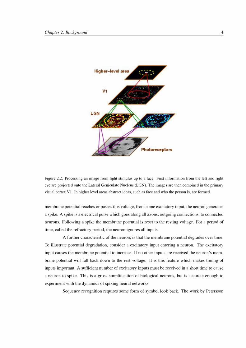
together to identify every possible orientation within a receptive field (RF). This further abstraction
allows stimulus to be aggregated into higher level concepts. In the visual cortex this is combining
information from photons of light, into gradients within a RF then contours and eventually objects,
as illustrated in Figure 2.2 [20].
Minicolumns are collections of approximately 100 neurons which work together to iden-
tify gradient orientations within the RF. The cumulative activity of all neurons produce a single
“result” for the entire group. Pulvermuller [26] postulates that individual neurons are too noisy
and unreliable computational devices so it is advantageous to use sets of neurons together. This
is similar to the strategy used in computing where three CPU’s are used together in computation.
Each CPU performs the same calculation and the final solution is that given by two of the three
CPU’s. Pulvermuller also suggests that if the signal-to-noise ratio of individual neurons is too high,
averaging the activity over a group of neurons, with similar functional characteristics, improves this
ratio. Minicolumns combine the activity of all excitatory neurons within to reduce the noise from
each neuron.
The neurons used in this thesis are based on the integrate and fire model. In this model
a neuron consists of a membrane potential. The membrane potential is equivalent to the internal
voltage of a neuron relative to the extra-cellular space. With no activity the membrane potential
remains at a fixed rest voltage. Input to the neuron is in the form of electrical impulses. The
voltage of inputs can be positive or negative. Positive inputs cause the membrane potential to rise,
this process is called excitation. Negative inputs cause the membrane potential to fall, this process
is called inhibition. A activation threshold is a specific membrane potential voltage. When the
Chapter 2: Background 4
Figure 2.2: Processing an image from light stimulus up to a face. First information from the left and right
eye are projected onto the Lateral Geniculate Nucleus (LGN). The images are then combined in the primary
visual cortex V1. In higher level areas abstract ideas, such as face and who the person is, are formed.
membrane potential reaches or passes this voltage, from some excitatory input, the neuron generates
a spike. A spike is a electrical pulse which goes along all axons, outgoing connections, to connected
neurons. Following a spike the membrane potential is reset to the resting voltage. For a period of
time, called the refractory period, the neuron ignores all inputs.
A further characteristic of the neuron, is that the membrane potential degrades over time.
To illustrate potential degradation, consider a excitatory input entering a neuron. The excitatory
input causes the membrane potential to increase. If no other inputs are received the neuron’s mem-
brane potential will fall back down to the rest voltage. It is this feature which makes timing of
inputs important. A sufficient number of excitatory inputs must be received in a short time to cause
a neuron to spike. This is a gross simplification of biological neurons, but is accurate enough to
experiment with the dynamics of spiking neural networks.
Sequence recognition requires some form of symbol look back. The work by Petersson

Chapter 2: Background 5
et al. [23] found that a 3 symbol look back is required to predict the next symbol from a string
generated by the Reber grammar in Figure 2.1. Macoveanu et al. [17] were able to retain two
concepts in a spiking network. Their model focused on recurrent connectivity, a similar concept is
used in the model in this thesis. Tegner et al. [30] discuss the effect of strongly recurrent networks
on working memory. They postulate that neurons with recurrent connections stimulate each other
to retain a memory. This model is very similar to early computer memory where a single bit was
stored by continuously refreshing a circuit, such as in delay line memory [8].
The minicolumn model developed in this thesis uses the combined activity of all of the ex-
citatory neurons within a given minicolumn to represent a recent input symbol. Dayan [7] suggests
a blackboard-like concept of memory, operating similar to how interpreted languages are executed
on a computer. The currently relevant information is stored on the blackboard and next action is
determined by comparing all actions to the stored information. The model, in this thesis, is designed
to retain activity resulting from presentation of a symbol for the duration of the two subsequent sym-
bols, using active storage as defined by Zipser et al. [34]. This produces a two symbol look-back
within the minicolumn model. The third symbol of look back, as required by Petersson et al. [23],
is achieved through activation of sub-regions of neurons within a network of minicoulmn models.
The activation of these regions indicates that a specific sub-sequence has been observed by the net-
work. Maass et al. [16] and Sandbert et al. [29] use a similar concept of fading memory as a factor
in neuron models. Fading memory means that the influence of any specific segment of the input
stream on later parts of the output stream becomes negligible when the length of the intervening
time interval is sufficiently large [16].
Chapter 3
Model
Using biologically inspired spiking neurons, a network is designed to recognize strings
belonging to the Reber grammar. Extending on work by Petersson [24] using predictive networks
based on the SRN architecture. The project is divided into an input layer and a recognition layer.
The input layer converts ASCII symbols into spiking activity. The recognition layer retains the rules
of the grammar and match the input activity to the rules. The Neural Simulation Tool (NEST) [12]
is used for all modeling and simulation described in this thesis. It provides neuron models and a
framework for simulating large networks. The technical details of how the network is implemented
are covered in Section 4.
3.1 Input layer
The strategy for translating character strings into spiking activity was inspired by sensory
input transduction in the brain. In the auditory system, sound is separated into frequencies in the ear.
Different frequency ranges stimulate separate regions of the auditory cortex [2]. A similar strategy
is used in the visual cortex. Spatial locality of light entering the eye is preserved in the V1 layer
of the visual cortex. The 6 symbols in Reber strings {#,M,T,R,X,V} are treated as separate inputs.
Each symbol causes excitatory activity from a different input node. The input string is presented
one symbol at a time and only the input node of the current symbol is active, which thus corresponds
to lexical detector/retriever in the human brain [14].
These input nodes are in turn connected to minicolumns are sensitive to and “listen”
for specific input patterns and begin spiking once an input is present. This is a simplification of
work by Nima et al. [19] and Mercado et al. [18] where sound waves are converted to spiking
6
Chapter 3: Model 7
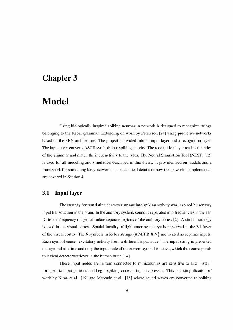
Figure 3.1: The input layer receiving the string “#MTVT#”. When the symbol # is presented the correspond-
ing DC generator, indicated by #, is activated by setting its output rate. This causes the connected minicolumn
to become active and inject activity the rest of the network
activity. Nima et al. [19] represent phonemes based on best rate, best scale, and best frequency;
this representation gives a unique spatial position of each phoneme based on the three dimensions.
The work by Mercado et al. [18] uses a chirplet transform to which . In the simulation, input is
considered a representation of sound, it could also be considered visual or sensory input without
loss of generality. Wang’s paper [33] discusses the concept of RFs in an auditory context.
The input layer is implemented as 6 direct current (DC) generators in NEST. Each is
mapped to a specific input symbol {#,M,X,T,V,R}. When a symbol is presented to the network
the corresponding DC generator is set to a positive amplitude. This can be thought of as the neu-
rons directly excited by external stimuli in real (“wet”; neurophysiological) experiments. Only one
generator is active at a given point in time and all other generators have their amplitude set to zero.
DC generators are in turn connected to input nodes in the recognition layer. Figure 3.1
shows the input layer being presented the first character from the string #MTVT#. The DC generator
representing # is activated, all other generators are silent. The resulting current excites the connected
minicolumn model. Activity will then be propagated to all nodes connected to this minicolumn
model.
3.2 Recognition layer
Artificial Grammar (AG) processing is performed in the recognition layer. The objective
of this layer is to classify strings as belonging to the Reber grammar, or not. The recognition layer
Chapter 3: Model 8
is a network of minicolumns designed to capture the rules of the Reber grammar.
Firstly, a biologically inspired minicolumn of leaky integrate and fire neurons is designed,
described in Section 3.2.1.
The recognition layer is designed to accept sequences generated by the Reber grammar
defined in Figure 2.1. Two strategies were investigated, and two networks designed. One is a com-
plete network with nodes for all bigrams and trigrams in the grammar, shown in Section 3.2.2. The
other attempts to minimize the number of nodes in the network needed to track a string’s position in
the grammar FSM corresponding to the grammar, shown in Section 3.2.3. Both networks, connect
minicolumns in a tree structure designed to recognize subparts of strings. The goal is that activity
in nodes located in lower levels in the tree indicate the presence of substrings in the input strings
of increasing length. In both networks the first level of the tree is connected to the input layer, as
shown in Figure 3.1.
3.2.1 Minicolumn model
Biologically inspired minicolumn models are the main processing units of the network.
Each minicolumn is designed with 100 integrate and fire neurons, 80% excitatory and 20% in-
hibitory. These proportions are based on neurophysiological data [6, 4]. Panzeri et al. use equal
numbers of excitatory and inhibitory neurons in sub-regions of their visual cortex model [22]. This
thesis uses the biologically based numbers to maintian biological integrity in the minicolum model.
Biologically inspired integrate and fire neuron models are used, so that the simulation can be com-
pared to neurophysiological investigation in the future, for example functional magnetic resonance
imaging (FMRI) experiments.
Minicolumns with 10 and 50 neurons were experimented with but were found to produce
insufficient recurrent activity. Connection densities and weights did not scale down to these smaller
models. Macoveanu et al. [17] use networks consisting of 256 excitory and 64 inhibitory neurons
to retain items on the order of seconds.
The models studied in this thesis use local connections within the minicolumn model to
create recurrent activity to represent the presence of input. The first goal of this research is to achieve
degrading persistent spiking within the minicolumn model. In other words, following presentation
of input, the minicolumn should continue spiking from internal recurrent activity of excitatory neu-
rons for a period of two symbol presentations, specified to be 1000 ms in this model (each symbol
is presented for 500ms). At that time, local inhibition overcomes the excitatory activity and the
Chapter 3: Model 9
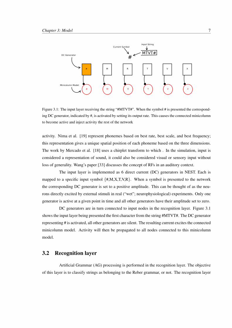
Figure 3.2: A simplified model of connections within the minicolumn. Numbers indicate base delay, in
ms, along the connection. These values are later offset by a random amount to simulate lateral position of
neurons and indirect axon paths. Filled circles represent excitatory connections, empty circles inhibitory.
Each connection type is shown from only one neuron.
neurons return to their unexcited activity rates. This effectively provides a 2 symbol look-back slid-
ing window memory mechanism, since each symbol is presented for 500ms. This time period was
chosen to be biologically plausible based on behvioral and neurophysological experiments with hu-
mans. For example, Alain et al. [2] present auditory stimuli to human subject for 500ms with 5ms
rise/fall time and Forkstam et al. [11] presented sequences of symbols from the Reber grammar for
500ms each with a 300ms inter-symbol-inveral. In this thesis, working memory is conceptualized
as a type of online memory attributed to spiking activity. The retention times used in this thesis is
consistent with other research which retain information for multiple seconds [3, 30].
Leaky integrate and fire neurons are used for all neurons in the model. This approximates
the behaviour of biological neurons using a mathematical model of neuron activity as defined by
Rotter and Diesmann[28]. This is a standard approximation which is computationally efficient and
allows simulation of large networks [15].

Chapter 3: Model 10
The leaky integrate and fire neurons have a rest/reset membrane potential of -75mV and
a firing threshold at -55mV. An absolute refractory period (T Ref) of 5ms is used. This is necessary
to achieve activity rates at a biologically plausible level (∼ 35Hz). Shorter T ref, for example 1 ms,
results in spiking frequencies of 100 to 200 Hz, non-biologically plausible rates.
Each excitatory neuron is connected to ∼ 40% of other excitatory neurons, and ∼ 25% of
inhibitory neurons. Each inhibitory neuron is connected to ∼ 15% of excitory neurons. Figure 3.2
shows a simplified view of local minicolumn connections. Each type of connection (excitatory-
excitatory, excitatory-inhibitiory, inhibitory-excitatory) from one neuron are shown. There are no
inhibitory to inhibitory connections which is consistant with neurobiological networks [4]. When
connections are made, each neuron is connected to a set of neurons randomly selected from the
available population within the minicolumn.
For example, given an excitatory neuron x from the collection of all excitatory neurons,
Excite, then the set of excitatory neurons x will connect to is obtained by randomly selecting 40% of
remaining excitatory neurons. For excitatory-inhibitory connections, 25% of inhibitory neurons are
selected. The randomized connectivity procedure ensures that the connections in each minicolumn
model are not identical.
Spatial locality is built into the model. Neurons are laid out as in Figure 3.2 with the
inhibitory neurons placed in the middle of the excitatory neurons. For two neurons, x and y, the
distance between them, dist, is calculated with the neurons position in an array. Compte et al. [5]
use a circular neuron layout where angles between neurons introduce variation in the connection
delay.
For two excitatory neurons, x and y, in the array, Excite the distance is calculated as in
Equation 3.1. For an excitatory neuron, x, and an inhibitory, i, in the array, Inhib the distance is
calculated as in Equation 3.2. INHIB ORIGIN is the position on the excitatory array where the first
inhibitory neuron lies. For example, in Figure 3.2 INHIB ORIGIN = 3.
dist = abs(Excite.index(y)−Excite.index(x)) (3.1)
dist = abs(Excite.index(x)− (INHIB ORIGIN +Excite.index(i))) (3.2)
A random delay, offset, in the range of±2.5ms is applied to each connection to simulate
lateral location of the neuron and non-direct axon paths, offset is calculated by Equation 3.3. Total
connection delay, del, is calculated by Equation 3.4. A minimum of 1ms delay is required by NEST.
Chapter 3: Model 11
If del < 1ms then del is set to 1ms.
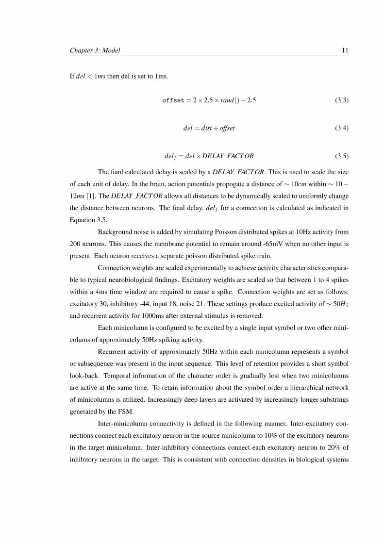
offset = 2×2.5× rand()−2.5 (3.3)
del = dist +offset (3.4)
del f = del×DELAY FACTOR (3.5)
The fianl calculated delay is scaled by a DELAY FACTOR. This is used to scale the size
of each unit of delay. In the brain, action potentials propogate a distance of ∼ 10cm within ∼ 10−12ms [1]. The DELAY FACTOR allows all distances to be dynamically scaled to uniformly change
the distance between neurons. The final delay, del f for a connection is calculated as indicated in
Equation 3.5.
Background noise is added by simulating Poisson distributed spikes at 10Hz activity from
200 neurons. This causes the membrane potential to remain around -65mV when no other input is
present. Each neuron receives a separate poisson distributed spike train.
Connection weights are scaled experimentally to achieve activity characteristics compara-
ble to typical neurobiological findings. Excitatory weights are scaled so that between 1 to 4 spikes
within a 4ms time window are required to cause a spike. Connection weights are set as follows:
excitatory 30, inhibitory -44, input 18, noise 21. These settings produce excited activity of ∼ 50Hz
and recurrent activity for 1000ms after external stimulus is removed.
Each minicolumn is configured to be excited by a single input symbol or two other mini-
colums of approximately 50Hz spiking activity.
Recurrent activity of approximately 50Hz within each minicolumn represents a symbol
or subsequence was present in the input sequence. This level of retention provides a short symbol
look-back. Temporal information of the character order is gradually lost when two minicolumns
are active at the same time. To retain information about the symbol order a hierarchical network
of minicolumns is utilized. Increasingly deep layers are activated by increasingly longer substrings
generated by the FSM.
Inter-minicolumn connectivity is defined in the following manner. Inter-excitatory con-
nections connect each excitatory neuron in the source minicolumn to 10% of the excitatory neurons
in the target minicolumn. Inter-inhibitory connections connect each excitatory neuron to 20% of
inhibitory neurons in the target. This is consistent with connection densities in biological systems
Chapter 3: Model 12
[6]. A larger minimum delay of 3ms is applied to all long-distance interconnections between mini-
columns to represent the larger distances between minicolumns.
Petersson points out that from a neurophysiological perspective it is reasonable that the
brain has finite memory resources [23]. A result of this is the length of substrings which can be
represented in the network is limited to three symbols. The Hierarchical Temporal Memory (HTM)
srategy introduced by Hawkins et al. [13] uses layers of neruons to model the cortex. The model
used in this thesis uses networks to represent the hierarchical connectivity distribution observed in
the primate brain [9], in which concepts are learned and stored and combinations of these concepts
are used to identify more abstract entities.
3.2.2 Complete Network
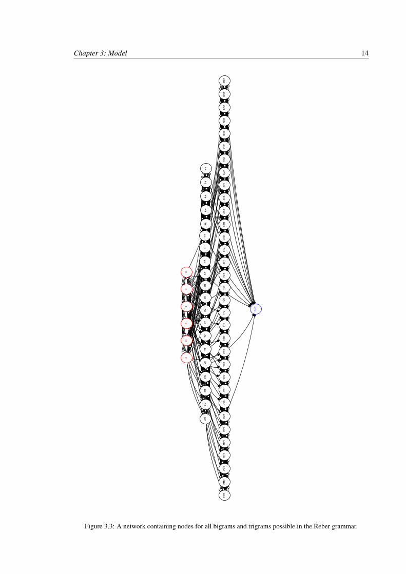
Petersson determined that a machine which can represent the set of all bigrams and tri-
grams, TG, can recognize a Reber Grammar. The complete network, see Figure 3.3, implements this
strategy. This network contains 60 nodes. Activity in a node indicates that the associated substring
has appeared in the input. Nodes are arranged in 4 layers. The first layer contains 6 nodes actived
by individual symbols and is connected to the input layer, as shown in Section 3.1. The second
layer contains 20 nodes which activate to all bigrams in the grammar. The third layer contains 33
nodes which activate to trigrams in the grammar. At the bottom of the network is the output layer
consisting of a 1 OUT node.
All nodes will be refered to by the substring their activation represents, for example node
# is the node in the first layer which is activated when symbol # is presented to the network. The
layer a node belongs to is equal to the number of symbols in it’s name.
Nodes in the second layer recieve input only from nodes in the first layer, for example the
node #M recieves input from node # and node M. Each node receives input from the nodes which
are activated by the symbols in the bigram they represent.
Each node in the third layer receive input from one node in the second layer and one on
the first layer. For example the node #MV receives input from node #M and node V. Node # and M
are not connected to #MV because at the time when symbol V is presented to the activity in node #
is irrelevant to the trigram #MV. In the case where the input string is gramatical then node # should
be silent when V is presented, two symbols later. In the case when the string is not gramatical and
perhaps # is presented again then the trigram #MV is isolated from this activity and will not become
active.

Chapter 3: Model 13
The OUT node is stimulated by all nodes which can end a grammar string, for example
node MV#. Each node in the layers 2 to 4 require at least two connected nodes to be active to
become active.
At each level only one node is fully active at a given time. Fully active is defined as
spiking activity above 50Hz. To facilitate this each level of the network is completely connected
with inhibitory connections. A competition exists between nodes in each layer. The node currently
or most recently receiving input should have the highest activity in the layer. That node will provide
the most excitement to the inhibitory neurons all other minicolumns in the same level. This keeps
the activity under control and limits the affect of past activity from causing the network to recognize
a string. Only the most current substring should be represented in the network.
The complete network contains 1466 inter-inhibitory links and 121 inter-excitatory links.
These are links which result in 80×8 = 640 connections for each inter-excitatory link and 80×4 =
320 connections for each inter-inhibitory link. This results in 546560 inter-minicolumn connections,
as calculated in Equation 3.6.
(1466×320)+(121×640) = 546560 (3.6)
In the complete and the minimized network, recognition is defined by the OUT node
spiking at over 35Hz during the 500ms after the end of string # symbol is presented to the network.
Activity is calculated in this way because it takes approximately 250ms for activity to propogate
from one layer to the next. For this reason the OUT node activates from the end of the string almost
750ms after the # symbol is presented to the network. The performance of this network is presented
in Section 5.
3.2.3 Minimized network
The objective of the minimized network was to reduce the number of nodes needed to
recognize substrings by reusing lower level nodes, shown in Figure 3.4. Only 20 nodes are used
in this network as opposed to 60 nodes in the complete network. The major difference to the
complete network is a much lower number of trigram nodes. Many of these nodes have no outgoing
connections in the complete network and do not contribute to string recognition.
Nodes are selected by traversing the FSM and adding nodes which uniquely identify
states. For example MV, VT, VX indicate the edge into and out of a state of the FSM. It was
found that most trigrams were not necessary represent with this scheme. The trigrams which are
Chapter 3: Model 14
Figure 3.3: A network containing nodes for all bigrams and trigrams possible in the Reber grammar.
Chapter 3: Model 15
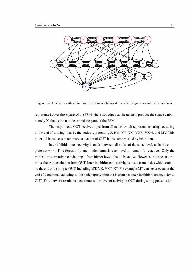
Figure 3.4: A network with a minimized set of minicolumns still able to recognize strings in the grammar.
represented cover those parts of the FSM where two edges can be taken to produce the same symbol,
namely X, that is the non-deterministic parts of the FSM.
The output node OUT receives input from all nodes which represent substrings occuring
at the end of a string, that is, the nodes representing #, RM, VT, XM, VXR, VXM, and MV. This
potential introduces much more activation of OUT but is compensated by inhibition.
Inter-inhibition connectivity is made between all nodes of the same level, as in the com-
plete network. This forces only one minicolumn, in each level to remain fully active. Only the
minicolum currently receiving input from higher levels should be active. However, this does not re-
move the extra excitation from OUT. Inter-inhibition connectivity is made from nodes which cannot
be the end of a string to OUT, including MT, VX, VXT, XT. For example MT can never occur at the
end of a grammatical string so the node representing the bigram has inter-inhibition connectivity to
OUT. This network results in a continuous low level of activity in OUT during string presentation.
Chapter 4
Modeling Framework
To enable rapid prototyping of network parameters and layouts a framework was devel-
oped. This framework provides facilities to import parameter data from an OpenDocument spread-
sheet (ods) file. Network layouts are drawn in the diagram program Dia. The framework is able
to extract the network details from the .dia file and construct the network for the simulation. The
network, defined in the diagram, is built using the minicolumn model, described in Section 3.2.1,
and NEST connections. Dia scripts were created to aid with network creation, they will be discribed
in Section 4.2.
4.1 Parameters
The heart of the simulation is the parameters which define how the network will behave.
The nieve method of managing parameters is to define all values directly in the code of the project.
This is a very bad way to set parameter values, since they will be changed often. When an change
is to be made every instance of that parameter must be changed. A better approach is to define
all parameters as variables in one place in the code. With this method changing a parameter value
envolves changing the variable value once.
The code needed to build the network and run a simulation is contained in nine python
script files. Each of these contain parameters which have an affect on the simulation. Having
the parameters in multiple places pose new challanges, changing these values requires opening the
required python script files and modifying the parameters. In this project it is required to sharing
the parameters with different people to decide what their values should be. Sharing the parameters
requires packaging and sending all python files. Maintaining multiple versions of parameters require
16

Chapter 4: Modeling Framework 17
A B1 Parameter Name Parameter Value2 . .3 . .
Table 4.1: Template of parameter spreadsheet
multiple versions of the python files where the only difference may be one line. This is an inneficient
and redundant way to manage parameters.
A list of aspects of the simulation controlled by parameters follows:
• Minicolumn size (number of excitory and inhibitory neurons)
• inter connection density
• intra conneciton density
• connection weight
• connection delay
• neuron parameters
• noise rate
• graph creation
• save directories
To remove the dependancy to the python files, all parameters are placed in a spreadsheet.
This reduces the time to change parameters. Another advantage is to be able to see all parameters
at once. Making it easier to understand the impact each parameter has on the whole simulation. A
standard file format, ods, was the natural choice for sharing parameter configurations. Given the
openness of the format and the fact information is stored in eXtensible Markup Language (XML) it
was possible to parse the files in python. The parameters within the simulation can then be set to the
values specified in the spreadsheet. The parameter file must have the format described in Table 4.1.
Only values in columns A and B are processed, everything else is ingored. Other columns can be
used for descriptions of parameters or scratch work.
Chapter 4: Modeling Framework 18
The file is parsed into a python dictionary indexed by parameter name with parameter
value as the associated values. All variables declared in the simulation are collected and considered
one by one. If a parameter name in the loaded dicitonary matches a variable name, the variable is
set to the associated parameter value. Any information not matching an existing variable is ignored.
This allows parameters to be organized in the ods with headings or spaces to improve readability.
All headings and spaces will be ignored, unless a parameter name in the code exactly matches the
heading text. This solution has the benifit that new parameters can be added to the parameter file
without modifying any code. If new modules are to be used in the simulation, with variables which
will be specified in the parameter file, the only change required is to add the module name to a list
of all modules.
Abstracting the parameters into a spreadsheet allows changes to be quickly made and
applied to the simulation. Multiple versions of the spreadsheet can be used to represent different
network configurations. Collaboration now requires exchanging one spreadsheet file instead of
many code files. A similar method of abstraction is used to define network layout, this method is
described in Section 4.2.
4.2 Network Building
Constructing the network layout programmatically introduce many of the same problems
faces with managing network parameters. Making changes to network layour requires making
changes to the code. Changing the connection of one minicolumn to another requires one code
change, adding or removing a node can require many more changes depending on how many nodes
are connected to it and how many nodes it is connected to. To communicate the network topology to
others it is necessary to draw a diagram of the network. The diagram allows the network to be easily
visualized and analyzed but is seperate from the representation of then network in code. Changes
to the network require modifications in two places; to the code and the diagram. If changes are not
properly replicated the code and diagram become inconsistent and irrelivant. Use of a diagraming
program which saves diagrams in a parsible format can eliminate this extra work.
The diagram drawing program Dia was used in this project. This program provides an
extensive library of shapes and connections as well as a XML based save file. Python has also
been integrated with Dia, allowing scripts to be written which can manipulate the diagram. The
network layout can exist in one form which is used both to visualize the network and to run the
simulation. Changes to the network are made in one place. An added bonus is identifying missing

Chapter 4: Modeling Framework 19
Figure 4.1: The Dia types needed to build networks for the framework
or extra connections requires only a visual inspection of the network. Multiple network layouts can
be maintained in parallel and run through the framework without requiring code changes.
To facilitate reading of .dia files a few guidlines must be followed when creating the net-
work. The following objects must be used: Dia ’Standard - Ellipse’ objects represent a minicolumn.
’Standard - Text’ objects linked to the ellipses specify the name of the minicolumn. The colour of
the text indicated if the minicolumn should receive input directly, or if it will be an output. Input
minicolumns are indicated with red text. The name of the label must be one of the possible symbols
of the Reber grammar {#, M, V, X, R, T}. Output minicolumns are indicated with blue text. The
name of the label must be ’OUT’. All other minicolumns have black text. Connections are made
with ’Standard - Arc’ objects. These are directed connections with the end arrow indicating an ex-
citatory connection or inhibitory connection. Excitatory connections are represented with a closed
circle (arrow number 8) end arrow. These will result in the excitatory neurons of the start minicol-
umn being connected to the excitatory neurons of the target minicolumn. Inhibitory connections
are represented with a open cirlce (arrow number 9). These will result in the excitatory neurons of
the start minicolumn being connected to the inhibitory neurons of the target minicolumn. Labels
and connections must be anchored to the nodes. The basic network components are illustrated in
Figure 4.1.

Chapter 4: Modeling Framework 20
Output Descriptionnodes the Dia id of all nodes in the net-
worknodelabels [name,id] tuples for all nodesexcite connections [start id, end id] tuples of all ex-
citory connectionsinhib connections [start id, end id] tuples of all in-
hibitory connectionsinputnodes [input symbol, id] tuples of all
input nodesoutputnode [node label, id] tuple of output
note(s)
Table 4.2: Results from parsing a .dia file representing a network layout
Parsing the network layout is carried out with a ContentHandler object which is provided
to the XML parser. Each object is processed indipendantly and stored in Lists. Any objects not
following the above guidelines are ignored. The end results are described in Table 4.2
Two python scripts were created to aid in the contstruction of networks with NEST. The
first is designed to help with creating inhibitory connections between nodes in a layer. The script
completely connects all selected nodes. For n nodes, n(n−1) connections are made in O(n2) time.
The second script connects nodes based on their labels. Labels are assumed to be concate-
nations of names of nodes which they should receive input from. For example, the node named #M
will receive input from the # node and the M node. This script iterates through all nodes creating at
most 2 connections for each node in O(n) time.
Chapter 5
Results
Simulations were performed with the complete and minimized network to determine the
feasibility of their design at AG recognition. Both networks were given the same grammatical, non-
grammatical, and random sequences, shown in Appendix C. The grammatical and non-grammatical
sequences both contain 17 strings. The random sequence also contains 17 strings. The same network
parameters were used in all simulations to control for all variable except network layout, shown in
Appendix B.
Non-grammatical strings were manually created by altering individual symbols in the
grammatical string. This is consistent with how strings are constructed for physiological tests [10,
11, 25, 32]. Random strings such as, MVVRVV, are generated by selecting one symbol from the
alphabet, {#, M, V, T, R, X}, where each symbol has equal probability of being selected for each
position. Strings generated this way are generally non-grammatical, some empty strings are also
produced, for example ## which does not contain a symbols. These are removed in post processing
since double # will cause the output node to activate. Grammatical strings have at least 2 symbols
between # symbols.
Random non-grammatical strings are easily identified as non-grammatical by the network
when no valid substrings exist. A string such as, #MTRT#, is more difficult to identify as non-
grammatical since only one symbol is incorrect. The network can falsely recognize these strings if
the last substrings are grammatical. The networks being able to recognize these types of strings as
non-grammatical provide very good support for their use in futher computational studies.
Network activity was analyzed through spike train analysis. The spike activity of all
neurons in a given minicolumn is collected throughout the simulation. Histograms are then plotted
to analyze spiking rates. The input sequence used is set as the x-axis of the histogram plot so that
21

Chapter 5: Results 22
activity can be correlated to characters being presented. Recognition is defined as the output node
having an average activity of 35Hz for the 500 ms following the end of string symbol #.
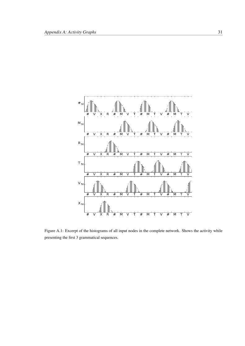
The activity from the first 3 grammatical strings are presented in Figures A.1, A, A.3, and
A.4. The current input character is indicated along the x axis of all graphs. The histogram shows
average activity of all excitatory nuerons in the minicolumn model over time. The DC generator
assigned to that symbol is producing spike trains which are being directed at the corresponding node
in the input layer for 500ms. After 500ms a new symbol is presented. The DC generator associated
to that symbol is activated and all others are silenced as described in Section 3.1. The activity in
Figure A.1 shows that input nodes are active within 250ms of input being presented and remain
active for 500ms after input is removed. This activity pattern allows activity of two nodes of the
input layer to excite a node in the second layer.
In the example the first two symbols are # and V. At time 750ms, halfway through pre-
sentation of V, both # and V have activity above 50Hz. This activity is able to excite node #V, in
Figure A, to become active. The activity in #V then continues until time 1750 when R is being
presented. At this time both # and V are themselves silent. Note also that node V# is active at
almost the same time, this is an undesired affect but a result of # being active toward the end of V’s
presentation time. As the activity propogates to layer three node #VX is activated by #V and X from
layer one. This continues for the R and the end of string #. At that point the nodes R#, and XR# are
active and cause the OUT node to activate past the recognition level. At that point the network has
recognized the string.
The other input strings are presented in this way, with similar results.
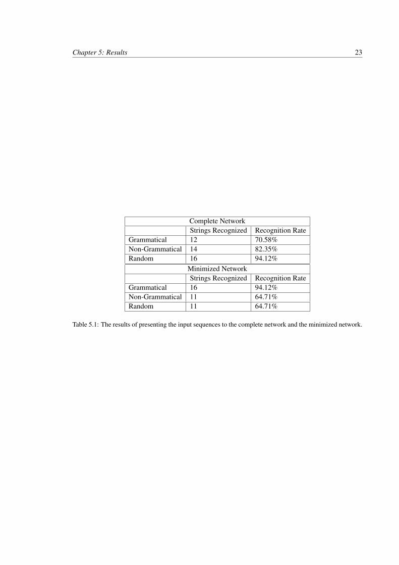
The results of the simulation for both networks are shown in Table 5.1. The recogni-
tion rates alone show promise but leave room for improvement. For the complete network no
discrimination was observed: 12 of 17 grammatical strings were correctly recognized, 14 of 17
non-grammatical and 16 of 17 random strings were incorrectly recognized. The minimized network
has slightly better performance: 16 of 17 grammatical strings are correctly recognized, 11 of 17
non-grammatical strings and 11 of 17 random strings are incorrectly recognized. This poor perfor-
mance over the input sequences is the result of using the same input parameters for both networks.
The networks are so different in topology that it is biologically feasible that the parameters, specif-
ically connection weights, should be different as well. Strategies to improve recognition rates are
discussed in Section 6.
Chapter 5: Results 23
Complete NetworkStrings Recognized Recognition Rate
Grammatical 12 70.58%Non-Grammatical 14 82.35%Random 16 94.12%
Minimized NetworkStrings Recognized Recognition Rate
Grammatical 16 94.12%Non-Grammatical 11 64.71%Random 11 64.71%
Table 5.1: The results of presenting the input sequences to the complete network and the minimized network.
Chapter 6
Discussion
It has been demonstrated that AG recognition is feasible in spiking neural networks. It is
also evident that this thesis only touches upon the tip of the iceberg of what is possible. The original
inspiration of this thesis was to produce models closely based on specific physiological theories
of the neocortical structure of brains. The ability to meet these goals was limited mainly by two
factors; firstly, the technical hurdles faced were vast; secondly, the lack of a unified theory of neural
structure based on neuroimaging and neurophysiological experiments could not be found.
The poor performance of the networks is a result of the use of a single set of parameters
for both networks. With networks as different as the complete network and minimized network it is
neccessary for the dynamics to be different. Parameters were optimized to find a balance between
the two networks. This results in suboptimal performance in both networks. A seperate set of
parameters should be used for both networks. The performance of the minimized network can be
greatly improved. Past results from this project focusing on the minimized network did have much
better recognition rates.
Focus should be placed on the network activity patterns, shown in Appendix A. The
graphs demonstrate that the networks are able to represent substrings of grammatical strings. That
the network can be fooled by strings which contain grammatical substrings is realistic to human
performance. The goal of this project was not to construct networks which perfectly recognize
strings from the grammar. Further analysis can compare the networks performance compare to
human performance in a similar recognition task.
Future directions the work presented in this thesis may take are to explore flexibility and
learning in the network. In this thesis the network is created with an inherent preference for the
Reber grammar. A natural next step would be to begin with a more generic form of the network
24

Chapter 6: Discussion 25
with a number of nodes perhaps between the minimized network and the complete network. The
nodes should be completely connected to one another with adapting synapses. Train the network
by feeding input to specific input nodes. Then present many grammatical strings. Through synaptic
adaptation and pruning (if the synapse weight becomes negligibly small) see if a functional network
emerges. Test the network by presenting grammatical strings not in the training set as well present
non-grammatical strings and see if the network performs at a rate similar to human performance.
Another strategy would be to use genetic programming to evaluate an optimal network layout and
parameter settings for the network.
More tools can be written to improve usability of the modeling framework. Improvements
in the framework will facilitate collaboration between physiological researchers and modeling re-
searchers. The framework can be used as a tool to test network layouts from imaging studies.
Spiking models can be used with physiological studies to compare human performance
to the simulation. By continuing work on the model and applying new theories arrising from hu-
man performance and imaging data perhaps a better understanding of the missing dimension can
be found. This missing dimension, is ability to observe brain function at a very high resolution.
The ability to know read the layout of the coretex and observe it’s activity. Imaging technologies
available today (Magnetic Resonance Imaging (MRI), Positron Emission Tomography (PET), Elec-
troencephalography (EEG)) view the brain at a very low resolution, relative to individual neurons.
Only activity in groups of neurons can be seen. Images produced contain a lot of noise and statis-
tical methods are used to extract brain activity. Interconnections between individual neruons can
only be guessed. How neurons are connected and where excitation and inhibition appear cannot be
seen. A closer view of neurons is only possible with very evasive techniques. For exable, inserting
electrodes in the brain to record activity in small groups of neurons. These techniques are limited
by how many electrodes can be inserted before brain function is impared. Beyond this individual
neurons can be tested in wet experiments. Isolated from the rest of the network, how the extracted
neruons interact in the system cannot be determined. Slices of cortex can be analized for structure
but neruons are not two dimensional nor are their connections, such slices give only a partial image
of the network of the brain. The challange in understanding the brain is combining these techniques.
Models of the cortex as presented in this thesis are an important step in combining what is known
about the brain. These techniques will form a symbiotic relationship in which advancements in
modeling will improve physiological studies and vice versa.

Acknowledgments
I am indebted to my supervisor, Baran Curuklu, Malardalen Hogskola, for setting me on
this path of neural modeling. He has given me the opportunity to explore the field of cognitive
science, which has intreagued me for many years. I am grateful for his guidance and support (and
all the lattes and muffins). Without his enthusiasm and great ideas this project would not have been
possible. He kept me striving for a biologically realistic minicolumn model.
I would like to thank my other supervisor, Karl Magnus Petersson, FC Donders Centre
for Cognitive Neuroimaging, for setting realistic objectives for this project and sharing your vast
knowledge of grammar processing in physiological and modeling experiments. Without his help it
would have taken years to complete this project.
Many thanks to Julia Udden, Eva Cavaco, and Paul Teichmann who read the very rough
draft of this thesis. Their comments helped focus my scattered thoughts and bring unity to this
thesis.
Thank you Martin Ingvar and everyone in the Stockholm Brain Institute (SBI) MRC lab,
for giving me a place to work on my project. Thank you to all of the researchers especially Mimmi,
Andrew, Jonathan, Karin, Jeremy, Sissela, Deepak, Fiona, Katarina, Jonas, Stina, whos friendship
and support has made this year an amazing experience.
I would like to thank Leif and Nancy for welcoming me into their home and making it
possible to live in Stockholm with CSN. A thousand thanks to my family, without their love and
support I would not be where I am today. A very special thank you to Jessica for putting up with
me when the details would get the better of me and listening when all I could talk about was the
project.
26

Bibliography
[1] F Aboitiz, A B Scheibel, R S Fisher, and E Zaidel. Fiber composition of the human corpus
callosum. Brain Research, 598:143–153, 1992.
[2] Claude Alain, Stephen R. Arnott, and Stephanie Hevenor. ”What” and ”where” in the human
auditory system. PNAS, 98:12301–12306, October 2001.
[3] Alan Baddeley. Working memory: An overview. In Susan J. Pickering, editor, Working
Memory and Education, pages 1 – 31. Academic Press, Burlington, 2006.
[4] D. P. Buxhoeveden and M. F. Casanova. The minicolumn hypothesis in neuroscience. Brain,
125:935–951, May 2002.
[5] A. Compte, N. Brunel, P. S. Goldman-Rakic, and X. J. Wang. Synaptic mechanisms and
network dynamics underlying spatial working memory in a cortical network model. Cerebral
Cortex, 10(9):910–923, September 2000.
[6] Baran Curuklu. A Canonical Model of the Primary Visual Cortex. PhD thesis, Malardalen
University, March 2005.
[7] Peter Dayan. Simple substrates for complex cognition. Frontiers in Neuroscience, 2, Decem-
ber 2008.
[8] J.p. Jr. Eckert. A survey of digital computer memory systems. IEEE Annals of the History of
Computing, 20(4):15–28, 1998.
[9] D. J. Felleman and D. C. Van Essen. Distributed hierarchical processing in the primate cerebral
cortex. Cereb. Cortex, 1:1–47, 1991.
[10] V. Folia, J. Udden, C. Forkstam, M. Ingvar, P. Hagoort, and K. M. Petersson. Implicit learning
and dyslexia. Ann. N. Y. Acad. Sci., 1145:132–150, Dec 2008.
27

Bibliography 28
[11] C. Forkstam, P. Hagoort, G. Fernandez, M. Ingvar, and K. M. Petersson. Neural correlates of
artificial syntactic structure classification. Neuroimage, 32:956–967, Aug 2006.
[12] O. Gewaltig and M. Diesmann. Nest (neural simulation tool). Scholarpedia, 2(4):1430, 2007.
[13] Jef Hawkins. Learn like a human: Why can’t a computer be more like a brain? IEEE Spectrum,
April 2007.
[14] Ray Jackendoff. Foundations of Language: Brain, Meaning, Grammar, Evolution. Oxford
University Press, 2002.
[15] Collin J. Lobb, Zenas Chao, Richard M. Fujimoto, and Steve M. Potter. Parallel event-driven
neural network simulations using the hodgkin-huxley neuron model. In PADS ’05: Proceed-
ings of the 19th Workshop on Principles of Advanced and Distributed Simulation, pages 16–25,
Washington, DC, USA, 2005. IEEE Computer Society.
[16] Wolfgang Maass, Prashant Joshi, and Eduardo D Sontag. Computational aspects of feedback
in neural circuits. PLoS Comput Biol, 3(1):e165, Jan 2007.
[17] J. Macoveanu, T. Klingberg, and J. Tegner. A biophysical model of multiple-item working
memory: a computational and neuroimaging study. Neuroscience, 141:1611 – 1618, 2006.
[18] Eduardo III Mercado, Catherine Myers, and Mark A. Gluck. Modeling auditory cortical pro-
cessing as an adaptive chirplet transform. Neurocomputing, 32-33:913–919, 2000.
[19] Nima Mesgarani, Stephen David, and Shihab Shamma. Representation of phonemes in pri-
mary auditory cortex: How the brain analyzes speech. ICASSP, 2007.
[20] Risto Miikkulainen, James A. Bednar, Yoonsuck Choe, and Joseph Sirosh. Computational
Maps in the Visual Cortex. Springer, Berlin, 2005.
[21] V B Mountcastle. The columnar organization of the neocortex. Brain, (120):701–722, 1997.
[22] S. Panzeri, F. Petroni, and E. Bracci. Exploring structure-function relationships in neocortical
networks by means of neuromodelling techniques. Med Eng Phys, 26:699–710, Nov 2004.
[23] Karl Magnus Petersson. On the relevance of the neurobiological analogue of the finite-state
architecture. Neurocomputing, 65-66:825–832, 2005.

Bibliography 29
[24] Karl Magnus Petersson, Peter Grenholm, and Christian Forkstam. Artificial grammar learning
and neural networks. Proceeding of the Cognitive Science Society 2005, 2005.
[25] K.M. Petersson, C. Forkstam, and M. Ingvar. Artificial syntatctic violations activates Broca’s
region. Cognitive Science, 28:383–407, 2004.
[26] Friedemann Pulvermuller. A brain perspective on language mechanisms:from discrete neu-
ronal ensembles to serial order. Progress in Neurobiology, 67:85–111, 2002.
[27] A S Reber. Implicit learning of artificial grammars. Journal of Verbal Learning and Verbal
Behavior, 6:855–863, 1967.
[28] S. Rotter and M. Diesmann. Exact digital simulation of time-invariant linear systems with
applications to neuronal modeling. Biological Cybernetics, 81:381–402, Nov 1999.
[29] A. Sandberg, A. Lansner, and K. M. Petersson. Selective enhancement of recall through plas-
ticity modulation in an autoassociative memory. Neurocomputing, 38-40:867–873, 2001.
[30] J. Tegner, A. Compte, and X. J. Wang. The dynamical stability of reverberatory neural circuits.
Biological Cybernetics, 87(5-6):471–481, December 2002.
[31] J Udden, S. Araujo, C. Forkstam, M. Ingvar, P. Hagoort, and K.M Petersson. A matter of time:
Implicit acquisition of recursive sequence structures. In Proceedings of the Cognitive Science
Society, 2009.
[32] J. Udden, V. Folia, C. Forkstam, M. Ingvar, G. Fernandez, S. Overeem, G. van Elswijk, P. Ha-
goort, and K. M. Petersson. The inferior frontal cortex in artificial syntax processing: an rTMS
study. Brain Research, 1224:69–78, Aug 2008.
[33] Xiaoqin Wang. Neural coding strategies in auditory cortex. Hearing Research, In Press,
Corrected Proof, 2007.
[34] D. Zipser, B. Kehoe, G. Littlewort, and J. Fuster. A spiking network model of short-term active
memory. Journal of Neuroscience, 13:3406–3420, 1993.
Appendix A
Activity Graphs
30
Appendix A: Activity Graphs 31
Figure A.1: Excerpt of the histograms of all input nodes in the complete network. Shows the activity while
presenting the first 3 grammatical sequences.

Appendix A: Activity Graphs 32
Figure A.2: Excerpt of the histograms of a subset of second layer nodes in the complete network. Shows the
activity while presenting the first 3 grammatical sequences. Observe that activation of the correct nodes does
not guarantee activation of a later node, as with node T#. Node TT is inhibiting T# at this time.

Appendix A: Activity Graphs 33
Figure A.3: Excerpt of the histograms of a subset of third layer nodes in the complete network. Shows the
activity while presenting the first 3 grammatical sequences.

Appendix A: Activity Graphs 34
Figure A.4: Excerpt of the histograms of the output node in the complete network. Shows the activity while
presenting the first 3 grammatical sequences.
Appendix B
Parameters
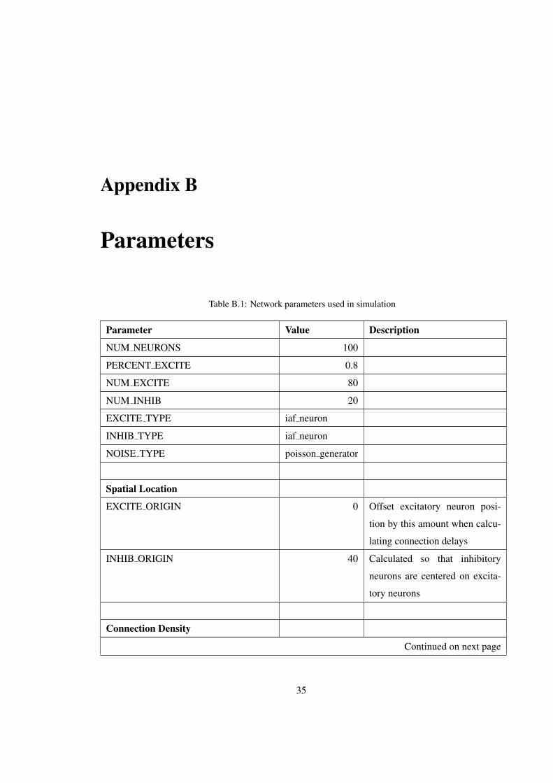
Table B.1: Network parameters used in simulation
Parameter Value Description
NUM NEURONS 100
PERCENT EXCITE 0.8
NUM EXCITE 80
NUM INHIB 20
EXCITE TYPE iaf neuron
INHIB TYPE iaf neuron
NOISE TYPE poisson generator
Spatial Location
EXCITE ORIGIN 0 Offset excitatory neuron posi-
tion by this amount when calcu-
lating connection delays
INHIB ORIGIN 40 Calculated so that inhibitory
neurons are centered on excita-
tory neurons
Connection Density
Continued on next page
35

Appendix B: Parameters 36
Table B.1 – continued from previous page
Parameter Value Description
EXCITE TO EXCITE PERCENTAGE 0.4 Percentage of all other excita-
tory neurons that each excitatory
neuron connects to
EXCITE TO EXCITE CONNECTIONS 32
EXCITE TO INHIB PERCENTAGE 0.25 Percentage of all inhibitory neu-
rons that each excitatory neuron
connects to
EXCITE TO INHIB CONNECTIONS 5
INHIB TO EXCITE PERCENTAGE 0.15 Percentage of excitatory neurons
that each inhibitory neuron con-
nects to
INHIB TO EXCITE CONNECTIONS 12
INHIB TO INHIB PERCENTAGE 0 Percentage of other inhibitory
neurons that each inhibitory neu-
ron connects to
INHIB TO INHIB CONNECITIONS 0
INTER PERCENTAGE 0.1 Percentage of excitatory neurons
in next minicolumn that each ex-
citatory neuron should connect
to
INTER EXCITE CONNECTIONS 8 Number of excitatory neurons in
next minicolumn that each exci-
tatory neurons should connect to
INTER INHIB PERCENTAGE 0.2 Percentage of excitatory neurons
in next minicolumn that each ex-
citatory neuron should connect
to
Continued on next page

Appendix B: Parameters 37
Table B.1 – continued from previous page
Parameter Value Description
INTER INHIB CONNECTIONS 4 Number of inhibitory neurons in
next minicolumn that each exci-
tatory neuron should connect to
Connection Weights
EXCITE WEIGHT 30 Weight of every excitatory con-
nection
INHIB WEIGHT -44 Weight of every inhibitory con-
nection
INPUT WEIGHT 18 Weight of every input connec-
tion
NOISE WEIGHT 21 Weight of every noise connec-
tion
INTER WEIGHT 19 Weight of inter minicolumn con-
nections
INTER INHIB WEIGHT 11 Weight of inter minicolumn in-
hibitory connections
Connection Delays
DELAY FACTOR 1.5 scale each delay unit by this
amount
NOISE DELAY 1 Delay of noise connections in
milliseconds
BASE DELAY 1 Basic Delay of all connections in
milliseconds
INTER BASE 2 Base delay of all inter-
connections
INTER DELAY 1 Base delay for inter minicolumn
connections
Continued on next page
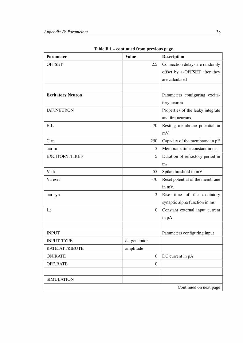
Appendix B: Parameters 38
Table B.1 – continued from previous page
Parameter Value Description
OFFSET 2.5 Connection delays are randomly
offset by +-OFFSET after they
are calculated
Excitatory Neuron Parameters configuring excita-
tory neuron
IAF NEURON Properties of the leaky integrate
and fire neurons
E L -70 Resting membrane potential in
mV
C m 250 Capacity of the membrane in pF
tau m 5 Membrane time constant in ms
EXCITORY T REF 5 Duration of refractory period in
ms
V th -55 Spike threshold in mV
V reset -70 Reset potential of the membrane
in mV.
tau syn 2 Rise time of the excitatory
synaptic alpha function in ms
I e 0 Constant external input current
in pA
INPUT Parameters configuring input
INPUT TYPE dc generator
RATE ATTRIBUTE amplitude
ON RATE 6 DC current in pA
OFF RATE 0
SIMULATION
Continued on next page
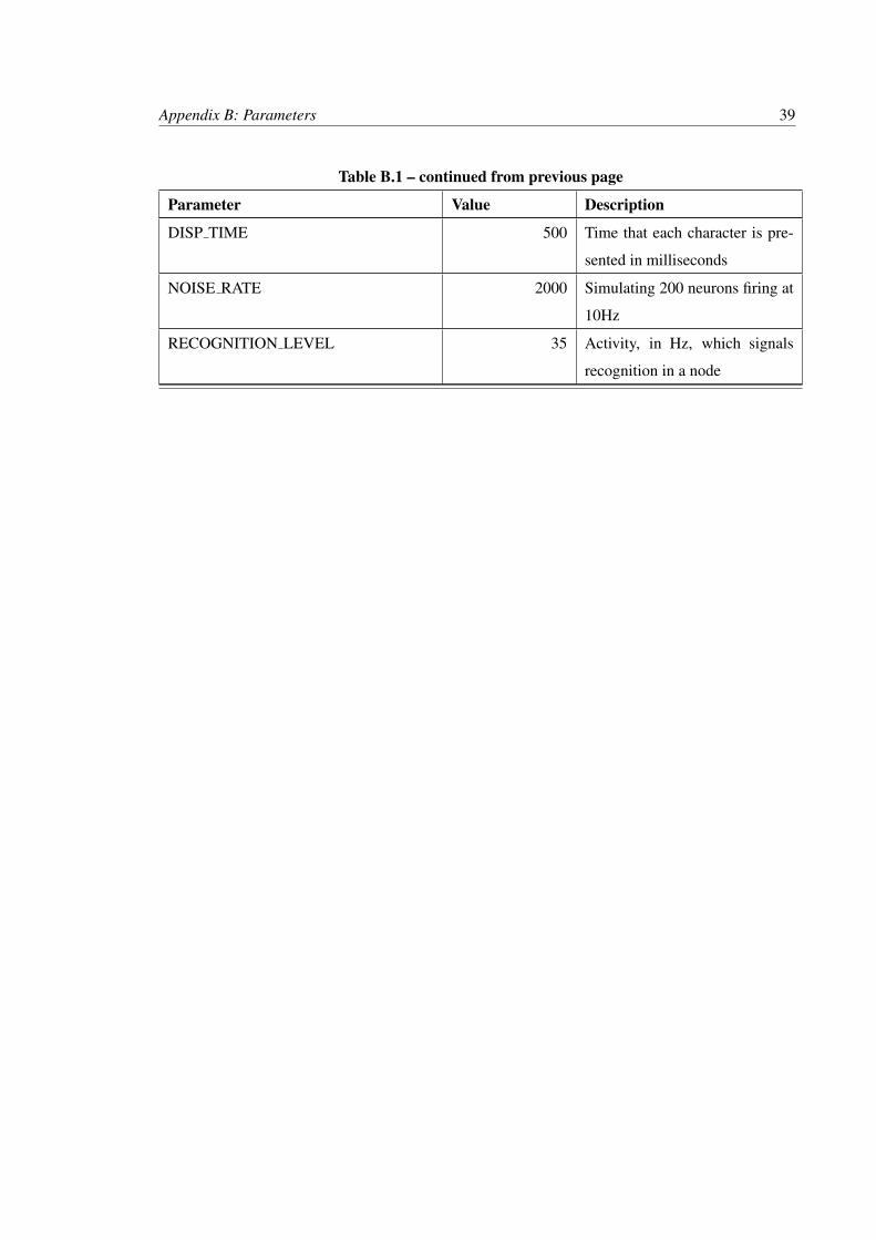
Appendix B: Parameters 39
Table B.1 – continued from previous page
Parameter Value Description
DISP TIME 500 Time that each character is pre-
sented in milliseconds
NOISE RATE 2000 Simulating 200 neurons firing at
10Hz
RECOGNITION LEVEL 35 Activity, in Hz, which signals
recognition in a node
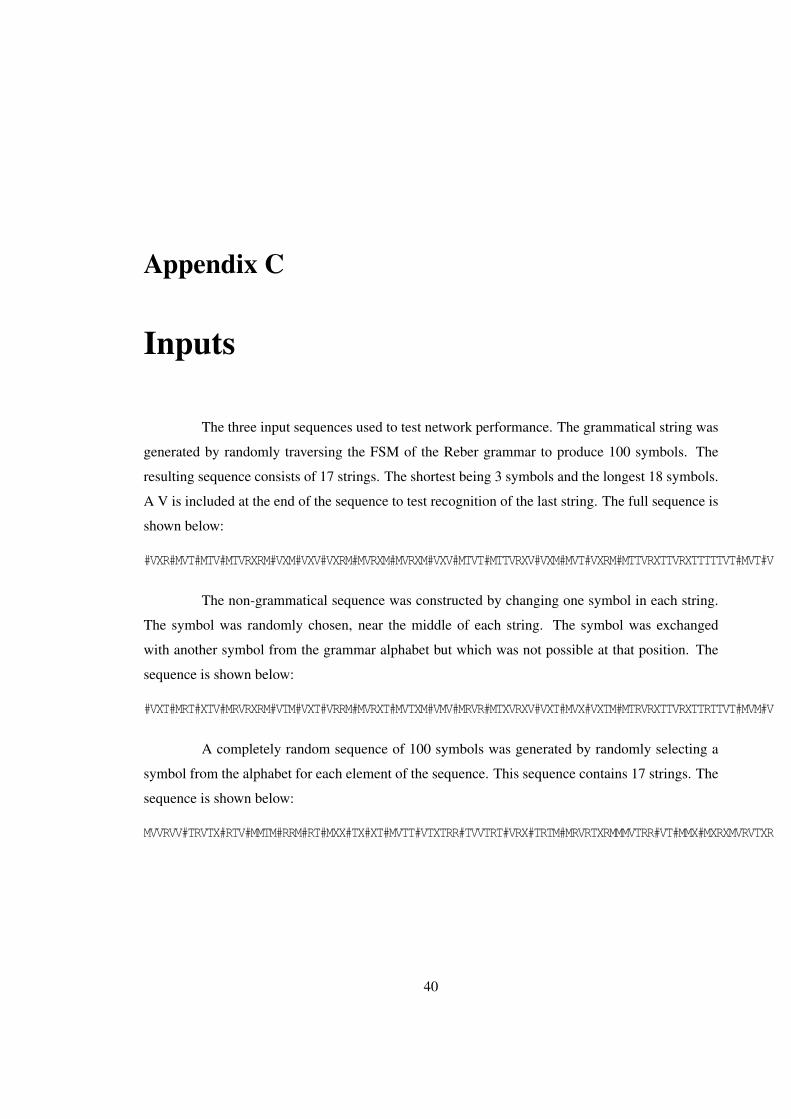
Appendix C
Inputs
The three input sequences used to test network performance. The grammatical string was
generated by randomly traversing the FSM of the Reber grammar to produce 100 symbols. The
resulting sequence consists of 17 strings. The shortest being 3 symbols and the longest 18 symbols.
A V is included at the end of the sequence to test recognition of the last string. The full sequence is
shown below:
#VXR#MVT#MTV#MTVRXRM#VXM#VXV#VXRM#MVRXM#MVRXM#VXV#MTVT#MTTVRXV#VXM#MVT#VXRM#MTTVRXTTVRXTTTTTVT#MVT#V
The non-grammatical sequence was constructed by changing one symbol in each string.
The symbol was randomly chosen, near the middle of each string. The symbol was exchanged
with another symbol from the grammar alphabet but which was not possible at that position. The
sequence is shown below:
#VXT#MRT#XTV#MRVRXRM#VTM#VXT#VRRM#MVRXT#MVTXM#VMV#MRVR#MTXVRXV#VXT#MVX#VXTM#MTRVRXTTVRXTTRTTVT#MVM#V
A completely random sequence of 100 symbols was generated by randomly selecting a
symbol from the alphabet for each element of the sequence. This sequence contains 17 strings. The
sequence is shown below:
MVVRVV#TRVTX#RTV#MMTM#RRM#RT#MXX#TX#XT#MVTT#VTXTRR#TVVTRT#VRX#TRTM#MRVRTXRMMMVTRR#VT#MMX#MXRXMVRVTXR
40