phc 6052 sas skills page 1 - university of...

PHC 6052 SAS Skills

General SAS Skills and Knowledge:

• SAS Windows (Program, Log, Output, Results, Explorer)

• SAS Menus (Open files, Submit files, View windows)

• Clearing SAS Windows (Log and Output)

• Creating and using a SAS library

• Working with SAS datasets in a library

• Working with SAS datasets in the work directory

• Viewing the contents of a SAS dataset using PROC CONTENTS proc contents data=bio.whas500; run;

proc contents data=bio.whas500 varnum; ods select position; run;

• Viewing the contents of a SAS dataset using PROC PRINT proc print data=bio.whas500; run;

proc print data=bio.whas500 (obs=10); var hr gender cvd year; run;

• Sorting a dataset using PROC SORT proc sort data=bio.whas500; by hr; run;

• Creating new datasets, new variables, and labeling variables using a DATA step data library.new; set library.old; var4 = var1/100; var5 = var2*1000; if 0 <= var4 <= 1.6 then var6 = 0; if var4 > 1.6 then var6 = 1; label var1="Height (cm)" var2="Weight (kg)" var3="Gender" var4="Height (m)" var5="Weight (g)" var6="Height Over 1.6 m?"; run;

• Create and clear custom titles /* Create your own title */ title 'My Title'; /* Clear all Default Titles */ title;

PHC 6052 SAS Skills

• Using ODS RTF and ODS PDF to export output to common formats

o Basic commands: (If this doesn’t work specify the file name and open the file manually)

ods pdf; /* SAS code for which output is requested */ ods pdf close; ods rtf; /* SAS code for which output is requested */ ods rtf close;

o More advanced examples: ods pdf notoc file="C:\MySAS\output.pdf"; /* SAS code for which output is requested */ ods pdf close; ods rtf bodytitle file="C:\MySAS\output.rtf"; /* SAS code for which output is requested */ ods rtf close;

• Using ODS GRAPHICS to obtain additional graphs from common analyses (this may or may not be needed in SAS 9.3 and beyond – try and see)

Note: Throughout we have included the ods graphics on/off command when they produce useful output in SAS 9.2. Most readers should now be using SAS version 9.3 or higher which, by default, provide ods graphics without the need for these commands and, in that case, they can usually be ignored.

ods graphics on; /* SAS Procedures */ ods graphics off;

PHC 6052 SAS Skills

Advanced SAS Skills:

• Common SAS options: Options nodate nonumber;

• Using PROC FORMAT and the FORMAT statement in a DATA step to associate a user defined format with a variable in a dataset

proc format; value YesNoFmt 1='Yes' 0='No'; value Sex01Ft 0='Male' 1='Female'; value yr 1='1997' 2='1999' 3='2001'; run; data WHAS500_formatted; set whas500_unformatted; format Gender Sex0Fmt. cvd afb sho chf av3 YesNoFmt. year yr.; run;

• Using ODS TRACE/SELECT/EXCLUDE to obtain only needed output ods trace on; /* SAS Procedures */ ods trace off;

• Adding text to ODS Output /* Add Text to RTF output For PDF output change the rtf below to pdf */

ods escapechar='^'; ods rtf text='^S={just=center font=("Times Roman",22PT,Bold)}

Descriptive Statistics using SAS'; • Adjusting graph sizes for ODS graphics

ods graphics / width=5in height=4in;

• Using the INSET statement in PROG SGPLOT and other advanced graphics topics • Using a WHERE statement in a PROC step to analyze a subset of the data

where 40 <= diasbp <= 120;

PHC 6052 SAS Skills

Descriptive Methods – One Categorical Variable

• Frequency distributions and bar charts using PROC FREQ ods graphics on; proc freq data=bio.whas500; tables gender; run; ods graphics off;

Multiple variables can be used in a given tables statement as in the example below: proc freq data=bio.whas500; tables afb sho chf year; /* List variables separated by spaces */ run;

PHC 6052 SAS Skills

Descriptive Methods – One Quantitative Variable

• Histograms using PROC SGPLOT proc sgplot data=bio.whas500; histogram hr; /* can only have one variable in HISTOGRAM statement */ run;

Normal or non-parametric (kernel) density estimates can be added using the DENSITY statement proc sgplot data=bio.whas500; histogram hr; density hr / type=normal; density hr / type=kernel; run;

PHC 6052 SAS Skills

• Histograms using PROC UNIVARIATE (density curves can also be added but generally SGPLOT is preferred for this)

proc univariate data=bio.whas500 noprint; /* NOPRINT = No text output*/ var hr age; histogram; run;

PHC 6052 SAS Skills

• Boxplots using PROC SGPLOT proc sgplot data=bio.whas500; vbox hr; /* VBOX for Vertical Boxplots */ run; proc sgplot data=bio.whas500; hbox hr; /* HBOX for Horizontal Boxplots */ run;

• Summary statistics using PROC MEANS

/* Default Summary Statistics */ proc means data=bio.whas500; var hr; /* can have more than one variable in the VAR statement */ run;

/* Requesting different Summary Statistics */ proc means data=bio.whas500 min q1 median q3 max fw=7 maxdec=2; var hr; run;

PHC 6052 SAS Skills

• Summary statistics using PROC UNIVARIATE (lengthy output) proc univariate data=bio.whas500 all; /* ALL option requests all UNIVARIATE output possible */ var hr; /* can have more than one variable in the VAR statement */ run;

The UNIVARIATE Procedure Variable: hr (Initial Heart Rate)

Moments

N 500 Sum Weights 500

Mean 87.018 Sum Observations 43509

Std Deviation 23.5862311 Variance 556.310297

Skewness 0.56676662 Kurtosis 0.47176453

Uncorrected SS 4063665 Corrected SS 277598.838

Coeff Variation 27.1050025 Std Error Mean 1.05480832

Basic Statistical Measures

Location Variability

Mean 87.0180 Std Deviation 23.58623

Median 85.0000 Variance 556.31030

Mode 100.0000 Range 151.00000

Interquartile Range 31.50000

Modes

Mode Count

100 16

Basic Confidence Limits Assuming Normality

Parameter Estimate 95% Confidence Limits

Mean 87.01800 84.94559 89.09041

Std Deviation 23.58623 22.20935 25.14650

Variance 556.31030 493.25519 632.34644

Tests for Location: Mu0=0

Test Statistic p Value

Student's t t 82.49651 Pr > |t| <.0001

Sign M 250 Pr >= |M| <.0001

Signed Rank S 62625 Pr >= |S| <.0001

Location Counts: Mu0=0.00

Count Value

Num Obs > Mu0 500

Num Obs ^= Mu0 500

Num Obs < Mu0 0

PHC 6052 SAS Skills

Tests for Normality

Test Statistic p Value

Shapiro-Wilk W 0.980406 Pr < W <0.0001

Kolmogorov-Smirnov D 0.049799 Pr > D <0.0100

Cramer-von Mises W-Sq 0.278942 Pr > W-Sq <0.0050

Anderson-Darling A-Sq 1.971014 Pr > A-Sq <0.0050

Trimmed Means

Percent Trimmed

in Tail

Number Trimmed

in Tail Trimmed

Mean

Std Error Trimmed

Mean 95% Confidence Limits DF t for H0:

Mu0=0.00 Pr > |t|

25.00 125 85.20000 1.139391 82.95593 87.44407 249 74.77676 <.0001

Winsorized Means

Percent Winsorized

in Tail

Number Winsorized

in Tail Winsorized

Mean

Std Error Winsorized

Mean 95% Confidence Limits DF t for H0:

Mu0=0.00 Pr > |t|

25.00 125 84.85000 1.140535 82.60367 87.09633 249 74.39492 <.0001

Robust Measures of Scale

Measure Value Estimate of Sigma

Interquartile Range 31.50000 23.35098

Gini's Mean Difference 26.37960 23.37831

MAD 16.00000 23.72160

Sn 23.85200 23.85200

Qn 22.21900 22.05141

Quantiles (Definition 5)

Quantile Estimate

Order Statistics

95% Confidence Limits Assuming Normality

95% Confidence Limits Distribution Free LCL Rank UCL Rank Coverage

100% Max 186.0

99% 150.0 138.1125 146.1037 146 186 491 500 96.23

95% 128.5 122.7901 129.1550 123 139 466 486 95.89

90% 117.0 114.5712 120.1696 114 121 437 464 95.63

75% Q3 100.5 100.6978 105.2915 99 105 357 395 95.01

50% Median 85.0 84.9456 89.0904 83 88 229 273 95.08

25% Q1 69.0 68.7445 73.3382 67 72 106 144 95.01

10% 59.0 53.8664 59.4648 57 61 37 64 95.63

5% 54.0 44.8810 51.2459 47 56 15 35 95.89

1% 42.0 27.9323 35.9235 35 45 1 10 96.23

0% Min 35.0

PHC 6052 SAS Skills

Extreme Observations

Lowest Highest

Value Obs Value Obs

35 1 150 496

36 3 154 497

36 2 157 498

38 4 160 499

42 7 186 500

Extreme Values

Lowest Highest

Order Value Freq Order Value Freq

1 35 1 101 150 3

2 36 2 102 154 1

3 38 1 103 157 1

4 42 3 104 160 1

5 44 1 105 186 1

Frequency Counts

Value Count

Percents

Cell Cum

35 1 0.2 0.2

36 2 0.4 0.6

38 1 0.2 0.8

42 3 0.6 1.4

44 1 0.2 1.6

All Observed Data Values

148 1 0.2 98.4

149 1 0.2 98.6

150 3 0.6 99.2

154 1 0.2 99.4

157 1 0.2 99.6

160 1 0.2 99.8

186 1 0.2 100.0

PHC 6052 SAS Skills

Histogram # Boxplot 185+* 1 0 . .* 1 0 155+*** 5 0 .**** 7 0 .***** 10 | 125+********** 19 | .********************* 41 | .***************************** 57 +-----+ 95+************************************* 73 | | .******************************************** 87 *--+--* .*********************************** 70 | | 65+*************************************** 78 +-----+ .****************** 35 | .****** 12 | 35+** 4 | ----+----+----+----+----+----+----+----+---- * may represent up to 2 counts Normal Probability Plot 185+ * | | * 155+ **** | ****+++ | ***+++ 125+ ****+ | ***** | ***** 95+ ***** | ****** | +**** 65+ ******* | ******+ | ******+++ 35+**++++ +----+----+----+----+----+----+----+----+----+----+ -2 -1 0 +1 +2

PHC 6052 SAS Skills

Descriptive Methods – One Quantitative and One Categorical Variable

• Boxplots of the quantitative variable by the categorical variable using PROC SGPLOT (similar results can be obtained using HBOX)

proc sgplot data=bio.whas500; vbox hr / category=cvd; /* can only have 1 variable in VBOX statement*/ run;

proc sgplot data=bio.whas500; vbox age / category=gender; run;

PHC 6052 SAS Skills

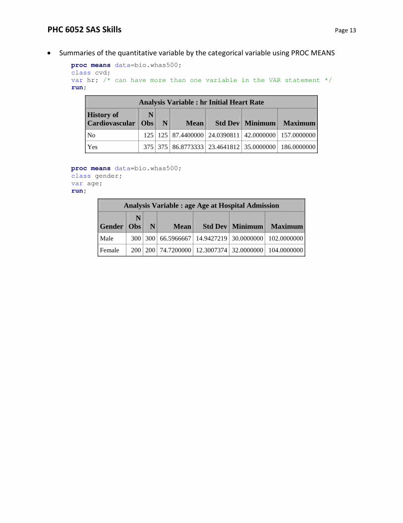
• Summaries of the quantitative variable by the categorical variable using PROC MEANS proc means data=bio.whas500; class cvd; var hr; /* can have more than one variable in the VAR statement */ run;

proc means data=bio.whas500; class gender; var age; run;

Analysis Variable : hr Initial Heart Rate

History of Cardiovascular

N Obs N Mean Std Dev Minimum Maximum

No 125 125 87.4400000 24.0390811 42.0000000 157.0000000

Yes 375 375 86.8773333 23.4641812 35.0000000 186.0000000

Analysis Variable : age Age at Hospital Admission

Gender N

Obs N Mean Std Dev Minimum Maximum Male 300 300 66.5966667 14.9427219 30.0000000 102.0000000

Female 200 200 74.7200000 12.3007374 32.0000000 104.0000000

PHC 6052 SAS Skills

Descriptive Methods – Two Categorical Variables

• Two-Way Tables (Contingency Tables) using PROC FREQ ods graphics on; proc freq data=bio.whas500; tables gender*cvd; run; ods graphics off;

ods graphics on; proc freq data=bio.whas500; tables cvd*gender; run; ods graphics off;

PHC 6052 SAS Skills

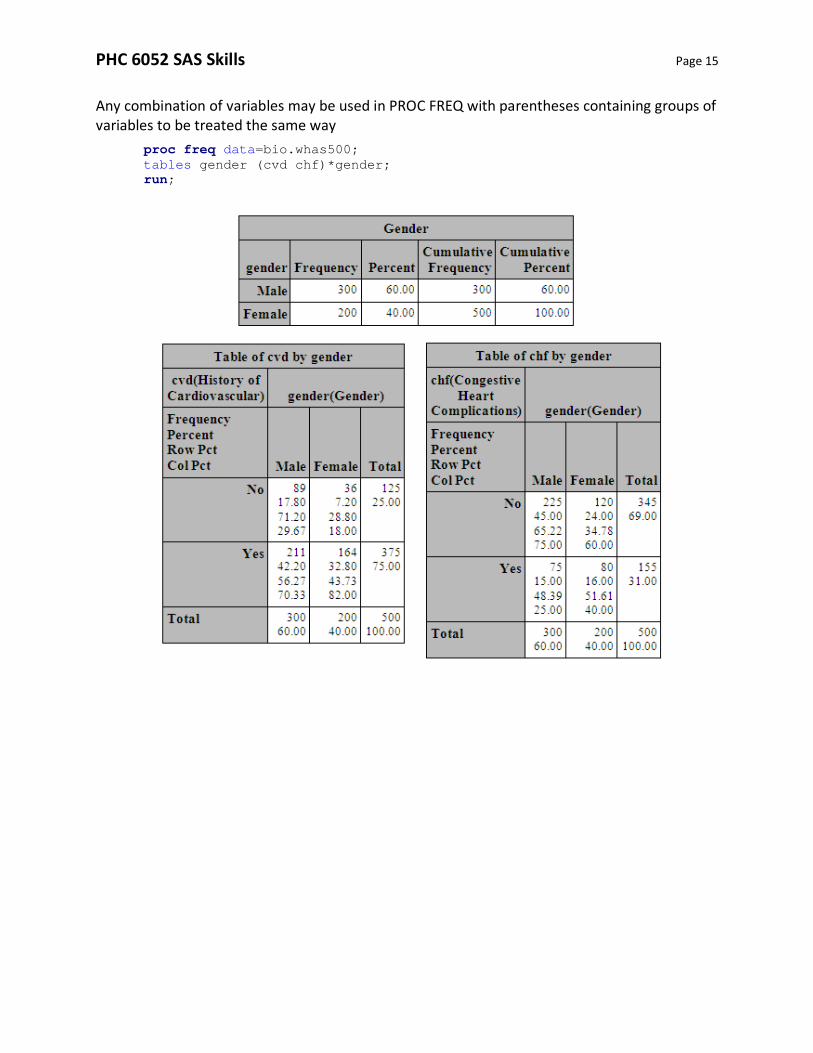
Any combination of variables may be used in PROC FREQ with parentheses containing groups of variables to be treated the same way

proc freq data=bio.whas500; tables gender (cvd chf)*gender; run;

PHC 6052 SAS Skills

Descriptive Methods – Two Quantitative Variables

• Scatterplots using PROC SGPLOT proc sgplot data=bio.whas500; scatter y=diasbp x=sysbp; /* Only one plot per SGPLOT

Can overlay plots */ run;

• Scatterplots with LOESS smoothed trend line using PROC SGPLOT

proc sgplot data=bio.whas500; loess y=diasbp x=sysbp / smooth=0.3; /* smooth ranges from

0=no smoothing to 1=linear */ run;

PHC 6052 SAS Skills

• Calculate Pearson’s correlation coefficient (only meaningful for approximately linear trend) ods graphics on; proc corr data=bio.whas500 plots=matrix(histogram); var diasbp sysbp; run; ods graphics off;

PHC 6052 SAS Skills

• Adding information about a categorical variable to a scatterplot proc sgplot data=bio.whas500; where 40 <= diasbp <= 120; loess y=hr x=diasbp / group=chf smooth=0.5; run;

PHC 6052 SAS Skills

Inferential Statistics – Investigating Normality

• Normal probability plots using PROC UNIVARIATE ods graphics on; proc univariate data=bio.whas500 noprint; var hr age; qqplot / normal(mu=est sigma=est); run; ods graphics off;

• Common tests of normality using PROC UNIVARIATE

proc univariate data=bio.whas500 normaltest; var hr age; ods select testsfornormality; run;

PHC 6052 SAS Skills

Inferential Statistics – One Sample – Binomial Proportion

• Tests and Intervals for one binomial proportion using PROC FREQ. The following conducts a test of the null hypothesis that the proportion of congestive heart complications in the population is 25%. Confidence intervals are also provided via this output.

proc freq data=bio.whas500; tables chf / binomial(level="Yes" p=0.25); run;

PHC 6052 SAS Skills

• Power calculations for one binomial proportion using PROC POWER proc power; onesamplefreq test=z method=normal proportion = .30 nullproportion = .25 ntotal = 100 alpha = 0.05 sides = 1 power=.; run;

• Sample size calculations for one binomial proportion using PROC POWER

proc power; onesamplefreq test=z method=normal proportion = .30 nullproportion = .25 ntotal = . alpha = 0.05 sides = 1 power=.90; run;

PHC 6052 SAS Skills

Inferential Statistics – One Sample – Quantitative Variable

• T-tests and confidence intervals for the mean of a normally distributed population using PROC TTEST (confidence intervals for the standard deviation of the population are also reported)

ods graphics on; proc ttest data=bio.whas500 h0=80; var hr; run; ods graphics off;

PHC 6052 SAS Skills

• T-tests and confidence intervals for the mean of a normally distributed population using PROC UNIVARIATE (confidence intervals for the standard deviation and variance of the population are also reported)

proc univariate data=bio.whas500 mu0=80 cibasic; var hr; ods select testsforlocation basicintervals; run;

• Power calculations for one sample t-tests using PROC POWER

proc power; onesamplemeans test=t dist=normal mean = 30 nullmean = 28 ntotal = 100 alpha = 0.05 sides = 1 std = 6 power=.; run;

PHC 6052 SAS Skills

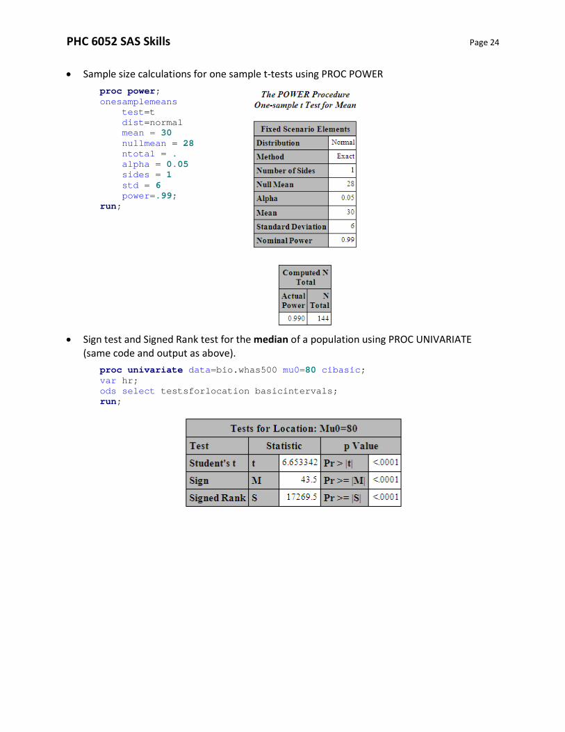
• Sample size calculations for one sample t-tests using PROC POWER proc power; onesamplemeans test=t dist=normal mean = 30 nullmean = 28 ntotal = . alpha = 0.05 sides = 1 std = 6 power=.99; run;

• Sign test and Signed Rank test for the median of a population using PROC UNIVARIATE (same code and output as above).

proc univariate data=bio.whas500 mu0=80 cibasic; var hr; ods select testsforlocation basicintervals; run;

PHC 6052 SAS Skills

• Power graphs using PROC POWER (can be requested for any design, not just onesamplemeans)

proc power; onesamplemeans test=T dist=normal power=. ntotal=500 nullmean=80 mean=83 85 87 std= 24 28 32; plot x=effect; run;

proc power; onesamplemeans test=T dist=normal power=0.8 ntotal=. nullmean=80 mean=83 85 87 std= 24 28 32; plot x=effect; run;

83 84 85 86 87

Mean

0.5

0.6

0.7

0.8

0.9

1.0

Pow

er

Std Dev 242832

83 84 85 86 87

Mean

0100200300400500600700800900

Tota

l Sam

ple

Size

Std Dev 242832

PHC 6052 SAS Skills

Inferential Statistics – Paired Samples – Quantitative Variable

• For the following we use the data below, entered into SAS directly using a DATA step data example; input jan apr; diff=jan-apr; datalines; 139 104 122 113 126 100 64 88 78 61 run;

• Paired t-tests using PROC TTEST and the PAIRED statement ods graphics on; proc ttest data=example; paired jan*apr; run; ods graphics off;

PHC 6052 SAS Skills

• Paired t-tests using PROC UNIVARIATE (this code also conducts the sign test and signed rank test for paired samples). I have requested tests for normality as well.

proc univariate data=example cibasic normaltest; var diff; ods select basicintervals testsforlocation testsfornormality; run;

PHC 6052 SAS Skills

Inferential Statistics – Two Independent Samples – Quantitative Variable

• Comparing means of two independent samples from normal populations using PROC TTEST ods graphics on; proc ttest data=bio.whas500; class gender; var hr sysbp bmi; run; ods graphics off;

PHC 6052 SAS Skills

PHC 6052 SAS Skills

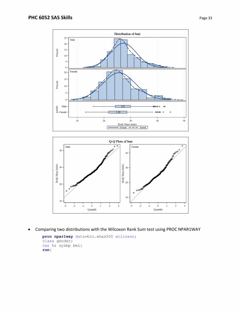
• Comparing two distributions with the Wilcoxon Rank Sum test using PROC NPAR1WAY proc npar1way data=bio.whas500 wilcoxon; class gender; var hr sysbp bmi; run;

PHC 6052 SAS Skills

PHC 6052 SAS Skills

• Obtaining the exact p-value for the Wilcoxon Rank Sum test using PROC NPAR1WAY (only the 2nd table – of three – is provided below, the rest remains the same)

data smallsamp; set bio.whas500; where sho=1; /* keep only 22 obs. with cardiogenic shock */ run; proc npar1way data=smallsamp wilcoxon; class gender; var hr; exact wilcoxon; run;

PHC 6052 SAS Skills

Inferential Statistics – Two Categorical Variables

• Chi-square and Fisher’s exact tests for association or equality of two proportions (2x2 tables)

proc freq data=bio.whas500; table gender*(cvd afb) / chisq riskdiff ; run;

PHC 6052 SAS Skills

PHC 6052 SAS Skills

• Chi-square and Fisher’s exact tests for association (RxC tables). Fisher’s exact test must be requested in this case.

proc freq data=bio.whas500; table gender*year / chisq fisher ; run;

• McNemar’s tests for paired proportions. Consider a test for high blood pressure (Y/N) at baseline and again at 6 months.

data mcnemar; input ID HBP0 HBP1 @@; label HBP0 = "High BP at Baseline" HBP1 = "High BP at 6 Mo."; datalines; 1 0 0 2 1 1 3 1 0 4 1 1 5 1 1 6 0 0 7 0 0 8 0 0 9 0 0 10 1 1 11 0 0 12 1 1 13 1 1 14 1 1 15 0 0 16 1 1 17 0 0 18 1 1 19 0 1 20 0 0 21 0 1 22 1 1 23 1 0 24 0 0 25 0 0 26 1 0 27 0 0 28 0 0 29 0 0 30 1 0 31 0 1 32 0 0 33 1 0 34 1 0 35 1 1 36 0 0 37 1 1 38 0 0 39 0 0 40 0 0 41 1 1 42 0 0 43 0 1 44 1 1 45 0 0 46 0 0 47 0 0 48 1 1 49 0 0 50 1 0 51 0 0 52 0 0 53 0 0 54 1 1 55 1 0 56 1 1 57 0 0 58 1 1 59 0 0 60 0 1 61 0 0 62 1 1 63 1 0 64 0 0 65 1 0 66 0 0 67 1 0 68 0 0 69 1 0 70 1 1 71 1 0 72 0 0 73 0 0 74 0 1 75 0 0 76 0 0 77 0 0 78 1 1 79 1 0 80 1 0 81 1 1 82 0 0 83 1 0 84 0 0 85 0 0 86 1 0 87 1 0 88 0 0 89 1 1 90 0 0 91 0 0 92 0 0 93 1 1 94 0 0 95 1 0 96 1 0 ; run;

PHC 6052 SAS Skills

proc freq data=mcnemar; tables HBP0*HBP1 / agree; exact mcnem; run;

PHC 6052 SAS Skills

Inferential Statistics – Two Quantitative Variables

• Tests and confidence intervals for the population correlation coefficient using PROC CORR. Using the VAR statement alone computes for all possible pairs. Using the VAR and WITH statements produces only combinations with one variable from each statement.

ods graphics on; proc corr data=bio.whas500 plots=matrix(histogram) fisher; var diasbp sysbp age ; run; ods graphics off;

PHC 6052 SAS Skills

PHC 6052 SAS Skills

Using VAR and WITH proc corr data=bio.whas500 fisher; var diasbp age ; with sysbp ; run;

Spearman Rank Correlation: proc corr data=bio.whas500 spearman; var diasbp sysbp ; run;

PHC 6052 SAS Skills

• Simple linear regression using PROC REG

Continuous Predictor ods graphics on; proc reg data=bio.whas500; model sysbp = diasbp; run; quit; ods graphics off;

PHC 6052 SAS Skills

PHC 6052 SAS Skills

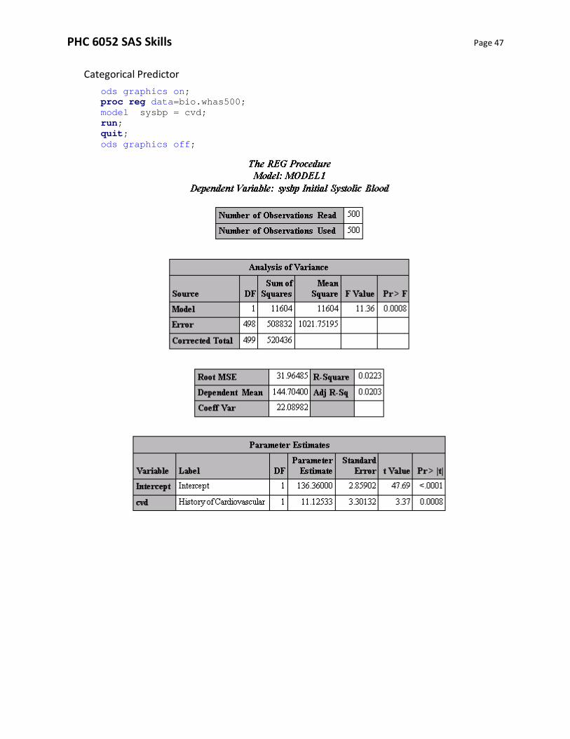
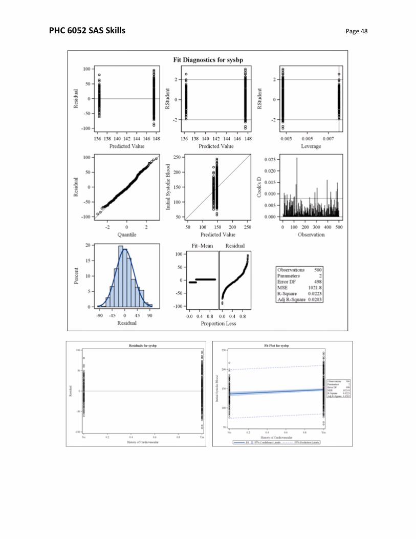
Categorical Predictor ods graphics on; proc reg data=bio.whas500; model sysbp = cvd; run; quit; ods graphics off;

PHC 6052 SAS Skills

PHC 6052 SAS Skills

Equivalent tests with continuous outcome and bivariate predictor proc ttest data=bio.whas500; class cvd; var sysbp; run;

proc corr data=bio.whas500; var cvd ; with sysbp; run;

PHC 6052 SAS Skills

Inferential Statistics – Multiple Linear Regression

• Using PROC REG ods graphics on; proc reg data=bio.whas500; model sysbp = diasbp age gender cvd ; run; quit; ods graphics off;

PHC 6052 SAS Skills

PHC 6052 SAS Skills

Inferential Statistics – Additional Topics

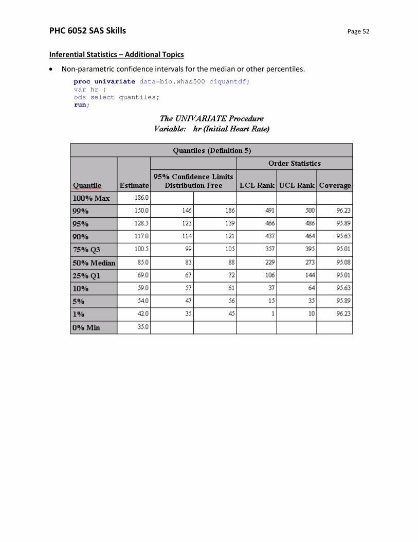
• Non-parametric confidence intervals for the median or other percentiles. proc univariate data=bio.whas500 ciquantdf; var hr ; ods select quantiles; run;

phc 6052 sas skills page 1 - university of...

Documents