phase-space description of charged particle beams
TRANSCRIPT
Phase-space Description of Charged Particle Beams
Fall, 2017
Kyoung-Jae Chung
Department of Nuclear Engineering
Seoul National University

2/18 Radiation Source Engineering, Fall 2017
Basic properties of electron and proton
Electron (e)• Mass (me) = 9.11x10⁻³¹ kg• Charge (qe) = -1.6x10⁻¹⁹ C (-e)• Rest energy = 0.511 MeV• Electrons are relativistic when they have kinetic energy above about 100
keV.
Proton (p, H+)• Mass (mp) = 1.67x10⁻²⁷ kg mi = Amp (A: atomic mass number)• Charge (qp) = +1.6x10⁻¹⁹ C (+e) qi = Z*qp (Z*: charge state of the ion)• Rest energy = 938.27 MeV• Because of the high rest energy, we can use Newtonian dynamics to predict
the motion of ions in many applications.

3/18 Radiation Source Engineering, Fall 2017
Beam
Although single charged particles may be useful for some physics experiments, we need large numbers of energetic particles for most applications. A flux of particles is a beam when the following two conditions hold:
• The particles travel in almost the same direction.• The particles have a small spread in kinetic energy.
A beam is an ordered flow of charged particles. A disordered set of particles, such as a thermal plasma, is not a beam.
The degree of order in a flow of particles is called coherence.
4/18 Radiation Source Engineering, Fall 2017
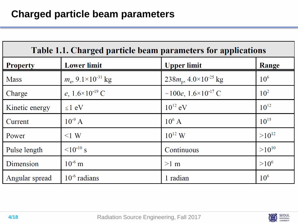
Charged particle beam parameters
5/18 Radiation Source Engineering, Fall 2017
Description of particle dynamics
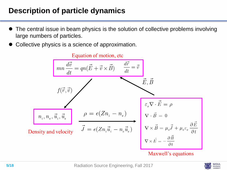
The central issue in beam physics is the solution of collective problems involving large numbers of particles.
Collective physics is a science of approximation.

6/18 Radiation Source Engineering, Fall 2017
Particle dynamics
The special theory of relativity states that the inertia of a particle observed in a frame of reference depends on the magnitude of its speed in that frame.
The inertia of a particle is proportional to 𝛾𝛾. The apparent mass is 𝑚𝑚 = 𝛾𝛾𝑚𝑚0. The particle momentum, a vector quantity, equals 𝒑𝒑 = 𝛾𝛾𝑚𝑚0𝒗𝒗. The equation of motion:
The kinetic energy equals the total energy minus the rest energy:
Newtonian dynamics describes the motion of low-energy particles when 𝑇𝑇 ≪𝑚𝑚0𝑐𝑐2.
𝛾𝛾 =1
1 − 𝑣𝑣/𝑐𝑐 2=
11 − 𝛽𝛽2
𝑑𝑑𝒑𝒑𝑑𝑑𝑑𝑑 =
𝑑𝑑(𝛾𝛾𝑚𝑚0𝒗𝒗)𝑑𝑑𝑑𝑑 = 𝑭𝑭
𝑇𝑇 = 𝛾𝛾 − 1 𝑚𝑚0𝑐𝑐2
Lorentz factor

7/18 Radiation Source Engineering, Fall 2017
Transfer matrix
Most beam transport devices, such as charged particle lenses and bending magnets, apply transverse forces that are linearly proportional to the distance of a particle from a preferred axis.
To specify the orbit of the particle in the x-direction, we must give its position, x, and velocity, vx. The convention in charged-particle optics is to represent particle orbits in terms of their angle relative to the main axis, rather than the transverse velocity. In the limit that 𝑣𝑣𝑥𝑥 ≪ 𝑣𝑣𝑧𝑧, the angle is
If the x-directed forces in the device are linear, then we can express the exit vector as a linear combination of the entrance vector components:
The quantities amn depend on the distribution of forces. Without acceleration, the determinant of the transfer matrix equals unity.
𝑥𝑥′ =𝑑𝑑𝑥𝑥𝑑𝑑𝑑𝑑
≈𝑣𝑣𝑥𝑥𝑣𝑣𝑧𝑧
𝑥𝑥1𝑥𝑥1′
=𝑎𝑎11 𝑎𝑎12𝑎𝑎21 𝑎𝑎22
𝑥𝑥0𝑥𝑥0′
Transfer matrixExit vector Entrance vector

8/18 Radiation Source Engineering, Fall 2017
Transfer matrix
If a particle travels through linear device A and then through device B, the final orbit vector is
The orbit vector transformation from any combination of one-dimensional focusing elements is a single transfer matrix, the product of the individual matrices of all the elements.
The particle orbit vector for a two-dimensional focusing system is 𝒙𝒙 = [𝑥𝑥, 𝑥𝑥𝑥,𝑦𝑦,𝑦𝑦𝑥]. A 4×4 matrix represents the effect of a general linear focusing element or system.
In many practical devices, such as quadrupole lens arrays, the forces in the 𝑥𝑥and 𝑦𝑦 directions are independent. Then, we can calculate motion in 𝑥𝑥 and 𝑦𝑦separately using individual 2×2 matrices.
𝑥𝑥2𝑥𝑥2′
= 𝑏𝑏11 𝑏𝑏12𝑏𝑏21 𝑏𝑏22
𝑎𝑎11 𝑎𝑎12𝑎𝑎21 𝑎𝑎22
𝑥𝑥0𝑥𝑥0′
𝒙𝒙𝟐𝟐 = 𝑩𝑩 𝑨𝑨𝒙𝒙𝟎𝟎 = 𝑩𝑩𝑨𝑨 𝒙𝒙𝟎𝟎 = 𝑪𝑪𝒙𝒙𝟎𝟎
9/18 Radiation Source Engineering, Fall 2017
Phase dynamics
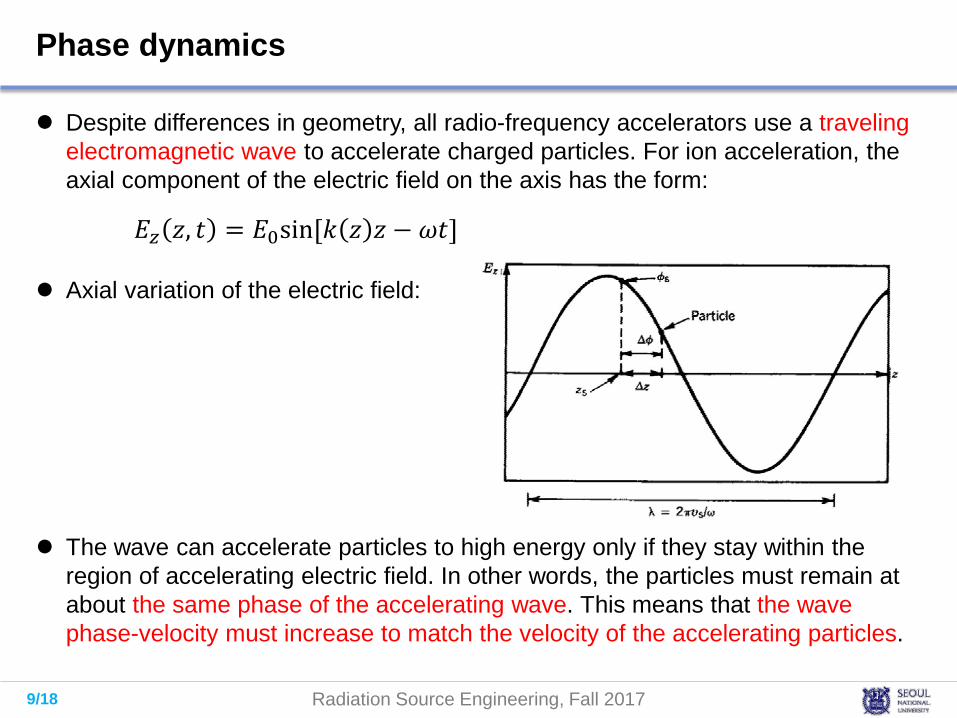
Despite differences in geometry, all radio-frequency accelerators use a traveling electromagnetic wave to accelerate charged particles. For ion acceleration, the axial component of the electric field on the axis has the form:
Axial variation of the electric field:
The wave can accelerate particles to high energy only if they stay within the region of accelerating electric field. In other words, the particles must remain at about the same phase of the accelerating wave. This means that the wave phase-velocity must increase to match the velocity of the accelerating particles.
𝐸𝐸𝑧𝑧 𝑑𝑑, 𝑑𝑑 = 𝐸𝐸0sin[𝑘𝑘 𝑑𝑑 𝑑𝑑 − 𝜔𝜔𝑑𝑑]

10/18 Radiation Source Engineering, Fall 2017
Synchronous particle
The wave accelerates particles with phase in the range 0 < 𝜙𝜙 < 𝜋𝜋 and decelerates particles in the phase range −𝜋𝜋 < 𝜙𝜙 < 0 .
𝑑𝑑𝑣𝑣𝑠𝑠 𝑑𝑑𝑑𝑑𝑑𝑑
=𝑞𝑞𝐸𝐸0 sin𝜙𝜙𝑠𝑠
𝑚𝑚0
We can define conditions where a particle stays at a constant phase. A particle with this property is a synchronous particle – its phase is the synchronous phase, 𝜙𝜙𝑠𝑠.
Figure shows that the synchronous particle experiences a constant axial electric field, 𝐸𝐸𝑧𝑧𝑠𝑠 = 𝐸𝐸0 sin𝜙𝜙𝑠𝑠.
The velocity of the synchronous particle changes as:
The accelerating structure must vary along its length so that the wave number is 𝑘𝑘 𝑑𝑑 =
𝜔𝜔𝑣𝑣𝑠𝑠 𝑑𝑑
Conditions for having synchronous particles in an accelerator

11/18 Radiation Source Engineering, Fall 2017
Non-synchronous particle
Under some conditions non-synchronous particles have stable oscillations about the synchronous particle position, 𝑑𝑑𝑠𝑠.
Let 𝑑𝑑 and 𝑣𝑣 be the axial position and velocity of a non-synchronous particle. We define the small quantities:
Then, we obtain
The instantaneous acceleration of the non-synchronous particle is:
The general phase equations for non-relativistic particles:
𝑑𝑑2𝑑𝑑𝑑𝑑𝑑𝑑2
=𝑑𝑑𝑣𝑣𝑑𝑑𝑑𝑑
=𝑞𝑞𝐸𝐸0 sin𝜙𝜙
𝑚𝑚0
𝑑𝑑2∆𝑑𝑑𝑑𝑑𝑑𝑑2
=𝑞𝑞𝐸𝐸0 sin𝜙𝜙
𝑚𝑚0−𝑑𝑑2𝑑𝑑𝑠𝑠𝑑𝑑𝑑𝑑2
=𝑞𝑞𝐸𝐸0𝑚𝑚0
sin𝜙𝜙 − sin𝜙𝜙𝑠𝑠
𝜙𝜙 = 𝜙𝜙𝑠𝑠 − 𝜔𝜔∆𝑑𝑑/𝑣𝑣𝑠𝑠

12/18 Radiation Source Engineering, Fall 2017
Non-synchronous particle
If 𝐸𝐸0 and 𝑣𝑣𝑠𝑠 are almost constant during an axial oscillation of a non-synchronous particle, then we obtain a non-linear differential equation as following:
For small oscillations about the phase of the synchronous particle, ∆𝜙𝜙 ≪ 𝜙𝜙𝑠𝑠, the above equation reduces to:
If cos𝜙𝜙𝑠𝑠 > 0, the axial oscillations of non-synchronous particles are stable. The conditions for synchronized particle acceleration are cos𝜙𝜙𝑠𝑠 > 0 and sin𝜙𝜙𝑠𝑠 >
0, or
The conditions for synchronized particle deceleration are cos𝜙𝜙𝑠𝑠 > 0 and sin𝜙𝜙𝑠𝑠 <0, or
𝑑𝑑2𝜙𝜙𝑑𝑑𝑑𝑑2
≅ −𝜔𝜔𝑞𝑞𝐸𝐸0𝑚𝑚0𝑣𝑣𝑠𝑠
sin𝜙𝜙 − sin𝜙𝜙𝑠𝑠
𝑑𝑑2∆𝜙𝜙𝑑𝑑𝑑𝑑2
≅ −𝜔𝜔𝑞𝑞𝐸𝐸0𝑚𝑚0𝑣𝑣𝑠𝑠
cos𝜙𝜙𝑠𝑠 ∆𝜙𝜙
0 < 𝜙𝜙𝑠𝑠 < 𝜋𝜋/2 (acceleration)
−𝜋𝜋/2 < 𝜙𝜙𝑠𝑠 < 0 (deceleration)

13/18 Radiation Source Engineering, Fall 2017
Configuration space vs phase space
Lamina phase flow is the foundation for theories of collective behavior.
(𝑥𝑥(𝑑𝑑),𝑦𝑦(𝑑𝑑), 𝑑𝑑(𝑑𝑑))
(𝑥𝑥,𝑦𝑦, 𝑑𝑑, 𝑣𝑣𝑥𝑥, 𝑣𝑣𝑦𝑦, 𝑣𝑣𝑑𝑑)

14/18 Radiation Source Engineering, Fall 2017
Examples of phase space description
The trajectories of particles accelerated by a constant axial electric field 𝐸𝐸𝑑𝑑:
Trajectories of particles in a linear focusing force 𝐹𝐹𝑥𝑥 = −𝑎𝑎𝑥𝑥:
𝑑𝑑 𝑑𝑑 = 𝑑𝑑0 + 𝑣𝑣𝑧𝑧0𝑑𝑑 + ⁄𝑞𝑞𝐸𝐸𝑧𝑧 𝑚𝑚0 𝑑𝑑2/2
𝑣𝑣𝑧𝑧 𝑑𝑑 = 𝑣𝑣𝑧𝑧0 + ⁄𝑞𝑞𝐸𝐸𝑧𝑧 𝑚𝑚0 𝑑𝑑
𝑥𝑥 𝑑𝑑 = 𝑥𝑥0 cos(𝜔𝜔𝑑𝑑 + 𝜙𝜙)
𝜔𝜔 = 𝑎𝑎/𝑚𝑚0
𝑣𝑣𝑥𝑥 𝑑𝑑 = −𝑥𝑥0𝜔𝜔 sin(𝜔𝜔𝑑𝑑 + 𝜙𝜙)
300 keV protons with a betatron wavelength of 0.3 m
Protons in an electric field of 105 V/m
15/18 Radiation Source Engineering, Fall 2017
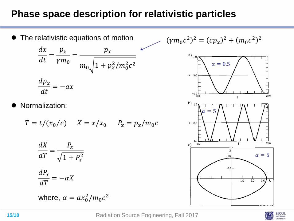
Phase space description for relativistic particles
The relativistic equations of motion
Normalization:
𝑑𝑑𝑥𝑥𝑑𝑑𝑑𝑑
=𝑝𝑝𝑥𝑥𝛾𝛾𝑚𝑚0
=𝑝𝑝𝑥𝑥
𝑚𝑚0 1 + 𝑝𝑝𝑥𝑥2/𝑚𝑚02𝑐𝑐2
𝑑𝑑𝑝𝑝𝑥𝑥𝑑𝑑𝑑𝑑
= −𝑎𝑎𝑥𝑥
𝛾𝛾𝑚𝑚0𝑐𝑐2 2 = 𝑐𝑐𝑝𝑝𝑥𝑥 2 + 𝑚𝑚0𝑐𝑐2 2
𝑑𝑑𝑑𝑑𝑑𝑑𝑇𝑇 =
𝑃𝑃𝑥𝑥1 + 𝑃𝑃𝑥𝑥2
𝑑𝑑𝑃𝑃𝑥𝑥𝑑𝑑𝑇𝑇 = −𝛼𝛼𝑑𝑑
where, 𝛼𝛼 = 𝑎𝑎𝑥𝑥02/𝑚𝑚0𝑐𝑐2
𝑇𝑇 = 𝑑𝑑/( ⁄𝑥𝑥0 𝑐𝑐) 𝑑𝑑 = 𝑥𝑥/𝑥𝑥0 𝑃𝑃𝑥𝑥 = 𝑝𝑝𝑥𝑥/𝑚𝑚0𝑐𝑐
𝛼𝛼 = 0.5
𝛼𝛼 = 5
𝛼𝛼 = 5

16/18 Radiation Source Engineering, Fall 2017
Conservation of phase space volume
Conservation of the phase-space volume occupied by a particle distribution is a fundamental theorem of collective physics. (Liouville’s theorem: the principle of incompressiblity of a phase fluid)
Same area

17/18 Radiation Source Engineering, Fall 2017
Maxwell distribution
Particles in an isotropic Maxwell distribution are in thermal equilibrium. They have a spread in kinetic energy.
For a single species in thermal equilibrium with itself (e.g. electrons), in the absence of time variation, spatial gradients, and accelerations, the Boltzmann equation reduces to
Then, we obtain the Maxwell-Boltzmann velocity distribution
𝑓𝑓 𝑣𝑣 =2𝜋𝜋
𝑚𝑚𝑘𝑘𝑇𝑇
3𝑣𝑣2𝑒𝑒𝑥𝑥𝑝𝑝 −
𝑚𝑚𝑣𝑣2
2𝑘𝑘𝑇𝑇
𝑓𝑓 𝜀𝜀 =2𝜋𝜋
𝜀𝜀𝑘𝑘𝑇𝑇
1/2𝑒𝑒𝑥𝑥𝑝𝑝 −
𝜀𝜀𝑘𝑘𝑇𝑇
The mean speed
�̅�𝑣 =8𝑘𝑘𝑇𝑇𝜋𝜋𝑚𝑚
1/2
�𝜕𝜕𝑓𝑓𝜕𝜕𝑑𝑑 𝑐𝑐
= 0

18/18 Radiation Source Engineering, Fall 2017
Displaced Maxwell distribution
Charged particle beams are non-isotropic and usually almost monoenergetic. In a sense, the primary goal of beam technology is to create non-Maxwelliandistributions and to preserve them over time scales set by the application.
A common assumption used in beam theory is that the particles have a Maxwell distribution when observed in the beam rest frame. The transformed distribution observed in the stationary frame of the accelerator is called a displaced Maxwell distribution.
For example, consider a nonrelativistic ion beam extracted from a plasma source with ion temperature 𝑇𝑇𝑖𝑖. The beam is axially bunched passing through a radio-frequency quadrupole accelerator. The beam emerges from the accelerator with kinetic energy 𝐸𝐸0. We can represent the exit beam distribution in the stationary frame as
𝑓𝑓 𝑣𝑣𝑥𝑥,𝑣𝑣𝑦𝑦 ,𝑣𝑣𝑧𝑧 ~ 𝑒𝑒𝑥𝑥𝑝𝑝 −𝑚𝑚𝑖𝑖(𝑣𝑣𝑥𝑥2 + 𝑣𝑣𝑦𝑦2)
2𝑘𝑘𝑇𝑇𝑖𝑖𝑒𝑒𝑥𝑥𝑝𝑝 −
𝑚𝑚𝑖𝑖(𝑣𝑣𝑧𝑧 − 𝑣𝑣0)2
2𝑘𝑘𝑇𝑇𝑖𝑖′
𝑣𝑣0 =2𝐸𝐸0𝑚𝑚𝑖𝑖
1/2