stochastic-hydrodynamic model of halo formation in charged ...cufaro/scientific/2003_pr-stab.pdf ·...

PHYSICAL REVIEW SPECIAL TOPICS - ACCELERATORS AND BEAMS, VOLUME 6, 034206 (2003)

Stochastic-hydrodynamic model of halo formation in charged particle beams

Nicola Cufaro Petroni*Dipartimento Interateneo di Matematica, Universita e Politecnico di Bari,

T.I.R.E.S. (Innovative Technologies for Signal Detection and Processing), Universita di Bari,Istituto Nazionale di Fisica Nucleare, Sezione di Bari,

Istituto Nazionale per la Fisica della Materia, Unita di Bari, Via G. Amendola 173, 70126 Bari, Italy

Salvatore De Martino,† Silvio De Siena,‡ and Fabrizio Illuminatix

Dipartimento di Fisica ‘‘E. R. Caianiello,’’ Universita di Salerno,Istituto Nazionale per la Fisica della Materia, Unita di Salerno,

Istituto Nazionale di Fisica Nucleare, Sezione di Napoli (Gruppo collegato di Salerno),Via S. Allende, I-84081 Baronissi (SA), Italy

(Received 30 December 2002; published 27 March 2003)

*Electronic†Electronic‡ElectronicxElectronic

034206-1

The formation of the beam halo in charged particle accelerators is studied in the framework of astochastic-hydrodynamic model for the collective motion of the particle beam. In such a stochastic-hydrodynamic theory the density and the phase of the charged beam obey a set of coupled nonlinearhydrodynamic equations with explicit time-reversal invariance. This leads to a linearized theory thatdescribes the collective dynamics of the beam in terms of a classical Schrodinger equation. Taking intoaccount space-charge effects, we derive a set of coupled nonlinear hydrodynamic equations. Theseequations define a collective dynamics of self-interacting systems much in the same spirit as in theGross-Pitaevskii and Landau-Ginzburg theories of the collective dynamics for interacting quantummany-body systems. Self-consistent solutions of the dynamical equations lead to quasistationary beamconfigurations with enhanced transverse dispersion and transverse emittance growth. In the limit of afrozen space-charge core it is then possible to determine and study the properties of stationary, stablecore-plus-halo beam distributions. In this scheme the possible reproduction of the halo after itselimination is a consequence of the stationarity of the transverse distribution which plays the role ofan attractor for every other distribution.

DOI: 10.1103/PhysRevSTAB.6.034206 PACS numbers: 02.50.Ey, 05.40.–a, 29.27.Bd, 41.85.Ew

tensive numerical simulations [3–11]. Often in these stud-ies the particle-core model has been used to understand

initially proposed by Gluckstern, and the simulationsshow that the dynamical instabilities due to a parametric

I. INTRODUCTION

High intensity beams of charged particles, in partic-ular, in linacs, have been proposed in recent years for awide variety of accelerator-related applications: driversfor sources of neutron spallation; production of tritium;transmutation of radioactive wastes to species withshorter lifetimes; heavy ion drivers for fusion-based pro-duction of thermonuclear energy; production of radio-active isotopes for medical use, and so on. In all thesecases it is very important to keep at a low level the beamlosses to the wall of the beam pipe, since even smallfractional losses in a high-current machine can causeexceedingly high levels of radioactivation. It is nowwidely believed that one of the relevant mechanisms forthese losses is the formation of a low intensity halorelatively far from the core of the beam. These haloshave been either directly observed [1] or inferred fromexperiments [2], and have also been predicted from ex-

address: [email protected]: [email protected]: [email protected]: [email protected]

1098-4402=03=6(3)=034206(18)$20.00

the halo formation and its extent. That notwithstanding, itis widely believed that for the next generation of highintensity machines it is necessary to obtain a more quan-titative understanding not only of the physics of the halo,but also of the beam transverse distribution in general[12–14]. In fact ‘‘because there is not a consensus aboutits definition, the halo remains an imprecise term’’ [15]so that several proposals have been put forward for itsdescription.

Charged particle beams are usually described in termsof classical deterministic dynamical systems. The stand-ard model is that of a collisionless plasma where thecorresponding dynamics is embodied in a suitable phasespace (see, for example, [16]). Generally speaking, thebeams are described in a comoving reference system sothat we can confine ourselves to a nonrelativistic setting.In this framework, the formation of the halo has beenstudied mainly by means of the particle-core model

resonance can allow ions to escape from the core [3–11].In the present paper we propose and develop a different

approach. We introduce a model for the formation of thehalo based on the idea that the trajectories of the chargedparticles are sample paths of a stochastic process, rather

2003 The American Physical Society 034206-1

PRST-AB 6 STOCHASTIC-HYDRODYNAMIC MODEL OF HALO . . . 034206 (2003)

than the usual deterministic (differentiable) trajectories.A random collisional plasma described in terms of con-figurational stochastic processes seems a realistic modelfor the dynamics taking place in particle accelerators.Moreover, it can explain the rare escape of particles froma quasistable beam core, since it takes into account,statistically, the complicated interparticle interactionsthat cannot be described in detail. Of course, the idea ofa stochastic approach is hardly new [16–18], but there areseveral different ways to implement it. The system wewant to describe is the particle beam endowed with somemeasure of time-reversal invariance. For such a physicalsituation one is faced with a many-body dynamical sys-tem which is at the same time stochastic (due to therandom collisions and the fast, irregular configurationaldynamics) and conservative (time-reversal invariant).One then needs a generalization of classical mechanicsfor conservative deterministic systems to a classical me-chanics of conservative stochastic systems, i.e., a stochas-tic mechanics.

Despite the rather widespread misconception that sto-chastic processes in dynamics are always associated withthe description of dissipative and irreversible behaviors, itis in fact possible for specific stochastic dynamical sys-tems to exhibit time-reversal invariance. In general, thesesystems are such that a deterministic dynamics in termsof known external potentials is ascribed to a systemwhose kinematics, due to some intrinsic irregularities,is instead stochastic [19]. This is the case we considerfor the collisional beam.

In previous papers [20,21] we analyzed some basicproperties of stochastic mechanics (SM), and we alsointroduced some basic criteria of mechanical stabilityin order to provide phenomenological support to thescheme of SM for classical stochastic dynamical systems.In particular, in Ref. [20] we applied SM to the descrip-tion of the dynamics of charged particle beams, and weshowed how the criteria of mechanical stability allow oneto connect the (transverse) emittance to the characteristicmicroscopic scales of the system and to the total numberof particles in a given beam. Moreover, this methodallows one to implement techniques of active control forthe dynamics of the beam. In Ref. [20] these techniqueshave been proposed to improve the beam focusing andto independently change the frequency of the betatronoscillations.

In the present paper, the SM of particle beams is used toinvestigate the nature, the size, and the dynamical char-acteristics of beam halos. In particular, we determine theeffects of the space-charge interaction on the formation ofthe halo by calculating the growth of the beam emittance,and by estimating the probability to find particles faraway from the beam core. We then consider the reverseproblem, i.e., by imposing reasonable forms of the sta-tionary halo distributions we derive the effective spatialpotentials that are associated with such distributions.

034206-2

The paper is organized as follows: in Secs. II and III wesummarize the results of previous papers on the model ofSM for particle beams with special emphasis on thetechniques of active control needed to engineer a desiredbeam dynamics. We then apply SM to study the formationof the beam halo. In Sec. IV we show how to treat withSM the effects of space charge due to the electromagneticinteractions among the particles. We introduce and solveself-consistently a set of coupled, nonlinear hydrody-namic equations for the beam density and phase, thespace-charge potentials, and the external electromagneticfield. Solution of the coupled equations leads to the firstmain result of our paper, i.e., that the final transverseparticle distribution is greatly broadened due to the pres-ence of the space-charge potential. This broadening givesrise to a penetration of the distribution well into spatialregions very far from the core of the beam, thus realizinga type of continuous halo, i.e., without intermediate voidsof particles (nodes of the transverse beam distribution).This effect is reflected in a corresponding growth of thetransverse emittance that we estimate from the solutionof the self-consistent equations. In Sec. V we study thereverse problem: given different stationary transversedistributions of the halo around the core of the beam,such as a continuous broadened distribution or a distribu-tion with a gap (void) between the halo and the core, wedetermine the dynamics that leads to such configurations.This is important since it enables us to deduce the form ofthe effective potentials which control the stationarity ofthe halo distribution. Finally, in Sec. VI we draw ourconclusions and discuss future directions of research.

II. STOCHASTIC BEAM DYNAMICS

The usual way to introduce a stochastic dynamicalsystem is to modify the dynamics in phase space byadding a Wiener noise only in the equation for the mo-mentum, in order to preserve the usual relations betweenposition and velocity:

mdQ�t� � P�t�dt;dP�t� � F�Q�t�;P�t�; t�dt� �dB�t�;

(1)

where m is the mass of the system, Q�t� is the positionvariable, P�t� is the momentum variable, F is the externalforce, and B�t� is a fluctuating force modeled by a Wienerprocess; in general, this procedure yields a differentiable,but non-Markovian process Q�t� for the position (here �denotes the autocorrelation of the fluctuating force). Thestandard example of this approach is that of a Brownianmotion in a force field described by the Ornstein-Uhlenbeck system of stochastic differential equations(SDE) [22]:

mdQ�t� � P�t�dt;dP�t� � K�Q�t�; t�dt�m�P�t�dt� �dB�t�;

(2)

034206-2

PRST-AB 6 NICOLA CUFARO PETRONI et al. 034206 (2003)

where K is the spatial gradient of the external potential,and � is the damping constant. This system can be re-duced to yield a nondifferentiable, Markovian processQ�t� acted on by a Wiener noise, with diffusion coefficientD, to the equation for the position. In this case we areforced to drop the equation for the momentum since Q�t�is no longer differentiable, and we can reduce the sto-chastic system to the single SDE

dQ�t� � v��Q�t�; t�dt��D

pdW�t�; (3)

where v��r; t� is the so-called forward velocity, anddW�t� � W�t� dt� �W�t� is the increment of a standardWiener noise W�t�; as it is well known, this increment is aGaussian process. The standard example of this reductionis the Einstein-Smoluchowski approximation of theOrnstein-Uhlenbeck process in the overdamped case.

It is however possible to introduce Eq. (3) in a com-pletely different context, as the defining equation for atheory of stochastic dynamical systems in configurationspace, rather than in phase space. This amounts to con-sider a system whose kinematics, rather than its dynam-ics, is taken ab initio to be random. By doing this, noexternal sources of dissipation and irreversibility are in-troduced on the forces acting on the system. Instead, asource of randomness is assumed that perturbs only theconfigurations of the system. For such systems with ran-dom kinematics, the dynamics can then be introducedeither by generalizing the Newton equation [22,23], or byintroducing a stochastic variational principle [22,24]. Thecrucial aspect is that such a dynamics turns out to be bothstochastic and conservative. In this scheme, since Q�t� isnot differentiable, there is no velocity as a standard de-rivative. Instead it is possible to define in a suitable way[22] an average velocity v�� in the forward time directionand an average velocity in the backward time directionv��: these functions of r and t are different, and they bothcoincide with the usual velocity only if the process isdifferentiable, i.e., if the kinematics is deterministic. Therelations between v�� and v�� will be introduced in thesubsequent discussion. It is important to remark thatv��r; t� is no more an a priori given field: it plays nowthe role of a dynamical variable.

The stochastic dynamical scheme sketched above isknown as SM, and most of its applications have con-cerned the problem of developing a classical stochasticmodel for the simulation of quantum mechanics.Nonetheless, it is a very general model which can beapplied to very different stochastic dynamical systemsendowed with time-reversal invariance [25].We will showbelow how one can derive from the stochastic variationalprinciple two coupled, nonlinear hydrodynamic equa-tions for the density and the phase of a dynamical systemin configuration space. These two real, coupled equationscan be recast into a single complex equation whose formis completely equivalent to that of a Schrodinger differ-

034206-3

ential equation. In this sense, some authors denote clas-sical dynamical systems described by SM as quantumlikesystems, in analogy with other recent studies on thecollective dynamics of charged particle beams [26,27].

In general, SM can be used to describe every conser-vative, stochastic dynamical system satisfying fairly gen-eral conditions: for instance, it is known that for anygiven conservative diffusion there is a correspondencebetween the associated diffusion process and a solutionof the Schrodinger equation with Hamiltonians associ-ated to suitable vector and scalar potentials [28]. Undersome regularity conditions this correspondence is one toone. The usual Schrodinger equation, and hence quantummechanics, is recovered when the diffusion coefficient Dis independent of the values taken by the conservativediffusion process and coincides with �h=2m, where �h de-notes the Planck constant. Here we are not interested inthe stochastic modeling of quantum mechanics, but ratherin the classical stochastic dynamics of particle beams. Inthis instance the unit of action appearing in the effectiveSchrodinger equation is linked to the beam emittance aswill be clarified below.

We will now describe the stochastic process performedby a representative particle of the beam that oscillates,in a comoving reference frame, around the closed idealorbit in a particle accelerator. We consider the three-dimensional (3D) diffusion process Q�t�, taking the val-ues r, which describes the motion of the representativeparticle and whose probability density coincides with theparticle density of the beam. The evolution of this processis ruled by the Ito SDE (3) where the diffusion coefficientD is supposed to be constant. The quantity � 2mD,which has the dimensions of an action, will be connectedlater to the characteristic transverse emittance of thebeam. Equation (3) defines the random kinematics per-formed by the collective degree of freedom, and replacesthe simple deterministic kinematics

dq�t� � v�q�t�; t�dt (4)

for the differentiable trajectory q�t�.We are in a situation in which we have both a random,

diffusive kinematics and a time-reversal invariance.Therefore, to counteract the dissipation, one must imposea conservative dynamics on the stochastic kinematics, atvariance with the purely dissipative Fokker-Planck orLangevin dynamics. A conservative dynamics imposedon a random kinematics can be introduced by a suitablestochastic generalization of the least action principle ofclassical mechanics [24]. This is achieved by replacingthe classical deterministic kinematics (4) with the ran-dom diffusive kinematics (3) as the independent config-urational variables of the Lagrangian density entering theaction functional. The equations of motion thus obtainedby minimizing the action functional take the form oftwo coupled hydrodynamic equations that describe the

034206-3


dynamical evolution of the beam profile and of the asso-ciated velocity field. In the following we briefly sketch thederivation of the hydrodynamic equations, referring fordetails to Refs. [22,24].

Given the SDE (3), we consider the probability densityfunction ��r; t� associated with the diffusion Q�t� so that,besides the forward velocity v��r; t�, we can also definethe backward velocity

v��r; t� � v��r; t� � 2Dr��r; t��r; t�

: (5)

It is also useful to introduce the current and the osmoticvelocity fields, defined as

v �v�� v��

2; u �

v�� v��

2� D

r��: (6)

The velocities in Eq. (6) have a transparent physicalmeaning: the current velocity v represents the globalvelocity of the density profile, being the stochastic gen-eralization of the velocity field of a classical perfect fluid.On the other hand the osmotic velocity u is clearly ofintrinsic stochastic nature, for it is a measure of thenondifferentiability of the stochastic trajectories, and itis related to the spatial variations of the density. In thelimit of a deterministic process, i.e., of a diffusion thattends to a deterministic, differentiable trajectory q�t�, thecurrent velocity v�r; t� tends to the classical velocity fieldv�q�t�; t�, and the osmotic velocity u tends to zero (thetrajectory becomes differentiable, so that the forward andbackward velocities, i.e., the left and right derivativescoincide).

In order to establish the stochastic generalization of theleast action principle one introduces a mean classicalaction averaged over the probability density function ofthe diffusion process, in strict analogy to the classicaldeterministic action. In fact, the main difficulty in thestochastic case is due to the nondifferentiable character ofthe sample paths of a diffusion process which does notallow one to define the time derivative of the process Q�t�.Hence the definition of a Lagrangian density and of anaction functional is possible only in an average sensethrough a suitable limit on expectations. The stochasticaction is then defined as [22,24]

A �Z t1

t0

limt!0�

E

�m2

�Qt

�2�V�Q�

�dt; (7)

where E�� R��r; t�dr denotes the expectation of a

function of the diffusion process Q�t�, V is an externalpotential, and Q�t� � Q�t�t� �Q�t� is the finiteincrement of the process. It can be shown that the meanaction (7) associated with the diffusive kinematics (3) canbe recast in the following particularly appealing Eulerianhydrodynamic form [22]:

034206-4

A �Z t1

t0

dtZdr�m2�v2 � u2� � V

��r; t�; (8)

where v and u are defined in Eq. (6). This Eulerian formof the action immediately shows that when u � 0 (andhence the trajectories are differentiable) it coincides withthe action for the conservative dynamics of a classicalLiouville fluid. The stochastic variational principle nowfollows by imposing the stationarity of the stochasticaction (�A � 0) under smooth and independent varia-tions �� of the density, and �v of the current velocity,with vanishing boundary conditions at the initial andfinal times.

As a first consequence we get that the current velocityhas the following gradient form:

mv�r; t� � rS�r; t�; (9)

which can also be taken as the definition of the phase S.The nonlinearly coupled Lagrange equations of motionfor the density � and for the current velocity v, of theform (9), are a continuity equation typically associatedwith every diffusion process

@t� � �r � ��v�; (10)

and an evolution equation for the conservative dynamics

@tS�m2v2 � 2mD2

r2 ��

p��

p � V�r; t� � 0: (11)

The above equations give a complete characterization oftime-reversal invariant diffusion processes. The lastequation is formally analogous to the Hamilton-Jacobi-Madelung (HJM) equation originally introduced in thehydrodynamic formulation of quantum mechanics byMadelung [29]. However, the physical origins of the twoequations are profoundly different, as in the quantummechanical case the diffusion coefficient is related tothe fundamental Planck constant by the relation D ��h=2m. Notice that when D � 0 (namely, when the kine-matics is not diffusive) the equation (11) coincides withthe usual Hamilton-Jacobi equation for a Liouville fluid.Since (9) holds, the two equations (10) and (11) can berecast in the following form:

@t� � �1

mr � ��rS�; (12)

@tS � �1

2mrS2 � 2mD2

r2 ��

p��

p � V�r; t�; (13)

which now constitutes a coupled, nonlinear system ofpartial differential equations for the couple ��; S� whichcompletely determines the state of our beam. On the otherhand, because of (9), this state is equivalently given by thecouple ��; v�.

034206-4


Equations (12) and (13) describe the collective behav-ior of the beam at each instant of time through theevolution of both its particle density and its velocity field.It is important to notice that, introducing the representa-tion [29]

�r; t� ��r; t�

qeiS�r;t�=; (14)

with

� 2mD; (15)

the two coupled real equations (12) and (13) are equiv-alent to a single complex Schrodinger equation for thefunction , with the Planck action constant �h replaced bythe unit of action :

i@t � �2

2mr2 � V : (16)

In this formulation the phenomenological ‘‘wave func-tion’’ carries the information on the dynamics of boththe beam density and the beam velocity field, since thevelocity field is determined via Eq. (9) by the phasefunction S�r; t�. This shows, as previously claimed, thatour procedure, starting from a different point of view,leads to a description formally analogous to that of the so-called quantumlike approaches to beam dynamics [26].We remark again that obviously Eq. (16) has not the samemeaning as in quantum mechanics. The parameter defined in Eq. (15) has the dimensions of an action, butin general � �h. In fact, is not a universal constant andits value cannot coincide with �h, as its value depends onthe physical system under study. However, plays insome sense a role similar to that of �h in quantum me-chanics since, as we will see in the following, it identifiesa lower bound for the beam emittance in phase space, andgives a measure of the position-momentum uncertaintyarising from the stochastic dynamics of the beam. Thusthe Schrodinger equation (16) for the stochastic mechan-ics of particle beams presents some features reminiscentof quantum mechanics, but at the same time is a deeplydifferent theory with a different physical meaning. Inparticular, while in quantum mechanics a system of Nparticles is described by a wave function in a3N-dimensional configuration space; in the scheme ofSM the normalized probability density distributionj �r�j2 is a function of only the three space coordinatesin physical space. If there are N particles in the beam,then the function Nj �r�j2 is simply the particle densityin physical space.

III. CONTROLLED BEAM STATES

In the previous section we have introduced two coupledequations that describe the dynamical behavior of thebeam: the first is the Ito equation (3), or equivalentlythe continuity equation [either (10) or (12)]; the second

034206-5

is the HJM equation [either (11) or (13)]. Here we brieflysummarize a general procedure, already exploited inRefs. [20,30,31], to engineer a controlled dynamics ofstochastic systems. We will then apply this method tothe control of the beam halo in Sec. V.

To this end it is useful to show, by simple substitutionfrom (6), that Eq. (10) is equivalent to the Fokker-Planck(FP) equation

@t� � �r � v�� Dr2�; (17)

formally associated to the Ito equation (3). The HJMequation (11) can also be cast in a form based on v��

rather than on v, namely,

@tS��m2v2��

�mDv��

r��

�mD2

�r2��

�

�r��

�2��V

��m2v2��

�mDv��rlnf�mD2r2 lnf�V; (18)

where we have defined the function f��=N , and N is aconstant such that f is dimensionless. On the other hand,we know from Eqs. (5) and (6) that also the forwardvelocity v�� is irrotational:

v��r;t��rW�r;t�; (19)

where the scalar functions W and S are connected by therelation

S�r;t��mW�r;t��mDlnf�r;t��t�; (20)

and � is an arbitrary time-dependent function. ThroughEq. (19), Eqs. (17) and (18) can be cast in a form analo-gous to the system of Eqs. (12) and (13). In this case, thecouple of functions which determine the state of the beamis ��;W� [or equivalently ��;v��].

It is worth noticing that the possibility of a time-reversal invariance [23] is assured by the fact that theforward velocity v��r; t� is not an a priori given field, asis the case for dissipative diffusion processes of theLangevin type. Rather, it is dynamically determined atany instant of time, for any assigned initial condition,through the HJM evolution equation (11).

Let us suppose now that the beam density ��r; t� isgiven at some time t. We may think for instance of anengineered evolution from some initial density toward afinal, required state with suitable properties. In particular,we could imagine to have a halo-ridden particle distri-bution in the beam that should be steered toward a finalhalo-free distribution. We know that � must be a solutionof the FP equation (17) for some forward velocity fieldv��r; t�, which we consider here as not given a priori.Since also Eq. (19) must be satisfied, this means that —fora given �—we should find an irrotational v�� in such away that the FP equation (17) is satisfied. In other words,we are required to solve the partial differential equation

034206-5


r � v�� r��

� v�� Dr2��

�@t��; (21)

for the irrotational vector field v��, or equivalently, bytaking Eq. (19) into account, the second order partialdifferential equation for the scalar field W:

r2W �r��

� rW � Dr2��

�@t��: (22)

This is not, in general, an easy task, but we will give herethe solutions for a few simple cases that will be useful inthe following.

In the one-dimensional (1D) case [��x; t�], the FPequation defined for a < x < b (here we could possiblyhave a � �1, and b � �1) is

@t� � �@x v�� D@2x� � @xJ; (23)

where J � D@x�� v�� is the probability current. It iseasy to see now that the solution is

v��x; t� �1

�

�c�t� �D@x��

Z x

a@t��x0; t�dx0

�; (24)

where c�t� is an arbitrary function. Moreover, since theconservation of probability imposes, in particular, thatJ�a� � 0, it is easy to see that we must choose c�t� � 0 sothat finally we have

v��x; t� � D@x��

�1

�

Z x

a@t��x0; t�dx0: (25)

Of course, in this case, we also have

W�x; t� �Z x

av��x0; t�dx0: (26)

This 1D solution will be useful later for a simplified studyof beam distributions when we take x as one of thetransverse coordinates of the beam.

Another case of practical interest is that of a 3D systemwith cylindrical symmetry around the z axis (which issupposed to be the beam longitudinal axis). If we denotewith �r; ’; z� the cylindrical coordinates, where r ��x2 � y2

p, we will suppose that ��r; t� depends only on r

and t, and that v�� v��r; t� rr is radially directed, withmodulus depending only on r and t. In this case, it isstraightforward to see that the equation for v�� is

@rv��

�1

r�@r��

�v�� D

�@2r��

�@r�r�

��@t��; (27)

whose solution is

v��r; t� � D@r��

�1

r�

Z r

0@t��r

0; t�r0dr0: (28)

In this case

034206-6

W�r; t� �Z r

0v��r0; t�dr0: (29)

Finally, in the 3D stationary case the beam density � isindependent of t. This greatly simplifies the treatment, asit is easy to check by simple substitution, and we simplyfind

v��r� � Dr��r��r�

; (30)

with

W�r� � D lnf�r�: (31)

This result corresponds to the well-known fact that forstationary forward velocities the FP equation (17) alwaysadmits stationary solutions of the form

��r� � N eW�r�=D: (32)

We remark however that also for particular choices of anonstationary ��r; t�, it is sometimes possible to find astationary velocity field v��r� such that the FPequation (17) is satisfied (think for instance to theOrnstein-Uhlenbeck nonstationary solutions): this factwill be of use in the following Sections.

Now that � and W (or equivalently v��) are given andsatisfy Eq. (17), we should also remember that they willqualify as a good description of our system only if theyalso are a solution of the dynamical problem, namely, ifthey satisfy the HJM equation (18). Since W, v��, and �are now fixed, this last equation must be considered as aconstraint relation defining an external controlling po-tential V which, after straightforward calculations and interms of the dimensionless distribution f, turns out to beof the general form:

V�r; t� �mD2r2 lnf�mD�@t lnf� v�� r lnf�

�m2v2�� m@tW � _��: (33)

This procedure can in principle be applied also to morecomplicated instances, for example, to engineer a beamdynamics that keeps the beam coherent even in the pres-ence of aberrations, or to engineer some desired evolution.However the solutions will not always be available inclosed form and will in general require some approximatetreatment. Here we present the simple analytic solutionsfor the three particular cases discussed above.

In the 1D case f�x; t�, with v�� given by Eq. (25), thecontrolling potential is

V�x; t� � _�� mD2@2x lnf�mD�@t lnf� v��@x lnf�

�m2v2��

�mZ x

a@tv��x

0; t�dx0: (34)

In the 3D, cylindrically symmetric case f�r; t�, with v��

034206-6


given by (28), we have instead

V�r; t� �mD2

r@r�r@r lnf� �mD�@t lnf� v��@r lnf�

�m2v2�� m

Z r

0@tv��r0; t�dr0 � _��: (35)

Finally, in the 3D stationary case ��r� with v�� given byEq. (30), the potential is still time dependent because ofthe presence of the arbitrary function ��t�, and it reads

V�r; t� � _�� 2mD2r2 ��

�p��

p : (36)

In order to make it stationary it will be enough to requirethat _��t� be a constant E, so that

V�r� � E� 2mD2r2 ��

�p��

p : (37)

In this stationary case the constant E fixes the zero of thepotential energy, and the phenomenological wave func-tion (14) takes the form,

�r; t� ��

pe�iEt=; (38)

typical of stationary states.

IV. SELF-CONSISTENT EQUATIONS

One of the possible mechanisms for the formation ofthe halo in particle beams is that due to the unavoidablepresence of space-charge effects. In this Section we willinvestigate this possibility in the framework of our hydro-dynamic-stochastic model of beam dynamics. To thisend, we take into account the space-charge effects bycoupling the hydrodynamic equations of stochastic me-chanics with the Maxwell equations which describe themutual electromagnetic interactions between the particlesof the beam. We thus obtain a self-consistent, stochasticmagnetohydrodynamic system of coupled nonlinear dif-ferential equations that can be numerically solved to showthe effect of the space charge.

In the following, the reference physical system will bean ensemble of N identical copies of a single chargedparticle embedded in a particle beam and subject to bothan external and a space-charge potential. In a referenceframe comoving with the beam, our system is then de-scribed by the Schrodinger equation (43), where is theunit of action (emittance) and HH the Hamiltonian oper-ator, which will be explicitly determined in the following.Since in general is not normalized, we introduce thefollowing notation for its constant norm:

k 2k �ZR3

j �r; t�j2d3r; (39)

so that, if N is the number of particles with individualcharge q0, the space-charge density of the beam will be

034206-7

�sc�r; t� � Nq0j �r; t�j2

k 2k: (40)

On the other hand its electrical current density will be

jsc�r; t� � Nq0mImf ��r; t�r �r; t�g

k 2k; (41)

which vanishes when the wave function is stationary,namely, when

�r; t� � u�r�e�iEt=: (42)

For a charged particle in the beam the electromagneticfield is the superposition of the space-charge potential�Asc;�sc� due to the presence of �sc and jsc, plus theexternal potential �Aext;�ext�, and hence theSchrodinger equation takes the form

i@t �1

2mc2 icr� q0�Asc �Aext��

2

� q0��sc ��ext� : (43)

Equation (43) has then to be coupled with the Maxwellequations for the vector and scalar potentials �Asc;�sc�.Since we are in a reference frame comoving with thebeam, we can always assume that the wave function isof the stationary form (42). In this case we have jsc � 0,so that Asc � 0. Finally, by taking also Aext � 0, oursystem is reduced to two coupled, nonlinear equationsfor the pair �u;�sc�. For details, see Appendix A. If thebeam with space-charge interactions stays cylindricallysymmetric the function u will depend only on the cylin-drical radius r and our system becomes [see Eqs. (A5) and(A6) in Appendix A]

Eu � �2

2m

�u00 �

u0

r

��Vext � Vsc�u; (44)

Nq202'(0LA

u2 � �

�V00sc �

V0sc

r

�; (45)

where

A �Z 1

0ru2�r�dr; ku2k � 2'LA; (46)

with L the length of the beam, and

Vext�r; t� � q0�ext�r; t�; Vsc�r; t� � q0�sc�r; t�: (47)

Equation (44) is the stationary Schrodinger equation inthe external scalar potential, and Eq. (45) is the Poissonequation for the space-charge scalar potential. We pro-ceed to solve numerically this nonlinear system andcompare its solution with that for a purely externalpotential Vext which is a cylindrically symmetric, har-monic potential with a proper frequency ! in absence ofspace charge (see Appendix B): Vext � �m!2r2�=2, withr �

��x2 � y2

p. Let us first introduce the dimensionless

034206-7


quantities

s �r

-��2

p ;

w�s� � w�r

-��2

p

�� -3=2u�r�; (48)

v�s� � v�r

-��2

p

��4m-2

2Vsc�r�;

where -2 � =2m! is the variance of the ground state ofthe cylindrical harmonic oscillator without space charge.Equations (44) and (45) can then be recast in the dimen-sionless form

sw00�s� � w0�s� � �� s2 � v�s��sw�s� � 0; (49)

sv00�s� � v0�s� � bsw2�s� � 0; (50)

where

� �4m-2

2; E �

2E!

;

b �4m-2

2Nq202'(0L

1

B�

2

!Nq202'(0L

1

B; (51)

B �A-2

�Z 1

0sw2�s�ds:

The effect of the space charge will be finally accountedfor by comparing the normalized solution w�s� with theunperturbed ground state of the cylindrical harmonicoscillator (see Appendix B):

000�r� �e�r

2=4-2

-��2'L

p : (52)

We have solved numerically the system (49) and (50) bytentatively fixing one of the two free parameters b and �,and then searching by an iterative trial and error method avalue of the other such that the solution shows, in a giveninterval of values of s, the correct infinitesimal asymp-totic behavior for large values of s. We have then normal-ized the solutions w�s� by calculating numerically thevalue of B. It is clear from the definition of the dimen-sionless parameters B, b, and � (51) that the value of � isa sort of reduced energy eigenvalue of the system, whilethe product

� � Bb; (53)

which is by definition a non-negative number, will playthe role of the interaction strength, since it depends on thespace-charge density along the linear extension of thebeam. Reverting to dimensional quantities, since2=2m-2 has the dimensions of an energy, the two rele-vant parameters are

034206-8

E � �2

4m-2 ;Nq202'(0L

� �2

4m-2 ; (54)

which are, respectively, the energy of the individualparticle embedded in the beam and the strength of thespace-charge interaction.

In the following we will limit ourselves to discusssolutions of Eqs. (49) and (50) without nodes (a sort ofground state for the system). It is possible to see that nosolution without nodes can be found for values of thespace-charge strength � beyond about 22.5 and that forvalues of � ranging from 0 to 22.5, the energy� decreasesmonotonically from 2.0000 to �0:0894. If the unit ofaction is fixed at a given value, it is apparent that thevalue of � is directly proportional to the charge per unitlength Nq0=L of the beam: a small value of � means ararefied beam; a large value of � indicates that the beamis intense. A halo is supposed to be present in intensebeams, while in rarefied beams the behavior of everysingle particle tends to be affected only by the externalharmonic potential.

It is useful to provide a numerical estimate (in MKSunits) of the relevant parameters.We are assuming a beammade of protons, so thatm and q0 are the proton mass andcharge, while (0 is the vacuum permittivity. The param-eter - is determined by the strength of the externalpotential, and it is a measure of the transverse size ofthe beam when no space charge is taken into account, sothat the ground state has the unperturbed form (52). Fromempirical data, a reasonable estimate yields - � 10�3 m.On the other hand the value ofN=L clearly depends on theparticular beam we are considering: usually a value of1011 particles per meter is considered realistic. As for theparameter (15) we have already suggested in Sec. I thatits value can be connected to the beam emittance. On theground of accepted experimental values of the beamemittance (usually measured in units of length) we canassume =mc of the order of 10�7m. In fact, takingm, q0,-, and N=L fixed at the above-mentioned values, andassuming a space-charge strength � moderately large,i.e., 2:0 � � � 22:5, we can determine from (54) andwe get 7:2� 10�7 � =mc � 1:3� 10�7, a numberwhich is in good agreement with the experimentallymeasured values of the beam emittance. From now onwe will fix at its approximate central value:

mc

� 4:0� 10�7 m: (55)

Since m and q0 have the proton values, and - � 10�3 m,then the assigned values of the dimensionless parameters� and � will fix, respectively, the values of N=L and E byEqs. (54). This implies that by changing the beam inten-sity (namely, N=L and �) one correspondingly changesthe energy (namely, E and �) of the individual particleembedded in the beam. In Fig. 1 we show the behaviorof � as a function of �. The quantities � and � are

034206-8

5 10 15 20

0.5

1

1.5

2

β

γ

FIG. 1. The energy � as a function of the space-chargestrength �. Actually these quantities are dimensionless, meas-ured in units of the energy 2=4m-2 � 37:5 eV.

- 4- 2

02

4x

- 4

- 2

02

4

y0

0.4w2

4- 2

02x

FIG. 3. Three-dimensional view of the transverse distributionw2�

��x2 � y2

p� for a space-charge strength of � � 11:2.


dimensionless: the true physical quantities (energies) areobtained by multiplicating them by the unit of energy

2

4m-2 � 37:5 eV: (56)

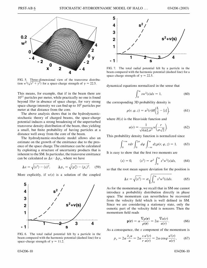
The overall effect of the space charge in this model is aconspicuous spreading of the transverse distribution ofthe particles in the beam with respect to the unperturbedground state distribution (52). When � � 0 the potentialdue to space charge vanishes, and the solution exactlycoincides with the ground state of the cylindrical har-monic oscillator with variance -2.When � > 0 the trans-verse distribution begins to spread, as we show in Figs. 2and 3 for a value of the space-charge strength � � 11:2,and in Figs. 4 and 5 for a value of the space-chargestrength � � 22:5. Notice that when comparing distribu-tions, the true radial (dimensionless) density is sw2�s�and not just w2�s�. Recall that w�s� is a normalizedsolution of Eqs. (49) and (50). In Figs. 6 and 7 we showthe radial transverse form of the total potential, i.e.,external plus space charge given by the solution v�s� ofEqs. (49) and (50), for the values � � 11:2 and � � 22:5

1 2 3 4- 0.2

0.2

0.4

0.6

0.8

s

s w2(s)

FIG. 2. The radial distribution sw2�s� compared withthe distribution in absence of space charge (dashed line).The space-charge strength is � � 11:2. All quantities aredimensionless.

034206-9

of the space-charge strength. To give a more quantitativemeasure of the flattening and broadening of the transversedistribution we compare numerically the probabilities offinding a particle at a relatively large distance from thebeam longitudinal axis with and without space charge.The quantity

P��c� �Z 1

c=��2

p sw2�s�ds (57)

is the probability of finding a particle at a distance greaterthan c- for systems with a given strength � of the space-charge coupling. For instance, considering the twodifferent situations � � 0 (no space charge) and � �22:5 (strong space charge) we have

P0�10� � 1:9� 10�22; P22:5�10� � 1:7� 10�6:

(58)

We see that the probability of finding particles at a dis-tance larger than 10- from the core of the beam isenhanced by space charge by many orders of magnitude.

1 2 3 4- 0.2

0.2

0.4

0.6

0.8

s

s w2(s)

FIG. 4. The radial distribution sw2�s� compared withthe distribution in absence of space charge (dashed line).The space-charge strength is � � 22:5. All quantities aredimensionless.

034206-9

- 4- 2

02

4x - 4

- 20

24

y0

0.2w2

- 4- 2

02x

FIG. 5. Three-dimensional view of the transverse distribu-tion w2�

��x2 � y2

p� for a space-charge strength of � � 22:5.

1 2 3 4- 1

1

2

3

4

5

s

s2+v(s)

s2

FIG. 7. The total radial potential felt by a particle in thebeam compared with the harmonic potential (dashed line) for aspace-charge strength of � � 22:5.


This means, for example, that if in the beam there are1011 particles per meter, while practically no one is foundbeyond 10- in absence of space charge, for very strongspace-charge intensity we can find up to 105 particles permeter at that distance from the core.

The above analysis shows that in the hydrodynamic-stochastic theory of charged beams, the space-chargepotential induces a strong broadening of the unperturbedtransverse density distribution of the beam, thus yieldinga small, but finite probability of having particles at adistance well away from the core of the beam.

The hydrodynamic-stochastic model allows also anestimate on the growth of the emittance due to the pres-ence of the space charge. The emittance can be calculatedby exploiting a structure of uncertainty products that isinherent to the SM. In particular, the transverse emittancecan be calculated as x �px, where we have

x ��hx2i � hxi2

q; px �

��hp2xi � hpxi

2q

: (59)

More explicitly, if w�s� is a solution of the coupled

1 2 3 4- 1

1

2

3

4

5

s

s2+v(s)

s2

FIG. 6. The total radial potential felt by a particle in thebeam compared with the harmonic potential (dashed line) for aspace-charge strength of � � 11:2.

034206-10

dynamical equations normalized in the sense thatZ 1

0sw2�s�ds � 1; (60)

the corresponding 3D probability density is

��r; ’; z� � u2�r�H�L2� jzj

�; (61)

where H�s� is the Heaviside function and

u�r� �1��

4'L-2p w

�r

-��2

p

�: (62)

This probability density function is normalized sinceZ �1

0rdr

Z 2'

0d’

Z 1

�1dz��r; ’; z� � 1: (63)

It is easy to show that the first two moments are

hxi � 0; hx2i � -2Z 1

0s3w2�s�ds; (64)

so that the root mean square deviation for the position is

x ��hx2i

q� -

��Z 1

0s3w2�s�ds

s: (65)

As for the momentum p, we recall that in SM one cannotintroduce a probability distribution directly in phasespace. The momentum can nevertheless be recoveredfrom the velocity field which is well defined in SM.Since we are considering a stationary state, only theosmotic part of the velocity field is nonzero. Then themomentum field reads

p�r� � r��r��r�

� 2ru�r�u�r�

: (66)

As a consequence, the x component of the momentum is

px � 2@xuu

� 2xru0�r�u�r�

� 2 cos’u0�r�u�r�

; (67)

034206-10

5 10 15 200.95

1.05

1.1

1.15

1.2

ε

γ

FIG. 8. The transverse dimensionless emittance " vs thespace-charge strength �. The true dimensional emittance,calculated as a position-momentum uncertainty product, isjust E � ".


and the first and second moments read

hpxi � 0; hp2xi �2

-2

Z 1

0w02�s�sds: (68)

Hence the root mean square deviation for the momentumis

px ��hp2xi

q�-

��Z 1

0w02�s�sds

s: (69)

We can then define the emittance E as the position-momentum uncertainty product in phase space in thefollowing way:

E � x �px �

��Z 1

0s3w2�s�ds �

Z 1

0w02�s�sds

s:

(70)

The emittance (70) can be thus estimated from knowl-edge of the numerical solutions w�s� and their first de-rivatives w0�s�. It can be seen that the emittance is exactly for � � 0 (namely, in absence of space charge), andgrows with � to a value � 1:2� for � � 22:5. Thisresult is consistent with the expected growth of emittanceproduced by space-charge effects. The dimensionless ra-tio " � E= � x �px= is plotted as a function of �in Fig. 8. This figure and the above discussion provideevidence that in the model of SM of charged beams theconstant plays the role of a lower bound for the phase-space emittance.

V. STATIONARY HALO DISTRIBUTIONS

The coupled nonlinear equations introduced in theprevious Section allow us to introduce and explain apossible mechanism of halo formation due to space-charge effects. This mechanism, when considering solu-tions without nodes, amounts to the broadening of thetransverse density distribution of the beam away from the

034206-11

beam core. This is a type of ‘‘continuous’’ halo. If wewant to investigate the formation and the properties ofother possible forms of halos—for example, ringlikehalos separated from the core by an almost void spaceregion—we should try to analyze the solutions withnodes of our radial self-consistent equations. This beinga time consuming task, we resort for the time being to adifferent, simplified approach to study the structure andproperties of beams of the ringed type.

Moreover, the scheme introduced in the previousSection, although in principle very general, has the draw-back that it does not allow for analytical expressions ofvelocities and potentials, and therefore cannot suggest theengineering of controlling external potentials to removethe halo. To this end, in this Section we will develop adifferent approach, still based on SM, by consideringsome preassigned density distributions for a beam withhalo and then looking for the kind of dynamics thatproduces them.

First of all we will determine the analytical forms ~ww�s�of the dimensionless radial distribution that can bestapproximate the numerical, self-consistent solutionsw�s� found in the previous Section. We will do that bychoosing a family of trial functions ~ww�s� and by subse-quently minimizing the mean square error with respectto a given solutionw�s�. Since the radial component of thecylindrically symmetric (l � 0) solutions of the har-monic oscillator (B1) contain only even powers of theradial coordinate (see Appendix B), we take as normal-ized trial functions

~ww�s� �e�s

2=2-2��c

p �1� as2 � bs4�; (71)

with -, a, and b as free parameters, and

c �Z 1

0e�s

2=-2�1� as2 � bs4�2sds

�-2

2� a-4 � �a2 � 2b�-6 � 6ab-8 � 12b2-10

(72)

as a normalization constant. We then take one numericalsolution w�s� of (49) and (50) for a given value of � andconsider the mean square error

J �Z 1

0jw�s� � ~ww�s�j2sds; (73)

and numerically minimize its value by varying the pa-rameters-, a, and b. As an example, for � � 19:3, we get

- � 1:81; a � 0:28; b � 0:01; c � 5:09:

(74)

The corresponding density distribution (solid line) iscompared in Fig. 9 with the density distribution obtainedby numerically solving the system (49) and (50) (dashedline). From this explicit form of the approximating ~ww�s�

034206-11

1 2 3 4 5 6 7

0.1

0.2

0.3

0.4

s

s w2(s)∼

FIG. 9. The best approximation in mean square (solid line) ofa numerical solution for the self-consistent equations (dashedline) for trial functions of the form (71) with � � 19:3.

1 2 3 4 5-1

1

2

3

4

5

s

v(s)s2+v(s)

∼

FIG. 10. The control potential (solid line) obtained from thebest mean square approximation ~ww�s� to a numerical solutionfor the self-consistent equations (49) and (50), for trial func-tions of the form (71) with � � 19:3. It is compared with thepotential s2 � v�s� (dashed line) obtained as a numericalsolution of (49) and (50).

5.5 6 6.5 7

0.0001

0.0002

0.0003

0.0004

s

s w2 (s)

s w2 (s)

∼

FIG. 11. Blown up picture of Fig. 9 that shows the existence ofa node in the position density distribution at s � 5:4.


we can now also calculate the expression of the stationarypotential which controls the state. From Eq. (37) in thecase of a cylindrically symmetric approximating statewith

~uu�r� ��~��r�

q; (75)

we have the controlling potential

~VV �r� � ~EE �2

2m

�~uu00�r�~uu�r�

�1

r

~uu0�r�~uu�r�

�: (76)

Introducing the usual dimensionless quantities

s �r

-��2

p ; ~�� 4m-2

2~EE; ~ww�s� � -3=2~uu�r�;

(77)

we may define the dimensionless controlling potential

~vv�s� � ~vv�r

-��2

p

��4m-2

2~VV �r� � ~��

~ww00�s�~ww�s�

�1

s~ww0�s�~ww�s�

:

(78)

For an approximating amplitude of the form (71), andwith the same values (74) of the parameters, the control-ling potential reads

~vv�s� �0:442� 0:629s2 � 0:062s4 � 0:001s6

1� 0:284s2 � 0:011s4: (79)

This potential is shown (solid line) in Fig. 10, where it iscompared with the potential s2 � v�s� (dashed line) sol-ution of Eqs. (49) and (50).

The analytical approximations show a small, but rele-vant, difference with respect to the numerical solutions ofEqs. (49) and (50): ~ww�s� has a node at about s � 5:4, andcorrespondingly the potential ~vv�s� has a singularity atthat point (out of the s range of Fig. 10). Instead, thenumerical solutions w�s� and v�s� of Eqs. (49) and (50)show no such behavior. For values of s beyond s � 5:4,~ww�s� shows a small bump, not visible in Fig. 9 because ofthe large scale. We show a zoom up of it in Fig. 11, where

034206-12

the node is now clearly visible. This is a feature that wewill find as well in other different approaches to thedescription of the beam distribution and that could betentatively connected with the presence of a halo spatiallyseparated from the core of the beam.

In our quest for an analytic description of the halodistribution we now depart from the scheme of the self-consistent nonlinear equations (49) and (50). Instead,while still assuming the space charge as the dominantfactor, we introduce a simplified analytical model for thehalo production. As a first simplification, valid for smallvalues of the space-charge strength �, we assume a frozencore for the beam. A frozen core is such that it produces aspace-charge effect, induces a spreading of the densitydistribution, and is left unchanged by this spreading. Inthis case the potential produced by the charge distributionis a priori given by the distribution of the frozen core andit simply enters linearly in the phenomenologicalSchrodinger equation (16). As a consequence, the latteris now decoupled from the Maxwell equations for theelectromagnetic field. The frozen charge distribution willbe assumed cylindrically symmetric and transversally

034206-12

1 2 3 4- 2

2

4

6

8

s

v (s)

FIG. 12. The dimensionless space-charge potential v�s� pro-duced by a frozen, cylindrically symmetric beam distributionwith � � 3.


Gaussian:

Q�r� � Nq0e��x2�y2�=2-2

2'-2

1

LH�L2� jzj

�; (80)

where N is the number of particles with elementarycharge q0, L is the longitudinal extension of the beam,and H�� denotes the Heaviside function. The cylindricalsymmetry allows one to determine via Gauss theorem thepotential energy Vsc�r� of a test particle of charge q0embedded in this charge distribution. It is a simple ex-ercise to show that

Vsc�r� �Nq202'(0L

�Ei

��

r2

2-2

�� ln

r2

2-2 � C

�; (81)

where C � 0:577 is the Euler constant, and

Ei�x� �Z x

�1

et

tdt (82)

is the exponential-integral function. If we suppose thatthe test particle is acted upon by this space-charge po-tential, and by the external, cylindrical harmonic oscil-lator potential (B1) —which, without space charge, wouldkeep the particle in the Gaussian state with variance-2 —the total potential to be inserted in the Schrodingerequation (16) reads

V�r� �2

8m-4 r2 �

Nq202'(0L

�Ei

��

r2

2-2

�� ln

r2

2-2 � C

�:

(83)

In terms of the usual dimensionless quantities we can alsowrite

s �r

-��2

p ; � �4m-2

2Nq202'(0L

;

v�s� � v�r

-��2

p

��4m-2

2V�r�

� s2 � � Ei��s2� � lns2 � C�:

(84)

A plot of the dimensionless potential v�s� for � � 3 isshown in Fig. 12.

For stationary solutions of the form

�r; t� � u�r�e�iEt=; (85)

Eq. (16) becomes

Eu�r� � HHu�r� � �2

2mr2u�r� � V�r�u�r�; (86)

and due to the cylindrical symmetry of V it reduces to

Eu�r� � �2

2m

�u00�r� �

u0�r�r

��V�r�u�r�: (87)

Considering the dimensionless quantities

034206-13

� �4m-2

2E; w�s� � w

�r

-��2

p

�� -3=2u�r�; (88)

we finally obtain the reduced equation

�w�s� � �w00�s� �w0�s�s

� v�s�w�s�: (89)

Despite its simple graphical behavior displayed in Fig. 12the potential v�s� is complicated enough to bar the hopeof exactly solving Eq. (89) in a simple way. Reasonableapproximate solutions can be obtained by means of thevariational method of Rayleigh and Ritz.We thus look forthe minimum of the average energy

�u; HHu��u; u�

; (90)

whose reduced and dimensionless form isR10 �w�s�w

00�s�s� w�s�w0�s� � v�s�w2�s�s�dsR10 w

2�s�sds: (91)

The minimization can be carried out for different valuesof the coupling parameter �, but the frozen core modelis realistic only for small values of �: a strong couplingwith a frozen core would have the paradoxical effect oftotally expelling the distribution function of the testparticle from the center of the beam, while keeping theGaussian core always concentrated in the center. To elab-orate an example we have chosen � � 3 and a test func-tion of the form

w�s� �e�s

2=2-2��c

p �1� as2 � bs4�: (92)

The values of the parameters that minimize the energyfunctional turn out to be

- � 1:24; a � 0:63; b � 0:03; c � 2:92:

(93)

The corresponding optimal radial density distribution

034206-13

FIG. 13. The variational approximation to the density distri-bution produced by the space charge of a frozen core with � �3 (solid line). It is compared with the Gaussian solution (dashedline) corresponding to the case of a purely harmonic potential(� � 0).


sww2�s� is shown in Fig. 13 where it is also compared withthe Gaussian solution (dashed line) corresponding to thecase of a purely harmonic potential (� � 0). Notice thatthis density distribution has a form similar to that of theself-consistent solutions elaborated in Sec. IV for valuesof � of about 10 (see Fig. 2). It has a node which is notvisible in Fig. 13. We zoom up its plot in Fig. 14. Thisbehavior suggests that the halo distribution could bedescribed, in first approximation, as a Gaussian core dis-tribution plus a small ring of particles surrounding it andconstituting the halo. Thus, in the following we willsimply assume a specific form of a beam with a halowithout deriving it as an effect of space-charge interac-tions. Since it is not clearly established that a halo can bedue only to space-charge effects, starting with a realisticring distribution and trying to understand the dynamicsthat can produce it could be very useful in this respect.The techniques introduced in Sec. III will be instrumen-tal to this end. For a three-dimensional, cylindricallysymmetric beam we introduce the normalized radialdensity distribution

��r� � Ae�r

2=2-2

-2 � �1� A�e�r

2=2p2-2

p2-2 �q� 1�

�r2

2p2-2

�q

(94)

FIG. 14. Zoom up of Fig. 13 that shows a node in the positiondensity distribution at s � 4:7.

034206-14

which is composed of a Gaussian core with variance -2

(the simple harmonic oscillator ground state), plus a ring-like distribution whose size is fixed through the twoparameters p > 0 and q � 0. The parameter 0 � A � 1is the relative weight of the two parts. This density dis-tribution has the required form for suitable values of theparameters, but, at variance with the two previous exam-ples of approximate distributions (see Figs. 11 and 14), ithas no nodes. This is convenient for two main reasons:first because it is a rather general requirement for a groundstate to have no nodes (this fact is a rigorous theorem forone-dimensional systems). Moreover, it has been shownin Refs. [30,32,33] that stationary distributions withoutnodes are also attractors for every other possible (nonex-tremal) initial distribution: a property that will be usefulin a future discussion of the possible relaxation of thesystem toward a stable beam halo. For this cylindricallysymmetric case the expressions (30) and (37) for thevelocity field and the potential become

u�r� ��r�

q;

v��r� �mu0�r�u�r�

;

V�r� �2

2m-2 �2

2m

�u00�r�u�r�

�1

ru0�r�u�r�

�: (95)

Moving to dimensionless quantities we have

s �r

-��2

p ;

w2�s� � w2

�r

-��2

p

�� 2-2��r�

� 2Ae�s2� 2�1� A�

e�s2=p2

p2 �q� 1�

�s2

p2

�q;

b�s� � b�r

-��2

p

��m-

��2

p

v��r� �

w0�s�w�s�

;

v�s� � v�r

-��2

p

��4m-2

2V�r� � 2�

w00�s�w�s�

�1

sw0�s�w�s�

:

(96)

A three-dimensional plot of the dimensionless densitydistribution is given in Fig. 15 where we have chosen p �1, q � 24, and A � 0:49. In this example the importanceof the halo ring has been exaggerated with respect to thereal case in order to make the effect clearly visible. Theexplicit analytic expression of b�s� and v�s� is ratherlengthy and not particularly illuminating: we simplyshow the behavior of these functions, for the same valuesof the parameter for the previous example, respectively,in Figs. 16 and 17, where they are also compared with the

034206-14

- 50

5x - 5

0

5

y0

0.8w2

- 50

5x

FIG. 15. Plot of the cylindrically symmetric density distri-bution of the beam w2�

��x2 � y2

p� given by Eq. (96), which

shows a halo ring surrounding the beam core.

1 2 3 4 5 6 7- 10

10

20

30

40

50

s

s2

v (s)

FIG. 17. The radial, dimensionless, potential for the distri-bution of Fig. 15 (solid line), and for a harmonic oscillator(dashed line).


corresponding dimensionless quantities ( � s and s2) forthe ground state of the harmonic oscillator. The functionv�s� is the potential that in the stochastic model keeps thebeam in the stationary state with a halo ring.

In order to illustrate the main effects involved, let usgive here the simpler formulas relative to the 1D case.From now on we will consider only 1D processes denotingby x one of the transverse space coordinates. We assumethat the longitudinal and the transverse beam dynamicscan be deemed independent, with the further simplifica-tion of considering decoupled evolutions along the trans-verse directions x and y. Under these conditions thedensity distribution with a halo ring now reads

��x� � Ae�x

2=2-2

-��2'

p � �1� A�e�x

2=2p2-2

p-��2

p �q� 1

2�

�x2

2p2-2

�q;

(97)

so that the corresponding velocities and potential are

1 2 3 4 5 6 7

- 6

- 4

- 2

2

s

- s

b (s)

FIG. 16. The radial, dimensionless, forward velocity field forthe distribution of Fig. 15 (solid line), and for the ground stateof a harmonic oscillator (dashed line).

034206-15

u�x� ��x�

q;

v��x� �mu0�x�u�x�

;

V�x� �2

4m-2 �2

2mu00�x�u�x�

: (98)

In terms of dimensionless quantities we then have for thedistribution

s �x

-��2

p ;

w2�s� � w2

�x

-��2

p

�� 2-2��x�

� Ae�s

2��'

p � �1� A�e�s

2=p2

p �q� 12�

�s2

p2

�q; (99)

while the forward velocity and the potential are

b�s� � b�x

-��2

p

��m-

��2

p

v��x� �

w0�s�w�s�

; (100)

- 6 - 4 - 2 2 4 6

0.1

0.2

0.3

0.4

s

FIG. 18. Plot of the 1D density distribution (97) with a haloring surrounding the beam core.

034206-15

- 6 - 4 - 2 2 4 6

- 6

- 4

- 2

2

4

6

s

- s

b (s)

FIG. 19. The dimensionless velocity for the 1D distribution ofFig. 18 (solid line), and for a harmonic oscillator (dashed line).

- 6 - 4 - 2 2 4 6

10

20

30

40

50

s

s2

v (s)

FIG. 20. The dimensionless potential for the 1D distributionof Fig. 18 (solid line), and for a harmonic oscillator (dashedline).


v�s� � v�x

-��2

p

��4m-2

2V�x� � 1�

w00�s�w�s�

: (101)

In Figs. 18–20, we, respectively, show the density distri-bution, the velocity field, and the potential for p � 1, q �24, and A � 0:85. As in the three-dimensional case, theimportance of the halo ring has been exaggerated withrespect to the real case in order to make the effect clearlyvisible.

VI. CONCLUSIONS

In this paper we have presented a dynamical, stochasticapproach to the description of the beam transverse dis-tribution in the particle accelerators. In the first part wehave described the collective beam dynamics in terms oftime-reversal invariant diffusion processes (Nelson proc-esses) which are obtained by a stochastic extension of theleast action principle of classical mechanics. The diffu-sion coefficient of the process is identified with a lowerbound for the emittance of the beam as discussed inSec. IV. The collective dynamics of beams is then de-

034206-16

scribed by two nonlinearly coupled hydrodynamic equa-tions. This set of equations shows some formal analogieswith the effective Ginzburg-Landau and Gross-Pitaevskiidescriptions of the collective dynamics of self-interactingquantum many-body systems in terms of a classical, non-linear Schrodinger equation. We have shown that, in theframework of SM, it is possible to have transverse dis-tribution which shows a broadening and an emittancegrowth, typical of the halo formation. The interest ofthis approach lies in the fact that its dynamical equationsallow us, at least in principle, to determine the possiblecontrol potentials that are responsible for the stationarityof the halo. A few introductory examples of these poten-tials and distributions have been discussed in Sec. V. Thecontrolling potentials can be engineered by suitable tun-ing of the external electromagnetic fields. In a previouspaper [20] we have considered evolutions that drive thebeam from a less collimated to a better collimated state,and we have furthermore shown that this goal can also beachieved without increasing the frequency of the betatronoscillations which can in fact be independently controlledduring the evolution. In forthcoming papers we plan toelaborate on the extension of these techniques to theproblem of engineering suitable time-dependent poten-tials for the control and the elimination of the beam halo.In particular, it will be shown that the transition func-tions of the Nelson processes can be exploited to controlthese evolutions.We also plan to extend the analysis of thepresent paper to different, non-Gaussian beam transversedistributions which could better describe the existence ofhalo losses in terms of large ratios of the maximumdisplacement to the rms size of the beam.

ACKNOWLEDGMENTS

We thank Armando Bazzani, Oliver Boine-Frankenheim, Francesco Guerra, Ingo Hofmann, andGiorgio Turchetti for many valuable discussions alongthe writing of this paper. We also acknowledge thefinancial support from INFN–Istituto Nazionale diFisica Nucleare (experiment MQSA), INFM–IstitutoNazionale per la Fisica della Materia, and MIUR–Ministero dell’Istruzione, dell’Universita e dellaRicerca. Two of us (S. D. M. and S. D. S.) acknowledgesupport of the ESF COSLAB program.

APPENDIX A: COUPLED FIELD EQUATIONS

Starting from the Maxwell equations for the space-charge field felt by our particle in the beam

r � Esc�r; t� ��sc�r; t�(0

;

r� Esc�r; t� � �@tBsc�r; t�;

r � Bsc�r; t� � 0;

034206-16


r�Bsc�r; t� � 50jsc�r; t� �@tEsc�r; t�

c2;

and introducing the corresponding electromagnetic po-tentials �Asc;�sc� from

Bsc�r; t� � r�Asc�r; t�;

Esc�r; t� � �@tAsc�r; t� � r�sc�r; t�;

with the gauge condition

r �Asc�r; t� �1

c2@t�sc�r; t� � 0; (A1)

through the usual procedure we get the wave equations

r2Asc�r; t� �1

c2@2tAsc�r; t� � �50jsc�r; t�; (A2)

r2�sc�r; t� �1

c2@2t�sc�r; t� � �

�sc�r; t�(0

: (A3)

It is also well known (see, for example, [16], chapter XV)that the Schrodinger equation for spinless, charged par-ticles in an electromagnetic field �A;�� is

i@t �

�1

2m

�ir�

q0cA�2�q0�

� :

For a charged particle in the beam the electromagneticfield is the superposition of the space-charge potential�Asc;�sc� plus an external, control potential �Aext;�ext�,and hence we obtain the Schrodinger equation (43) thatwe rewrite here for convenience:

i@t �1

2m

�ir�

q0c�Asc �Aext�

�2

� q0��sc ��ext� : (A4)

It is apparent now that (A1)–(A4) constitute a self-consistent system of coupled, nonlinear differential equa-tions for the fields , Asc, and �sc.

Since we are in a reference frame comoving with thebeam, in the following we will deal only with stationarywave functions of the form (42). In this case, as alreadyremarked, we get jsc � 0, so that we can take the trivialsolution Asc � 0 of (A2). The gauge condition (A1) thenimplies that @t�sc � 0 and the wave equation (A3) re-duces itself to the Poisson equation for the electrostaticpotential. Finally, by supposing also Aext � 0, our systemis reduced to only two coupled, nonlinear equations forthe couple �u;�sc�, namely,

Eu � �2

2mr2u� q0��ext ��sc�u;

r2�sc � �Nq0(0

juj2

ku2k;

034206-17

where we have defined

ku2k �ZR3

ju�r; t�j2d3r:

Then if we pass to the potential energies by putting

Vext�r; t� � q0�ext�r; t�; Vsc�r; t� � q0�sc�r; t�;

our equations are reduced to

2

2mr2u� �E� Vext � Vsc�u � 0; (A5)

r2Vsc � �Nq20(0

juj2

ku2k: (A6)

We remark that here the wave functions and u, whilecertainly normalizable, are not supposed in general tobe already normalized. However the equations (A5) and(A6), albeit nonlinear, are apparently invariant for themultiplication of u by an arbitrary constant. Theequations (A5) and (A6) will be used in Sec. IV.

APPENDIX B: CYLINDRICAL HARMONICOSCILLATOR

In the model discussed in this paper we suppose thatthe external potential Ve is a cylindrically symmetric,harmonic potential with a proper frequency!, so that theground state without space-charge interaction will have avariance

-2 �

2m!:

This means that, in the usual cylindrical coordinatesfr; ’; zg with r �

��x2 � y2

p, we have

Ve�r� �m2!2r2 �

2

8m-4 r2; (B1)

and the corresponding Schrodinger equation

i@t � �2

2mr2 � Ve

� �2

2m

�1

r@r�r@r� �

1

r2@2’ � @2z

� � Ve

with periodic conditions at z � �L=2 (for a bunch oflength L) has the eigenvalues

Enk � �n� 1�!� k2�2'-L

�2!

and the normalized eigenfunctions

nkl�r; ’; z; t� � Rnl�r��l�’�Zk�z�e�iEnkt=

with

Rnl�r� �

��n�l2 �!

�n�l2 �!

vuut e�r2=4-2

-

�r

-��2

p

�lL�l��n�l=2�

�r2

2-2

�;

034206-17


�l�’� �eil’��2'

p ;

Zk�z� �ei2k'z=L��

Lp ;

where L�q�p �x� are the generalized Laguerre polynomials

and

n � 0; 1; 2; . . . ;

l ��0; 2; 4; . . . ; n if n even;1; 3; 5; . . . ; n if n odd;

k � 0;�1;�2; . . . :

We suppose that, by neglecting the space-charge interac-tion and in a comoving frame of reference, the systemwill be correctly described by the ground state

000�r� �e�r

2=4-2

-��2'L

p (B2)

associated to the eigenvalue E00 � !.

03420

[1] H. Koziol, Los Alamos M. P. Division Report No. MP-3-75-1, 1975.

[2] M. Reiser, C. Chang, D. Kehne, K. Low, T. Shea, H. Rudd,and J. Haber, Phys. Rev. Lett. 61, 2933 (1988).

[3] R. L. Gluckstern, Phys. Rev. Lett. 73, 1247 (1994).[4] R. L. Gluckstern,W.-H. Cheng, and H. Ye, Phys. Rev. Lett.

75, 2835 (1995).[5] R. L. Gluckstern,W.-H. Cheng, S. S. Kurennoy, and H. Ye,

Phys. Rev. E 54, 6788 (1996).[6] H. Okamoto and M. Ikegami, Phys. Rev. E 55, 4694

(1997).[7] R. L. Gluckstern, A.V. Fedotov, S. S. Kurennoy, and

R. Ryne, Phys. Rev. E 58, 4977 (1998).[8] T. P. Wangler, K. R. Crandall, R. Ryne, and T. S. Wang,

Phys. Rev. ST Accel. Beams 1, 084201 (1998).[9] A.V. Fedotov, R. L. Gluckstern, S. S. Kurennoy, and

R. Ryne, Phys. Rev. ST Accel. Beams 2, 014201 (1999).[10] M. Ikegami, S. Machida, and T. Uesugi, Phys. Rev. ST

Accel. Beams 2, 124201 (1999).[11] J. Quiang and R. Ryne, Phys. Rev. ST Accel. Beams 3,

064201 (2000).[12] O. Boine-Frankenheim and I. Hofmann, Phys. Rev. ST

Accel. Beams 3, 104202 (2000).

6-18

[13] L. Bongini, A. Bazzani, G. Turchetti, and I. Hofmann,Phys. Rev. ST Accel. Beams 4, 114201 (2001).

[14] A.V. Fedotov and I. Hofmann, Phys. Rev. ST Accel.Beams 5, 024202 (2002).

[15] T. Wangler, RF Linear Accelerators (Wiley, New York,1998).

[16] L. D. Landau and E. M. Lifshitz, Physical Kinetics(Butterworth-Heinemann, Oxford, 1996).

[17] F. Ruggiero, Ann. Phys. (N.Y.) 153, 122 (1984);F. Ruggiero, E. Picasso, and L. A. Radicati, Ann. Phys.(N.Y.) 197, 396 (1990).

[18] J. Struckmeier, Phys. Rev. ST Accel. Beams 3, 034202(2000).

[19] W. Paul and J. Baschnagel, Stochastic Processes: FromPhysics to Finance (Springer, Berlin, 2000).

[20] N. Cufaro Petroni, S. De Martino, S. De Siena, andF. Illuminati, Phys. Rev. E 63, 016501 (2001); inQuantum Aspects of Beam Physics 2K, edited by P.Chen (World Scientific, Singapore, 2002), p. 507.

[21] S. De Martino, S. De Siena, and F. Illuminati, Physica(Amsterdam) 271A, 324 (1999).

[22] E. Nelson, Dynamical Theories of Brownian Motion(Princeton University Press, Princeton, NJ, 1967);Quantum Fluctuations (Princeton University Press,Princeton, NJ, 1985).

[23] F. Guerra, Phys. Rep. 77, 263 (1981).[24] F. Guerra and L. M. Morato, Phys. Rev. D 27, 1774

(1983).[25] S. Albeverio, Ph. Blanchard, and R. Høgh-Krohn, Expo.

Math. 4, 365 (1983).[26] R. Fedele, G. Miele, and L. Palumbo, Phys. Lett. A 194,

113 (1994), and references therein; S. I. Tzenov, Phys.Lett. A 232, 260 (1997).

[27] S. A. Khan and M. Pusterla, Eur. Phys. J. A 7, 583 (2000).[28] L. Morato, J. Math. Phys. (N.Y.) 23, 1020 (1982).[29] E. Madelung, Z. Phys. 40, 332 (1926); D. Bohm, Phys.

Rev. 85, 166 (1952); 85, 180 (1952).[30] N. Cufaro Petroni, S. De Martino, S. De Siena, and

F. Illuminati, J. Phys. A 32, 7489 (1999).[31] N. Cufaro Petroni, S. De Martino, S. De Siena, and

F. Illuminati, in Quantum Aspects of Beam Physics,edited by P. Chen (World Scientific, Singapore, 1999),p. 710; N. Cufaro Petroni, S. De Martino, S. De Siena,R. Fedele, F. Illuminati, and S. I. Tzenov, in Proceedingsof the European Particle Accelerator Conference —EPAC98, Stockholm, Sweden, edited by S. Myers et al.(IOP Publishing, Bristol, 1998), p. 1259.

[32] N. Cufaro Petroni and F. Guerra, Found. Phys. 25, 297(1995).

[33] N. Cufaro Petroni, S. De Martino, and S. De Siena, Phys.Lett. A 245, 1 (1998).

034206-18

stochastic-hydrodynamic model of halo formation in charged ...cufaro/scientific/2003_pr-stab.pdf ·...

Documents