phase portrait approximation using dynamic neural networks

Phase portrait approximation using dynamic neural networks

Alberto Delgado*

Electrical Engineering Department, National University of Colombia, A.A. No. 5885, Bogota, DC 103092, USA

Received 25 November 1997; accepted 1 December 1997

Abstract

In this paper it is shown that a nonlinear system with an isolated equilibrium can be identified using two kinds of Dynamic

Neural Networks, the Hopfield type (DNN-H) and the Multilayer type (DNN-M). The identified models are in continuous

time. The equilibrium point is assumed to be the origin, without loss of generality, and it is assumed to be stable. Two different

approaches are used to identify the nonlinear system, the first one is a phase portrait identification and the second one is the

identification of the input/output response. The phase portraits for the two models are plotted and the eigenvalues of the

Jacobian of the plant and the Jacobian of the models are calculated to make comparisons. Both networks can be used to

identify nonlinear systems. The DNN Multilayer type is used to keep the number of states at a minimum, i.e., the number of

states of the network is the same as the plant, the approximation capabilities of the DNN-M are increased by increasing the

number of neurons of the internal multilayer network keeping the number of states constant. The DNN Hopfield type is used

to obtain a state representation without hidden units but the number of states is not minimum, that is, the DNN-H equations are

simpler but the number of states may be higher than the number of states of the plant. # 1998 Published by IMACS/Elsevier

Science B.V.

Keywords: Dynamic neural networks; Identification; Input/output response; Nonlinear systems; Phase portrait

1. Introduction

It has been shown extensively that Neural Networks can approximate nonlinear mappings to anydegree of accuracy [3,8]. This approximation of nonlinear maps is achieved with multilayer neuralnetworks, the accuracy is increased by manipulating the number of hidden layers and the number ofhidden neurons.

Neural Networks can be used, also, to approximate dynamic systems in continuous time. In this casethere are two types of networks: the Dynamic Neural Network hopfield type (DNN-H) and theDynamic Neural Network Multilayer type (DNN-M). Funahashi and Nakamura [9] proved thatdynamic networks of the Hopfield type can approximate dynamic systems to any degree of accuracy. In

Mathematics and Computers in Simulation 47 (1998) 1±11

ÐÐÐÐ

* E-mail: [email protected]

0378-4754/98/$19.00 # 1998 Published by IMACS/Elsevier Science B.V. All rights reserved

PII S 0 3 7 8 - 4 7 5 4 ( 9 7 ) 0 0 1 6 1 - 4

the context of geometric control, Delgado et al. [4±6] and Kambhampati et al. [11] have used DNNs-Hto identify and control nonlinear affine systems.

On the other hand, one graphic tool to understand the behaviour of nonlinear differential equations isthe phase portrait, Jordan and Smith [10], Sanchez [12]. In this case the differential equations thatdescribe the system are known and the phase portrait of the system is plotted by using the vector field orvelocity field. Despite the phase portrait is an old technique to study linear/nonlinear differentialequations, the inverse problem has not been discussed yet. The inverse problem is as follows: given themeasured vector field or velocity field of an autonomous linear/nonlinear system find the differentialequations that describe the system.

In this paper a proposition that shows how a DNN-M can be used to approximate the phase portrait anonlinear systems is stated and proved, also it is shown how this DNN-M can be unfolded into a DNN-H and the DNN-H can be folded into a DNN-M. The mathematical procedures are illustrated withnumerical simulations.

2. Vector field approximation

A proposition that shows how the vector field of a nonlinear autonomous system can beapproximated by the vector field of a Dynamic Neural Network ± Multilayer type (DNN-M) is statedand proved.

Proposition: Consider the nonlinear autonomous system

d

dtx � f �x� � A:x� f0�x� (1)

and the DNN-H

d

dtz � f �z� � A:z�W :��T :z� (2)

where x, z 2 Rn, A 2 Rn�n, f �x� : Rn ! Rn, f �z� : Rn ! Rn, W 2 Rn�N , T 2 RN�n,��z� � ��z1�; ��z2�; . . . ; ��zn��; ��:� � tanh�:�. Note that, without loss of generality, the origin isassumed to be the equilibrium point and the system (Eq. (1)) will be identified with the network (Eq.(2)) around its basin of attraction.

The approximation error e(t) is bounded:

ke�t�k � kx�t� ÿ z�t�k � M: ke�0�k � K� �:eÿm2:t (3)

with K, M and m positive constants, if the following conditions are satisfied

(i) k��t�k � keA:tk � M:eÿm:t, i.e., the matrix A is Hurwitz.(ii)R t

0em:� :k f0�x� ÿW :��T :x�k:d� � R t

0em:� :"1:d� � K where,

Maxx2D; D�Rn

k f0�x� ÿW :��T :x�k � "1;

that is, the function f0(x) is approximated by the function W.�(T.x) in the region of interest. The error"0 can be decreased arbitrarily changing the matrices W and T.

2 A. Delgado / Mathematics and Computers in Simulation 47 (1998) 1±11

(iii) kW :��T :x� ÿW :��T:z�k � l:kxÿ zk. The sigmoid function �(.) is Lipschitz with Lipschitzconstant l�m/2M.

Proof: The approximation error e(t) and its time derivative are,

e�t� � x�t� ÿ z�t�d

dte�t� � d

dtx�t� ÿ d

dtz�t�

Replacing the nonlinear system equation (Eq. (1)) and network equation (Eq. (2)) yields,

d

dte�t� � A:x� f0�x� ÿ A:zÿW :��T :z� � A:e�t� � f0�x� ÿW :��T :z�

this can be written as,

d

dte�t� � A:e�t� � � f0�x� ÿW :��T:x�� W :��T :x� � W :��T :z��

Solving this differential equation,

e�t� � ��t�:e�0� �Zt0

��t ÿ ��:� f0�x� ÿW :��T:x��:d�

�Zt0

��t ÿ ��:�W :��T :x� ÿW :��T:z��:d�

taking the norm,

ke�t�k � M:eÿm:tke�0�k �Zt0

M:eÿm:t:em:�k f0�x� ÿW :��T :x�k:d�

�Zt0

M:eÿm:t:em:� :kW :��T :x� ÿW:��T:z�k:d�

replacing the conditions (i), (ii), (iii) from the proposition,

ke�t� � M:eÿm:t: ke�0�k � K� � �Zt0

M:eÿm:t:em:� :l:ke��k:d�

moving the exponential to the left side, this equation can be written as,

ke�t�k:em:t � M: ke�0�k � K� � �Zt0

M:m

2M:ke��k:em:� :d�

and, applying the Gronwall±Bellman lemma [10,12] we get,

ke�t� � M: ke�0�k � K� �:eÿm2:t

&

A. Delgado / Mathematics and Computers in Simulation 47 (1998) 1±11 3

This proposition proves that the vector field of the autonomous system (Eq. (1)) can be approximatedby the vector field of a DNN-M (Eq. (2)) if the conditions (i), (ii) and (iii) are satisfied. Theapproximation error e(t) is bounded and decreases exponentially with time, note that the value of Kgoes to zero when the approximation of condition (ii) is improved.

3. Identification with a DNN-M

Consider the autonomous single link manipulator shown in Fig. 1. This system is described by thedifferential equations

dx1

dt� x2 (4)

dx2

dt� ÿ9:8sinx1 ÿ 0:5x2 � 0:5:u

y � x1

where x1 � �; x2 � d�=dt; u 2 R is the plant input, and y 2 R is the plant output. The Jacobian of theplant at the origin yields,

Jp � 0:0 1:0ÿ9:8 ÿ0:5

� �and the corresponding eigenvalues are: �1;2 � ÿ0:25� j3:12.

A DNN-M was trained to approximate the vector field of the autonomous �u � 0� single linkmanipulator over the operating region (a region of interest): x1; x2 2 �ÿ1:0; 1:0�: The block diagram ofthe network is shown in Fig. 2. The multilayer network used in this dynamic network has the structuren±N±n, i.e., n input nodes, N hidden neurons, and n output nodes.

In the simulation below n � 2; N � 2 and A � ÿIn (In is the identity matrix of dimension n).The goal of the training algorithm is to find the matrices W and T of model (Eq. (2)) to identify theplant (Eq. (4)). To train the network, 400 points (x1, x2) were generated randomly in the region

Fig. 1. Nonlinear control affine system: single link manipulator.


of interest, for each point the vector field of the plant was calculated. The network was trained withthe chemotaxis algorithm, Bremermann [1,2], to match the vector field of the plant, the performanceindex was,

J � 1

NS

XNS

k�1

� f1�xk1; x

k2� ÿ f

1�xk

1; xk2��2 � � f2�xk

1; xk2� ÿ f

2�xk

1; xk2��2

h i( )12

(5)

where NS is the number of points in the phase plane and fi�x�; f i�z�jz�x, are the components of the

vector fields of the plant and the network respectively. The training algorithm is used to minimise theindex J, at the end of a successful training the matrices W and T are found.

After training, the neural network (Eq. (2)) can be written as,

d

dt

z1

z2

� �� ÿ1:0 0:0

0:0 ÿ1:0

� �z1

z2

� �� ÿ3:2466 2:8860

9:7322 3:9356

� �� ÿ0:8142:z1 ÿ 0:0735:z2��ÿ0:4998:z1 � 0:3056:z2��

(6)

Figs. 3 and 4 show the phase portraits of the trained network (Eq. (6)) and the plant (Eq. (4))respectively, starting from the initial condition x1�0� � x2�0� � 0:8; z1�0� � z2�0� � 0:8.

The Jacobian of the DNN-M at the origin yields,

JM � ÿIn �W :T � 0:2009 1:1208

ÿ9:8909 ÿ0:5128

� �and the corresponding eigenvalues are: �1;2 � ÿ0:16� j3:31.

Comparing the phase portraits (Figs. 3 and 4) and comparing the eigenvalues, it is clearthat the network (Eq. (6)) has captured the dynamics of the nonlinear plant (Eq. (4)) in theregion of interest. The network (Eq. (4)) is slower than the plant, that is, starting from the sameinitial condition and with the same simulation time, the plant reaches the origin faster than thenetwork.

Fig. 2. Block diagram of a DNN-M (Eq. (2)). During the training the parameters W � !ij; T � tij are determined.


4. Transforming a DNN-M into a DNN-H

The Dynamic Neural Network Multilayer type (Eq. (2)) can be transformed into a Dynamic NeuralNetwork Hopfied type (DNN-H) using a linear transformation,

� � T :z (7)

d�

dt� T :

dz

dt

In our case T is a square matrix but it can be easily shown (with a generalized inverse) that thenetwork (Eq. (2)) with the transformation (Eq. (7)) and A � ÿIn; T 2 RN�n (a non-square

Fig. 3. Phase portrait of the single link manipulator (Eq. (4)) starting from the initial condition x1�0� � x2�0� � 0:8. The

simulation time was 20 s.

Fig. 4. Phase portrait of the trained DNN-M (Eq. (6)) starting from the initial condition z1�0� � z2�0� � 0:8: The simulation

time was 20 s.


transformation matrix) can be reduced to,

d

dt� � ÿIN :�� T:W :�� (8)

where the new state vector � 2 RN and T :W 2 RN�N , IN is the identity matrix of dimension N. Notethat a DNN-M has x 2 Rn and W:T 2 Rn�n.

It can be said that the transformation (Eq. (7)) unfolds the DNN-M (Eq. (2)) into the DNN-H (Eq.(8)). That is, there are no hidden units in the type H network but the number of states is greater or equalto the number of states in the type M network, N�n.

Transforming the DNN-M (Eq. (6)) into a DNN-H,

d

dt

�1

�2

� �� ÿ1:0 0:0

0:0 ÿ1:0

� �:�1

�2

� �� 1:9281 ÿ2:6390

4:5968 ÿ0:2397

� �:��1��2

� �(9)

The Jacobian of the DNN-H at the origin yields,

JH � ÿIN � T :W � 0:9281 ÿ2:6390

4:5968 ÿ1:2397

� �and the corresponding eigenvalues are: �1;2 � ÿ0:16� j3:31. The Fig. 5 shows the phase portrait ofnetwork (Eq. (9)) for the same initial conditions and simulation time as before, notice that thecoordinate transformation has changed the shape and direction of the phase trajectory but theeigenvalues are still the same.

5. Identification with a DNN-H

It is possible to identify directly the single link manipulator (Eq. (4)) using a DNN-H in theconfiguration of Fig. 6.

Fig. 5. Phase portrait of the DNN-H (Eq. (9)) starting from the initial condition �1�0� � �2�0� � 0:8: The simulation time

was 20 s.


In this case the DNN-H state equation is,

d

dt� � ÿIN :�� T:W :�� ÿ:u

yn � �1

The training of the DNN-H is carried out with the chemotaxis algorithm to reduce theperformance index (Eq. (10)) that is function of the identification error ei during a time interval�0; tf �;

Ji �

��1

tf

Ztf0

e2i �t�:dt

vuuut �

��1

tf

Ztf0

�y�t� ÿ yn�t��2:dt

vuuut (10)

After training, the identified autonomous DNN-H N�2 states is:

d

dt

�1

�2

� �� ÿ1:0 0:0

0:0 ÿ1:0

� �:�1

�2

� �� ÿ1:9542 ÿ4:0983

4:3264 3:5834

� �:��1��2��

(11)

with �(.)� tanh (.). Fig. 7 shows the phase trajectory of network (Eq. (11)) from the initial condition�1�0� � �2�0� � 0:8.

The Jacobian of the DNN-H at the origin yields,

JH � ÿ2:9542 ÿ4:0983

4:3264 2:5834

� �with eigenvalues �1;2 � ÿ0:18� j3:17.

Comparing the phase portraits (Figs. 3 and 7) and comparing the eigenvalues, it is clear that thenetwork (Eq. (11)) has captured the dynamics of the nonlinear plant (Eq. (4)) in the region of interest.The DNN-H is slower than the plant, that is, starting from the same initial condition and for the samesimulation time, the plant reaches the origin faster than the network. Notice that the direction and shape

Fig. 6. Identification of a single link manipulator using a DNN-H.


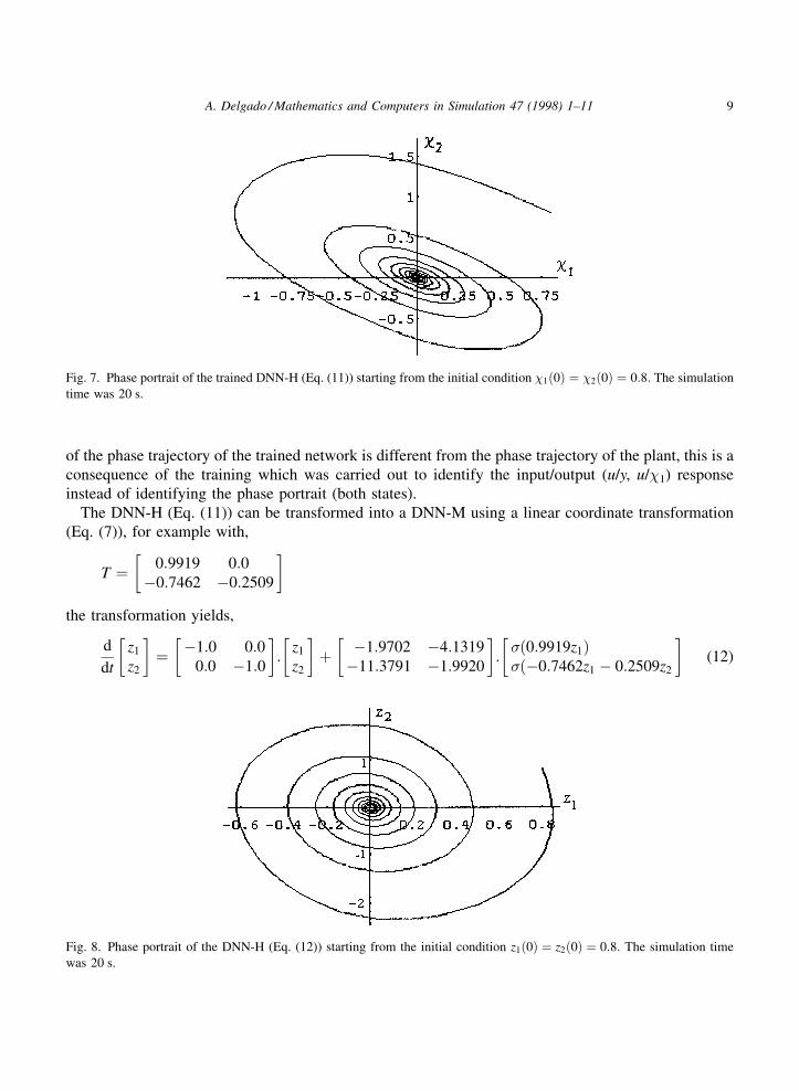
of the phase trajectory of the trained network is different from the phase trajectory of the plant, this is aconsequence of the training which was carried out to identify the input/output (u/y, u/�1) responseinstead of identifying the phase portrait (both states).

The DNN-H (Eq. (11)) can be transformed into a DNN-M using a linear coordinate transformation(Eq. (7)), for example with,

T � 0:9919 0:0ÿ0:7462 ÿ0:2509

� �the transformation yields,

d

dt

z1

z2

� �� ÿ1:0 0:0

0:0 ÿ1:0

� �:

z1

z2

� �� ÿ1:9702 ÿ4:1319

ÿ11:3791 ÿ1:9920

� �:��0:9919z1��ÿ0:7462z1 ÿ 0:2509z2

� �(12)

Fig. 7. Phase portrait of the trained DNN-H (Eq. (11)) starting from the initial condition �1�0� � �2�0� � 0:8: The simulation

time was 20 s.

Fig. 8. Phase portrait of the DNN-H (Eq. (12)) starting from the initial condition z1�0� � z2�0� � 0:8: The simulation time

was 20 s.


The Jacobian of the DNN-M at the origin yields,

JM � 0:1290 1:0367

ÿ9:8005 ÿ0:5002

� �and the corresponding eigenvalues are: �1;2 � ÿ0:18� j3:17: The Fig. 8 presents the phase portrait ofnetwork (Eq. (12)) for the same initial condition and simulation time as before. Notice, again, that thelinear transformation has changed the shape and direction of the phase trajectory but the eigenvaluesare preserved.

6. Conclusions

It was proved that a DNN-M can be used to approximate the phase portrait of nonlinear systems andto provide a set of first order differential equations, this is the solution of the inverse problem. In thisapproach the vector field of the network is adjusted to match the vector field of the system, that is, thevector field of the system is printed onto the network.

Using a linear transformation it was shown that DNN-M can be transformed into a DNN-H and aDNN-H can be transformed into a DNN-M. Both representations can be used, the advantage of theDNN-H is its simplicity that allows to define easily some concepts from the geometric control theory,Delgado [7], the disadvantage is the increase in dimension, N�n, to improve the accuracy of theapproximation. On the other hand, the disadvantage of the DNN-M is the complexity of the equations,and the advantage is the increase in accuracy by changing the number of neurons without increasing thedimension of the state vector.

During the transformations: DNN-H!DNN-M, DNN-M!DNN-H the eigenvalues are preserved,but the shape and direction of the phase trajectories can change. The eigenvalues and the direction ofthe phase trajectories can be preserved by choosing the proper transformation matrix T.

References

[1] H.J. Bremermann, R.W. Anderson, An alternative to back-propagation: a simple rule of synaptic modification for neural

net training and memory, Report of the Center for Pure and Applied Mathematics, PAM - 483, University of California,

1990.

[2] H.J. Bremermann, R.W. Anderson, How the brain adjusts synapses ± maybe, in: R.S. Bover (Ed.), Automated

Reasoning: Essays in Honour of Woody Bledsoe (Kluwer Academic Publishers, The Netherlands) 1991, pp.

119±147.

[3] G. Cybenko, Approximation by superpositions of a sigmoidal function, Technical Report, Department of Electrical and

Computer Engineering, University of Illinois, Urbana-Champaign, 1988.

[4] A. Delgado, C. Kambhampati, K. Warwick, Dynamic recurrent neural network for system identification and control, IEE

Proceedings-D, 142 (1995) 307±314.

[5] A. Delgado, C. Kambhampati, K. Warwick, Identification of nonlinear systems with a dynamic recurrent neural network,

Proc. of the IV International Conference on ANNs, (Cambridge) 1995, pp. 318±322.

[6] A. Delgado, C. Kambhampati, K. Warwick, Input/output linearization using dynamic recurrent neural networks,

Mathematics and Computers in Simulation, 41 (1996) 451±460.

[7] A. Delgado, Input/output linearization of control affine systems using neural networks, PhD Thesis, Cybernetics

Department, Reading University, 1996.


[8] K.I. Funahashi, On the approximate realization of continuous mappings by neural networks, Neural Networks, 2 (1989)

183±192.

[9] K.I. Funahashi, Y. Nakamura, Approximation of dynamical systems by continuous time recurrent neural networks,

Neural Networks, 6 (1993) 801±806.

[10] D.W. Jordan, P. Smith, Nonlinear Ordinary Differential Equations (University Press, Oxford) 1977.

[11] C. Kambhampati, A. Delgado, J.D. Mason, K. Warwick, Stable receding horizon control based on recurrent networks,

IEE Proceedings-D, 144 (1997) 249±254.

[12] D.A. Sanchez, Ordinary Differential Equations and Stability Theory: An Introduction, Dover, New York, 1968.


phase portrait approximation using dynamic neural networks

Documents