PFC3D-CCFD option Overview The CCFD option of PFC3D uses PFC3D and a Computational Fluid Dynamics (CFD) solver called CCFD, to simulate the dynamics of large assemblies of distinct particles in complex-shaped containers filled with fluids, and the associated fluid dynamic problem.

The CFD solver, CCFD, is called from within the GID application. GID is a universal, adaptive and user-friendly graphical user interface for geometrical modeling. The geometrical description of the fluid container, the fluid properties and the initial and boundary conditions of the flow problem are specified in GID and saved as a GID project file (extension .gid). The initial location, size and properties of the particles are specified in a PFC3D data file.

To run PFC3D with the CCFD option, you must first start GID, build a GID model or read an existing GID project file, and launch the coupled PFC3D CCFD simulation from within GID. After launch, you will be asked to provide the name of the PFC3D data file to be used in the coupled simulation, after which the computation will proceed until completion. Figure 1 shows the organization of PFC3D with the CCFD option.

Figure 1: Organization of the CCFD option of PFC3D

PFC3D, CCFD option Tutorials Tutorial 1: Single steel ball dropping in a vertical cylinder filled with water.

Part 1: creating a cylindrical volume In part 1 of this tutorial, you will create a model of a cylinder of diameter 1m and height 8m.

Creating points. You are going to create a total of 6 points that will be used in the construction of the base of the cylinder.

1. Start GID and use Utilities|Graphical|Coordinates window to open the Coordinates window dialog box.

2. Use Geometry|Create|Point to enter the point creation mode. The cursor symbol changes to a

+ sign indicating that GID is ready for input.

3. In the Coordinates window, enter (0, 0, 0) for x, y and z, and click on Apply to create a point

with these coordinates.

4. Similarly, create 5 additional points at coordinates (-0.5, 0, 0), (0, 0.5, 0), (0.5, 0, 0), (0, -0.5, 0)

and (0, 0, 8). Click on Close to close the Coordinates window dialog box.

5. Use View|Label|All to label the the 6 points you have created so far.

6. Adopt an xy view using View|Rotate|Plane XY. To see better the points you have created, use View|Zoom|In, and left-click in the vicinity of the upper-left corner of the model and, while holding the left mouse button down, drag the cursor diagonally over the model, stretching the expanding rectangle visualizing the zoom window, drag past the lower-right corner of the model, and release the left button (Figure 2).

Figure 2: XY view of the 6 points that have been created

Creating lines. You will create circular arc sections passing through the points you have created.

1. Select Geometry|Create|Arc to create an arc passing through 3 points. Note that the cursor

symbol changes to a + sign; the default state of the cursor. This cursor symbol means that clicking anywhere on the screen will add that point to the arc. In our case, we want the arc to pass through the points we have already created. In order to make sure that GID will add the existing point and not any random coordinate we click on, enter . Ctrl A. to toggle the cursor to a symbol. Now, the cursor will only pick existing points.

2. Click on points 2 and 3, and note that a floating arc section is created, as shown in Figure 3.

Figure 3: Floating arc section created after clicking on two points

3. Click on point 4 to complete the arc. To create a second arc, click successively on points 4, 5 and 6. Hit . Esc. to exit the arc creation tool (Figure 4).

Figure 4: Completed two arcs

.

4. Use View|Label|Off to turn off all point labels. Use View|Label|All In, and in the drop-down menu, select the picture of the line which is the second item from the top, as shown in Figure 5.

Figure 5: Turning on the line labels

Note that the upper arc is labeled as line 1, and the lower as line2.

5. We would like to cut both arcs into 2 arcs each, using a vertical line going through points 3 and 5. To do so, first turn off all labels using View|Label|Off.

6. Turn on all point labels using View|Label|All In, selecting the first item, i.e. points.

7. To create a vertical construction line passing through points 3 and 5, use

Geometry|Create|Line. As explained earlier, you can toggle between cursor symbols + and

by entering . Ctrl A>. The cursor allows you to pick on existing points.

8. Pick on point 3 and 5 successively, and then hit . Esc. to exit the line creation tool.

9. We are going to cut the upper arc in half by intersecting it with the vertical line. Use Geometry|Create|Intersection|Line-line, click on the vertical line followed by the upper arc to complete the intersection operation.

10. Similarly, cut the lower arc in two using the same vertical line. Hit . Esc. to exit the Line-line intersection tool.

11. Turn off all labels then turn on all line labels to label the 4 arcs and the vertical construction line (Figure 6).

Figure 6: Four arcs defining the base of the cylinder

Creating the base and volume of the cylinder 1. Turn off all labels, and then turn on line labels only.

2. Using View|Rotate|Isometric adopt an isometric perspective view.

3. Using View|Zoom|Frame fit the model to your window so you can see everything (Figure 7).

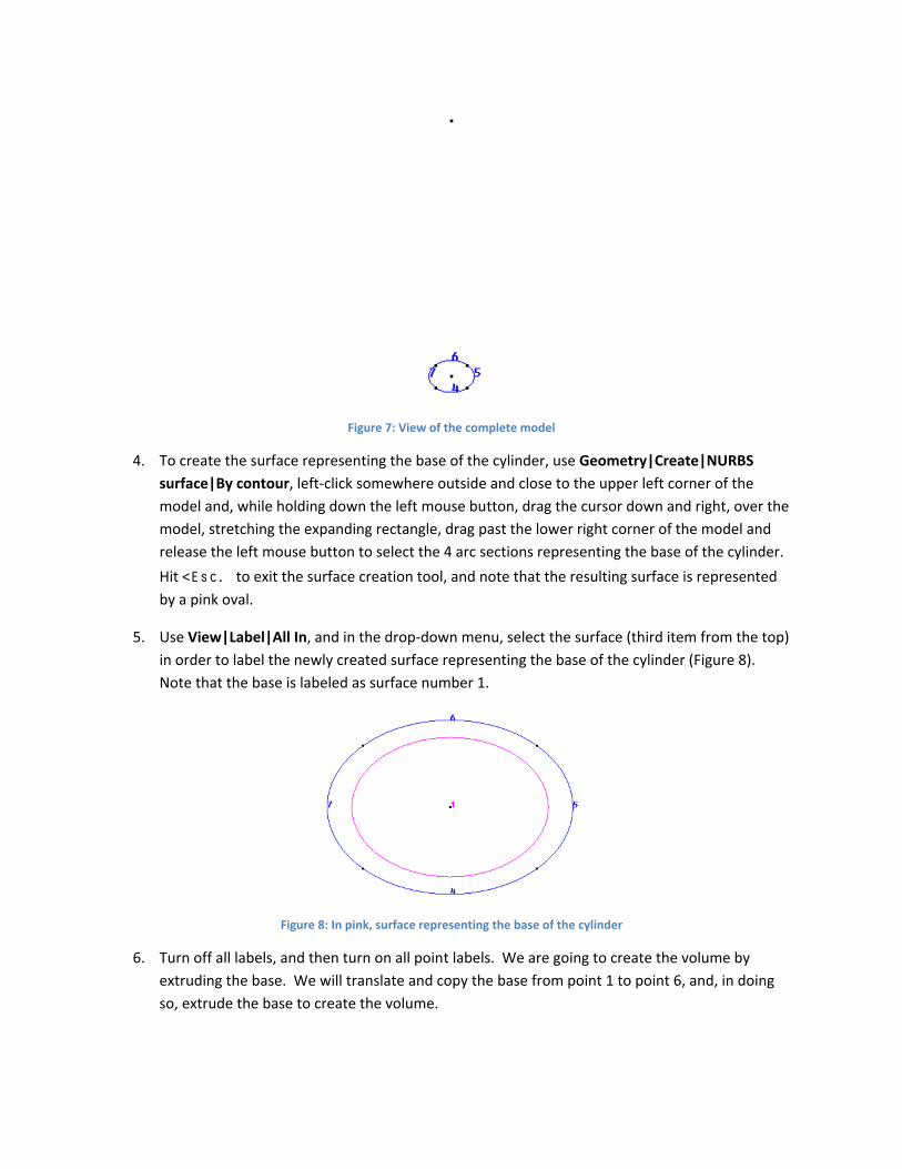
Figure 7: View of the complete model

4. To create the surface representing the base of the cylinder, use Geometry|Create|NURBS surface|By contour, left-click somewhere outside and close to the upper left corner of the model and, while holding down the left mouse button, drag the cursor down and right, over the model, stretching the expanding rectangle, drag past the lower right corner of the model and release the left mouse button to select the 4 arc sections representing the base of the cylinder.

Hit <Esc. to exit the surface creation tool, and note that the resulting surface is represented by a pink oval.

5. Use View|Label|All In, and in the drop-down menu, select the surface (third item from the top) in order to label the newly created surface representing the base of the cylinder (Figure 8). Note that the base is labeled as surface number 1.

Figure 8: In pink, surface representing the base of the cylinder

6. Turn off all labels, and then turn on all point labels. We are going to create the volume by extruding the base. We will translate and copy the base from point 1 to point 6, and, in doing so, extrude the base to create the volume.

7. Use Utilities|Copy to open the Copy dialog box. Select Surfaces for Entities types and Translation for Transformations,

8. To define the First point, click on Pick, then on point number 1 which represents the center of the base. For Second Point, click on Pick and then on point 6 of your model. Note that after each pick operation, the coordinates of that point appear in the corresponding window in the dialog box.

9. Select Volumes for Do extrude and then click on Select (Figure 9).

Figure 9: Copy dialog box showing the parameters used for base extrusion

Your cursor symbol changes to a , indicating that you must now select the surface that will be

extruded.

10. Click on the pink oval labeled surface number 1, then Hit <Esc. to end the selection of surfaces and complete the extrusion. Close the Copy dialog box and label all entities to see the 4 newly formed surfaces shown in pink and the volume shown in light blue and labeled as volume 1 (Figure 10). Use File|Save as to save your model under the name Cylinder.gid.

Figure 10: Volume and surfaces resulting from the extrusion of the base.

Part 2: Fluid flow model setup In part 2 of this tutorial, you will define the CFD problem, boundary and initial conditions and additional parameters needed for the CFD part of the calculation

Material definition 1. If your model is not open, start GID and using File|Open read the Cylinder.GID project folder.

Use Data|Problem type|CFD to indicate that you are going to set up a CFD problem. Use View|Zoom|In to magnify the details of the model.

2. Use View|label|All to label everything in the model, and select Data|Materials to open the Materials dialog box. Select Water as the material in the uppermost field of the dialog box, click

on Assign and select Volume. The cursor changes to a symbol, indicating that you must now

select a volume to which the material “Water” will be assigned.

3. Click on the cylinder volume, drawn in light blue, hit <Esc. and click on Finish to terminate the

material definition stage.

4. To verify that the right material has been assigned to the right volume, while the Materials

dialog box is still open, click on Draw and select All materials to see the current material

assignment state of the model as shown in Figure 11.

Figure 11: A representation of the volumes and their material assignment in the model

5. Click on Finish, then Close to exit material definition.

Problem data 1. Use Data|Problem Data to open the Problem data dialog box. Select the General tab.

2. Enter Cylinder in the Title field, choose EXPLICIT for the Problem type, choose No for the Turb model (Turbulence), set Sweep to any number, for instance, 100, the Relax factor to 0.8, the

Relax factor P to 0.2 and the Scheme to 0. Click on Accept data to complete the General tab

(Figure 12).

Figure 12: The General tab of Problem data

The Restart, Monitoring point, Scalar and VOF tabs should be left at their default values as shown in Figure 13.

Figure 13: The Restart, Monitoring point, Scalar and VOF tabs

3. In the Coupling tab, check the Use coupling mark. For the Coupling type, select the 3rd entry, namely “CFD (Unsteady) <-> FINAS (Dynamic).

4. Clicking on any of the Time table buttons opens 3 fields. Enter 0 for start, 1 for end, and 0.001

for the step value (Figure 14). Click on Accept data followed by Close to close the Problem

Data dialog box.

Figure 14: The coupling dialog box showing the Coupling Type and the time step specification

Interval data 1. Use Data|Interval Data to open the Interval Data dialog box. In the Control tab, set the

Number of steps to a figure greater or equal to 1000 and the Time step increment to 0.001.

2. The Gravity and Criterion temp tabs should be left at their default values (Figure 15).

Figure 15: The Control, Gravity and Criterion temp tabs of the Interval Data dialog box

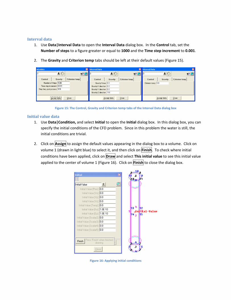
Initial value data 1. Use Data|Condition, and select Initial to open the Initial dialog box. In this dialog box, you can

specify the initial conditions of the CFD problem. Since in this problem the water is still, the initial conditions are trivial.

2. Click on Assign to assign the default values appearing in the dialog box to a volume. Click on

volume 1 (drawn in light blue) to select it, and then click on Finish. To check where initial

conditions have been applied, click on Draw and select This initial value to see this initial value

applied to the center of volume 1 (Figure 16). Click on Finish to close the dialog box.

Figure 16: Applying initial conditions

Boundary conditions 1. Use Data|Condition and select Boundary to open the Boundary dialog box. In the pull-down

menu, select FIXED-VELOCITY and set the X, Y and Z values to 0.

2. Click on Assign. You must now select all the surfaces on which this boundary condition will be

applied. In this example, the FIXED-VELOCITY boundary condition is applied to all surfaces except the base, that is a total of 5 surfaces.

3. Click on the top and the 4 lateral surfaces. Hit <Esc. or click on Finish to exit the surface

selection tool.

4. In the pull-down menu at the top of the Boundary dialog box, select FIXED-PRESSURE, and set

its value to 0. Click on Assign and click on the base of the cylinder to apply this boundary

condition to this surface, then hit <Esc. or click on Finish to exit the surface selection tool.

5. To visualize all the boundary and initial conditions, click Draw and select All conditions (Figure

17). Click on Finish to close the dialog box.

Figure 17: Summary of all initial and boundary conditions

6. Save your model as Cylinder.GID

Mesh generation In CCFD, you can use both hexahedral and tetrahedral meshes. In this example, we will create a so-called structured or mapped hexahedral mesh.

1. Continue on from the previous section or read the Cylinder.GID project file. Use Meshing|Element type|Hexahedra in order to specify your choice of elements.

2. Using View|Rotate|Isometric and View|Zoom|In to adopt a clear and detailed view of your model, enabling you to pick any line. Turn off all labels, and remember that points are represented as black dots, lines are in blue, surfaces in pink and volumes appears in light blue.

3. A mapped mesh is composed of a collection of cubes, elastically deformed to match the shape of the cylinder. We will mesh this volume as a single block. This is also called a Structured mesh for the fact that the mesh has an inherent I, J, K numbering. so that the base and top face the Bottom and Top directions and the 4 remaining surfaces face East, West, South and North. Use Meshing|Structured|Volumes. The cursor symbol changes and you can read in the bottom left of the screen that you must select six-sided volumes. Here, we have only one volume. Click on

it to select it then hit <Esc. . Exiting volume selection immediately opens an Enter value window.

4. You only need three numbers to mesh this cylinder as a stretched cube. This dialog box enables you to specify the number of subdivisions in each of the 3 Bottom-Top, East-West and South-

North directions. Enter 5, then click OK, and select a segment along, say, the East-West

direction. In fact any of the 4 arcs forming the base of the cylinder would do. As soon as you click on that line, you will notice that the color of 3 other lines, the quarter arc located opposite the one you chose, as well as the two corresponding arcs on the top lid of the cylinder turn red; meaning that they have been selected and that the number of subdivision on them has been set to 5.

5. While you are still in the line selection mode, select an arc adjacent to the one you clicked to set the number of subdivisions in the South-North direction to 5 as well (Figure 18).

Figure 18: Model after assignment of number of meshing subdivisions in the East-West and South-North directions. Note that the only remaining unassigned (blue) lines are in the Bottom-Top direction.

6. Hit <Esc> to exit the line selection mode. The Enter value window reappears. Enter 40, click

OK and select any of the 4 remaining straight blue lines to assign the number of subdivisions

along the Bottom-Top direction. Note that the remaining 3 Bottom-Top lines also turn red.

7. Hit <Esc> to exit the line selection mode. Hit <Esc> again or click on Cancel to close the Enter

value window that has opened in anticipation of new values.

8. You have now completed the subdivision assignment and are ready to generate the mesh. Use Meshing|Generate to open Enter value window. This window already contains a certain

default value. Ignore it and click on OK to generate the mesh. A window appears reporting the

progress of mesh generation, followed by an informational window reporting that 1000

hexahedral element and 1476 nodes were created. Click OK to see the resulting mesh (Figure

19).

Figure 19: Structured hexahedral mesh of the cylinder

9. Use File|Save to save the geometry (points, lines, surface and volume), all operating conditions and the mesh of your model.

Part 3: PFC3D data file preparation The PFC3D portion of the computations needs a data file describing the location, size and properties of particles.

Description of various statements in the PFC3D data file. Figure 20 shows a listing of the PFC3D data file used in this tutorial

Figure 20: PFC3D data file

Part 4: Launching the calculation In part 4 of this tutorial, you will learn to launch PFC3D with CCFD option.

1. Start GID and open the Cylinder.gid project.

2. Using Calculate|Calculate, open the FINAS-CFD dialog box. Click on Data+Exec, and after a

short time note that the Open dialog box opens. This box lists all the files located in the Cylinder.gid project with the extension “.dat“.

3. You must now read the PFC3D data file needed for the computation. Select the file

PfcCylinder.dat and click on Open (Figure 21).

Figure 21: Reading the PFC3D data file

4. After reading the PFC3D data file, a proxy program which manages communications between PFC3D and the CCFD solvers (Figure 22) is initiated.

Figure 22: Proxy program about to start

5. Clicking on Start launches the coupled PFC-CCFD computation. A PFC3D window opens on your

screen, and you will notice several commands being executed until the Pause statement at the bottom of the PFC3D data file (Figure 20) is reached (Figure 23).

Figure 23: PFC3D screen launched by the proxy program

6. Enter Continue in the command window of PFC3D to resume the computation. At pre-set time intervals, defined earlier in the Coupling General dialog box (Figure 14), PFC3D and CCFD exchange information. Use the WINDOW’s taskbar to see the CCFD screen displaying the current state of the CFD computation (Figure 24).

Figure 24: CCFD screen running in conjunction with PFC3D

7. The computation will stop at the end of 1000 time steps as specified in the Coupling tab of the Problem data dialog box (Figure 14).

End of Tutorial 1.