perturbation methods: solving dsge models with...

Perturbation methods: Solving DSGE models with Dynare

Randall Romero

The Ohio State University

First draft: April 5, 2013

Last revised: October 7, 2014

About this presentation

Dynare is a user-friendly software platform useful for solving dynamic economic models.

Dynare relies on perturbation methods to find solution to models.

The two objectives of this presentation are:

to explain the logic behind the use of perturbation methods; and

to provide a short introduction to the use of Dynare.

For illustration, we solve the Solow model and the Ramsey model.

Randall Romero (OSU) Perturbation methods and Dynare 2014 2 / 63

Outline

1 Perturbation Methods

Some math results

Perturbation in dynamic models

An example: The Solow model

Another example: The Ramsey model

2 Some Dynare basics

About Dynare

About model types

3 Examples of models in Dynare

A deterministic Solow model

A stochastic Ramsey model

Perturbation Methods

Perturbation methods

Dynare approach to solving dynamic models is based on perturbation methods.

These methods are based on Taylor’s expansions and the implicit function theorem.

In this section we review the mathematics necessary to understand perturbation methods.


Perturbation Methods Some math results

Fixed point of a function

Let f : Rn → Rn be a function. A point x∗ ∈ Rn is

called a fixed point of f if it satisfies

f (x∗) = x∗

Example: f (x) = 2√x has two fixed points:

x∗ = 0 and x∗ = 4.

x0 2 4 6 8

0

2

4

6

8

y = f(x) = 2x1/2



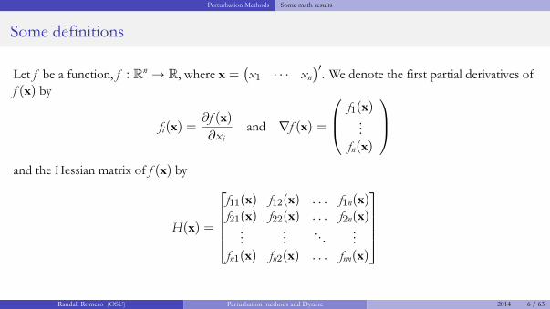
Some definitions

Let f be a function, f : Rn → R, where x =(x1 · · · xn

)′. We denote the first partial derivatives of

f (x) by

fi(x) =∂f (x)

∂xiand ∇f (x) =

f1(x)...

fn(x)

and the Hessian matrix of f (x) by

H(x) =

f11(x) f12(x) . . . f1n(x)f21(x) f22(x) . . . f2n(x)...

.... . .

...

fn1(x) fn2(x) . . . fnn(x)



Some notation

Let f be a function, f : Rn → Rm :

f (x) =

f 1(x)...

f m(x)

We denote the Jacobian of f (x) by

J(x) =

f 11 (x) f 12 (x) . . . f 1n (x)f 21 (x) f 22 (x) . . . f 2n (x)...

.... . .

...

f m1 (x) f m2 (x) . . . f mn (x)

=

∇f 1(x)′

∇f 2(x)′

...

∇f m(x)′



A partial Jacobian

Let g(x, y) be a function of vectors x ∈ Rn and y ∈ Rm , such that g : Rn+m → Rm .

Think of g as a system of m nonlinear equations on m endogenous variables y and n exogenous

variables x.

The partial Jacobians Dgx and Dgy form a partition of the Jacobian:

J(x, y) =[Dgx |Dgy

]=

g1x1 g1x2 . . . g1xng2x1 g2x2 . . . g2xn...

.... . .

...

gmx1 gmx2 . . . gmxn

g1y1 g1y2 . . . g1ymg2y1 g2y2 . . . g2ym...

.... . .

...

gmy1 gmy2 . . . gmym



Taylor’s Theorem

Taylor’s theorem, R case

Let f : [a, b] → R be a n + 1 times continuously differentiable function on (a,b), let x̄ be a point in(a,b). Then

f (x̄ + h) = f (x̄) + f (1)(x̄)h + f (2)(x̄)h2

2+ . . .+ f (n)(x̄)

hn

n!

+ f (n+1)(ξ)hn+1

(n + 1)!, ξ ∈ (x̄, x̄ + h)



Example of Taylor’s Theorem: f (x) = 2√x

Approximation of

f (x) = 2√x

around the fixed point

x∗ = 4



Taylor approximations

Taylor’s approximation, Rn case

Let f : Rn → R be a twice continuously differentiable function on a neighborhood of x. Then

f (x+ h) ≈ f (x) + [∇f (x)]′ h+ 12h

′H(x)h

is a second-order Taylor approximation of f at the point x



Taylor approximation around a fixed point

Suppose that the sequence xt+1 = f (xt) of vectors in Rn has a fixed point x∗. Then the second-orderTaylor approximation around x∗ is

xt+1− x∗ ≈ [∇f (x∗)]′ (xt − x∗) + 12(xt − x∗)′H(x)(xt − x∗)

The first-order approximation is simply

xt+1− x∗ ≈ [∇f (x∗)]′ (xt − x∗)

These expressions can be interpreted as describing “deviations from equilibrium”. Notice the

similarity of the latter expression to a VAR(1) model written as deviation from the mean (without the

stochastic term).



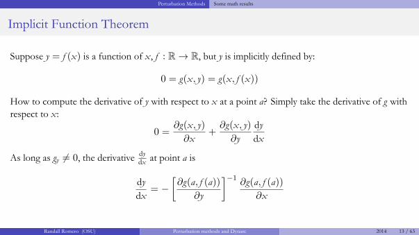
Implicit Function Theorem

Suppose y = f (x) is a function of x , f : R → R, but y is implicitly defined by:

0 = g(x, y) = g(x, f (x))

How to compute the derivative of y with respect to x at a point a? Simply take the derivative of g with

respect to x :

0 =∂g(x, y)

∂x+

∂g(x, y)

∂y

dy

dx

As long as gy 6= 0, the derivative dy

dxat point a is

dy

dx= −

[∂g(a, f (a))

∂y

]−1 ∂g(a, f (a))

∂x



Implicit Function TheoremSecond derivative

We can use 0 = gx(x, y) + gy(x, y)y′ to obtain the second derivative y′′:

0 = ∂∂x gx(x, y) + y′ ∂

∂x gy(x, y) + gy(x, y)∂∂x y

′

= gxx + gxyy′ + y′(gyx + gyyy

′) + gyy′′

Then, the second derivative is

y′′ = − 1gy

[gxx + 2gxyy

′ + gyy(y′)2

]



Implicit Function Theorem, several variables

Now suppose that y = f (x) is a function, f : Rn → Rm , but f is implicitly defined by m possibly

nonlinear functions g : Rn+m → Rm :

0 = g(x, y) =

g1(x, y)...

gm(x, y)

The Jacobian of f (x) at a point x̄ is given by

J(x̄) = −[Dgy(x̄, f (x̄))

]−1Dgx(x̄, f (x̄))

where the m × m matrix Dgy is invertible.


Perturbation Methods Perturbation in dynamic models

Regular perturbation: the basic idea

Suppose that a problem reduces to solving

f (x, ε) = 0

for x where ε is a parameter.

We assume that for each value of ε the equation has a solution for x .

Let x = x(ε) denote a smooth function such that f (x(ε), ε) = 0.

In general, we cannot solve the equation for arbitrary ε, but there may be special values of ε forwhich the equation can be solved.



Example

Consider the function

f (x(ε), ε) = x3 − εx − 1 = 0

For ε = 0, it’s easy to find a solution:

f (x(0), 0) = x3 − 1 = 0 ⇒ x(0) = 1

We will approximate solutions to

x3(ε)− εx(ε)− 1 = 0 for arbitrary ε, based onknowing x(0) = 1.

x

-1 -0.5 0 0.5 1 1.5 2

f(x, ǫ)

-2

-1

0

1

2

3

4

5

6

7

x3 - 1 →

← x3 - x - 1

x(0) = 1 x(1) = ?

x3 - ǫ x - 1



Regular perturbation: the basic idea (cont.)

If f (x, ε) and x(ε) are differentiable, and x(0) is known, we can differentiate f (x(ε), ε) = 0 toget an implicit expression for x ′(ε):

fx(x(ε), ε)x′(ε) + fε(x(ε), ε) = 0

Evaluated at known x(0), it becomes

fx(x(0), 0)x′(0) + fε(x(0), 0) = 0 ⇒ x ′(0) = − fε(x(0),0)

fx(x(0),0)

Then, the linear approximation of x(ε) for ε near zero is

x(ε) ≈ xL(ε) = x(0)− fε(x(0),0)fx(x(0),0)

ε



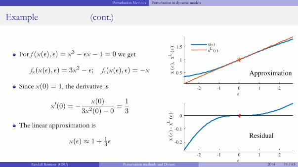
Example (cont.)

For f (x(ε), ε) = x3 − εx − 1 = 0 we get

fx(x(ε), ε) = 3x2 − ε; fε(x(ε), ε) = −x

Since x(0) = 1, the derivative is

x ′(0) = − x(0)

3x2(0)− 0=

1

3

The linear approximation is

x(ε) ≈ 1 + 13ε

ǫ

-2 -1 0 1 2

x (ǫ),

x

L (ǫ)

0.5

1

1.5

Approximation

x(ǫ)

xL (ǫ)

ǫ

-2 -1 0 1 2

x (ǫ)

- x

L (ǫ)

-0.2

-0.1

0

Residual



The economist’s problem

You have an intertemporal model with n endogenous variables xt , whose dynamics are described

by xt+1 = Ψ(xt).

You have found n equilibrium conditions of the form g(xt , xt+1) = 0.

The model is stationary, as such Ψ has a fixed point x∗ (the steady state): x∗ = Ψ(x∗).

Problem: How to analyze the dynamics of the model without an explicit solution for Ψ(x)?



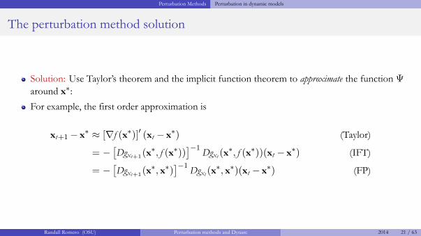
The perturbation method solution

Solution: Use Taylor’s theorem and the implicit function theorem to approximate the function Ψaround x∗:

For example, the first order approximation is

xt+1− x∗ ≈ [∇f (x∗)]′ (xt − x∗) (Taylor)

= −[Dgxt+1(x

∗, f (x∗))]−1

Dgxt (x∗, f (x∗))(xt − x∗) (IFT)

= −[Dgxt+1(x

∗, x∗)]−1

Dgxt (x∗, x∗)(xt − x∗) (FP)


Perturbation Methods An example: The Solow model

Example: Solow model

To illustrate the procedure of perturbation, we use Solow model

It has only one dynamic equation, which will make easier to see the logic



Example: Solow model

In the Solow model, capital accumulates according to:

0 = g(kt , kt+1) = sAkαt + (1− δ)kt − (1 + n)kt+1

The steady state is

k∗ =(

sAn+δ

) 11−α

Notice that in this example, the solution is trivial: kt+1 = Ψ(kt) =sA1−n

kαt + 1−δ1−n

kt . We will use this

model to illustrate the technique and to evaluate the quality of the approximation.



Finding the partial derivatives of Solow equationg(kt , kt+1) = sAkαt + (1− δ)kt − (1 + n)kt+1

derivative . . . −→ evaluated at k∗

gk = αsAkα−1t + (1− δ) α(δ + n) + 1− δ

gk′ = −(1 + n) − 1− n

gkk = α(α− 1)sAkα−2t α(α− 1)(δ + n) (k∗)−1

gkk′ = 0 0

gk′k′ = 0 0



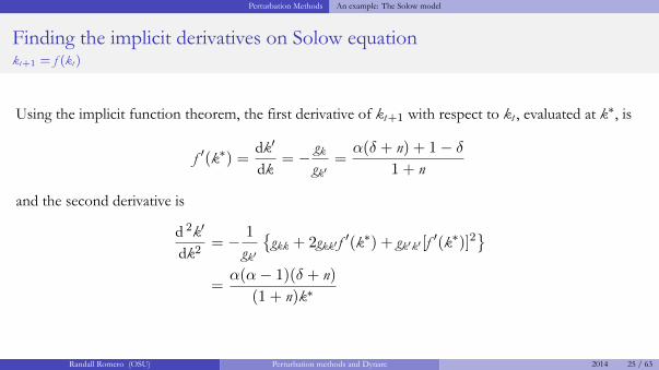
Finding the implicit derivatives on Solow equationkt+1 = f (kt)

Using the implicit function theorem, the first derivative of kt+1 with respect to kt , evaluated at k∗, is

f ′(k∗) =dk′

dk= − gk

gk′=

α(δ + n) + 1− δ

1 + n

and the second derivative is

d 2k′

dk2= − 1

gk′

{gkk + 2gkk′ f

′(k∗) + gk′k′ [f′(k∗)]2

}=

α(α− 1)(δ + n)

(1 + n)k∗



First-order approximation to Solow model

In this case

kt+1 − k∗ ≈ −[Dgkt+1(k

∗, k∗)]−1

Dgkt (k∗, k∗)(kt − k∗)

=α(δ + n) + 1− δ

1 + n(kt − k∗)

= 1+n−(1−α)(n+δ)1+n

(kt − k∗)

Notice that

∣∣∣1+n−(1−α)(n+δ)1+n

∣∣∣ < 1, so the system is stable.



Second-order approximation to Solow model

We just need to add the quadratic term to the previous approximation

kt+1 − k∗ ≈ 1+n−(1−α)(n+δ)1+n

(kt − k∗)− α(1−α)(δ+n)2(1+n)k∗ (kt − k∗)2

Let k̂ = (k− k∗)/k∗. After dividing both sides by k∗, the approximation becomes

k̂t+1 ≈ 1+n−(1−α)(n+δ)1+n

k̂t − α(1−α)(δ+n)2(1+n) k̂2t

This will converge as long as

− 1α < k̂t <

2(1+n)−(1−α)(n+δ)α(1−α)(n+δ)



Approximating the adjustment to steady state

Linear and quadratic

approximations around

k∗ = 0.51

Parameters:

s 0.10

A 1.00

α 0.40

δ 0.10

n 0.05



Approximating the impulse response function

Linear and quadratic

response to a 20%

increase in A

Parameters:

pre- post-

s 0.10 0.10

A 1.00 1.20

α 0.40 0.40

δ 0.10 0.10

n 0.05 0.05

k∗ 0.51 0.69



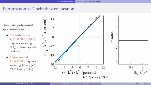
Perturbation vs Chebyshev collocation

Quadratic polynomialapproximations:

Chebyshev over

kt ∈ [0.8k∗, 1.2k∗],requires knowing

f (ki) at three specificnodes ki .

Taylor around

k∗ = 0.51 , requiresknowing k∗ = f (k∗),f ′(k∗),and f ′′(k∗)


Perturbation Methods Another example: The Ramsey model

Example: Ramsey model

The solution of the Ramsey problem is characterized by the equations 1

0 = g1(Kt ,Ct ,Kt+1,Ct+1) = Kt+1 − f (Kt) + Ct

0 = g2(Kt ,Ct ,Kt+1,Ct+1) = u′(Ct)− βu′(Ct+1)f′(Kt+1)

The perturbation method will allow us to approximate the function Ψ[Kt+1

Ct+1

]= Ψ

([Kt+1

Ct+1

])

1This example follows the presentation by Heer and Maußner 2009, pp. 77–Randall Romero (OSU) Perturbation methods and Dynare 2014 31 / 63


Finding the steady state

The steady state is given by

0 = g1(K∗,C∗,K∗,C∗) = K∗ − f (K∗) + C∗

0 = g2(K∗,C∗,K∗,C∗) = u′(C∗)− βu′(C∗)f ′(K∗)

that is, the steady state k∗, c∗ satisfies

f ′(k∗) = β−1

c∗ = f (k∗)− k∗



Finding the Jacobian

Let xt = (kt , ct)′. From the equations

0 = g1(Kt ,Ct ,Kt+1,Ct+1) = Kt+1 − f (Kt) + Ct

0 = g2(Kt ,Ct ,Kt+1,Ct+1) = u′(Ct)− βu′(Ct+1)f′(Kt+1)

we find the Jacobian of g evaluated at the steady state

J(xt , xt+1) =[Dgxt |Dgxt+1

]=

[−f ′(k∗) 1

0 u′′(c∗)1 0

−βu′(c∗)f ′′(k∗) −βu′′(c∗)f ′(k∗)

]=

[−β−1 10 u′′

1 0−βu′f ′′ −u′′

]



The first-order approximation

The first order approximation is[kt+1 − k∗

ct+1 − c∗

]= −

[1 0

−βu′f ′′ −u′′

]−1[−β−1 10 u′′

] [kt − k∗

ct − c∗

]=

[β−1 −1

− u′f ′′

u′′ 1 + βu′f ′′

u′′

] [kt − k∗

ct − c∗

]


Outline


Some math results





About Dynare

About model types




Some Dynare basics About Dynare

What is Dynare?

“Dynare is a powerful and highly customizable engine, with an intuitive front-end interface, to

solve, simulate and estimate DSGE models.”

It is a pre-processor and a collection of Matlab routines that has the great advantages of reading

DSGE model equations written almost as in an academic paper.

This not only facilitates the inputting of a model, but also enables you to easily share your code as

it is straightforward to read by anyone.



Dynare’s workflow

1.2. WHAT IS DYNARE? 3

Figure 1.1: The .mod file being read by the Dynare pre-processor, which thencalls the relevant Matlab routines to carry out the desired operations anddisplay the results.

In slightly less flowery words, it is a pre-processor and a collection of Mat-lab routines that has the great advantages of reading DSGE model equationswritten almost as in an academic paper. This not only facilitates the inputtingof a model, but also enables you to easily share your code as it is straightfor-ward to read by anyone.

Figure 1.2 gives you an overview of the way Dynare works. Basically, themodel and its related attributes, like a shock structure for instance, is writ-ten equation by equation in an editor of your choice. The resulting file willbe called the .mod file. That file is then called from Matlab. This initiatesthe Dynare pre-processor which translates the .mod file into a suitable inputfor the Matlab routines (more precisely, it creates intermediary Matlab or Cfiles which are then used by Matlab code) used to either solve or estimate themodel. Finally, results are presented in Matlab. Some more details on theinternal files generated by Dynare is given in section 4.2 in chapter 4.

Each of these steps will become clear as you read through the User Guide,but for now it may be helpful to summarize what Dynare is able to do:

Source: Mancini Griffoli 2013



What is Dynare able to do?

Compute the steady state of a model

Compute the solution of deterministic models

Compute the first and second order approximation to solutions of stochastic models

Estimate parameters of DSGE models using either a maximum likelihood or a Bayesian approach

Compute optimal policies in linear-quadratic models


Some Dynare basics About model types

A fundamental distinction

Dynare can solve both deterministic and stochastic models.

The distinction hinges on whether future shocks are known.

In deterministic models, the occurrence of all future shocks is know exactly at the time of computing

the model’s solution.

In stochastic models, only the distribution of future shocks is known.

If you only consider a first-order linear approximation of the stochastic model, or a linear model,

the two cases become practically the same, due to certainty equivalence.



Deterministic vs stochastic models

Deterministic models:

assume full information, perfect foresight, and no

uncertainty about shocks.

shocks can last one or more periods.

the solution does not require linearization: exact

path of endogenous variables.

solution is useful even when economy is far away

from steady state.

Stochastic models

assume that shocks hit today (with a surprise), but

thereafter their expected value is zero.

expected future shocks, or permanent changes in

the exogenous variables cannot be handled due to

the use of Taylor approximations around a steady

state.

solution can be poor when economy is far from

steady state.



A .mod file for a stochastic model

16 CHAPTER 3. SOLVING DSGE MODELS - BASICS

Figure 3.1: The .mod file contains five logically distinct parts.

3.4.1 The deterministic case

The model is inherited exactly as specified in the earlier description, exceptthat we no longer need the et variable, as we can make zt directly exogenous.Thus, the preamble would look like:

var y c k i l y l w r;

varexo z;

parameters beta psi delta alpha sigma epsilon;

alpha = 0.33;

beta = 0.99;

delta = 0.023;

psi = 1.75;

sigma = (0.007/(1-alpha));

epsilon = 10;

3.4.2 The stochastic case

In this case, we go back to considering the law of motion for technology, con-sisting of an exogenous shock, et. With respect to the above, we therefore

Structure of the .mod file

Source: Mancini Griffoli 2013

// This is a sample .mod file for Dynare

var y1 y2 . . . yn; // n endogenous variables

varexo x1 x2 . . . xm; // m exogenous variables

parameters φ1 φ2 . . . φp; // p parameters

φ1 = 0.25;...

φp = 0.91;model; // n equations

eq1 ;...

eqn ;

end;

initval; // n + m initial values

y1 = y1,0 ;...

xm = xm,0 ;

end;

steady;

shocks; // shocks to system

xi = xi,0 ;...

xj = xj,0 ;

end;

stoch_simul (periods=h); // stochastic simulation



Installing Dynare in Matlab: a warning

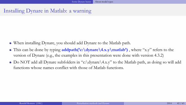
When installing Dynare, you should add Dynare to the Matlab path.

This can be done by typing addpath(’c:\dynare\4.x.y\matlab’) , where “x.y” refers to the

version of Dynare (e.g., the examples in this presentation were done with version 4.3.2)

Do NOT add all Dynare subfolders in “c:\dynare\4.x.y” to the Matlab path, as doing so will add

functions whose names conflict with those of Matlab functions.


Outline


Some math results





About Dynare

About model types




Examples of models in Dynare A deterministic Solow model

Simulating deterministic models in Dynare

When the framework is deterministic, Dynare can be used for models with the assumption of

perfect foresight.

Typically, the system is supposed to be in a state of equilibrium before a period ‘1’ when the news

of a contemporaneous or of a future shock is learned by the agents in the model.

The purpose of the simulation is to describe the reaction in anticipation of, then in reaction to

the shock, until the system returns to the old or to a new state of equilibrium.

In most models, this return to equilibrium is only an asymptotic phenomenon, which one must

approximate by an horizon of simulation far enough in the future.

Another exercise for which Dynare is well suited is to study the transition path to a new

equilibrium following a permanent shock.



The output from Dynare

oo_.endo_simul The simulated endogenous variables are available in global matrix oo_.endo_simul.

This variable stores the result of a deterministic simulation (computed by simul) or of a

stochastic simulation (computed by stoch_simul with the periods option or by

extended_path). The variables are arranged row by row, in order of declaration (as in

M_.endo_names). Note that this variable also contains initial and terminal conditions,

so it has more columns than the value of periods option.

oo_.exo_simul This variable stores the path of exogenous variables during a simulation. The variables

are arranged in columns, in order of declaration (as in M_.endo_names). Periods are in

rows. Note that this convention regarding columns and rows is the opposite of the

convention for oo_.endo_simul!



The Solow Model

In the Solow model

Production: Yt = AtKαt−1N

1−αt

Consumption: Ct = (1− s)Yt

Capital accum: Kt = sYt−1 + (1− δ)kt−1

Labor growth: Nt = (1 + n)Nt−1

The variables are de-trended: xt ≡ Xt

Nt. Model is:

yt = Atkαt−1

ct = (1− s)yt

(1 + n)kt = syt + (1− δ)kt−1

The parameters are

α ∈ (0, 1)

δ ∈ (0, 1)

s ∈ (0, 1)

n > 0

K0 given



The Solow Model: steady state

In steady state:

y∗ = Ak∗α

c∗ = (1− s)y∗

(1 + n)k∗ = sy∗ + (1− δ)k∗

The steady state values are

k∗ =(

sAn+δ

) 11−α

y∗ = A(

sAn+δ

) α1−α

c∗ = (1− s)A(

sAn+δ

) α1−α



From model to Dynare: Preamble

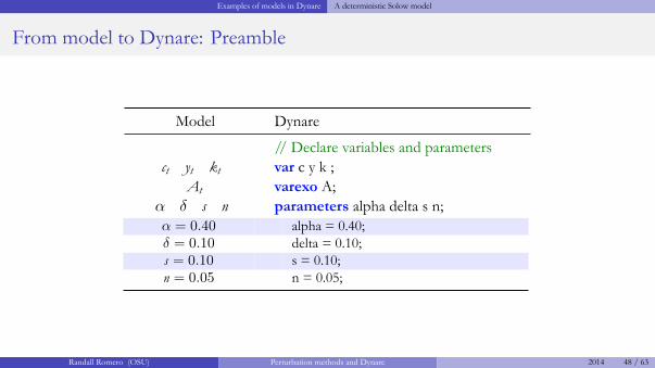
Model Dynare

// Declare variables and parameters

ct yt kt var c y k ;

At varexo A;

α δ s n parameters alpha delta s n;

α = 0.40 alpha = 0.40;

δ = 0.10 delta = 0.10;

s = 0.10 s = 0.10;

n = 0.05 n = 0.05;



From model to Dynare: Model

Model Dynare

// Declare model’s equations

model;

yt = Atkαt−1 exp(y) = A*exp(alpha*k(-1));

ct = (1− s)yt exp(c) = (1-s)*exp(y);

(1 + n)kt = syt + (1− δ)kt−1 (1+n)*exp(k) = s*exp(y(-1)) + (1-delta)*exp(k(-1));

end;

Note: writing exp(x) instead of x allows to compute impulse response function as percent

deviation from steady-state.



From model to Dynare: Initial values

Model Dynare

// Initial values

initval;

c∗ c = log(0.675);

y∗ y = log(0.75);

k∗ k = log(0.5);

A A = 1;

end;

steady;

Note: since model is written in log form, the

(approximate) steady state values in this block are also

written in log form.

The command steady forces all initial values to the

(exact) steady states.



From model to Dynare: Solving the model

Model Dynare

// Shocks

shocks;

A = 1.2 var A;

t = 4 : 6 periods 1:1;

values 1.2;

end;

steady;

// Solving

solve! simul(periods=100);

We are interested in analyzing the effect of increasing

productivity from A = 1 to A = 1.2 from period 4 toperiod 6.

We then simulate the model for 100 periods.



Results: percent deviation from steady state

Since marginal rate of savings is constant, the response

of consumption just mirrors the response on income.

There is a quick response from capital accumulation to

increased productivity; once the shock is gone, capital

adjusts slowly towards steady state.

The initial jump in capital is due to additional savings;

the slow adjustment is simply the effect of depreciation.

0 20 400

0.05

0.1

0.15

0.2c

0 20 400

0.05

0.1

0.15

0.2y

0 20 400

0.02

0.04

0.06

0.08k

0 20 400.9

1

1.1

1.2

1.3

Time path

A


Examples of models in Dynare A stochastic Ramsey model

The Ramsey model

The following model2 is a stripped down version of the celebrated model of Kydland and

Prescott (1982), who were awarded the Nobel Price in economics 2004 for their contribution to

the theory of business cycles and economic policy.

The model provides an integrated framework for studying economic fluctuations in a growing

economy.

Since it depicts an economy without money it belongs to the class of real business cycle models.

Similar models appear amongst others in the papers by Hansen (1985), by King, Plosser, and

Rebelo (1988a), and by Plosser (1989).

2This example is based on Heer and Maußner (2009, pp. 44-46)Randall Romero (OSU) Perturbation methods and Dynare 2014 53 / 63


The economy

The economy is inhabited by a representative consumer-producer who derives utility from

consumption Ct and leisure 1−Nt and uses labor Nt and capital services Kt to produce output

Yt = Zt(AtNt)1−αKα

t .

Labor augmenting technical progress at the deterministic rate a > 1 accounts for output growth:At+1 = aAt .

Stationary shocks to total factor productivity Zt induce deviations from the balanced growth path

of output: lnZt+1 = ρ lnZt + εt+1.

Capital is accumulated according to Kt+1 = (1− δ)Kt + Yt − Ct .



A Ramsey model

The representative agent solves:

maxCt ,Nt ,Kt+1

E0

[ ∞∑t=0

βt C1−ηt (1−Nt)

θ(1−η)

1− η

]

subject to

Kt+1 + Ct = Yt + (1− δ)Kt

Yt = Zt(AtNt)1−αKα

t

At+1 = aAt

lnZt+1 = ρ lnZt + εt+1

0 ≤ Ct

0 ≤ Kt+1

a ≥ 1

α ∈ (0, 1)

β ∈ (0, 1)

η > θ/(1 + θ)

θ ≥ 0

ρ ∈ (0, 1)

σ > 0

ε ∼ N(0, σ2)

K0,Z0 given



First order conditions

From the Lagrangean

L := E0

{∞∑t=0

β t C1−ηt (1−Nt)

θ(1−η)

1− η+ Λt [Yt(Nt ,Kt)− Ct − Kt+1]

}we derive the first-order conditions

wrt Ct : 0 = C−ηt (1−Nt)

θ(1−η) − Λt

wrt Nt : 0 = θC1−ηt (1−Nt)

θ(1−η)−1 − Λt(1− α)Yt

Nt

wrt Kt+1 : 0 = Λt − β Et Λt+1

(1− δ + α

Yt+1

Kt+1

)

wrt Λt : 0 = Kt+1 − (1− δ)Kt + Ct − Yt



First order conditions, stationary version

Substitute out Λt to get the system

0 = θCt − (1− α)Yt1−Nt

Nt

0 = C−ηt (1−Nt)

θ(1−η) − β Et C−ηt+1(1−Nt+1)

θ(1−η)(1− δ + αYt+1

Kt+1

)0 = Kt+1 − (1− δ)Kt + Ct − Yt

Define xt := Xt/At as a de-trended variable, then FOCs become:

0 = θct − (1− α)yt1−Nt

Nt

0 = c−ηt (1−Nt)

θ(1−η) − βa−η Et c−ηt+1(1−Nt+1)

θ(1−η)(1− δ + α yt+1

kt+1

)0 = akt+1 − (1− δ)kt + ct − yt

0 = yt − ZtN1−αt kαt



The steady state

To find the steady-state, let Zt = 1 , drop theexpectation operator:

0 = θc − (1− α)y 1−NN

0 = 1− βa−η(1− δ + α y

k

)0 = (a + δ − 1)k+ c − y

0 = y −N1−αkα

The (recursive) solution is:

N∗ ={1 + θ

1−α

[aη−β(1−δ)+αβ(1−a−δ)

aη−β(1−δ)

]}−1

k∗ =[

αβaη−β(1−δ)

] 11−α

N∗

y∗ = N∗1−αK∗α

c∗ = y∗ − (a + δ − 1)k∗



From model to Dynare: Preamble

Model Dynare

// Declare variables and parameters

ct yt kt+1 Nt Zt var c y k N Z;

kt predetermined_variables k;

εt+1 varexo e;

a α β δ η θ ρ σ parameters a alpha beta delta eta theta rho sigma;

a = 1.005 a = 1.005;

α = 0.27 alpha = 0.27;

β = 0.994 beta = 0.994;

δ = 0.011 delta = 0.011;

η = 2.0 eta = 2.0;

θ = 5.81 theta = 5.81;

ρ = 0.90 rho = 0.90;

σ = 0.0072 sigma = 0.0072;

N∗ = 0.13 Nstar = 0.13;



Dynare assumes that all variables are determined at t .

But in this model kt is not decided at time t , but at t − 1.

To alert Dynare about this, we need the line predetermined_variables k;.



From model to Dynare: Model

Model Dynare

// Declare model’s equations

model;

θct = (1− α)yt1−Nt

Nttheta*c = (1-alpha)*y*(1-N)/N;

yt = akt+1 − (1− δ)kt + ct y = a*k(+1) - (1-delta)*k +c;

yt = ZtN1−αt kαt y = Z*Nˆ(1-alpha)*kˆalpha;

c−ηt (1−Nt)

θ(1−η) =

βa−η Et c−ηt+1(1−Nt+1)

θ(1−η)(1− δ + α yt+1

kt+1

) cˆ(-eta)*(1-N)ˆ(theta*(1-eta)) =

beta*aˆ(-eta)*c(+1)ˆ(-eta) * (1-N(+1))ˆ(theta*(1-eta))

*(1-delta + alpha*y(+1)/k(+1));

lnZt = ρ lnZt−1 + εt ln(Z) = rho*ln(Z(-1)) + e;

end;



From model to Dynare: Initial values

Model Dynare

// Initial values

initval;

c∗ c = 0.25;

y∗ y = 0.30;

k∗ k = 3.02;

N∗ N = 0.13;

Z = 1.00;

E εt e = 0;

end;

steady;

check;

The (approximate) numeric values of the steady state are

computed separately using the analytical formulas.

The command steady forces all initial values to the (exact) steady

states.

The command check ...



References

Adjemian, Stéphane et al. (2013). Dynare Reference Manual. 4.3.2. Centre pour la Reserche

Economique et ses Applications. URL:

http://www.dynare.org/wp-repo/dynarewp001.pdf.Heer, Burkhard and Alfred Maußner (2009). Dynamic General Equilibrium Modeling. Computational

Methods and Applications. 2nd ed. Springer. ISBN: 978-3-540-85684-9.

Juth, Kenneth L. (1998). Numerical Methods in Economics. MIT Press. ISBN: 978-0-262-10071-7.

Mancini Griffoli, Tommaso (2013). DYNARE User Guide. An introduction to the solution & estimation

of DSGE models. v4. URL:

http://www.dynare.org/documentation-and-support/user-guide.


http://www.dynare.org/wp-repo/dynarewp001.pdf

http://www.dynare.org/documentation-and-support/user-guide

perturbation methods: solving dsge models with...

Documents