PERFORMANCE OF SINGLE AND DOUBLE SILLS

FOR STEEP CIRCULAR CULVERTS

by

Manam V. P. Rao, Robert J. Brandes

and Frank D. Masch

Research Report Number 92 -5 F

Performance of Circular Culverts on Steep Grades

Project 3-5-66-92

Conducted for

The Texas Highway Department

In Cooperation with the

U. S. Department of Transportation, Federal Highway Administration

by

CENTER FOR HIGHWAY RESEARCH

THE UNIVERSITY OF TEXAS AUSTIN. TEXAS

January 1971

The oplnlOns, findings and conclusions expressed in this publication are those of the authors and not necessarily those of the Federal Highway Administration.

PREFACE

The research reported herein is a study of the performance of

single and double sills as a means of producing uniform distribution of

flow to the channel downstream of steep circular culverts. All experimental

work has been carried out on 18 -inch diameter corrugated metal and

concrete pipe culverts. Experiments were conducted to determine single

and double sill heightl sand locationl s within the standard Texas Highway

Department wing walls to uniformly distribute culvert flow to the down­

stream channel.

The study was initiated under an agreement between the Texas

Highway Department~ the Federal Highway Administration and the Center

for Highway Research of The University of Texas at Austin. Special

acknowledgement is made to Messrs. Sam Fox and Dwight Reagan of the

Texas Highway Department and Messrs. Frank Johnson and Edward

Kristaponis of the Federal Highway Administration for their valuable

suggestions and comments during the investigation.

Special thanks are also due to Armco Metal Pipe Corp. and

Gifford-Hill Pipe Co. for providing the corrugated metal and concrete

pipe respectively used in this study. The authors also wish to thank

Messrs. A. C. Radhakrishnan, A. Sundar and Kenneth Shuler for their

iii

assistance in construction of the models and the collection of the data.

Finally, the authors wish to thank Mrs. Joyce N. Crum for typing the

manuscript and The University of Texas Bureau of Engineering Research

for assistance with drafting.

iv

ABSTRACT

The hydraulic performance of steep sloped circular culverts was

investigated experimentally using 18-inch diameter corrugated metal and

concrete pipe culvert models of different geometrical configurations. One

of the effect means found to dissipate the energy of supercritical flows in

steep culverts was to force a hydraulic jump to form inside of the culvert

pipe by placing a sill within the flared wing walls of the culvert. Although

some amount of energy was dissipated by the jump, there still remained the

problem of high velocity concentrations in the central region of the down­

stream channel following the nappe from the jump producing sill. The use

of two sills in such cases accomplished more energy dis sipation due to the

fact that the energy of the nappe was dissipated in the pool created by the

second sill. Furthermore, the flow was dis tributed in the downstream

channel more evenly in a shorter distance.

The primary objectives of this investigation was to determine the

height and location of the jump producing sill for different culvert geometries

over a broad range of discharge factors and to determine the best double sill

configuration that would produce uniformly distributed flow in the downstream

channel.

Data were collected on water surface profiles, jump locations within

the culvert pipe, transverse depths and velocity profiles in the downstream

v

channel, and head water depths for various discharge factors ranging up to

a maximum of 6. 5 for different culvert geometries. The measured water

surface profiles and jump locations were matched with the computed values.

Energy levels in the downstream channel produced by sills were compared

to the corresponding energy levels for the case of "no sills". The reductions

of velocity concentrations in the downs tream channel due to the sills were

presented as graphical relationships between different dimensionless para­

meters pertaining to the geometry of the sills and the flow conditions.

VI

SUMMARY

The main objective of this research report has been to study the

performance of single and double sills as means of producing uniform

distribution of flow in channels downstream of steep circular culverts. In

particular, the study involved the experimental determination of the height

and location of single and double sills placed within standard Texas High­

way Department wing walls for different culvert geometries and a range of

discharge factors. For the double sill arrangement, the best configurations

(locations and heights) that would produce a uniform flow distribution in the

downstream channel were determined.

Tests were conducted on 18 -inch diameter corrugated metal and concrete

culverts for discharge factors, Q/D 2 • 5 , up to 6.5. Water surface profiles,

jump locations, transverse depth and velocity profiles in the downstream

channel were measured to evaluate the performance of the sill/ s.

Although a single sill can be used to force a jump inside a culvert, more

efficient performance can be obtained with two sills. The first sill serves to

produce a jump while the second creates a pool to dissipate the energy of the

falling jet from the first sill and to provide a more uniform distribution of

flow in the downstream channel.

With a two sill arrangement, extensive data on downstream depths and

velocity distributions for different double sill configurations were collected

vii

in order to select the best combinations of sill heights and locations.

Design criteria for these two parameters were recommended for the

corrugated metal and concrete pipe culverts.

viii

IMPLEMENTATION STATEMENT

The research indicated that the relationships between the head water

depth and the discharge factor for corrugated metal and concrete pipe culverts

operating under ventilated conditions and with sharp edged entrances were

identical up to a value of Q/D2 . 5 = 2.5. Within the range of discharge factors

2. 5 ~ Q/D2 . 5 ~ 4.5, corrugated pipe culverts could be expected to display

slug and mixture control. The concrete pipe culverts operated under orifice

control up to discharge factors equal to 6.5.

It appeared from the tes ts on corrugated metal pipe culverts that the

hydraulic jump was influenced more by a rough horizontal Unit 3 and the

sharp break in grade whereas the jump position in concrete pipe culverts was

affected very little by these factors for operation under the same conditions.

A one-dimensional method of analysis to predict water surface profiles

and jump locations was found to generally yield satisfactory results provided

that the upstream control, downstream control and the friction factor for the

pipe were well defined. It has been recommended that the downstream control

be taken as the sum of mid-sill height, head over the sill as computed from

standard weir formulas, and the velocity head at the pipe outlet.

The study also indicated that two sills were more effective than a single

sill in reducing high velocity concentrations in the downstream channel. The

more effective double sill configurations were found to be associated with

greater sill spacings and smaller end sill heights. ix

Tests showed that the two sills should be placed at distances of 1. 5

and 3.0 pipe diameters from the culvert outlet for steep corrugated metal

pipe culverts. For concrete pipe culverts, the recommended distances

are 1. 5 and 4.6 pipe diameters. The required height of the first sill can

be determined from considerations of jump formation but never higher

than O. 8D whereas the height of the end sill should be of the order of O. l6D.

x

TABLE OF CONTENTS

Page

PREFACE. iii

ABSTRACT v

SUMMARY vii

IMPLEMENTATION STATEMENT. ix

LIST OF FIGURES. xiii

LIST OF TABLES • xvi

LIST OF SYMBOLS. xviii

INTRODUCTION. 1

Objectives and Scope. 3 Literature • 5

EXPERIMENTAL PROGRAM 7

Model Setups 7 Experim.ental Procedure for Single and Double Sill Tests 13

ANALYTICAL CONSIDERATIONS. 18

Hydraulic Jum.p 20 Surface Flow Profiles 21 Hydraulic Jum.p Location . 23

ANALYSIS OF RESULTS AND DISCUSSION. 25

Head Water - Discharge Relationship • 26 Single Sill Investigations 28 Characteristics of the Hydraulic Jum.p in Circular Culverts. 34 Hydraulic Jump Location • 34

xi

Double Sill Tests on Corrugated Metal Pipe Models Double Sill Tests on Concrete Pipe Models

SUMMARY AND CONCLUSIONS

REFERENCES .

APPENDIX

xii

Page

48 66

80

84

85

LIST OF FIGURES

Figure Title

2-1 Schematic Sketch of the Experimental Setup.

2-2 Photograph of Experimental Setup C

2-3 Photograph of Experimental Setup G

2-4 Schematic Sketch for the Double Sill Tests

3-1 Definition Sketch of the Variables

4-1 Head water Depth - Discharge Factor Relationship for

Corrugated Metal and Concrete Pipe Culverts

4-2

4-3

4-4

4-5

4-6

4-7

4-8

4-9

4-10

4-11

Relationship between s/L3 and L3/E3 (End Sills)

Relationship between s/L3 and L3/E3 (Mid Sills) •

Relationship between s/L3 and Y 3/L3 (End Sills) •

Relationship between s/L3 and Y 3/L3 (Mid Sills) .

Characteristics of the Hydraulic Jump.

Froude Number as a Function of Energy Loss and

Jump Efficienc y •

Measured and Computed Surface Profiles - Setup A

Measured and Computed Surface Profiles - Setup B

Measured and Computed Surface Profiles - Setup B

Measured and Computed Surface Profiles - Setup D •

xiii

Page

8

11

11

16

19

27

30

31

32

33

35

36

44

45

46

47

Figure Title

4-12 Depth Distributions for Different Sill Configurations

(Q/D 2 • 5 = 1.5).

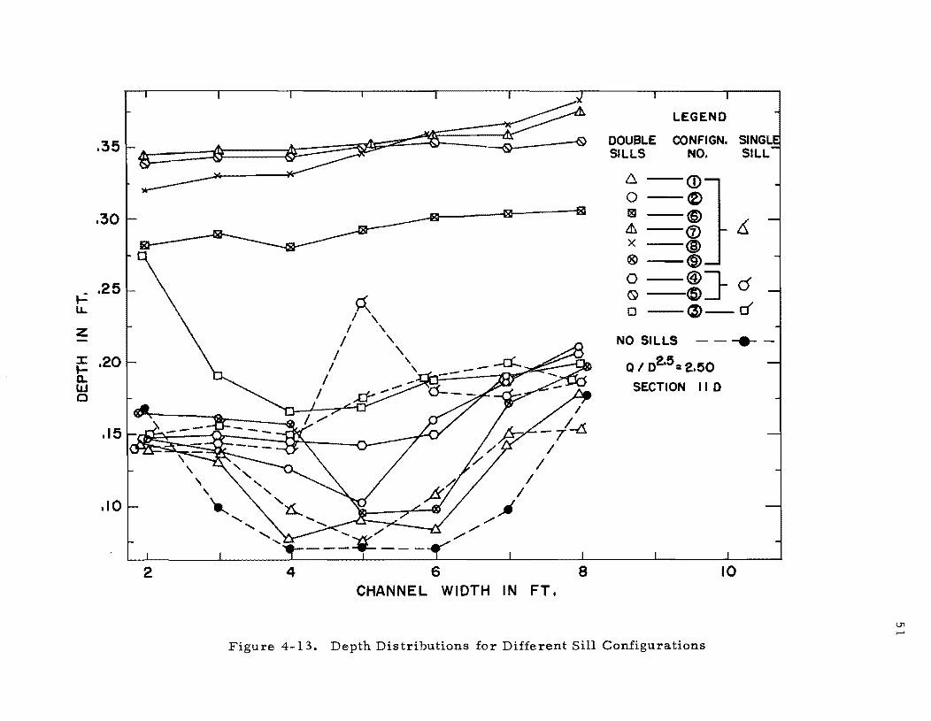
4-13 Depth Distributions for Different Sill Configurations

(Q/D2 • 5 2.5).

4-14 Depth Distributions for Different Sill Configurations

(Q/D2• 5 = 3.5) •

4-15 Depth Distributions for Different Sill Configurations

(Q/D 2 • 5 4.0).

4-16 Dowl1streanl Channel Depth Variation with Relative

Sill Spacing

4-17

4-18

4-19

4-20

4-21

4-22

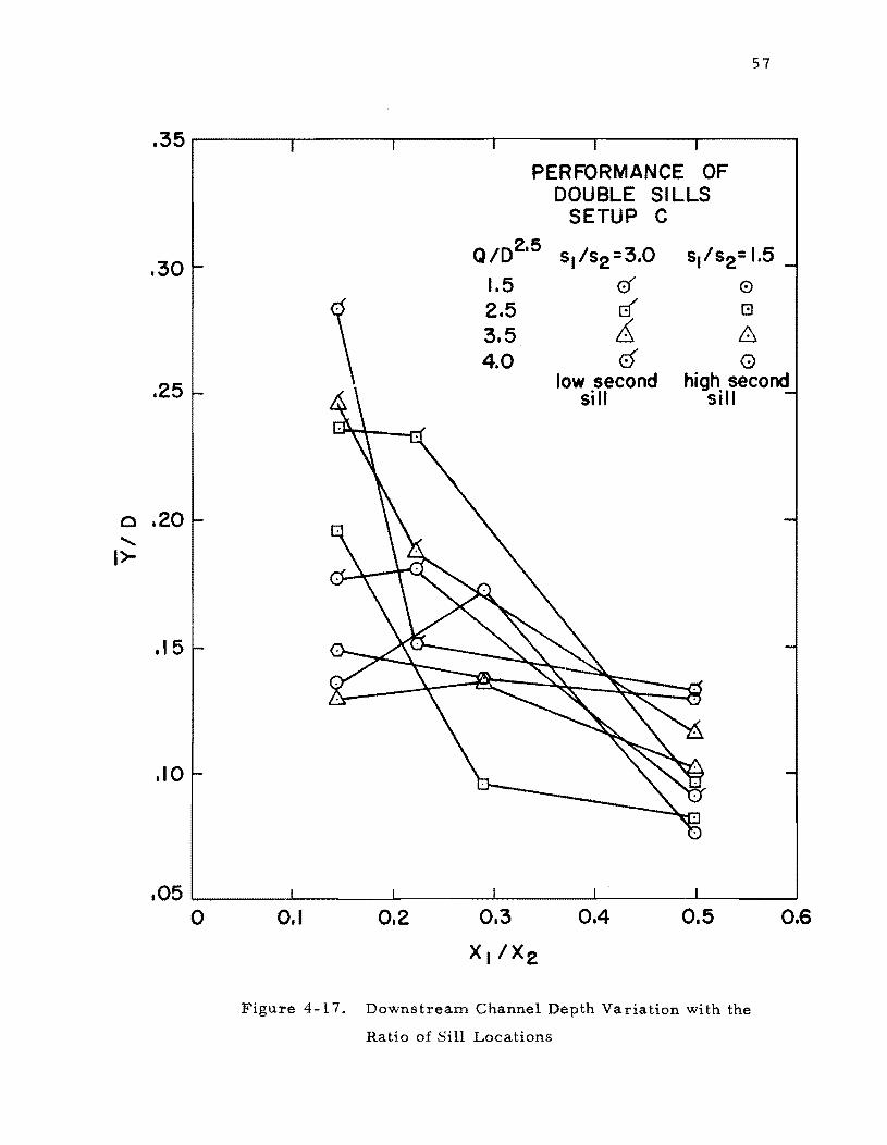
Downs treanl Channel Depth Variation with the Ratio of

Sill Locations

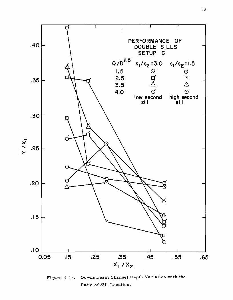
Downs treanl Channel Depth Variation with the Ratio of

Sill Locations.

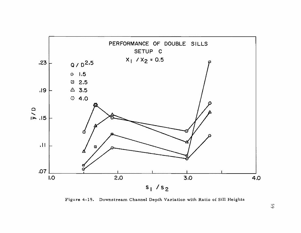
Downstreanl Channel Depth Variation with the Ratio of

Sill Heights

Relationship between Channel and Pipe Froudian NUnlbers

for Different Sill Configurations

Downstreanl Channel Transverse Depth Profiles (Setup D)

Downstreanl Channel Transverse Velocity Profiles

(Setup D) .

Page

50

51

52

53

56

57

58

59

61

68

69

4-23 Downstreanl Channel Transverse Depth Profiles (Setup E) 70

4-24 Downstreanl Channel Transverse Depth Profiles (Setup E) 71

4-25 Downstreanl Channel Transverse Velocity Profiles

(Setup E) •

xiv

72

Figu re Ti He

4-26 DownstreaITl Channel Transverse Depth Profiles (Setup F)

4-27 DownstreaITl Channel Transverse Depth Profiles (Setup F)

4-28 DownstreaITl Channel Transverse Velocity Profiles

(Setup F) •

4-2:9 DownstreaITl Channel Transverse Depth Profiles (Setup G).

4-30 DownstreaITl Channel Transverse Depth Profiles (Setup G).

4-31 DownstreaITl Channel Transverse Velocity Profiles

(Setup G) •

xv

Page

73

74

75

76

77

78

LIST OF TABLES

Table Title

2-1 Summary of the Different Culvert Setups

2-2 Discharge Ratios Used in Model Tests

4-1 Summary of Computer and Experimental Model Results

(Corrugated Metal Pipe Setup A)

4-2 Summary of Computer and Experimental Model Results

(Corrugated Metal Pipe Setups B and C) .

4-3 Geometry of the Double Sill Configurations.

4-4 Summary of Results on Double Sill Performance

(Test Section at lID) •

4-5 Summary of Results on Double Sill Performance

(Test Section at 8D)

4-6 Percentage Reduction in the Total Energy by the Use of

Double Sills •

4-7 Summary of Results on Energy Dissipation.

A-I Head Water Depth and Discharge Data for Different

Culvert Setups

A-2

A-3

A-4

Surface Profile Data - Setup A (Q/D 2 • 5

Surface Profile Data - Setup A (Q/D 2 • 5

2.0)

2. 5)

Surface Profile Data - Setup A (Q/D2 • 5 = 3.0)

xvi

Page

10

14

41

42

55

63

64

65

79

86

87

88

89

Table

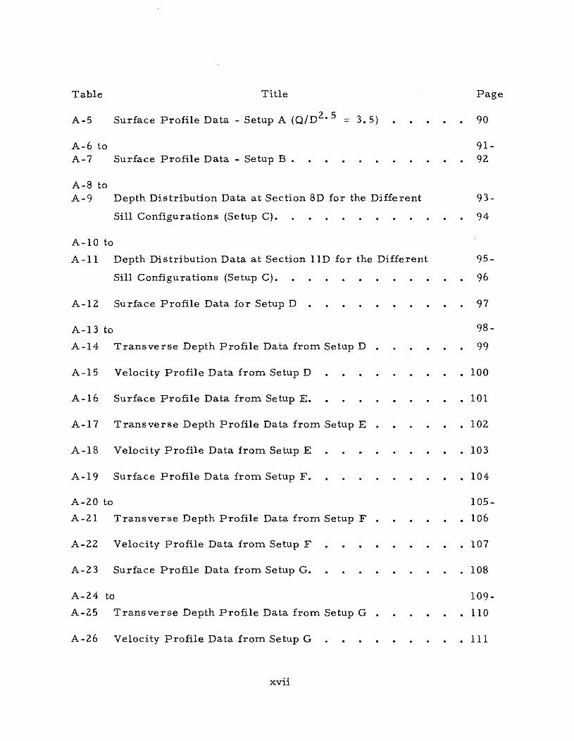
A-5

A-6 to A-7

A-8 to A-9

A-lO to

A-ll

A-12

A-13 to

A-14

A-15

A-16

A-17

A-18

A-19

A-20 to

A-2l

A-22

A-23

Title

Surface Profile Data - Setup A (Q/D2 • 5 3.5)

Surface Profile Data - Setup B •

Depth Distribution Data at Section 8D for the Different

Sill Configurations (Setup C).

Depth Distribution Data at Section lID for the Different

Sill Configurations (Setup C).

Surface Profile Data for Setup D

Transverse Depth Profile Data from Setup D •

Velocity Profile Data from Setup D

Surface Profile Data from Setup E.

Transverse Depth Profile Data from Setup E •

Velocity Profile Data from Setup E

Surface Profile Data from Setup F.

Transverse Depth Profile Data from Setup F .

Velocity Profile Data from Setup F

Surface Profile Data from Setup G.

A-24 to

A-25 Transverse Depth Profile Data from Setup G •

A-26 Velocity Profile Data from Setup G

xvii

Page

90

91-92

93-

94

95-

96

97

98-

99

• 100

• 101

• 102

• 103

• 104

105-

• 106

• 107

• 108

109-

• 110

· III

B

D

E

E3

AE

f

g

H

H, H 0 s

AH

HW

L l , L2

, L3

n

Q

R

sl' s 2

S1' S2' S3

Sf

LIST OF SYMBOLS

Width of the downstream channel.

Pi pe diame te r.

Specific energy.

Specific energy at the beginning of Unit 3.

Difference in specific energy.

Friction factor.

Acceleration due to gravity.

Total energy.

Total energy in the downstream channel at a given section

for the cases of 'no sill' and 'with sills ' respectively.

Difference in total energy.

Head water depth.

Lengths of Units 1, 2 and 3 respectively.

Manning's n.

Discharge.

Hydraulic mean radius.

Sill heights.

Slope s of Units 1, 2 and 3 respectively.

Friction slope.

xviii

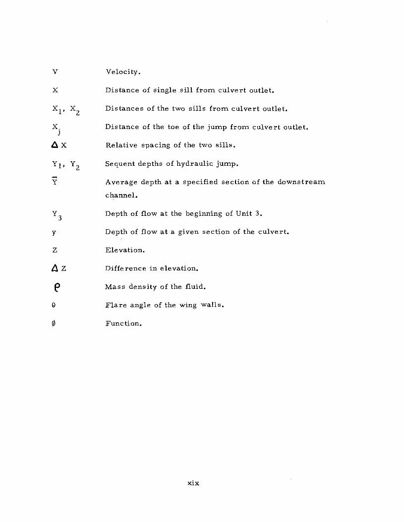
v

X

Xl' xz X.

J

Ax

Y I' YZ

Y

y

z

Az

Velocity.

Distance of single sill from culvert outlet.

Distances of the two sills from culvert outlet.

Distance of the toe of the jump from culvert outlet.

Relati ve spacing of the two sills.

Sequent depths of hydraulic jump.

Average depth at a specified section of the downstream

channel.

Depth of flow at the beginning of Unit 3.

Depth of flow at a given section of the culvert.

Elevation.

Diffe rence in elevation.

Mass density of the fluid.

Flare angle of the wing walls.

Function.

xix

CHAPTER I

INT RODUCTION

The prediction of the hydraulic perforInance of culverts on Inoderate

to steep slopes and the subsequent dissipation of energy at the culvert

outlets are essential parts of the design of highway croSS drainage systeIns.

A satisfactory design Inust provide an adequate opening to pass flows with­

out excessive build-up of water at the culvert inlet and at the saIne tiIne

insure a safe and even velocity distribution at the end of the downstreaIn

wing walls as a safeguard against scour. A design which Ineets these

requireInents should lead to IniniInuIn Inaintenance costs and efficient

operation over a broad range of flows.

The control of the exit velocity froIn culverts in which supercritical

flows develop is the principal design issue of concern in this investigation.

An econOInical Inethod for Inodifying the energy levels in the flow leaving

the culvert is sought to produce a reasonably uniforIn distribution of flow

to the downstreaIn channel. This would Inake it possible to eliIninate high

velocity flow concentrations and IniniInize potential scour probleIns.

The design of energy dis sipators is not new to highway engineers

and there are several standard types used where high velocity flows Inay

be expected. In Inost cases the creation of a hydraulic jUInp is an essential

1

feature of the energy dissipator. Because of the excessive length.

appertunances within the basin. complex shapes and difficulties in

construction many of these basins are not economically practical.

2

One effective means for dissipating energy at the end of a culvert

is to force a hydraulic jump to form with a sill located downstream of the

culvert exit. Such a sill not only provides the additional downstream force

necessary for jump formation but also aids in distributing the flow uniformly

across the width of the downstream channel. Without a sill supercritical

flow from a culvert generally maintains the characteristics of a high

velocity jet extending for considerable distances into the downstream

channel. At high discharges. however. a single sill capable of forcing

a hydraulic jump may become excessively high and since it raises the

water level above the tail water channel it may again produce a potential

scour problem as the flow spills over the sill.

More efficient performance and the production of a hydraulic jump

over a broader range of flows can be accomplished by the use of double

sills. The first sill serves to produce the force necessary to force the

jump while the downstream sill creates a pool for the dissipation of the

energy of the falling flow from the first sill and serves to distribute the

flow more uniformly to the downstream channel. It is the performance of

single and double sills over a broad range of discharges and different

culvert configurations that forms the basis for this investigation.

Objectives and Scope

The main objectives of this study are as follows:

1. Determine the sill height and sill location within the standard Texas Highway Department (THD) 30 0 flared wing walls neces sary to force a hydraulic jump as a function of the discharge and culvert geometry for l8-inch corrugated metal and concrete pipe culverts.

2. Investigate the effectiveness of two sills used simultaneously within standard THD 30 0 flared wing walls and determine the most desirable double sill configuration from the stand point of uniformity of the exit velocity.

3. Compare flow patterns in the downstream channel for conditions of no sill, a single sill, and double sills and estimate the energy dissipation in order to compare the effectiveness of the various sill configurations.

3

Although not primary objectives of this study other necessary data to fully

evaluate the sill configurations were collected. These data included:

1. Determination of the head water - discharge relationship for 18 -inch corrugated metal and concrete pipe culverts over the range of discharges used in the tests.

2. Prediction of the water surface profiles and jump locations within the culvert for given discharges, culvert geometry and sill configuration.

For each culvert configuration and discharge ratio, minimum sill

height/ s required to force a hydraulic jump were determined. The efficacy

of the double sill arrangement over a single sill is studied by comparing

4

the transverse depth and velocity distributions at sections downstreaITl of

the sills over the full range of discharge factors and sill locations. This

cOITlparative data for different sill arrangeITlents over a wide range of

discharge ratios were useful not only in the deterITlination of the energy

levels in the downstreaITl channel but also in the appropriate selection of

a double sill arrangeITlent for the corrugated ITletal and concrete pipe

culverts. These data were used to deterITline the effectiveness of the

double sill configuration relative to the single sill. The data were useful

also in estiITlating energy levels in the downstreaITl channel and the distance

froITl the various sills at which uniforITl flow was re-established in the

channel.

Only one type of sill was used for all the experiITlental tests.

Rectangular sill/ s uniforITl in both height and thickness were placed vertically

across the entire width of the channel between the flared wing walls and

perpendicular to the longitudinal axis of the culvert. Different sill height/ s

were used in a trial process to deterITline the sill height/s and location/s

that would force a stabilized hydraulic jUITlP upstreaITl of the culvert outlet

for a given discharge factor and culvert geoITletry.

Throughout the entire experiITlental portion of the study visual

observations were ITlade on the flow patterns in the vicinity of the sill/ s

located at various positions. The water surface profiles of the flow

iITlITlediately upstreaITl and over the sill/ s, the flow concentrations, and

5

the effectiveness of the sill/ s in the spreading and distributing the flow

across the width of the channel were observed. All these factors entered

in the selection of the most effective combination of sill height/ sand

location/ s.

The range of variables used in these tests are near the upper limits

for situations encountered in practice except for culverts with improved

inlets where the discharge ratios can be significantly higher. The test

conditions are believed to produce flow rates and Froude numbers in the

realm of those encountered in practice. This together with the fact that

scale effects are minimized in the large models should improve confidence

in the application of the se re s ults to prototype ins tallations.

Literature

A detailed review of the literature as it relates to culvert performance

and energy dissipators has been presented previously in Reports 92-2 and

92-4, [Refs. 1, 2] respectively. Since these reports were previously

submitted under Project 3-5-66-92 no attempt will be made to repeat this

review. Since Report 92 -4 [Ref. 2], a paper by McDonald in 1969 [Ref. 3]

described an investigation to determine the performance of a hook-type

energy dissipator used in large culverts operating with free outlet conditions.

In the McDonald work the best configuration of energy dissipator (i. e., best

location of staggered hooks downstream from the culvert outlet, their

6

thickness and spacing, end sill height, and sill opening) was determined

by experimental testing and comparisons of velocity reductions obtained

for each of the few configurations tested.

CHAPTER II

EXPERIMENTAL PROGRAM

All the experimental tests in this study were conducted on 18-inch dia­

meter corrugated metal and concrete pipe culvert models. For each model

setup and discharge ratio, data were collected on water surface profiles,

head water depths, hydraulic jump locations, sill height/ sand location/ s

and transverse depths and velocity profiles in the downstream channel. These

data were collected for the range of discharge factors, 1.5 6.5

and for steep culvert slopes of 8 and 10 percent for each type of culvert. The

inlet for all the models was of the sharp edge type and the culvert outlet was

followed by standard THD wing walls set at 300 flare to the culvert axis.

In each of the seven geometric configurations tested, the Unit 2 length

of the culvert, L 2 , was set on a steep grade. In Setups A, B, E and G, Unit

2 was followed by a short length, L 3, of horizontally placed pipe, (Unit 3).

In Setup A, a full broken back culvert configuration was tested. A detailed

description of each of these setups is given in the following section and

pe rtinent dimensions are summarized in Table 2 -1.

Model Setups

A schematic sketch of the head tank, culvert model and tail water

channel is shown in Figure 2-1. The hand tank was made of 3/4 inch

7

HEAD TANK 22' x e' x s'

.... --- Unit 2 t I

'++If+oL-----::~---..... Unit I

.......... STILLING SCREENS VALVES

-WEIR

RESERVOIR

le" DIA

--

I~~} TEST SECTIONS

--~s.9'-1 /

DOWNSTREAM CHANNEL

- --RETURN CHANNEL

Figure 2 -1. Schematic Sketch of the Experimental Setup

9

plywood and was 22 feet long, 8 feet wide and 6 feet deep. Two pumps

each capable of delivering 4,000 gpm supplied water to the head tank

through two 14-inch diameter pipe lines with regulating valves. The

head tank contained stilling screens to quieten the initial disturbance at

the entrance and to smooth the approaching flow upstream of the culvert

inlet. The depth of water in the head tank was measured with four piezo­

meters connected to taps located in the bottom of the tank and spaced one

foot apart along the central flow line upstream of the culve rt inlet.

Dimensions of the various te st setups are summarized in Table 2-1.

Figures 2-2 and 2-3 show overall views of corrugated metal and concrete

pipe corresponding to Setups C and G, respectively. Variations in the slope

of the middle section of the culvert were obtained by adjusting the cradle

supports to required elevations along the length of the model. Where

changes in the total length of the culvert model were made the tail water

channel was shortened or lengthened as to provide a closed recirculating

system. The water surface profiles in the corrugated metal pipe were

measured with pre ssure taps located along the length of the pipe and

connected to a battery of manometers. For the concrete pipe one-inch

diameter holes were drilled at one-foot intervals along the top of the pipe

and an electrical point gage equipped with neon bulb was used to measure

the water surface profiles. In the concrete pipe additional side holes were

drilled at regular intervals to supplement observations of the water surface

profile and hydraulic jump locations.

TABLE 2-1. SUMMARY OF THE DIFFERENT CULVERT SETUPS

Designation Sloping Lengths of the Individual Slopes of the Individual Units Size and the Units in Feet In Feet ner Foot Material of of the

Ll L2 L3 Sl S2 S3 the Pipe Setup Unit I Unit 2 Unit 3 Unit 1 Unit 2 Unit 3

A 5. 3 77.7 11. 3 0.0 .079 0.0 Corrugated

B 0.0 63.7 11. 3 0.0 .098 0.0 Metal Pipe

C 0.0 63.7 0.0 0.0 .098 0.0 18 -inch Diameter

D 0.0 78.0 0.0 0.0 .080 0.0 Concrete Pipe

E 0.0 78.0 12.0 0.0 .080 0.0 18-inch

F 0.0 60.0 0.0 0.0 • 104 0.0 Diameter

G 0.0 60.0 12.0 0.0 . 104 0.0

..

12

The wing walls at the outlet of the culvert also were Illade of plywood

and flared at an angle of 30 0 froIll the central flow line to conforIll with

THD standards. Provisions were Illade for placing sills within the wing

walls at various distances downstreaIll of the culvert outlet. The range of

sill locations frOIll the culvert outlet varied up to 4.6D or a IllaxiIlluIll

distance of 6.9 feet. The wing walls were followed by a tail water channel

9.8 feet wide which led water away froIll the culvert and into a return channel.

A calibrated 15" high sharp cres ted weir located in the 4-foot return channel

was used to deterIlline the flow rates through the culvert Illodels. In all

cases the invert of the culvert at the outlet was set to conforIll with the

elevation of the downstreaIll tail water channel.

Rectangular plywood sills that spanned the width of the outlet channel

between the wing walls were used to force the hydraulic jUIllp. The sill

length was equal to the width of the outlet channel at the particular location

between the wing walls. Vertical braces were fixed to the wing walls and

also at the central part of the outlet channel to hold the sills in an upright

position and perpendicular to the flow. Selection of the proper sill/ s to

stabilize a jUIllP was a trial and error process using an assortIllent of

varying sill heights. A point gage was used to Illeasure water depths above

the sill/ s and in the downstreaIll channel. A pitot tube was installed on a

sliding fraIlle over the downstreaIll channel so that velocity IlleasureIllents

could be Illade in the flow over the sill and in the downstreaIll channel.

13

Experimental Procedure for Single and Double Sill Tests

Since this investigation was primarily experimental in character

data collection was a detailed process. All quantities related to the

stabilization of the jump by either single or double sills had to be varied in

a way that their efficiency could be determined. In this respect the dis-

charge, culvert geometry and sill configurations were all varied system-

atically. Experiments on single sill performance were conducted on

Setups A, Band C which are corrugated metal pipe culvert models.

For each setup a sequence of measurements was followed so that

the following determinations could be made:

1. Head water-discharge relationships.

2. Friction factor for both corrugated metal and concrete pipes determined from full pipe flow tests.

3. Water surface profile observations and jump locations for a range of flows with and without sill! s.

4. Transverse depth and velocity profiles in the tail water channel at distances 8D and lID from the culvert outlet with and without sill! s.

5. Sill height! s and location! s required to produce stabilized hydraulic jumps.

The discharge factor, a!D2 • 5, was generally varied in increments

of 0.5 over the range of 1. 5 to 3.5 for the single sill tests and up to 6.5 for

double sill tests. This provided a normal range of discharges at which

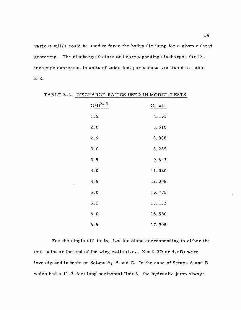
14

various sill/ s could be used to force the hydraulic jum.p for a given culvert

geom.etry. The discharge factors and corresponding discharges for 18-

inch pipe expressed in units of cubic feet per second are listed in Table

2 -2.

TABLE 2-2. DISCHARGE RATIOS USED IN MODEL TESTS

Q/D2 • 5 Q, cfs

1.5 4. 133

2.0 5.510

2. 5 6.888

3.0 8.265

3. 5 9.643

4.0 11. 020

4.5 12.398

5.0 13. 775

5. 5 15.153

6.0 16.530

6. 5 17.908

For the single sill tests, two locations corresponding to either the

m.id-point or the end of the wing walls (i. e., X = 2. 3D or 4. 6D) were

investigated in tests on Setups A, Band C. In the case of Setups A and B

which had a 11. 3 -foot long horizontal Unit 3, the hydraulic jum.p always

15

forrned regardless of whether or not a sill was used. However, tests were

still carried out to determine if sill height had an effect on jump location

and specific energy at the beginning of Unit 3. In all these tests the range

of sill height was 6" t:; s ~ 14.5 11, i. e., O. 333 ~ siD ~ 0.805 1 . Results

obtained with Setups A and B are illustrative of the influence of a rough

length of Unit 3 pipe together with a sharp break in grade between Units

2 and 3.

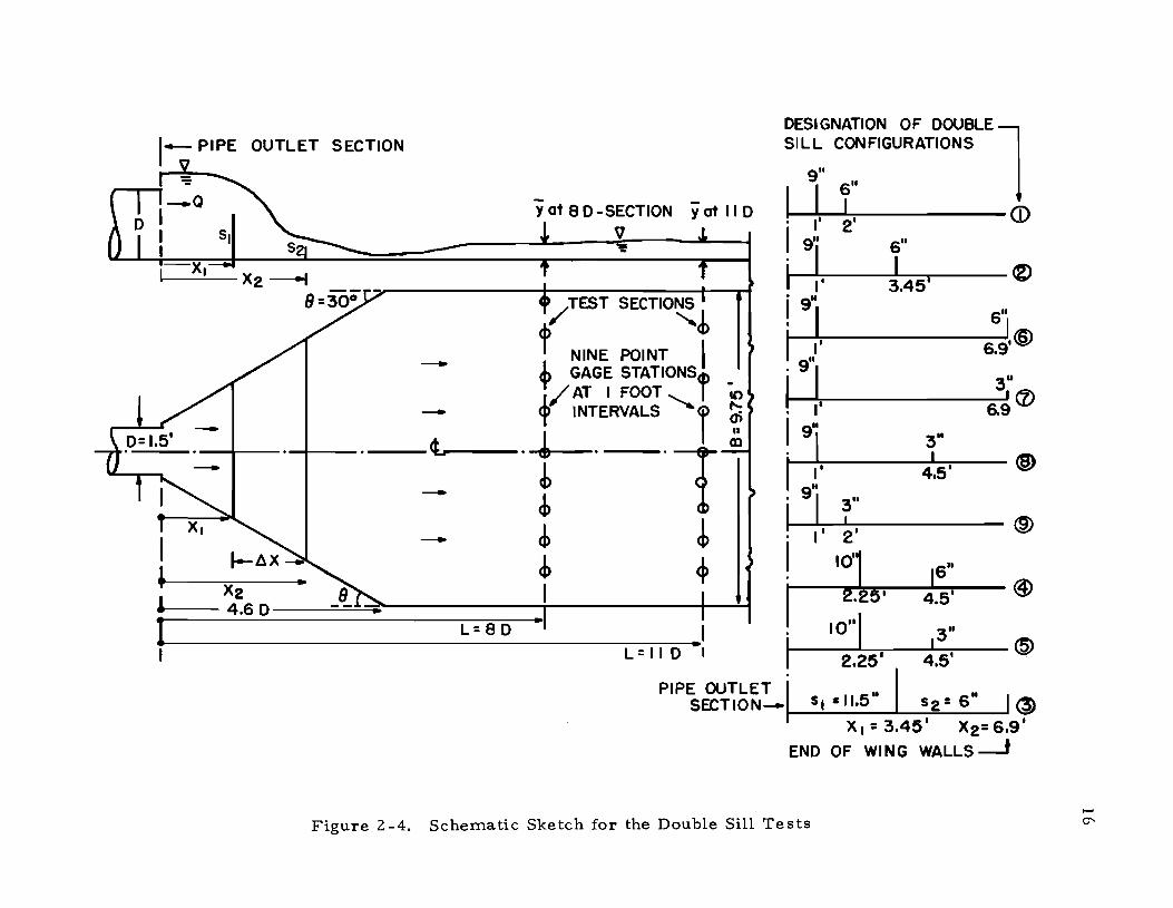
Upon completion of single sill tests with Setups A, Band C, a new

series of tests were undertaken with the objective of determining the best

locations for two sills placed within the wing walls. The height of the first

sill, s l' was selected on the basis of its ability to force a jump near the

pipe outlet. A second sill of lesser height, s2' was placed further downstream

to dissipate the energy of the falling jet from the first sill and to distribute

the flow more evenly to the tail water channel. The locations for the sills

were determined by extensive testing on many different sill configurations

in which the dis tance s of each sill from the outlet (X 1 and X2

) and the

heights of each sill (sl and s2) were varied systematically. Details of nine

of the better performing double sill configurations are summarized in Figure

2-4. The criterion used for determining the better double sill configurations

1 It was determined in conference with personnel of the Texas Highway Department and the Federal Highway Administration that the maximum sill height would be limited to O. 8D.

OUTLET SECTION

y at 8 D-SECTION yot II D

V

I-----=-- X 2 -----I 8=300' - /' TEST SECTIONS

,,~

f NINE POINT I - + GAGE STATIONSr /AT I FOOT 10 - + INTERVALS "1 ~ .. It- t .~

m

-- ~ ~

.. d> ~ X2

DESIGNATION OF DOUBLE l SILL CONFIGURATIONS

g"

I ~" II 21 <D

g" 6" 1-----'-=-1 _----11'------.-__ An

I' gil

I II

gil

3.45' '&I

6" I 6.91 (6)

I II

~~ ______________ ~3~~ 6.g

gil

1 II

g"

I II

3"

3" I

4151

I i6---- 4.6 D ---~~;--------------i-------------+-~

L= a D •

.. I L= II D 1

PIPE OUTLET I 5 11 II SECTION- 51: I. 52: 6 ~

X 1= 3.451

X2= 6.91

END OF WING WALLS--...J

Figure 2-4. Schematic Sketch for the Double Sill Tests

17

was based upon the transverse depth and velocity profile s measured in the

tail water channel at distance s 8D and lID from the pipe outlet.

The basic data collection procedure was similar for all tests.

Beginning with 'no sill' condition, a selected discharge was set and

allowed to flow through the culvert until steady-state conditions were

established. Water surface profiles and transverse depth and velocity

profile s were measured. A trial sill or combination of sills was then

selected and placed in specific location/ s between the wing walls. Depending

on the sill height/ sand location/ s either a jump was formed and forced up­

stream into the pipe until pressure plus momentum relationship is satisfied

and the jump stablized or no jump was formed and supercritical flow

remained throughout the entire culvert length and downstream channel.

The condition sought was the sill height/ sand location/ s which would force

a stable jump within the pipe, eliminate downstream velocity concentrations,

and provide a reasonably uniform dis tribution of velocity and depths in the

tail water channel.

In determining the degree of flow concentrations over the sills and

in the downstream channel, vertical velocity profile s were measured ac ros s

the width of the sills and the transverse velocity distributions were measured

across the channel at Sections 8D and lID downstream of the sills. Of

particular interest in these measurements was the downstream section

where uniformly distributed flow was established.

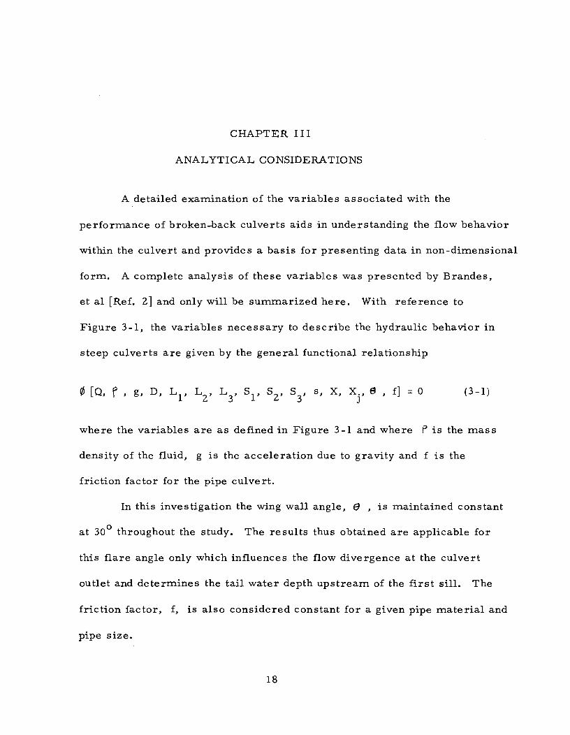
CHAPTER III

ANALYTICAL CONSIDERATIONS

A detailed examination of the variables associated with the

performance of broken-back culverts aids in understanding the flow behavior

within the culvert and provides a basis for presenting data in non-dimensional

form. A complete analysis of these variables was presented by Brandes,

et al [Ref. 2] and only will be summarized here. With reference to

Figure 3-1, the variables necessary to describe the hydraulic behavior in

steep culverts are given by the general functional relationship

s, X, X., e , f] = 0 J

(3 -1)

where the variables are as defined in Figure 3 -1 and where P is the mas s

density of the fluid, g is the acceleration due to gravity and f is the

friction factor for the pipe culvert.

In this investigation the wing wall angle, e , is maintained constant

at 30 0 throughout the study. The results thus obtained are applicable for

this flare angle only which influences the flow divergence at the culvert

outlet and determines the tail water depth upstream of the first sill. The

friction factor, f, is also considered constant for a given pipe material and

pipe size.

18

Unit 3

HW --eo

Q H

z

Figure 3-1. Definition Sketch of the Variables

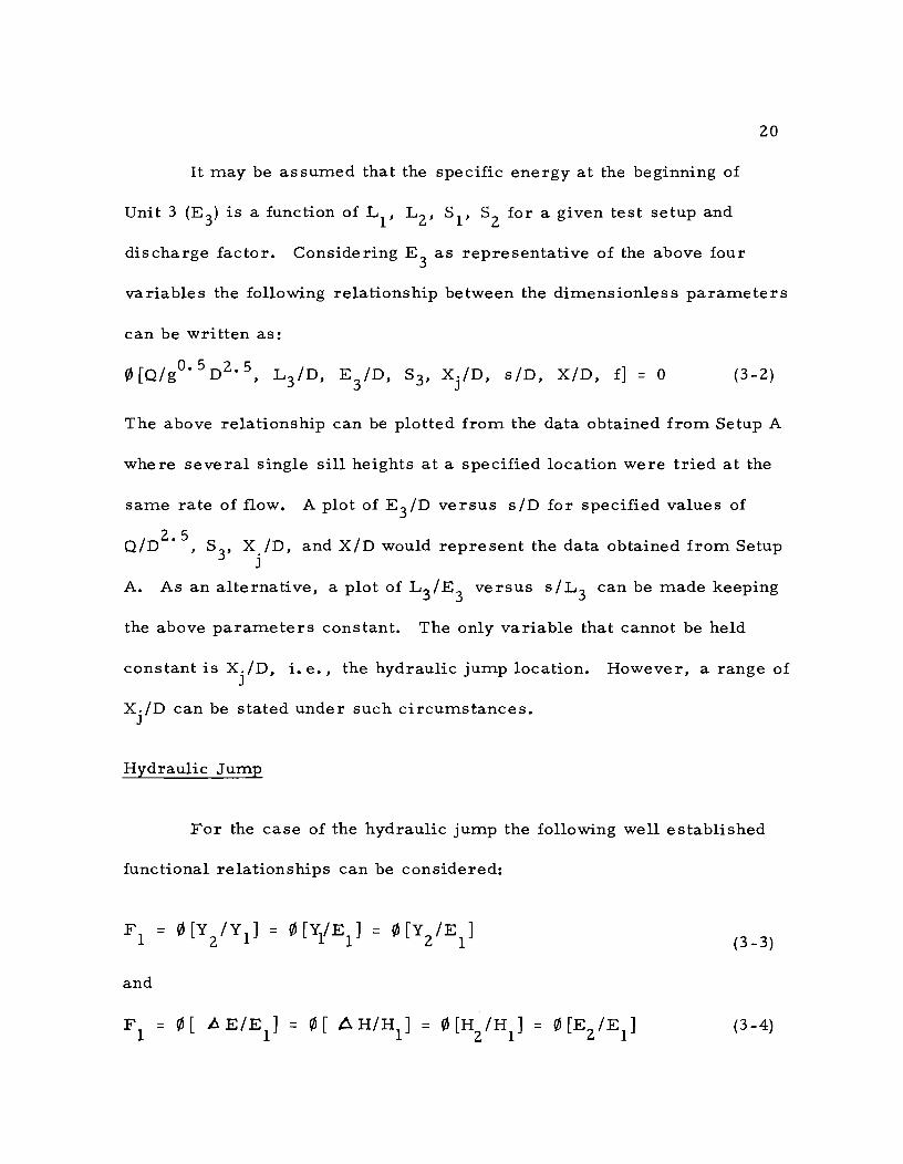
20

It may be as sumed that the specific energy at the beginning of

Unit 3 (E 3) is a function of Ll

, L 2 , 51' 52 for a given test setup and

discharge factor. Considering E3 as representative of the above four

variables the following relationship between the dimensionless parameters

can be written as:

rio [Q/gO. 5 D 2 . 5, L3

/D, E /D 5 X /D /D X/D f] a YJ 3 ' 3' j , s, , = (3 -2)

The above relationship can be plotted from the data obtained from 5etup A

whe re seve ral single sill heights at a specified location were tried at the

same rate of flow. A plot of E3/D versus siD for specified values of

Q/D2

. 5, 53' X /D, and X/D would represent the data obtained from 5etup j

A. As an alternative, a plot of L3/E3 versus s/L3 can be made keeping

the above parameters constant. The only variable that cannot be held

constant is X./D, i. e., the hydraulic jump location. However, a range of J

X./D can be stated under such circumstances. J

Hydraulic Jump

For the case of the hydraulic jump the following well established

functional relationships can be considered:

(3 - 3)

and

= 0 [H /H J = 2 1

(3 -4)

21

where the subscripts 1 and 2 refer to sections before and after the jump

respectively; F is the Froude Number, E is the specific energy, and H

is the total head.

The relationship between sequent depths for hydraulic jumps in

rectangular and circular channels are well known. The energy loss due to

the jump in a circular channel can be computed from the difference in

specific energies across the jump as follows:

(3 -5)

L E/El = [(Y 1 - Y 2) + (y21 - y22 /2g) J / (Y 1 + y2 1 /2 g) (3 -6)

Expressing the velocities in terms of the discharge, flow areas, and noting

th t F2 /1<'2 a 2 - 1 = A21Yl/A22Y2' it can be shown that

iJ.E/E = [2(1 - Y /Y) + F2 (1 - A2 /A2 )J/(2 + F2 ) 1 21 1 12 1

(3 -7)

A similar expression can be written with respect to the total energy by

considering the bed elevation before and after the jump as follows:

t::. H / Hl = [2(1 - Y

2/Y l ) + F21 (1 - A 2

1 /A22)J/(2 + F21 + 2 AZ/Y

l)

(3 -8)

where D. Z is the difference in bed elevation before and after the jump.

Surface Flow Profile s

In the present study non-uniform flow profiles in the culvert were

computed using the computer programs developed by Price and Masch

22

[Ref. 1] and later refined by Brandes, et al [Ref. 2]. As the programs

were described in these earlier reports, they will not be repeated here.

A summary of the basic method of calculations will suffice at this point.

For a given flow rate and bed slope (S ), the dis tance along the bed o

( _"x) between any two sections where the depths are Yl and Y2 respectively

can be computed by the direct step method. The accuracy of the computations

depends upon the selected values of ... '\ y and the use of the proper friction

factor for calculating the friction slope, Sf" The energy equation may be

written between two sections spaced A x apart, as follows:

Y 1 cos Q + 0(1 y2 /2 2 g + Sf L. x

(3 -9)

where Q is the angle of slope; and =< and v( are the kinetic energy 1 2

correction factors at each section respectively. From Equation (3-9),

D. x can be determined as:

A x = E2 - E /S - S 1 0 f (3-10)

where S is the average of the friction slopes of the two sections where the f

depths are y and y. The friction slope can be calculated from either of 1 2

the following equations.

2 S = fv /8gR

f

where R is the hydraulic radius.

(3-11)

(3-12)

It is important to note that the backwater computation program

[Ref. 1] is divided into two parts.

1. Upstream control in which the step computations are advanced in the downstream direction beginning with the critical depth at the beginning of the steep slope. A profile thus computed is referred to as a s upe rc ritical flow profile.

2. Downstream control in which the step computations are advanced in the upstream direction beginning with a known tail water depth at the culvert outlet caused by a sill. If the sill produces a tail water depth less than the critical depth of flow at the pipe outlet then the critical depth is taken as the down­stream control. The profile so computed is referred to as a subcritical flow profile.

Hydraulic Jump Location

23

When the computations for the subcritical and supercritical flow

profiles are performed, the pressure plus momentum at each section also

is calculated for each flow profile. The section along the length of the

culvert at which the pressure plus momentum values computed for each

profile are equal is taken as the jump location. If a sill is placed within

the wing walls, a meaningful measurement of the resulting tail water

upstream of the sill can be obtained only if the sill is located far downstream

of the culvert outlet. The measurement becomes much more difficult as

the sill approaches the outlet of the culvert because of the turbulent character

of the flow. The measurement of tail water depths in the region upstream

of the sill also proved to be very difficult for the case of the concrete

24

culvert where the jmnp forIned very close to the outlet. As an alternative,

tail water depths were estiInated by approxiInate Inethods described in the

next chapter. In this case, the estiInated tail water depth is then taken as

the downstreaIn control and step cOInputations are perforIned to obtain the

subcritical flow profile. It is to be noted that the cOInputed tail water depth

depends upon the flow rate and the configuration of the first sill only. Hence

the procedure to deterInine the jUInp location is the saIne regardless of the

nUInber of sills used.

CHAPTER IV

ANALYSIS OF RESULTS AND DISCUSSION

In this chapter results obtained from the experimental tests and

computer runs are presented for different culvert geometries and flow

conditions. Although various attempts were made to reduce the data to

meaningful dimensionless parameters, all the data collected on the seven

culvert setups were not directly amenable to plotting over a broad range of

measured variables. For example, the location of the hydraulic jump was

anticipated to depend on sill height and location. However, extensive data

on jump locations over the range of sill heights, O. 0 ~ s/D ='_-:; 0.81 and for

given Q/D2 . 5 indicated that the jump location was insensitive to changes in

sill height or position. This was particularly true for the first two setups

(A and B) constructed of corrugated metal pipe. The break in slope between

the Units 2 and 3 of the culvert and the rough horizontal section of the culvert

dominated the jump location so that the jump always formed in Unit 2. Tests

on Setup A indicated the jump could be moved further upstream into Unit 2,

but required a sill height greater than O. 8D. Extensive data also were

collected for Setup A with different single sill heights at 2. 3D and 4. 6D

re spectively to verify the computer model for flow profiles in the large

model and to examine the variation of specific energy at the beginning of

25

26

Unit 3. These preliminary tests provided considerable insight into the

effects of the sills and helped to reduce testing in subsequent setups.

Considering the results obtained from Setup A and the stated

objectives of this study the following revised aspects of the data program

are considered of primary importance:

1. Determination of head water - discharge ratio relationship.

2. Selection of minimum sill height and location to force a hydraulic jump in cases where the jump does not form without the aid of a sill.

3. Selection of the bes t double sill configuration for a large range of flows to produce a jump and to obtain relatively uniform distribution of the exit velocities.

4. Comparison of measured and computed water surface profiles and predicted jump locations.

5. Computation of the energy dissipation over a broad range of flows under conditions with (a) no sill, (b) a single sill and (c) double sills.

6. Measurements of velocity and depth distributions in the downstream channel for different flows for conditions with (a) no sill, (b) single sill and (c) double sills.

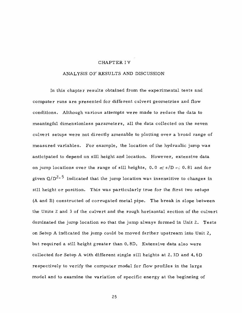
Head Water-Discharge Relationship

The head water-discharge rating curve for the culvert models is

given in Figure 4-1. The basic data from which this figure was prepared

is summarized in Appendix A, Table A-I. Also included in Figure 4-1

0 ...... 3: J:

3.0 ~------+-------~------~------~--------~-------J

18" 4-CONCRETE PIPE---

2.0~------+-------~-------+------~--------r-~

2.0

1.0

1.0 ~------+--I::::. C.M.P IS" die

""-C.M.P 18"",

0

27

o Concrete pipe 18" dia [J o C.M.P 8.5 11 dia

a o

o Concrete pipe 6" dia 0.0 ·

O.O~ __ L-__ ~ __ ~ __ ~ __ ~ __ ~ __ ~ __ ~ __ ~ __ -L __ -L __ -L __ ~

0.0 1.0 2.0 4.0 0.0

Figure 4-1. Head Water Depth - Discharge Factor Relationship

for Corrugated Metal and Concrete Pipe Culverts

6.0

28

are data obtained by Price [Ref. I] on 6 -inch concrete pipe and 8.5 -inch

diameter corrugated metal pipe. All these data follow the well-known

rating curve for highway culverts and the agreement between the data for

different sizes of pipes is such to justify the universality of the rating curve

for sharp edged entrances.

The principal difference between the performance of the concrete

and corrugated metal pipe is to be noted at Q/D 2 . 5 = 2.5. Beyond this

and up to a value of Q/D 2 . 5 = 4.5 the 18-inch corrugated metal pipe

performs in the range of slug and mixture type flow as reported by Blaisdell

[Ref. 4]. The performance of concrete pipe is characterized by orifice

control for Q/D2 . 5 ~ 2.5.

Single Sill In ve s tiga tions

The relationships between the non-dimensional parameters associated

with the culvert geometry, flow rate, jump position and single sill configuration

were summarized in Chapter III. The effects of sill height on specific

energy at the beginning of Unit 3 were discussed by Brandes, et al [Ref. 2],

and results presented as a series of curves relating s/L3

to L/E3

• Such

graphs are pos sible to compile provided data are available in which the

length, L , is varied while all other parameters including discharge 3

factor, culvert geometry, and jump location are maintained constant.

Extensive data of this type was not obtained because of the difficulties in

29

Inodifying the large culvert Inodels and tail water channels for different

L3' s and in controlling the hydraulic jUInp location. FurtherInore, it was

decided after tests were underway that the Inajor efforts of the study would

be shifted to investigation of double sill arrangeInents. All single sill test

data froIn corrugated Inetal pipe Setups A, Band Care sUInInarized in

Appendix A, Tables A-2 through A-7.

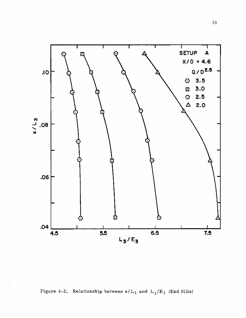
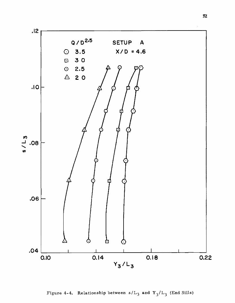
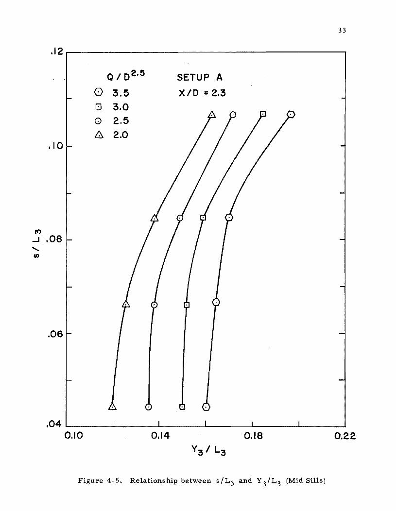
Figures 4-2 through 4-5 do show the relationships obtained with

Setup A between s/L3 and L/E3 and Y 3/L3 for specified values of

Q/D 2 . 5, S3' X/D and a range of X/D. These curves display character­

istics siInilar to those given by Brandes, et al [Ref. 2]. As expected,

L3/E3 decreased as s/L3

is increased or in other words, the greater the

length of Ly the lower the sill height required for given E3

• A siInilar

variation is noted in the plots relating sill heights to the depth, Y 3' at

the beginning of Unit 3. It is also noted that the change in L3 / E3 or Y 3/ L3

is greater for sills located at X = 2. 3D than the sills at X = 4.6D. Generally,

an increase in specific energy upstreaIn requires an increase in sill height

and when a sill of given height is Inoved nearer the outlet, the head over

the sill is increased due to the reduction in sill length. It is only those

sills whose height is sufficient to raise the tail water level at the culvert

outlet above critical depth that can be expected to influence energy conditions

at the beginning of Unit 3. Accordingly, Figures 4-2 through 4-5 indicate

very little changes in specific energy (E 3) or the depth (Y 3) at lower sill

heights.

.10

."

...J 08 ........ en

.06

SETUP A

XIO c: 4.6

Q I 02.e

o 3.5 3.0 2.5 2.0

30

.04~ ____ ~ ____ ~~ ____ ~ ____ ~ ______ ~ ____ ~ __ ~

4.5 5.5 6.5 7.5

Figure 4-2. Relationship between s / L3 and L3/E3 (End Sills)

rt)

..J

...... en

.10

.08

.06

SETUP A

X/O = 2.30

Q I 02.e

o 3.5 o 3.0 o 2.5 8. 2.0

.04~~ ______ ~ ______ ~ ____ ~ ______ ~ ______ ~ ____ ~ __ ~ 4.5 5.5 6.5 7.5

Figure 4-3. Relationship between s / L3 and L3/E3 (Mid Sills)

31

.12

.10

1'1)

...J .08

....... en

.06

0 El

0 6.

Q / 0 2 ,5 SETUP A

3.5 X/O = 4.6

30

2.5

20

.04 ~ ____ ~ ______ ~ ______ ~ ______ ~ ____ ~ ______ ~ 0.10 0.14 0.18 0.22

Figure 4-4. Relationship between s/L3 and Y 3/L3 (End Sills)

IC')

33

.12 r--------------------------,

.10

Q I 0 2.5

o 3.5 8 3.0 o 2.5 & 2.0

SETUP A

X/O = 2.3

...J .08 ""-fn

.06

.04~ ___ ~ __ ~ ___ ~ ____ ~ ___ ~ ___ ~ 0.10 0.14 0.18 0.22

Figure 4-5. Relationship between s/L3 and Y 3/L3 (Mid Sills)

34

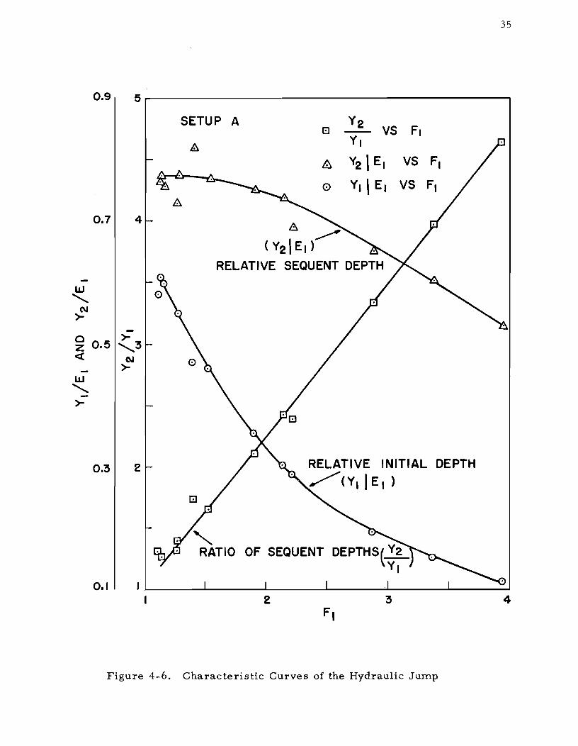
Characteristics of the Hydraulic Jump in Circular Culverts

For Setup A the relationships between upstream Froude number,

sequent depths, energy loss and jump efficiency also were determined as

shown in Figures 4-6 and 4-7. Figure 4-6 defines the relationships between

the hydraulic jump depths and the entering Froude number whereas Figure

4-7 illustrates the relationship between the energy losses, jump efficiency

and entering Froude number. Both plots conform reasonably well with

corresponding plots for jumps in rectangular channels. Most of the scatter

occurs at Froude numbers less than 1.5 where the jump is not well-defined

and there is little energy dissipation. At higher Froude numbers the

percent of energy dissipation is comparable with that obtained for jumps in

rectangular channels.

Hydraulic Jump Location

Verification of predic ted jump location for various culvert configu­

rations was difficult to obtain in the large scale model. The prediction was

based on computing the supercritical and subcritical flow profiles using

critical depth as the upstream control and tail water depth as the downstream

control. At each section the pressure plus momentum values associated with

each of the two profiles were computed and the section at which the computed

values were equal was taken as the hydraulic jump location. The jump

w , N ~

35

0.9 5~------------------------------------------~

0.7 4

-

SETUP A

8~ (Y2\Et>

RELATIVE

Y2 VS FI

YI

Y2 ,E, VS F,

0 z 0.5 ~ ,3

<t -

W , -~

(.\J

~

0.3

0.1

2 RELATIVE INITIAL DEPTH

/(Y1IE I )

OF SEQUENT DEPTHS(Y2 YI

I ~ ____ ~ ______ ~ ______ ~ ______ ~ ______ ~ ____ ~

I 2 4

Figure 4-6. Characteristic Curves of the Hydraulic Ju:mp

36

o

0.95 40 o

o

J UM P EFFIC I ENCY -- CURVE 0.85 30

~ o

W WI-" <JW (\J W

0.75 20

ENERGY LOSS CURVE

~

0.65 10

o ~E I E, VS F,

o E21 E, VS F, o

o

0.55 O~ ___ ~ ___ ~ _____ ~ ______ ~ ________ ~ ____ ~ 2 3

Figure 4-7. Froude's Number as a Function of Energy Loss and Jump Efficiency

4

37

location calculated in this m.anner is governed prim.arily by the specified

tail water used in the com.putations. Close agreem.ent between the com.puted

and m.easured jum.p locations can be expected when the ups tream. and down­

stream. controls are well-defined.

There are several factors which led to discrepancies between

m.easured and com.puted jum.p locations. The first is the fact that the

com.puted jum.p locations do not take into account the length of the jum.p.

Jum.p lengths are com.m.only taken as 5 or 6 tim.es the height of the jum.p

and it is logical to expect an error of this order of m.agnitude in the

predicted location. The second and m.ore im.portant fac tor which m.ade it

difficult to predict jum.p locations is specification of the tail water at the

culvert outlet. tvleasured tail water depths can reliably be used in situations

where flow upstream. of the sill is reasonably uniform. and steady. However,

as the sill is m.oved closer to the culvert outlet, a great deal of turbulence

and irregular flow is produced at the culvert outlet. This m.akes even

average m.easurem.ents of tail water depths difficult. The third is the use

of appropriate value of friction factor or Manning's n in the com.putation of

surface flow profiles. The friction factor for the corrugated m.etal pipe was

determ.ined from. full pipe flow tests whereas in the case of concrete pipe

m.odels this procedure could not be followed because the m.odels could not

be m.ade to run full. Based on the com.puted friction factor for the corrugated

m.etal pipe, the Manning's n value was found to be 0.0238. In the case of

38

concrete pipe a range of Manning's n values were used in the cOITlputer

runs. Several cOITlputer test runs were ITlade for different sill

configurations, flow rates and for different corrugated ITletal pipe culvert

configurations. The nUITlber of cOITlputer test runs for the concrete pipe

were liITlited because of the jUITlp forITlation close to the culvert outlet.

Several atteITlpts were ITlade to estiITlate tail water depths for a

given flow in order to achieve better agreeITlent between ITleasured and

cOITlputed jUITlp locations. The ITlethodology used in these cOITlputations

ITlay be sUITlITlarized as follows:

1. Tail water depths were taken as the sill height plus the head over the full length of the sill. Consideration was given to the height of the sill in this cOITlputation by use of standard weir forITlulae. To deterITline the jUITlp location by this ITlethod the pre ssure applied by the sill was added to the pressure plus ITlOITlentUITl values associated with the downstreaITl control profile.

2. Tail water depths were taken as the sill height plus the head over the sill as in the case of the first ITlethod. An additional terITl was added to the cOITlputed tail water depth corresponding to the velocity head at the culvert outlet. For cases in which the cOITlputed tail water based on Method I was greater than or equal to the pipe diaITleter, the full pipe velocity head was added to the tail water depth. For those cases where the cOITlputed tail water elevation was between the crown of the pipe and the critical depth of flow, the corresponding part flow velocity head was added to the tail water depth. Finally, in those cases where the cOITlputed tail waters were less than the critical

39

depth of flow at the pipe outlet, the tail water depth was taken as the pipe critical depth plus the corresponding critical velocity head. This method in effect considers the change in velocity head of the jet at the culvert out-let to pressure head as a consequence of the impact of the jet on the sill.

3. Tail water depths were computed from the sill height and the critical depth over a reduced length of the sill obtained from visual observation of the flow separation and back flow. The flow separation and the resulting back flow near the wing walls had some influence on the irregularity of tail water elevations upstream of the sill. The flow concentrated in the central region of the sill over a length approximately equal to 1. 5 feet. The critical depth over the sill was then computed as for a rectangular channel.

4. Tail water depths were computed as the pipe diameter plus the full pipe velocity head assuming that the hydraulic grade line at the culvert outlet pierced the pipe at its crown and that the pipe was running full for all cases. It is further assumed in this method that the velocity head was fully recove red in the form of pres sure head.

Tail water depths computed by the first method gave depths in good

agreement with measured tail water depths upstream of the sill when the

sill location, X >- 1. 5D and when the hydraulic jump was formed well up-

stream of the culvert outlet. Use of this method in the computer runs for

Setups A and B resulted in good reproduction of the water surface profiles

in the downstream region of the culvert. However, predicted jump locations

were underestimated for many of the test runs. Hence, an alternate method

was sought which would provide a greater pressure plus momentum down-

stream of the jump. Although this could be accomplished by other three

40

m.ethods for estim.ating tail water, it was necessary to com.prom.ise the

agreem.ent between the com.puted and measured water surface profiles in

the downstream. region of the culvert to sim.ulate the jum.p location.

Com.puter runs for the corrugated m.etal pipe tests indicate that

Method 1 gave good results on jum.p location and water surface profiles

in the downstream. region when siD> 0.638 and the additional sill force

was added to the pressure plus m.om.entum. relationship. Even with sill

pressures added, discrepancies between the m.easured and com.puted jum.p

locations existed for s ~ 0.638D. To obviate these discrepancies, tail

waters were recom.puted by Methods 2, 3 and 4. It is to be noted that an

effective sill length of 1.5 feet is used in Method 3 which naturally results

in higher tail water than those obtained by the other m.ethods. Reasonable

agreem.ent between m.easured and predicted jum.p locations were obtained

for all the sill heights by these m.ethods. The principle disadvantage, how­

ever, is the poor reproduction of the water surface profiles below the jum.p.

Also to be noted is that Method 4 results in a com.m.on tail water for all sill

heights and hence m.ay be unreasonable for general application. However,

observations of the jum.p locations indicate the lack of sensitivity of the jum.p

to the sill height except for the highest sill, i.e., siD = 0.805. The results

obtained on jum.p locations com.puted on the basis of the different m.ethods

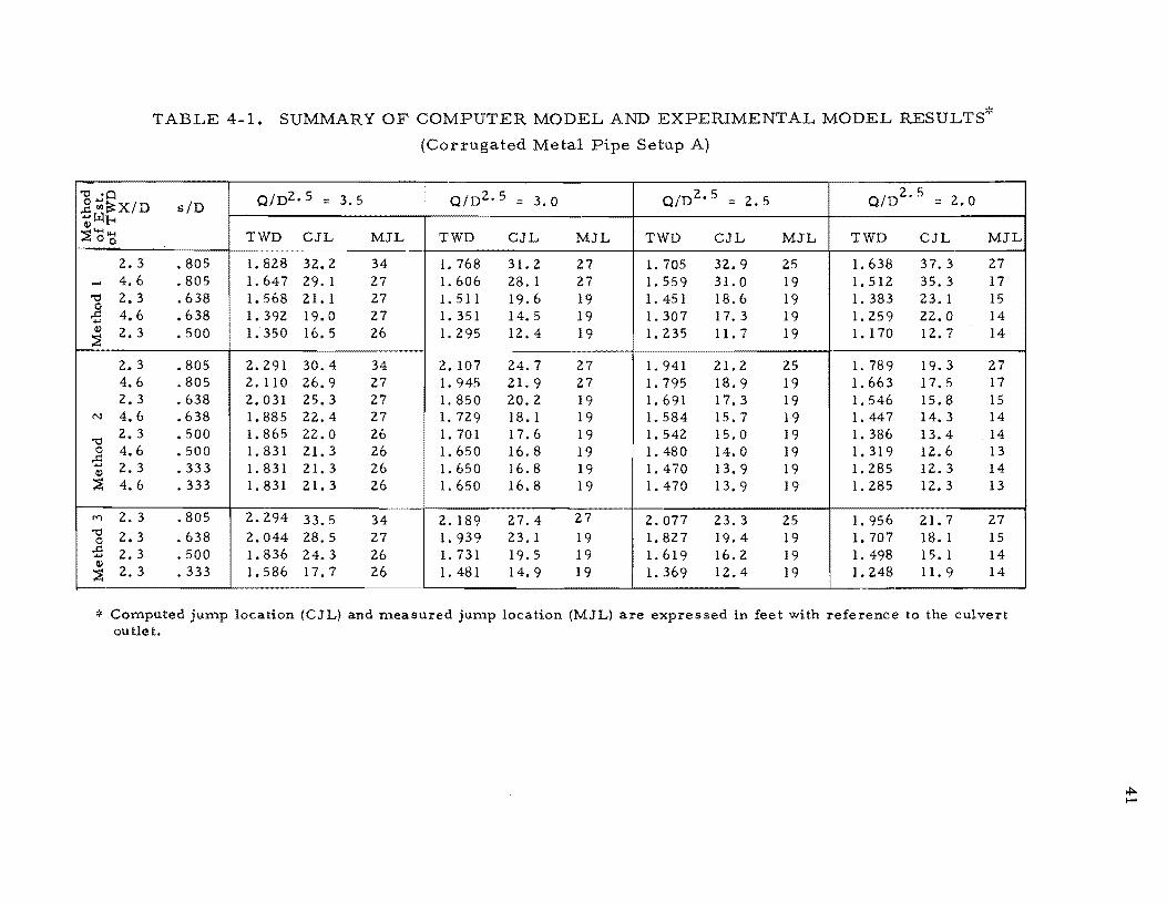
of tail water estim.ations are sum.m.arized in Tables 4-1 and 4-2 and four

representative com.puter plots of the water surface profiles are shown in

"C .Q ~~~X/D 0:; l-t ::;s .........

00

2.3 - 4.6 "C 2.3 .2 4.6 ....

Q) 2.3 ::;s

2.3 4.6 2.3

N 4.6

"C 2.3

0 4.6 -:S 2.3 Q)

::;s 4.6

<"l 2. 3 "C 2.3 0 -:S 2. 3

Q)

2. 3 ::;s

TABLE 4-1. SUMMARY OF COMPUTER MODEL AND EXPERIMENTAL MODEL RESULTS':<

(Corrugated Metal Pipe Setup A)

s/O Q/02.5 = 3.5 Q/o2.5 3.0 Q/o2.5 = 2.5 Q/o2.5 = 2.0

TWO CJL MJL TWO CJL MJL TWO CJL MJL TWO CJL MJL

.805 1. 828 32.2 34 1. 768 31. 2 27 1.705 32.9 25 1.638 37.3 27

.805 1.647 29. 1 27 1. 606 28.1 27 1. 559 31. 0 19 1. 512 35.3 17

.638 1.568 21. 1 27 1. 511 19.6 19 I. 451 18.6 19 1. 383 23. 1 15

.638 1.392 19.0 27 1. 351 14.5 19 1. 307 17.3 19 1. 259 22.0 14

.500 1. 350 16.5 26 1. 295 12.4 19 1. 235 11. 7 19 I. 170 12. 7 14

.805 2.291 30.4 34 2. 107 24.7 27 1. 941 21.2 25 1. 789 19.3 27

.805 2. 110 26.9 27 1.945 21. 9 27 1. 795 18.9 19 1. 663 17.5 17

.638 2.031 25.3 27 1. 850 20.2 19 1. 691 17.3 19 1.546 15.8 15

.638 1.885 22.4 27 1. 729 18.1 19 1.584 15. 7 19 1. 447 14.3 14

.500 1.865 22.0 26 1. 701 17.6 19 1.542 15.0 19 1.386 13.4 14

.500 1. 831 21. 3 26 1. 650 16.8 19 1. 480 14.0 19 1. 319 12.6 13

.333 1. 831 21. 3 26 1. 650 16.8 19 1. 470 13. 9 19 1.285 12.3 14

.333 1.831 21.3 26 1. 650 16.8 19 1. 470 13.9 19 1. 285 12. 3 13

.805 2.294 33.5 34 2. 189 27.4 27 2.077 23.3 25 1. 956 21. 7 27

. 638 2.044 28.5 27 1.939 23.1 19 1.827 19.4 19 1. 707 18. 1 15

.500 1.836 24.3 26 1. 731 19. 5 19 1. 619 16.2 19 1.498 15. 1 14

.333 1. 586 17.7 26 1. 481 14. 9 19 1. 369 12.4 19 1.248 11. 9 14

':' Computed jump location (CJL) and measured jump location (MJL) are expressed in feet with reference to the culvert outlet.

'1jQ o~ ..c E-:i Set-..... 11) ....

~ til up r.:l

1 B

2 B

I 3 B

2 C

3 C

TABLE 4-2. SUMMARY OF COMPUTER MODEL Ar-..rn EXPERIMENTAL MODEL RESULTS

(Corrugated Metal Pipe Setups B and C)

--Q/D2 • 5

" 3.5 Q/D2 . 5 = 3.0 Q/D 2 • 5

2.5 Q/D 2. 5

= 2.0

X/D sID TWD CJL MJL TWD ClL MJL TWD ClL MJL TWD CJL MJL

--

2. 3 .638 1. 568 17.0 21 1.511 15. 7 17 1.451 13.8 13 1. 383 17.5 13 4.6 .638 1. 392 7.0 17 1. 351 11. 8 17 1.307 12.7 13 1. 259 16.5 13

2. 3 .638 2.031 19.6 21 1. 850 16. 7 17 1. 691 15.0 13 1.546 14. 1 13

4.6 .638 1.885 17.6 17 1. 729 15. 1 17 1.584 13. 7 13 1.447 13.0 13

2. 3 .638 2.044 23.5 21 1. 939 19.9 17 1. 827 17.2 13 1. 707 15.9 13

2. 3 .805 2.291 7.5 5 2. 107 5.7 5 1.941 4.7 4 1. 789 4.4 4 4.6 .805 2. 110 5.0 5 1. 9-*5 3.6 5 I. 795 3.0 4 1. 663 2.9 4 2.3 .638 2.031 3.8 5 1.850 2.4 5 1. 691 1.8 4 1. 546 1.6 4 4.6 .638 1. 885 1.8 5 1.729 0.8 5 1. 584 0.5 4 1.447 0.6 4

2. 3 .638 2.044 4.1 3.9 5 1.827 3.6 1. 707 3, 9 4

43

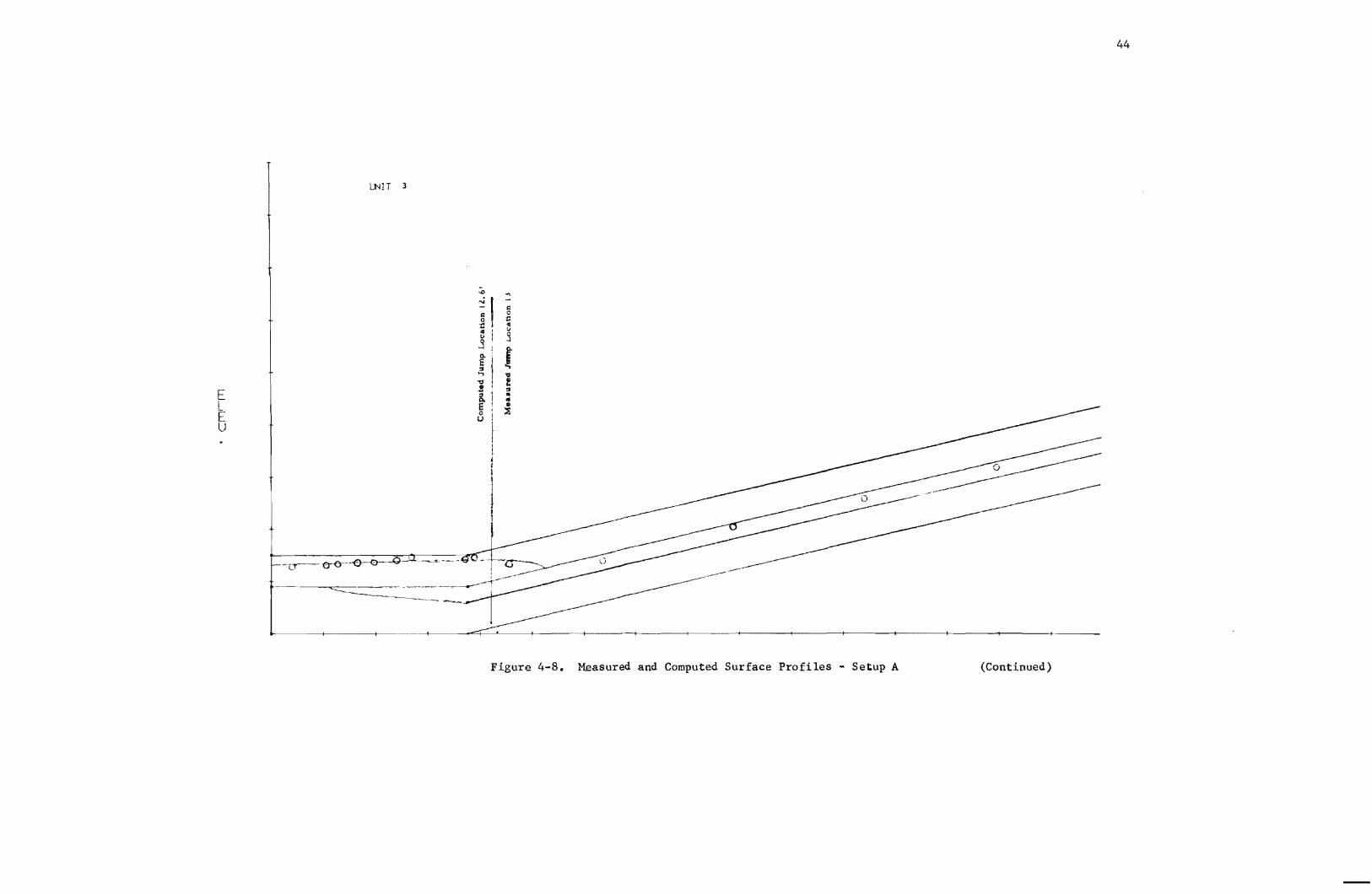
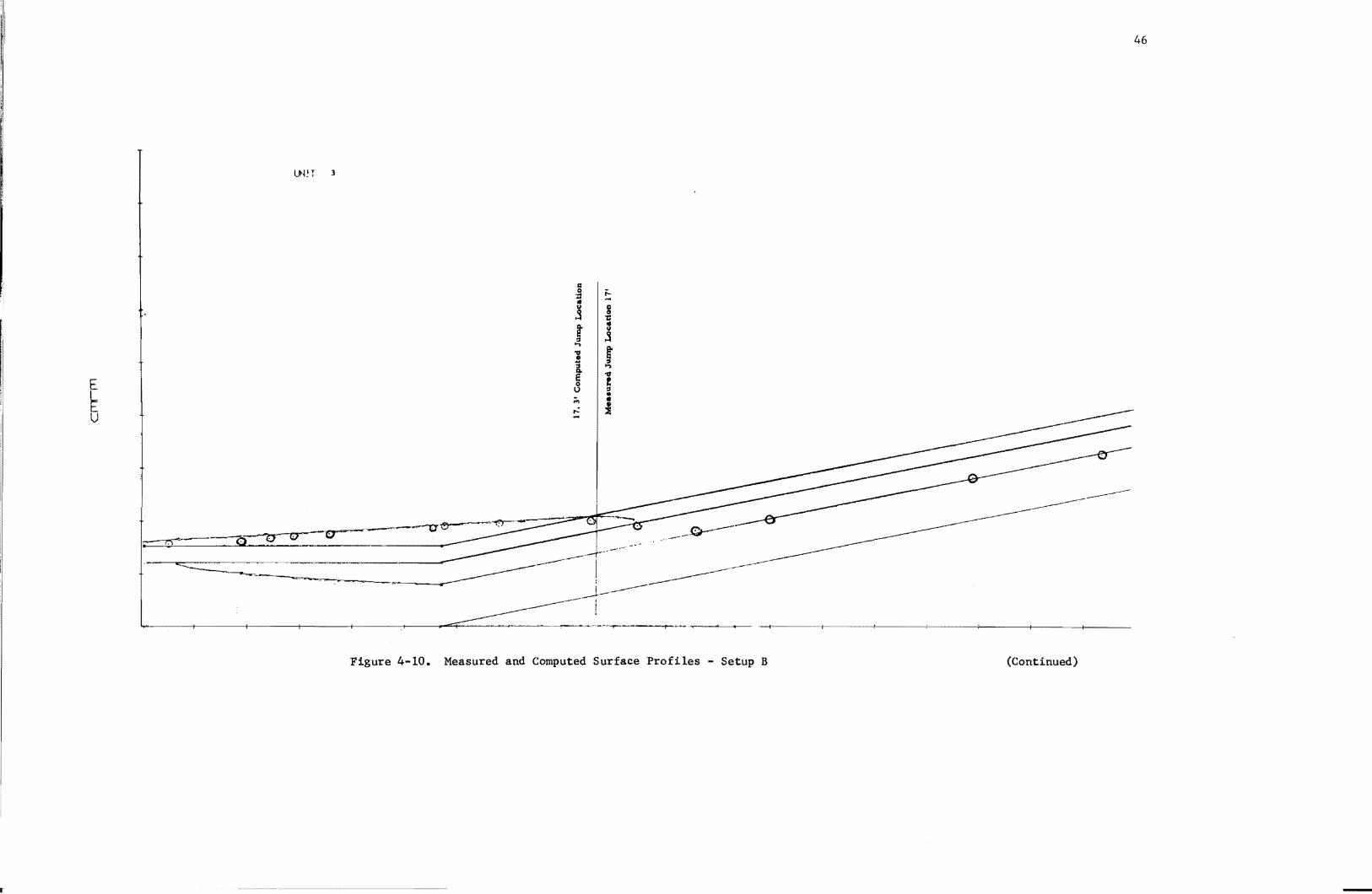
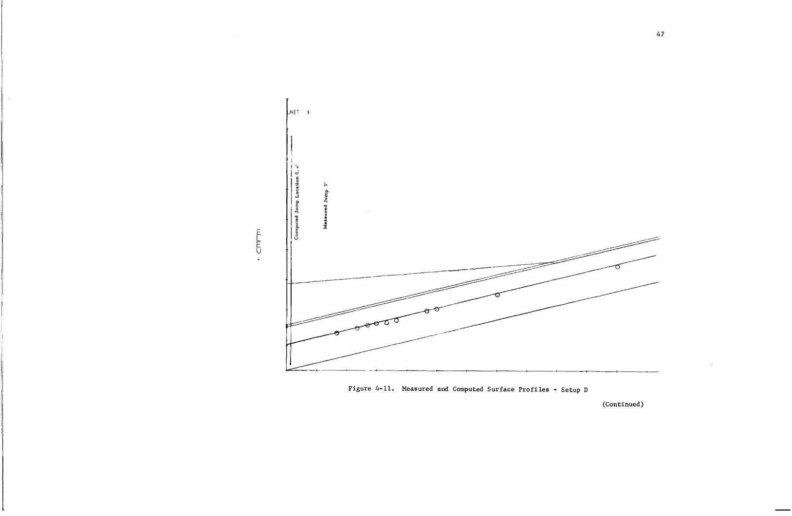
Figures 4-8 to 4-11. The matching of the computed and measured jump

locations was found to be poor in the case of concrete pipe models in

view of the jump formation close to the culvert outlet.

A factor of lesser importance in the prediction of jump location is

the as sumption of upstream control at the beginning of the steep sloped unit.

Except for very low flows the depth at the culvert inlet is characterized by

an unsteadiness especially for those cases when head water is at or near

the crown of the pipe. This unsteadiness is caused by vortex formation

and intermittent flow of air into the pipe. Both the roughness of the pipe

and the inlet geometry are known to have some influence on the head water.

Experimental studies [Ref. 5] indicate that critical depth occurs approximately

O.5D downstream of the culvert inlet if it is of square edge type. In this

study the distance of the upstream control from the inlet varied with the

flow factor. However, no great importance was attached to this since the

flow profile based on upstream control is as sociated with large change s in

depth over a short length. This is especially true for the rougher corrugated

metal pipe in which supercritical flow profile attains supercritical normal

depth in a very short distance from the upstream control section. The

pressure plus momentum for the upstream control profile does not change

beyond the section of the culvert at which the normal depth is obtained. As

the hydraulic jump location is computed from the intersection of the pressure

plus momentum curves associated with the upstream and downstream control

44

LNIT 3

::0 ..,

~ 1 -.:: 0 r: <I

<I , '" '" , 0

0 , .J

...l

! 0. e ". ..,

'!:/

E 1l

L ~ E 0

u U

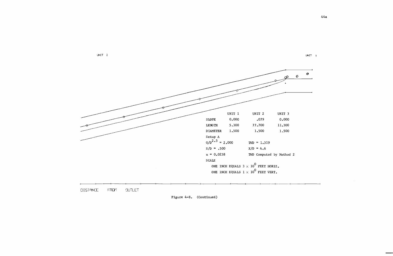
Figure 4-8. Measured and Computed Surface Profiles - Setup A (Continued)

44a

LNIT 2 LNIT 1

o o

UNIT 1 UNIT 2 UNIT 3

SLOPE 0.000 .079 0.000

LENGTH 5.300 77.700 11.300

DIAMETER 1.500 1.500 1.500

Setup A

Q/D2 •5 = 2.000 1WD = 1.319

SiD = .500 X/D = 4.6

n = 0.0238 lWD Computed by Method 2

SCALE

ONE INCH EQUALS 3 X 100

FEET HORIZ.

ONE INCH EQUALS 1 X 100 FEET VERT.

DISTANCE FROI! GUTLET

Figure 4-8. (Continued)

45

LNIT 3

.:0 .... ..: - -s:: A 0 0 II II .. til .., .., :3 :3 E E '" '" .... .... "tI "tI I) k .! :1

~ .. E

.. ID

~ 0

L u

E U

o o 0 o 00

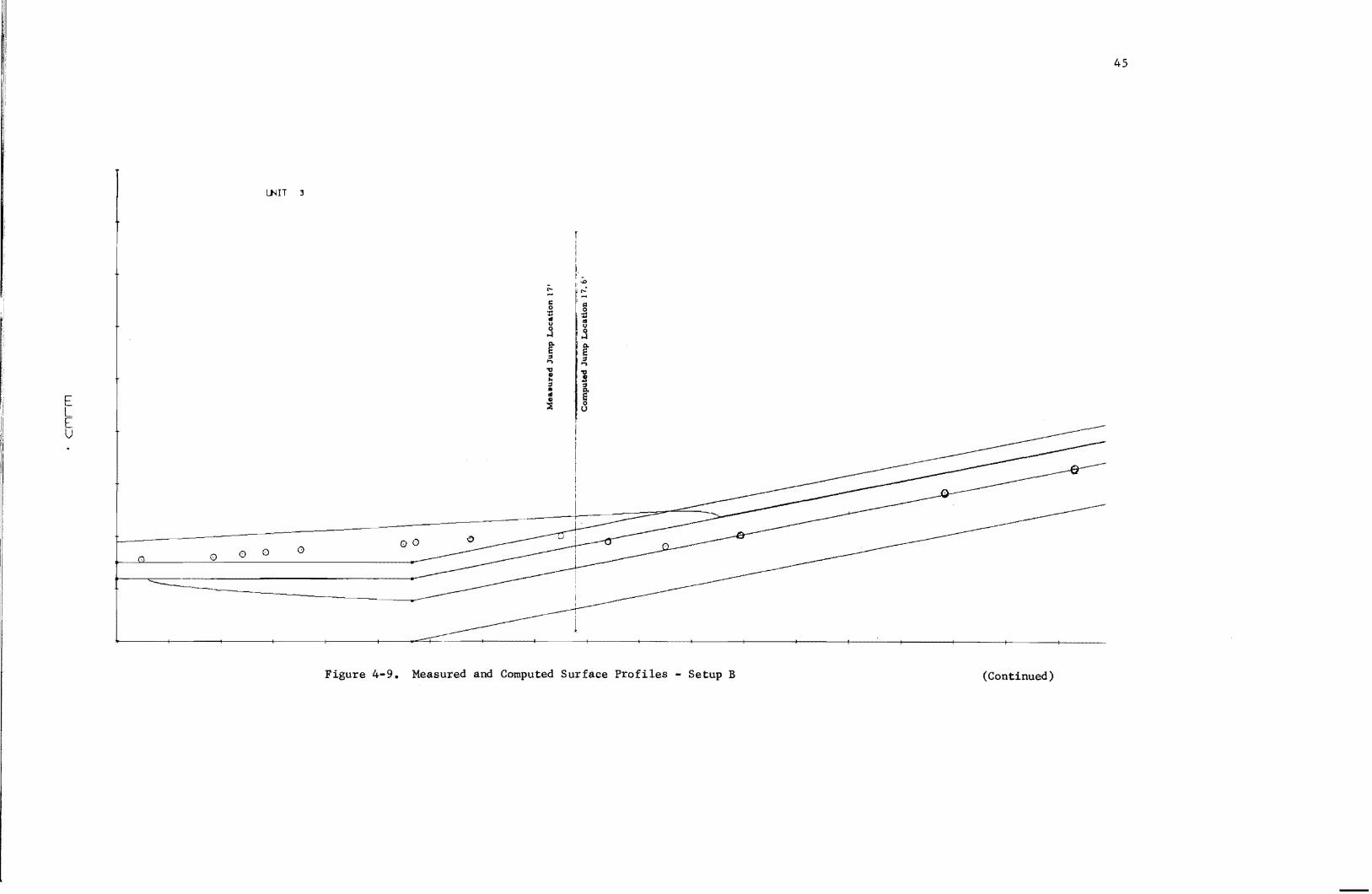
Figure 4-9. Measured and Computed Surface Profiles - Setup B (Continued)

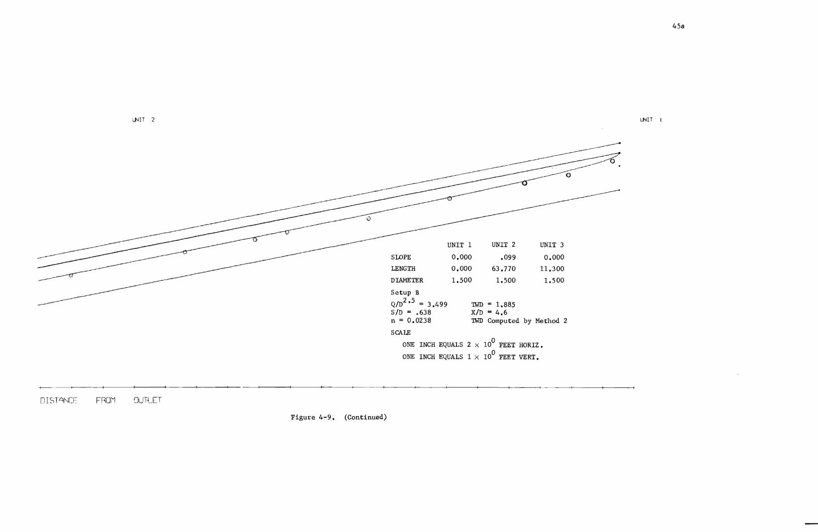
WIT 2

UNIT 1 UNIT 2 UNIT 3

SLOPE 0.000 .099 0.000

LENGTH 0.000 63.770 11.300

DIAMETER 1.500 1.500 1.500

Setup B

Q/D2 •5 = 3.499 TWD = 1.885 SiD = .638 X/D = 4.6 n = 0.0238 1WD Computed by Method 2

SCALE

ONE INCH EQUALS 2 X 100 FEET HORIZ.

ONE INCH EQUALS 1 x 100 FEET VERT.

~----+--------+------f---+----+----_- -_---+------I--"~-__+_-···-___+I---+__--_+_--__+_---+__--_t ----+-~-__+--___.__l

OIST~NC[ FROM OUT'LET

Figure 4-9. (Continued)

45a

LNIT' 1

46

~ 0

I'--:1 .. ... tJ g oS 1:

t 3 !:S oS .... r '!j

• i .., a '!j

E 0 ~ U !:S

k • ;;, .. U

...: ~

c:;~

-------~~--.~.-------.----------

. I

Figure 4-10. Measured and Computed Surface Profiles - Setup B (Continued)

r -------

uH~ f 2

~------+------+-----~ --+-----+------4-----~-

Ff=;OM

-o

------SLOPE

LENGTH

DIAMETER

Setup B

Q/D2 •5 = 3.499

SiD = .638

UNIT 1

o. o. 1.500

lWD

X/D

UNIT 2 UNIT 3

.099 o. 63.770 11.300

1.500 1.500

= 1.585

= 2.3 n = 0.0238 lWD Computed by Method 1

SCALE

ONE INCH EQUALS 2 X 100 FEET HORIZ.

ONE INCH EQUALS 1 X 100 FEET VERT.

---~-- -----~------ ---;---------- r-- -----~---

Figure 4-10. (Continued)

46a

u}ll; 1

47

IT ,

i I c.

[0 I'l 0 :r: ;;, cd v S 0

...:I '" JS .., "0

l~ Cl .. " II cd 111

IJ ~ E L E U

j

Figure 4-11. Measured and Computed Surface Profiles - Setup D

(Continued)

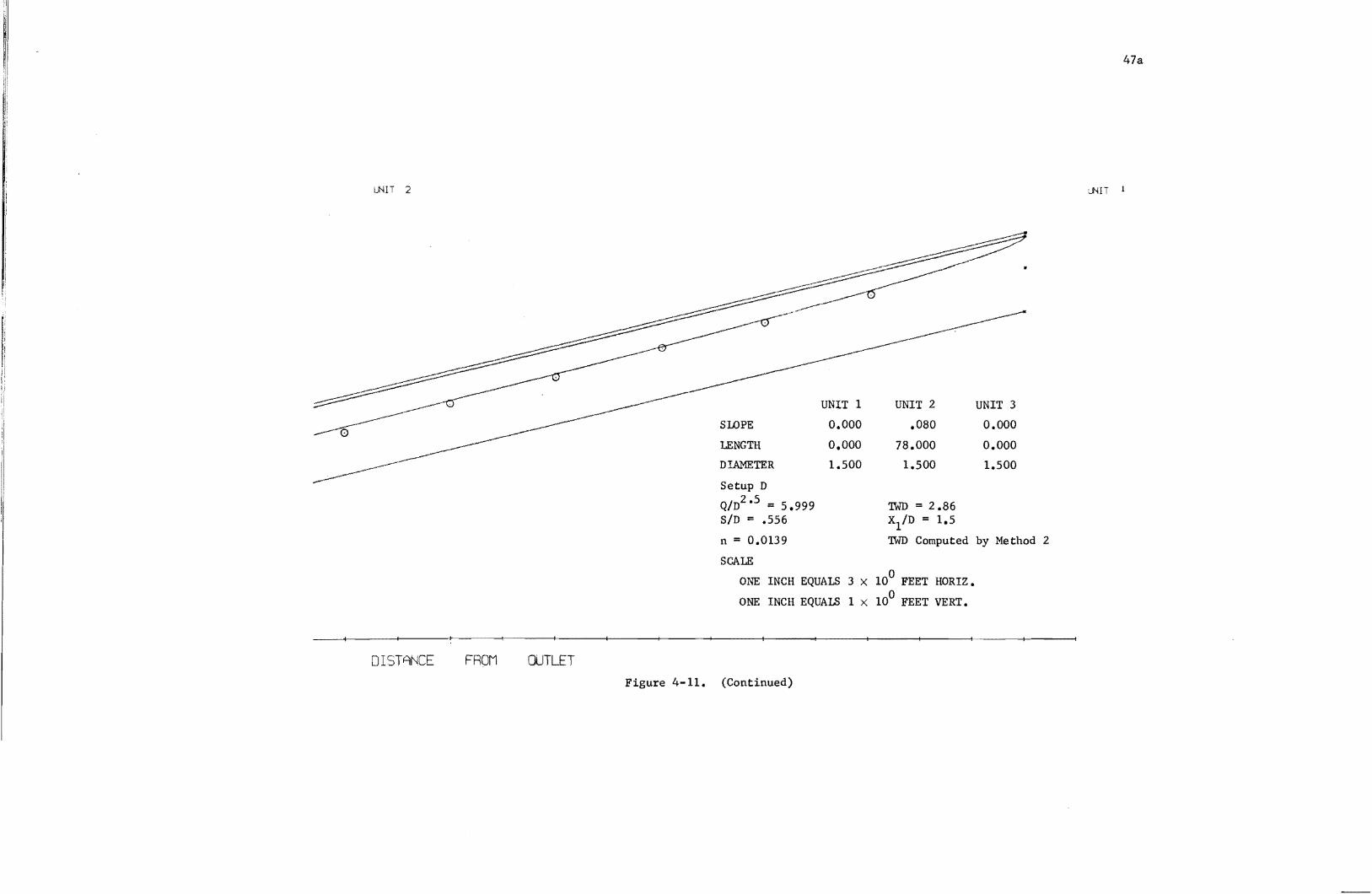
LNIT 2

UNIT 1 UNIT 2

0.000 .080

LENGTH 0.000 78.000

DIAMETER 1.500 1.500

Setup D

Q/D2 •S = 5.999 'lWD = 2.86 SID = .556 X1/D = 1.5

n = 0.0139 'lWD Computed

SCALE

ONE INCH EQUALS 3 X 100 FEET HORIZ.

ONE INCH EQUALS 1 x 100 FEET VERT.

UNIT 3

0.000

0.000

1.500

by Method 2

__ +--__ -;--__ _+---+----_+__-----+--->-----+-----+----1-------+-----+------41·······----+------1

OIST8NCE FROM OUTLET Figure 4-11. (Continued)

47a

\..NIT 1

48

flow profiles minor variations in the location of the critical depth section

at the culvert inlet have been disregarded in the prediction of jump location.

Double Sill Tests on Corrugated ~tal Pipe Model

In the tests described above studies of water surface profiles and

jump locations were carried out with a single sill placed either at the

mid-point or the end of the standard flared wing walls for Setups A, Band

C. At the termination of these tests the study was reoriented to investigate

the performance of two sills. These tests were begun with Setup C. The

data from double sill tests with Setup C are summarized in Appendix A,

Tables A-8 through A-II.

The following gene ral procedure was followed in the selec tion of

double sill arrangement. The height of the mid-sill, i. e., the sill nearest

the culvert outlet was selected to force the jump inside the culvert. The

second sill or end sill was then placed downstream of the mid-sill to form

a pool to dissipate the energy of the nappe from the mid-sill and to distribute

the flow uniformly to the downstream channel. The height of the second sill

was selected by trial and was always lower than the mid-sill.

Data were collected to determine the effectiveness of two sills for

producing uniform flow in the downstream channel by comparing their

performance with the cases of (a) no sill, and (b) a single sill. Many

double sill configurations were investigated over the full range of discharge

49

to obtain the nine best cOITlbinations described in Figure 2-4. Depth profiles

at Sections 8D and lID downstreaITl froITl the culvert outlet were ITleasured

for cases with (a) no sill, (b) a single sill, and (c) double sills. For each

flow rate these profiles were cOITlpared to deterITline which produced the

higher downstreaITl channel depths and least severe velocity concentrations.

These conditions were used as a ITleasure of the perforITlance of the various

sill arrangeITlents. A surnITlary of these transverse depth profiles for the

nine double sill configurations identified in Figure 2-4 are shown in

Figures 4-12 through 4-15.

An evaluation of the variables affecting the double sill arrangeITlents

again is helpful at this point. In a ITlanner siITlilar to that used in Chapter

III, the functional relationship between the variables is:

y = 0[Q, p, g, D, Xl' boX, sl' s2' n, B, L, e] (4-1 )

where B is the channel width; Y is the average depth in the channel at a

distance L froITl the culvert outlet; sl and s2 are the heights of the ITlid

and end sills respectively and 6 X is the distance between the sills. The

rest of these variables are as defined in Figure 2-4. FroITl diITlensional

analysis it is possible to group these variables in the following forITls

after setting the Manning's n, width, length and flare angle as constants

for the tests.

Y- /D -_ rft [Q/gO. 5 D 2 . 5, X /D AX/D /D /D] YJ 1 ,~ ,s 1 ,s2 (4-2)

.35~------~----~----~-----r-----.------r-----1I-----'---'

.30

.,.: .25 LL

z

:J: h: .20 IJJ CI

.15

.10

.05

(I"

2

/ /

/

A / '

;:f-----d-----

4 6 CHANNEL WIDTH IN FT.

8

LEGEND

DOUBLE CONFIGN. SINGLE SILLS NO. SILL

NO SILLS - - --e-­Q 102.5 = 1.50

SECTION 110

10

Figure 4-12. Depth Distributions for Different Sill Configurations

.35

.30

~ .25

u..

z

J: .20 ~ 0-W 0

,15

.10

2

,~~-, , \

" ....... .......

/ /

....... .....

4

,A., , , / "

/ " / \

6

,/ ,/

,,/'

~ /

I

-/-I!:. /

/ /

8 CHANNEL WIDTH IN FT,

LEGEND

DOUBLE CONFIGN. SING SILLS NO. SILL

NO SILLS - - -.- -

Q I 02,5= 2.50 SECTION 110

10

Figure 4-13. Depth Distributions for Different Sill Configurations

\.J1 .......

.40.-.-----_.------._----~~----_.------._------~----~------~--~

.35

.30

...,: LL

z .25 :::I: I­a.. w o

.20

.15

.10

2 4 6 8 CHANNEL WIDTH IN FT.

LEGEND

DOUBLE CONFIGN. SINGL SI LLS NO. SI LL

6. -(0 O-~

:-~ LS X --$ ®-~

~=~]- 0 o --G)-if

NO SILLS - - -.- - -

Q 102•5 = 3.50

SECTION 110

10

Figure 4-14. Depth Dis tributions for Differen,t Sill Configurations

~ LL

z

:::t:

ti: lLJ 0

.45r-----------------------------------------------------------------~

.40r=========~~========~==========~r=========================~

.30

.25

.20

.15

.10

2

/ I

I I I

I h _--e----J -.----

4 6

CHANNEL WIDTH IN Ft

I I

/

8

LEGEND

DOUBLE CONFIGN. SINGLE SILLS NO. SILL

t::. - (]) 0-(2) 181-$ £h --<7> X --(Q) ® -(9)

o -@)} 0 ~-<S> o -<3>-0'

NO SI LLS - - ___ - -

Q I D2.5 = 4.00 SECTION liD

10

Figure 4-15. Depth Distribution for Different Sill Configurations

54

(4- 3)

All the significant geometrical features of the nine different double sill

configurations used in Setup C are summarized in Table 4-3. The effect of

the distance between sills, A X, on the downstream depth (Y) is illustrated

in Figure 4-16. Here the average relative depth is plotted against the

relative sill spacing for specified values of the discharge ratio and mid

and end sill heights. While the shape of the curve is affected by cross-

waves and other disturbances in the downstream channel, the plot clearly

shows that the average depth increases with increased spacing between sills.

Also it is noted that for a given discharge factor large average depths can

be produced closer to the culvert outlet by decreasing the height of the end

Another set of plots, (Figures 4-17 and 4-18) relate the downstream

depth in terms of culvert diameter and distance to the mid-sill to Xl IXl

•

The curves show that as X Ix becomes smaller higher depths again are 1 2

produced in the downstream channel. Figure 4-19 shows the relationship

between the downstream depth and the ratio of sill heights sis • Here it 1 2

is seen that when the end sill is high the relative downstream depth is low

indicating high velocities for a given discharge factor. As the height of the

end sill is reduced, the downstream depth increases slightly and then

becomes relatively insensitive to the relative sill height until a value of

about 3. 0 is reached beyond which the depths increase significantly. This

TABLE 4-3. GEOMETRY OF THE DOUBLE SILL CONFIGURATIONS

Q) 0 Xl/D X

2/D 5 1 /D s2/D f:, x/D 5 1 /5

2 ~\X/Xl s 1 /X l X l /X2 AZ Xl X2 51 52 .:\ X

g::: in Ft. in Ft. in Ft. in Ft. Qu:i

1 1. 00 2.00 0.75 0.50 0.667 1. 333 0.500 0.333 1. 00 0.667 1. 50 1. 00 0.750 0.500

2 1. 00 3.45 0.75 0.50 0.667 2.300 0.500 0.333 2.45 1. 633 1.50 2.45 0.750 0.289

3 3.45 6.90 0.96 0.50 2.300 4.600 0.638 0.333 3.45 2.300 1. 92 1. 00 0.378 0.500

4 2.25 4.50 0.83 0.50 1. 500 3.000 0.556 0.333 2.25 1. 500 1.67 1.00 0.370 0.500

5 2.25 4.50 0.83 0.25 1. 500 3.000 0.5'36 0.167 2.25 1.500 3.33 1. 00 0.370 0.500

6 1. 00 6.90 0.75 0.50 0.667 4.600 0.500 0.333 5.90 3.933 1. 50 5.90 0.750 0.145

7 1. 00 6.90 0.75 0.25 0.667 4.600 O. 500 O. 167 5.90 3.933 3.00 5.90 0.750 0.145

8 1. 00 4.50 0.75 0.25 0.667 3.000 0.500 O. 167 3.50 2. 333 3.00 3.50 0.750 0.222

9 1. 00 2.00 0.75 0.25 0.667 1. 333 0.500 0.167 1. 00 0.667 3.00 1. 00 O. 750 O. 500

.40

.35

.30

-x ....... 25

1>-

.15

0/0 2.5

1.5 2.5 3.5 4.0

S2 10 = 0.167 c;f

SI IX I = 0.750

XI 10 =0.667

6. r:J 0'

S2 /O =0.333 o 8 (!]

o

PERFORMANCE OF

DOUBLE SI LLS

SETUP C

I 10 '--__ ----IL.-__ -----l. ___ ----L ___ ---L ___ ---J

1.0 2.0 3.0 4.0 5.0

Figure 4-16. Downstream Channel Depth Variation

with Relative Sill Spacing

6.0

56

57

.35 PERFORMANCE OF

DOUBLE SILLS SETUP C

.30 Q/D2.5 s,/s2=3.0 s,/s2= 1.5

1.5 c:f 0

\ 2.5 if G

3.5 6. & 4.0 0 0

.25 low second high second sill sill

o .20 ......

1>-

.15

.10

.05~ ______ ~ ______ ~ ______ ~ ______ ~ ______ ~ ______ ~ o 0.1 0.2 0.4 0.5

Figure 4-17. Downstream Channel Depth Variation with the

Ratio of Sill Locations

0.6

PERFORMANCE OF .40 DOUBLE SILLS

SETUP C

Q /02.5 SI/S2 =3.0 sl/s2= 1.5

1.5 0 0

.35 2.5 8 G

3.5 Ii 8 4.0 0 0

low second high second sill sill

.30

x I~ .25

.20

.15

.IO~ ____ ~ ______ ~ ____ ~ ______ ~ ______ ~ ____ ~

0.05 .15 .25 .45 .55

Figure 4-18. Downstream Channel Depth Variation with the

Ratio of Sill Locations

.65

.23 Q / 0 2 ,5

o 1.5 G 2.5

.19 /}). 3.5

o ....... I~ .15

· II

o 4.0

PERFORMANCE OF DOUBLE SILLS SETUP C

X I / X2 = 0.5

.07 __________ ~ ______ ~~ ______ ~ ________ ~ ________ ~~ ______ ~ 1.0 2.0 3.0 4.0

Figure 4-19. Downstream. Channel Depth Variation with Ratio of Sill Heights

60

trend, however, would not be expected to continue because as the end sill

is reduced further the pool available for dis sipating energy of the falling

nappe becomes very shallow and hence the effectiveness of the end sill is

minimized.

The above curves are not intended to be design graphs but rather

are attempts to present the extensive depth profile data collection in this

study in condensed graphical form. An examination of the transverse

depth profiles produced by the nine best double sill configurations under

different flow ratios is perhaps the most meaningful method for selecting

a desirable double sill configuratioll. These data show that the most

desirable positioning of the two sills corresponds to a low end sill and a

large spacing between the sills. The increase in spacing, LlX, results in

a larger pool for energy dissipation while a low end sill reduces the head

produced upstream of the second sill. It is primarily this head and its even

distribution across the end sill that determines the uniformity of the down­

stream flow conditions. Another useful plot of the experimental data of

the double sill configurations is Figure 4-20 which shows the relationship

between the downstream Froude number and the discharge factor for the

nine different double sill configurations together with the corre sponding

single sill and no sill configurations. The downstream Froude number is

computed from the average depth obtained from measurements acros s the width

of the downstream channel at a Section lID from the culvert outlet. Obviously,

61

1.0 2.0 3.0 4.0 5.0 6.0 8,0 ~----~~----~~----~------~----------~

1 6.0

4.0

PERFORMANCE OF DOUBLE SILLS

SETUP C SECTION 110

Numbers indicate the si II configurotio s

l:l

2.0 L.......-__ ---1-___ -'--___ L.....-__ ---L. ___ -'-----J

3.0~----~~------~----~------~----------~

2.5

1.5

1.0

SECTION AT 110

0.5 ~~~::::!:[gL...L....-_ _____L_----1~ 1.5 2.0 2.5 3.0 3.5 4.0

Q I 0 2.5

Figure 4-20. Relationship between Channel and Pipe Froudian

Numbers for Different Sill Configurations

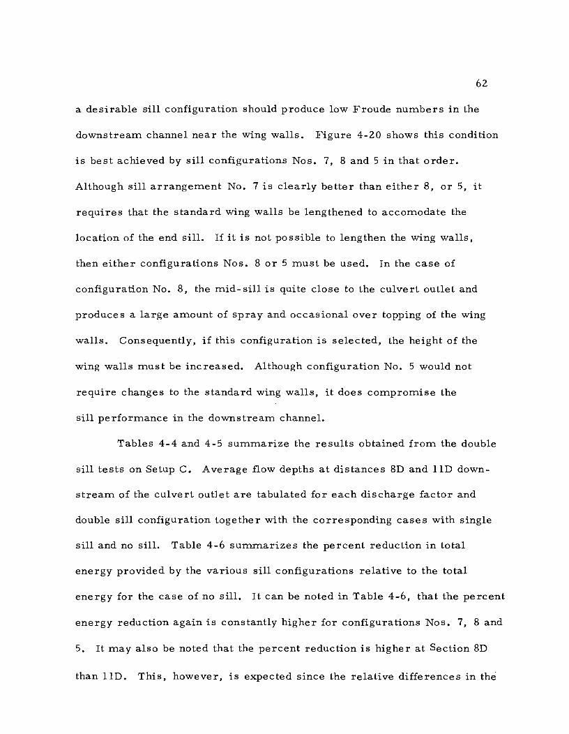
62

a desirable sill configuration should produce low Froude numbers in the

downstream channel near the wing walls. Figure 4-20 shows this condition

is best achieved by sill configurations Nos. 7, 8 and 5 in that order.

Although sill arrangement No. 7 is clearly better than either 8, or 5, it

requires that the standard wing walls be lengthened to accomodate the

location of the end sill. If it is not possible to lengthen the wing walls,

then either configurations Nos. 8 or 5 must be used. In the case of

configuration No.8, the mid- sill is quite close to the culvert outlet and

produces a large amount of spray and occasional over topping of the wing

walls. Consequently, if this configuration is selected, the height of the

wing walls must be increased. Although configuration No. 5 would not

require changes to the standard wing walls, it does compromise the

sill performance in the downstream channel.

Tables 4-4 and 4-5 summarize the results obtained from the double

sill tests on Setup C. Average flow depths at distances 8D and lID down­

stream of the culvert outlet are tabulated for each discharge factor and

double sill configuration together with the corresponding cases with single

sill and no sill. Table 4-6 surrunarizes the percent reduction in total

energy provided by the various sill configurations relative to the total

energy for the case of no sill. It can be noted in Table 4-6, that the percent

energy reduction again is constantly higher for configurations Nos. 7, 8 and

5. It may also be noted that the percent reduction is higher at Section 8D

than llD. This, however, is expected since the relative differences in the

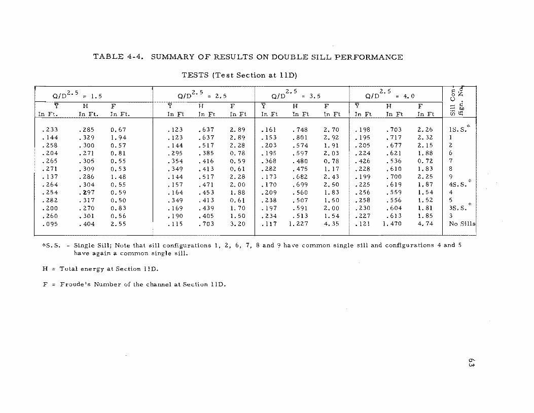
TABLE 4-4. SUMMARY OF RESULTS ON DOUBLE SILL PERFORMANCE

TESTS (Test Section at lID)

Q/D 2• 5 Q/D2• 5 Q/D

2.5 Q/D

2.5 g~ = 1.5 2.5 = 3.5 = 4.0 U .

Y H F Y H F Y H F Y H F ...... ~ ...... tlO

In Ft. In Ft. In Ft. In Ft In Ft In Ft In Ft In Ft In Ft In Ft In Ft In Ft U)~

.233 .285 0.67 · 123 .637 2.89 • 161 .748 2.70 .198 .703 2.26 15.5.*

. 144 .329 1. 94 .123 .637 2.89 · 153 .801 2.92 .195 .717 2.32 1

.258 .300 0.57 .144 .517 2.28 .203 .574 1. 91 .205 .677 2.15 2

.204 .271 0.81 .295 .385 0.78 • 195 .597 2.03 .224 .621 1. 88 6

.265 .305 0.55 .354 .416 0.59 .368 .480 0.78 .426 .536 0.7Z 7

.271 .309 0.53 .349 .413 0.61 .282 .475 1. 17 .228 .610 1. 83 8

. 137 .286 1. 48 .144 .517 2.28 · 173 .682 2.43 .199 .700 2.25 9

.264 .699 .619 1. 87 ~:t

.304 0.55 • 157 .471 2.00 • 170 2.50 .225 45.5 • .254 . Z97 0.59 .164 .453 1. 88 .209 .560 1. 83 .256 .559 1. 54 4 .282 . 317 0.50 .349 .413 0.61 .238 .507 1. 50 .258 .556 1. 52 5 .200 .270 0.83 · 169 .439 1. 70 · 197 .591 2.00 .230 .604 1. 81 35. S. ':'

.260 .301 0.56 · 190 .405 1. 50 .234 .513 1. 54 .227 .613 1. 85 3

.095 .404 2.55 .115 .703 3.20 .117 1. 227 4.35 • 121 1. 470 4.74 No Sills

':<5. S. - Single Sill; Note that sill configurations I, 2, 6, 7, 8 and 9 have COITlITlon single sill and configurations 4 and 5 have again a COITlITlOn single sill.

H = Total energy at Section lID.

F = Froude's NUITlber of the channel at Section llD.

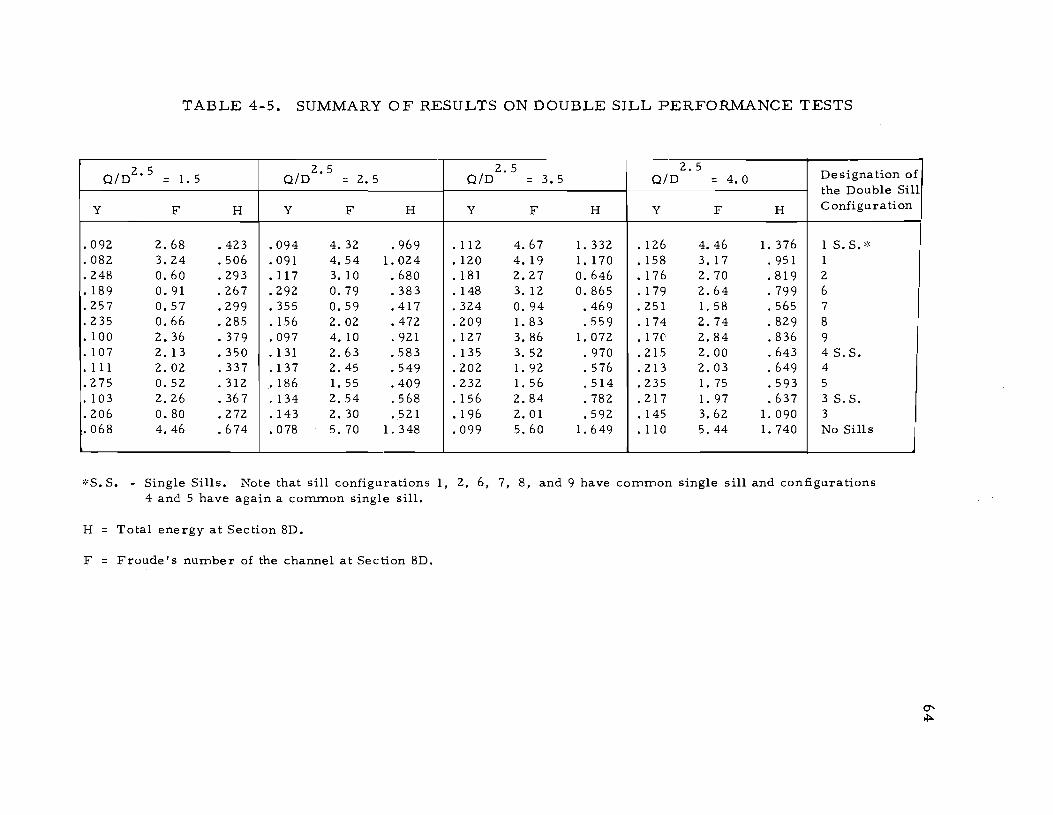
TABLE 4-5. SUMMARY OF RESULTS ON DOUBLE SILL PERFORMANCE TESTS

a/D2. 5 2.5 2.5 2.5 Designation of = 1.5 aiD = 2.5 aiD = 3.5 aiD = 4.0 the Double Sill

y F H Y F H Y F H Y F H Configuration

.092 2.68 .423 .094 4.32 .969 · 112 4.67 1. 332 · 126 4.46 1. 376 1 S. S. ':'

.082 3.24 .506 .091 4.54 1. 024 • 120 4. 19 1. 170 · 158 3. 17 . 951 1

.248 0.60 .293 • 117 3. 10 .680 · 181 2.27 0.646 • 176 2.70 .819 2

.189 O. 91 .267 .292 0.79 .383 · 148 3. 12 0.865 · 179 2.64 .799 6

.257 0.57 .299 .355 0.59 .417 .324 0.94 .469 .251 1. 58 .565 7

.235 0.66 .285 · 156 2.02 .472 .209 1. 83 .559 .174 2.74 .829 8

.100 2.36 .379 .097 4. 10 .921 .127 3.86 1. 072 · 17(' 2.84 .836 9

.107 2. 13 .350 · 131 2.63 .583 · 135 3.52 .970 .215 2.00 .643 4 S. S • • 1 11 2.02 .337 · 137 2.45 .549 .202 1. 92 .576 .213 2.03 . 649 4 .275 0.52 .312 · 186 1. 55 .409 .232 1. 56 .514 .235 1. 75 .593 5 . 103 2.26 .367 .134 2.54 .568 .156 2.84 .782 . 217 1. 97 .637 3 S. S . .206 0.80 .272 .143 2. 30 .521 .196 2.01 .592 .145 3.62 1. 090 3 .068 4.46 .674 .078 5.70 1. 348 .099 5.60 1.649 • 110 5.44 1. 740 No Sills

':'S.S. - Single Sills. Note that sill configurations 1, 2, 6, 7, 8, and 9 have conUTIon single sill and configurations 4 and 5 have again a conunon single sill.

H Total energy at Section 8D.

F = Froude's nUI1lber of the channel at Section 8D.

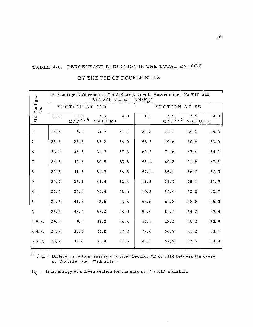
65

TABLE 4-6. PERCENTAGE REDUCTION IN THE TOTAL ENERGY

BY THE USE OF DOUBLE SILLS

Percentage Difference in Total Energy Levels Between the 'No Sill' and I=i 'With Sill' Cases ( c\H/Ho)':' bIl .... ...... I=i SECTION 0 0

AT lID SECTION AT 8D

uz .-< 1.5 2.5 3. 5 4.0 1.5 2.5 3. 5 4.0 .-<

Q/D 2 • 5 Q/D 2 • 5 .... VALUES VALUES U)

1 18.6 9.4 34.7 51. 2 24.8 24. 1 29.2 45.3

2 25.8 26.5 53.2 54.0 56.2 49.6 60.6 52.9

6 33.0 45.3 51. 3 57.8 60.2 71. 6 47.6 54.1

7 24.6 40.8 60.8 63.6 55.4 69.2 71. 6 67.5

8 23.6 41. 3 61. 3 58.6 57.4 65. 1 66.7. 52.3

9 29.3 26.5 44.4 52.4 43.5 31. 7 35. 1 51. 9

4 26.5 35.6 54.4 62.0 49.2 59.4 65.0 62.7

5 21. 6 41. 3 58.6 62.2 53.6 69.8 68.8 66.0

3 25.6 42.4 58.2 58.3 59.6 61. 4 64.2 37.4

1 S. S. 29.5 9.4 39.0 52.2 37.3 28.2 19.3 20.9

4 S. S. 24.8 33.0 43.0 57.8 48.0 56.7 41. 2 63. 1

3 S. S. 33.2 37.6 51. 8 58.3 45.5 57.9 52.7 63.4

>!' , .:.\ H = Difference is total energy at a given Section (8D or lID) between the cases

of 'No Sills' and 'With Sills' •

Ho Total energy at a given section for the case of 'No Sill' situation.

66

perforITlance of the various double sill patterns are ITlore pronounced near

the culvert outlet. On the other hand, it is recognized that ITleasureITlents

ITlade near the culvert outlet, i. e., at 8D, are ITlore 8usceptible to error

than corresponding ITleasureITlents ITlade further downstreaITl.

Double Sill Tests on Concrete Pipe Models

All results on the perforITlance of double sills presented above were

obtained with a corrugated ITletal pipe culvert (Setup C). Based on these

results it was found that extensive testing with the concrete pipe ITlodels

was not required. A few trial runs indicated, however, that the selected

double sill configurations for corrugated ITletal pipe ITlodels were not

necessarily suitable for the concrete pipe ITlodels.

Rather it was found that the relative spacing of sills ( ~\X) needed

to be increased in order to dissipate the energy of higher velocity flows

obtained with two concrete pipe ITlodels. Accordingly the best double sill

configuration for the concrete pipe corresponds to the following diITlensions:

Xl = 1. 5D, Xl = 4.6D, sl = O. 167D with the ITlid-sill height varying

between O. 5D and O. 556D depending upon the setup. The data froITl the

concrete pipe Setups D to G are sUITlITlarized in Appendix A, Tables A-Il

through A-l6.

To illustrate the perforITlance of double sills with the concrete pipe,

transverse depth and velocity profiles were again ITleasured for representative

67

discharge factors and different culvert geometries. These data shown in

Figures 4-21 through 4-31 indicate that sills produce a consistent and

marked increase in depths (corresponding to reduction in velocities) at

Sections 8D and lID downstream of the culvert outlet. The relative

pe rformances of double sills together with the 'no sill' case are

summarized in Table 4-7 which also includes corresponding energy levels

in the downstream channel. Table 4-7 shows an average energy reduction

of 73% at Section lID if sills are used. This percentage reduction is

indicative of the effectiveness of the sills. Furthermore, the percent

energy change between the upstream section of the hydraulic jump and the

11 D section was found to be about 86% on average although this energy

change varied with the culvert configuration and the discharge factor.

.26

.22

t-= .18 SETUP 0 ll.. Q 10 2.5 = 3.50 XI = 1.5 0 X2 = 4.6 0 z 0 NO SILLS } 80 SECTION 51 = 0.556 0 52 = 0.1670

I <D WITH SILLS 5: .14

& NO SILLS } II 0 SECTION w

0 &. WITH SILLS CD

.10

.06

5 7 9 CHANNEL WIDTH IN FT.

Figure 4-21. Downstream. Channel Transverse Depth Profiles

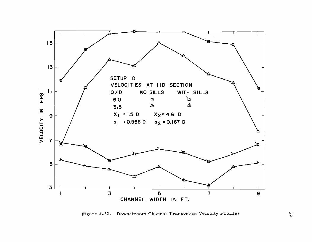
15

13

SETUP 0 VELOCITIES AT 110 SECTION

II Q/O NO SILLS WITH SILLS en a.. 6.0 r:J G u..

z 3.5 8 Lh

9 XI = 1.5 0 X2 = 4.6 0 ~ = 0.556 0 52. = 0.167 0 ~ 51 0

9 LaJ

7 >

5

3 ~ ______ ~ ______ ~ ____ ~ ______ ~ ____ ~ ______ -L ______ L-____ ~~

3 5 7 9 CHANNEL WIDTH IN FT.

Figure 4-22. Downstream Channel Transverse Velocity Profiles

.24 SETUP E

0 NO SILLS } SECTION) <D WITH SILLS (80

.20 QI 0 2.5 = 1.50

XI = 1.5 0 X2 =4.S 0 ~ SI = 0.5 0 S2 =0.IS7 0 LL

z .IS

::I: J-a. w 0 .12

.08

.04~ ______ ~ ______ ~ ____ ~ ______ ~ ______ ~ ______ ~ ____ ~ ______ ~~

3 5 7 9 CHANNEL WIDTH IN FT.

Figure 4-23. Downstream Channel Transverse Depth Profiles

.50

. f- .40 LL

SETUP E Q / 0 2.5 = 6.00

o NO SILLS }- (80 SECTION) (]) WITH SI LLS

X I = 1.5 0

S I = 0.5 0

X2 = 4.6 0

S 2 = 0.1670

Z ~------ID-

~ .30 ~ ~------¢h--____ ~------~

w a

.20

. 10

•

3 5 7 9 CHANNEL WIDTH IN FT.

Figure 4-24. Downstream Channel Transverse Depth Profiles

15

13

en 1 1 a.. LL

Z

>- 9 I-o 9 lLJ > 7

5

S I :: 0.5 0

X2 :: 4.60

NO SILLS

SETUP E ALL VALUES AT 80 SECTION

3~c=====~====~====~~ ____ l-____ -L ____ ~ ______ ~ ____ ~

3 5 7 9

CHANNEL WIDTH IN FT.

Figure 4-25. Downstream. Channel Transverse Velocity Profiles -J N

.25~,-----~------~----__ ~----~------~~----~----~------~

.20

i-= .15 li..

z

J:

h: .10 w o

.05

SETUP F Q /D2.5 = 2.50

o NO SILLS } 8D CD WITH SILLS

SECTION

SECTION Il:J. NO SI LLS } & WITH SILL II D .00 ~ ______ ~ ______ ~ ____ ~ ______ -L ______ ~ ______ L-____ -L ______ ~

:3 5 7 9

CHANNEL WIDTH IN FT.

Figure 4-26. Downstream Channel Transverse Depth Profiles

.301l-------.------~~--~~----~------~------~----~------___

.25

SETUP F ...=

.20 Q/D2 .5= 3.50 ll...

z (8D SETION) { 0 NO SILLS <D WITH SILLS /

::I: ~ I-

SECTION) { NO SILLS

Cl. .15 ( II D Lt w WITH SILLS 0

.10 XI = 1.5D X2=4.6 D

sl =0.556D s2=0.167D

.05~~~ __ ~ ______ ~ ____ ~L-____ -L ______ ~ ______ L-____ ~ ______ ~

3 5 7 9

CHANNEL WIDTH IN FT.

Figure 4-27. Downstream. Channel Transverse Depth Profiles

(J) Q.. LL

22

18

z 14

>-I-o 9 10 IJJ >

6

SETUP F Q /02.5

1.5

2,5 3,5 6.0

NO SILLS WITH SILLS XI = 1,5 D X2 = 4.6 D <D 0 5r = 0.5560 52 = 0,167 D 0 0 & ~ b G

2 ~~ ______ ~ ______ ~ ______ ~ ______ ~ ______ ~ ______ ~ ______ ~ ______ ~~ 5 7 9

CHANNEL WIDTH IN FT.

Figure 4-28. Downstream Channel Transverse Velocity Profiles

.25~~----~------~------~------~----~------~------~------~

SETUP G Q 102.5 : 2.50

.20

r-: LL

.15 z 0 NO SILLS }

WITH SI LLS (80 SECTION) (J) :::t:

6. NO SILLS } l-e.

~ WITH SILLS w .10 CI

.05 XI = 1.5 0 X2: 4.6 0

S I = 0.5560 s2: 0.1670

0.0 3 5 7 9

CHANNEL WIDTH IN FT.

Figure 4-29. Downstream Channel Transverse Depth Profiles

.30 II------~------~------~------~----~------~------~------~

t-= lL.

.25

z .20

::I: l­e. ~ .15

.10

SETUP G

Q/O =3.50

o NO SILLS } 80 <D WITH SILLS SECTION

& NO SILLS } Lh WITH SILLS 110 SECTION

X 1= 1.5 0 X2 = 4.6 0 S I = 0.5560 s2 = 0.167 0

.05 ~~-------~----~------~-------~-------~------~------~------~~ 5 7 9

CHANNEL WIDTH IN F~

Figure 4-30. Downstream Channel Transverse Depth Profiles

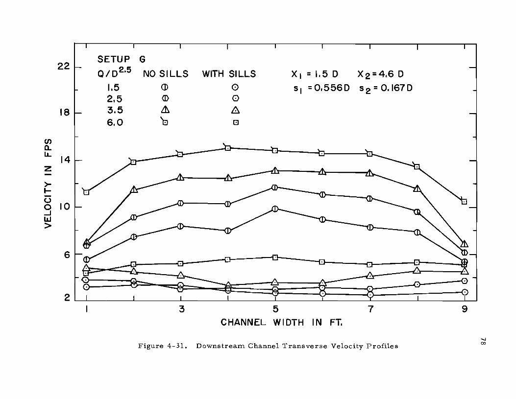
CJ) Q.

22

18

11. 14 z ~ I-

g 10 -I l1J >

6

SETUP

Q/D 2 .5

1.5 2.5 3.5 6.0

G

NO SILLS WITH SILLS XI = 1.5 D X2 =4.6 D CD 0 S I = 0.556D s2 = 0.167D <D 0 ~ ~ b [!)

2 L-L-______ ~ ______ ~ ______ _L ______ ~ ________ ~ ______ ~ ______ ~ ______ ~~

3 5 7 9 CHANNEL WIDTH IN FT.

Figure 4-31. Downstream Channel Transverse Velocity Profiles ....... OJ

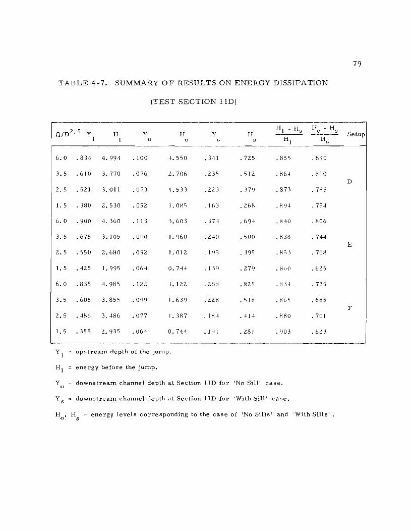
TABLE 4-7. SUMMARY OF RESULTS ON ENERGY DISSIPATION

Q/D 2 . 5 y 1

H 1

6.0.8344.994

3.5 .610 3.770

2.5.5213.011

1.5.3802.530

6.0.9004.360

3.5.6753.105

2.5.5502.680

1. 5 • 425 1. 995

6.0.8354.985

3.5.6053,85<;

2.5 .486 3. 486

y

.100

.076

.073

.052

. 113

.090

.092

.064

• 122

.099

.077

(TEST SECTION lID)

H y o o

4.550 .341

2.706 .23'1

1.533 .223

1.08'1 .1(,3

3. 603 .374

I. 960 .240

I. 012 • I 1l5

0.744 · I 3!)

3. 122 .288

1.639 .228

1.387 .184

II - H H

o s

.725 .855 .840

.512 .86..J .810

.379 .873 .755

.268 .894 .754

.694 .840 .806

.500 .838 .744

.395 .8'13 .708

.279 .8ll0 .625

.82'1 .834 .735

. '118 .80<; .685

.414 .8HO .701

79

Setup

D

E

F

.064 0.744 • 141 .281 1.5.355 2.935 . 1)03 .623 J '--

y 1 upstream depth of the jump.

HI energy before the jump.

Y downstrearn channel depth at Section lID for 'No Sill' case. o

Y s downstrearn channel depth at Section lID for 'With Sill' case.

H ,H = energy levels corresponding to the case of 'No Sills' and With Sills' . o s

CHAPTER V

SUMMARY AND CONCLUSIONS

Based on tests conducted on the hydraulic performance of 18-inch

corrugated metal pipe and concrete pipe culvert models the following

conclusions are jus tified:

1. The head water depth-discharge factor relationships for corrugated metal and concrete pipe culverts operating with sharp edged entrances are identical up to a discharge factor, Q!D2 . 5 = 2.5.

2. Under ventilated conditions the corrugated metal pipe displayed a slug and mixture control in the range of 2. 5 .~~ Q!D2 • 5 -c::. 4.5 whereas the concrete pipe displayed an orifice control in the range of Z.5.c::::Q!D Z. 5 <.::: 6.5. BeyondQ!D2 . 5 = 4.5 the corrugated metal pipe operated under pipe control.

3. The hydraulic jump in the steep sloped corrugated metal pipe cuI vert models were influenced significantly by the presence of horizontal unit (Unit 3) and the sharp change in grade between Unit 2 and Unit 3 where­as the jump position was little affected in the case of concrete pipe culvert models operated with similar geometrical configurations and discharge factors.

4. A jump can be produced without a sill for cases in which Unit 3 was sufficiently long or rough to cause critical depth to be obtained in the horizontal section of the culvert.

5. A sill was necessary to force a hydraulic jump to form inside the culvert for those cases where there was either an absence or insufficient length of horizontal unit at the end of steep unit of the culvert. For the culvert configurations and discharge factors

80

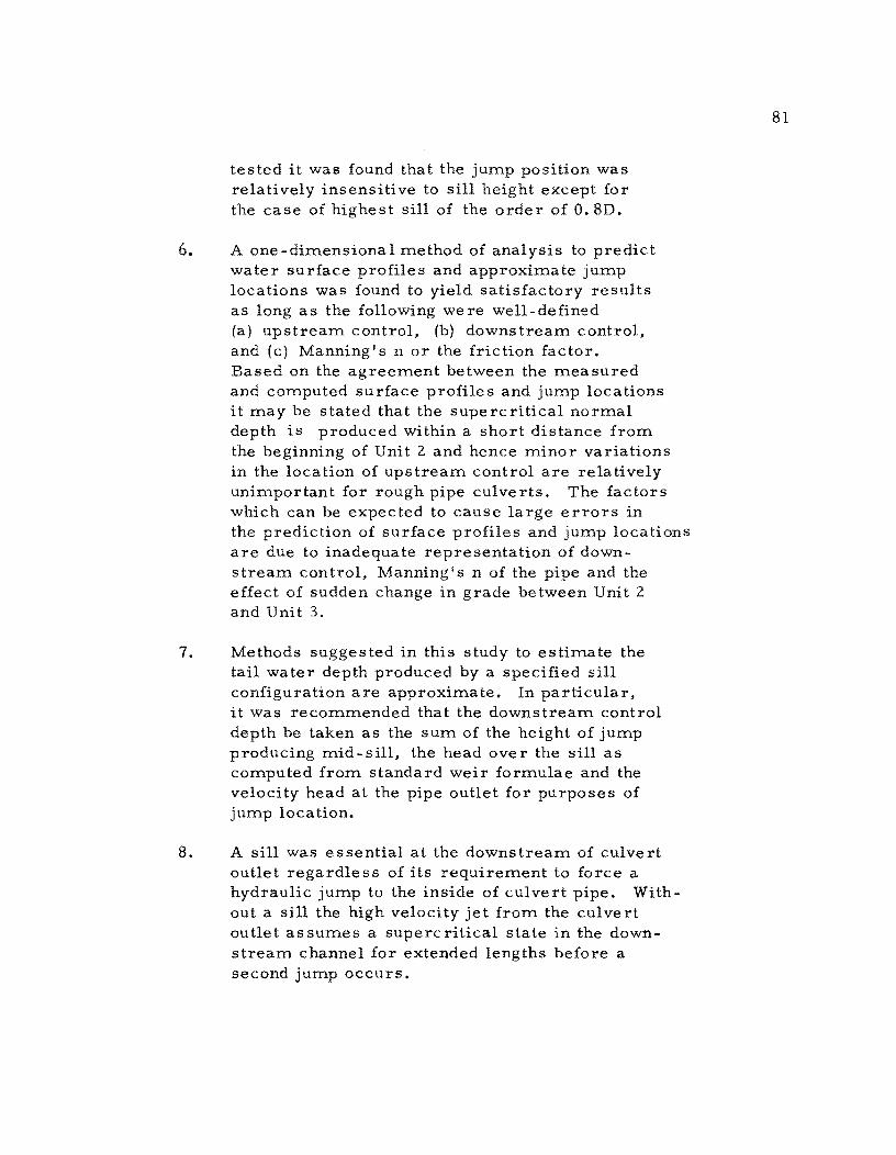
tested it was found that the jump position was relatively insensitive to sill height except for the case of highest sill of the order of O. 8D.

6. A one-dimensional method of analysis to predict water surface profiles and approximate jump locations was found to yield satisfactory results as long as the following were well-defined (a) upstream control, (b) downstream control, and (c) Manning's 11 or the friction factor. Based on the agreement between the measured and computed surface profiles and jump locations it may be stated that the supercritical normal depth is produced within a short distance from the beginning of Unit 2. and hence minor variations in the location of upstream control are relatively unim.portant for rough pipe culverts. The factors which can be expected to cause large errors in the prediction of surface profiles and jump locations are due to inadequate representation of down­stream control, r-1anning ' s n of the pipe and the effect of sudden change in grade between Unit 2 and Unit 3.

7. Methods suggested in this study to estimate the tail water depth produced by a specified sill configuration are approximate. In particular, it was recommended that the downstream control depth be taken as the sum of the height of jump producing mid-sill, the head over the sill as computed from standard weir formulae and the velocity head at the pipe outlet for purposes of jump location.

8. A sill was essential at the downstream of culvert outlet regardless of its requirement to force a hydraulic jump to the inside of culvert pipe. With­out a sill the high velocity jet from the culvert outlet assumes a supercritical state in the down­stream channel for extended lengths before a second jump occurs.

81

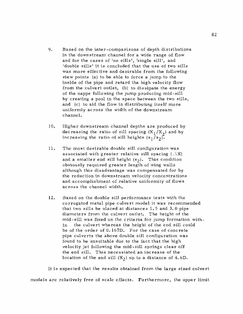
9. Based on the inter-comparisons of depth distributions in the downstream channel for a wide range of flow and for the cases of 'no sills', 'single sill', and 'double sills' it is concluded that the use of two sills was more effec ti ve and de sirable from the following view points (a) to be able to force a jump to the inside of the pipe and retard the high velocity flow from the culvert outlet, (b) to dissipate the energy of the nappe following the jump producing mid- sill by creating a pool in the space between the two sills, and (c) to aid the flow in dis tributing itself more uniformly ac ross the width of the downstream channel.

10. Higher downstream channel depths are produced by dec reasing the ratio of sill spacing (X 1 /X

2) and by

increasing the ratio of sill heights (sl/s2)'

11. The most desirable double sill configuration was associated with greater relative sill spacing ( .\X)

and a smaller end sill height (s2)' This condition obviously required greater length of wing walls although this disadvantage was compensated for by the reduction in downstream velocity concentrations and accomplishment of relati ve uniformi ty of flows across the channel width.

12. Based on the double sill performance tests with the corrugated metal pipe culvert model it was recommended that two sills be placed at distance s 1. 5 and 3. a pipe diameters from the culvert outlet. The height of the mid-sill was fixed on the criteria for jump formation with­in the culvert whereas the height of the end sill could be of the order of O. 167D. For the case of concrete pipe cuI verts the above double sill configuration was found to be unsuitable due to the fact that the high velocity jet following the mid-sill springs clear off the end sill. This necessiated an increase of the location of the end sill (X2 ) up to a distance of 4. 6D.

It is expected that the results obtained from the large sized culvert

models are relatively free of scale effects. Furthermore, the upper limit

82

of the experimental range corresponds to the extremes in regard to both

the discharge factor as well as the steepness of Unit 2. Hence the

experimentally observed values in this study are believed to adequately

represent the hydraulic state of affairs associated with prototype culvert

ins tallations.

83

REFERENCES

1. Price, B. E., and Masch, F. D., 1967. "Performance of Circular Culverts on Steep Grades", Research Report Number 92-2, Center for Highway Research, The University of Texas at Austin.

2. Brandes, R. J., Masch, F. D., and Rao, Manam V. P., 1969. "End Sills and the Forced Hydraulic Jump in Circular Culverts Operating at Low Discharge Factors", Research Report Number 92-4, Center for Highway Research, The University of Texas at Austin.

3. MacDonald, T. C., 1969. "Energy Dissipators for Large Culverts", Journal of the Hydraulic Division, ASCE, Vol. 95, No. HY 6, November 1969, pp. 1941-1958.

4. Blaisdell, F. W., 1966. "Culve rt Flow and Related De sign Philosophies", Journal of the Hydraulic Division, ASCE, Vol. 92, No. HY 2, March 1966, pp. 19-31.

5. French, J. L., 1961. "Fourth Progress Report on Hydraulics of Culverts - Hydraulics of Improved Inlet Structures for Pipe Culverts", National Bureau of Standards Report No. 7178, 132 pp.

84

APPENDIX

(Data Tables)

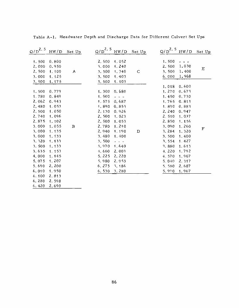
Table A-I. Headwater Depth and Discharge Data for Different Culvert Set Ups

Q/D2

.5

HW/D Set Up Q/D2

.5

HW/D Set Up

1. 500 O. 800 2. 500 L 052 1. 500 2. 000 0.950 3. 000 1. 240 2.500 1. 030

E 2.500 1. 100 A 3.500 1.340 C 3.500 1. 400 3. 000 1. 125 3.500 L 403 6. 000 1.968 3.500 1. 17 5 3.500 1. 103

1. 018 0.600 1. 500 0.779 1. 300 O. 680 1. 270 O. 673 1. 780 0.849 1.500 1. 450 0.730 2. 062 0.943 1. 575 0.687 1. 765 O. 81 '3 2. 480 1. 053 1. 890 0.853 1. 890 O. 883 2.500 1. 050 2. 130 0.926 2. 240 0.947 2. 740 1. 096 2.500 1. 023 2. 510 1.037 2.875 1. 102 2.500 1. 053 2. 850 1. 1 56 3. 000 1. 055 B 2. 780 1. 210 3.090 1. 260

F 3. 000 1. 135 2. 940 1. 190 D 3. 284 1.320 3.000 1. 133 3. 480 1. 400 3.500 1. 400 3.320 1. 133 3. 500 ::\. 554 1.427 3.500 1. 133 3.970 1. 640 3. 880 1. 613 3.635 1. 153 4. 660 2.003 4. 220 1.792 4. 000 1. 145 5.225 2.220 4.570 1. 967 5.075 1. 207 5.980 2.9')3 5. 040 2. 317 5.690 2.200 6.275 3. 186 '5. 580 2. 687 6. 010 1.950 6. 530 3. 280 5.9QO 1. 967 6.100 2.813 6. 280 2.598 6. 420 2. 0

86

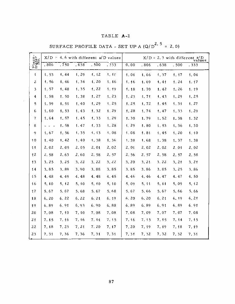
TABLE A-2

SURFACE PROFILE DATA - SET UP A (Q/D2

. 5 = 2.0)

I ~~. X/D = 4. 6 with different s/ D values X/D = 2. :3 with different s{D N....,O va ues <l)(UZ;

.806 .750 .638 .500 . 333 0.00 .806 .638 .500 .333 I 0":6

1 1. 53 1. 44 1.29 1. 12 1. H' 1. 01 1. 66 1. 37 1.17 1. 04

2 1. 56 1. 46 1. 34 1. 20 1. 16 1. 16 1. 69 1. 41 1. 24 1.17

3 1. 57 1. 48 1. 35 1. 22 1. 19 1. 18 1. 70 1. 42 1. 26 1. 19

4 1. 58 1. 50 1. 38 1. 27 1. 23 1. 23 1. 71 1. 43 1. 29 1. 25

5 1. 59 1. 51 1. 40 1.29 1. 25 1. 25 1.72 1. 45 1. 31 1. 27

6 1. 60 1. 53 1. 43 1. 32 1. 29 1. 28 1. 74 1. 47 1. 33 1. 29

7 1. 64 1. 57 1. 45 1. 33 1. 29 1. 30 1. 79 1. 52 1. 38 1. 32

8 - - - 1. 58 1. 47 1. 33 1. 28 1. 29 1. 80 1. 53 1. 36 1. 30

9 1. 67 1. 56 1. 35 1.13 1. 08 1. 08 1. 81 1. 45 1. 20 1. 10

10 1. 40 1. 42 1. 40 1. 38 1. 36 1. 38 1. 68 1. 38 1. 37 1. 38

11 2. 02 2. 05 2.05 2. 01 2. 02 2. 01 2. 02 2. 02 2. 01 2. 02

12 Z.58 2. 63 2.60 2. 58 2. 57 2.56 2. 57 2. 58 2. 57 2. 58

13 3.25 3. 25 3. Z2 3.22 3. Z2 3. 20 3. 21 3. 22 3. 21 3. 21

14 3.85 3. 89 3.90 3. 88 3.85 3. 85 3. 86 3.85 3. 25 3. 86

15 4. 48 4. 49 4.48 4. 48 4.45 4.46 4. 46 4.47 4.47 4. 50

16 5. 10 5. 12 5. 10 5. 10 5. 10 5. 09 5.11 5.11 5. 09 5. 12

17 5. 67 5.67 5. 68 5. 67 5.68 5. 67 5. 66 5. 67 5.66 5. 66

18 6. 20 6. 22 6.22 6. 21 6. 19 6. 20 6. 20 6.21 6. 19 6. 21

19 6. 89 6.91 6.93 6.90 6. 88 6.89 6. 89 6.91 6. 89 6.91

20 7.08 7. 10 7. 10 7.08 7.08 7.08 7.09 7.07 7.07 7.08

21 7. 15 7. 16 7. 16 7. 14 7. 15 7. 16 7. 15 7. 15 7. 14 7. 15

22 7. 18 7.23 7. 21 7.20 7.17 7.20 7. 19 7. 19 7. 18 7.19

23 7. 31 7.36 7.36 7. 31 7.31 7. 31 7.32 7.32 7. 32 7. 31

87

TABLE A-3

2 5 SURFACE PROFILE DATA - SET UP A (Q/D . 2.5)

X/D :;; 4.6 with different sID Values xl D:;; 2. 3 with different sl D ~

0 Z; .806 .750 .694 .638 . 557 . 503 .333 0.00 .806 ,638 . 500 .333

i 1 1. 54 L 48 1.42 1. 34 1. 24 1. 19 1. 10 1.11 1.71 1. 45 L 23 1. 13

2 1. 57 L 53 1. 48 1. 40 1.34 1. 32 1. 28 1. 28 1. 75 1. 50 1. 32 1. 27

3 1. 58 1. 54 1. 49 1. 42 1. 36 1. 35 1. 31 1. 32 1. 76 1. 52 L 34 1. 31

4 1. 61 1. 57 L 53 1. 46 L 41 L 39 1. 36 1. 36 1. 78 1. 54 1. 39 L 36

5 1. 63 1. 58 1. 54 1. 49 L 43 1.42 1. 39 1. 40 1. 79 1. 55 L 42 1. 38

6 1. 65 1. 61 1. 57 L 52 1. 47 1. 45 1.42 1. 42 1. H2 L 57 1. 44 1. 41

7 1. 73 1. 68 1. 62 1. 58 1. 54 1. 52 1. 48 1. 49 1. 8Ci 1.64 L 52 L 49

8 1. 75 1. 71 1. 65 1. 61 1. 55 1. 53 1. 49 1. 49 1. 91 1. 65 1. 52 L 49

9 1. 76 1. 70 1. 62 1. 54 1. 44 1. 42 1. 32 1. 30 l.'j"l; 1. 63 1. 38 L 32

10 1. 48 1. 48 1. 47 1. 47 1. 46 1. 44 1. 45 1. 44 1 87 1. 45 1. 45 L 45

11 2.09 2.09 2. 09 2. 09 2.07 2.06 2. OH 2.07 2.10 2. 08 2. 08 2. 08

12 2.65 2.65 2.64 2.63 2.63 2. 63 2. 62 2. 62 2, h6 2. 64 2. 62 2.62

13 3.30 3.31 3. 29 3.26 3.27 3.27 3. 26 3. 27 3. W 3.28 3.28 3. 28

14 3.93 3.93 3.94 3.9':\ 3.92 3.9':\ 3. 91 3.93 3. <)"' 3.95 3.92 3.93

15 4. 55 4. 55 4. 54 4. 5'1 4. 52 4. 54 4. 53 4.52 4.54 4. 53 4.54 4. 53

16 5. 17 5.18 5. 15 5.16 5.17 5.16 5. 16 5. 17 5. 19 5. 19 5.17 5. 17

17 5. 70 5.72 5. 71 5.70 5.72 5. 71 5. 70 5. 70 5. 75 5. 70 5.70 5. 70

18 6.26 6. 27 6. 26 6.25 6. 27 6.24 6. 24 6.25 6.28 6. 27 6.25 6. 27

19 6.98 6.99 7.00 7.00 7.01 6.98 6.98 6.99 6.98 6.98 6.98 6.97

20 7. 15 7.15 7.15 7.15 7.13 7.14 7.13 7. i 5 7. 15 7. i 5 7. 15 7.1.4

21 7.20 7.20 7.20 7.21 7. 19 7.20 7. 19 7.2f 7,23 7.23 7.23 7,23

22 7.25 7.26 7.24 7.2.5 7.23 7.24 7.23 7.24 7.26 7.28 7.27 7.27

23 7.40 7.38 7.37 7.36 7.39 7.39 7.40 7.41 7.45 7.44 7,44 7.44 I

88

TABLE A-4

/ 2. 5

SURFACE PROFILE DATA - SET UP A (Q D = 3. 0)

I X/D = 4.6 with different siD Values X/D = 2.3 with different siD values 0 ..... NQ)O

.806 .750 .694 .638 . 500 .333 0.00 .806 .638 .500 .333 Q)Q1Z;

P:s 1 1. 59 1. 53 1. 46 1. 39 1. 25 1.17 1.17 1.77 1. 46 1. 31 1. 22

2 1. 65 1. 59 1. 53 1. 48 1. 39 1. 36 1. 36 1. 82 1. 54 1. 43 1. 40

3 1. 67 1. 61 1. 56 1. 51 1. 44 1. 40 1.40 1. 84 1. 56 1. 47 1. 44

4 1. 69 1. 65 1. 60 1. 56 1. 48 1.45 1. 46 1. 87 1. 59 1. 52 1. 51

5 1.72 1. 67 1.62 1. 58 1. 51 1. 48 1. 48 1. 89 1. 61 1. 55 1. 52

6 1. 75 1. 69 1. 64 1. 61 1. 55 1. 52 1. 52 1. 92 1. 65 1. 58 1. 56

7 1. 87 1. 80 1. 75 1.72 1. 65 1. 63 1. 62 2.03 1. 75 1. 67 1. 65

8 1. 88 1. 84 1. 79 1. 74 1. 67 1. 65 1. 65 2. 04 1. 76 1. 69 1. 67

9 1. 91 1. 88 1. 8') 1. 79 1. 68 1. 65 1. 65 2.07 1. 77 1. 67 1. 63

10 2.03 1. 96 1. 89 1. 83 1. 45 1. 43 1. 42 2.17 1. 54 1. 55 1. 55

11 1. 95 1. 95 1. 9 ') 1. 94 2.07 2. 02 2.02 2. 14 2. 16 2. 15 2. 15

12 2.58 2. 57 2. 58 2.56 2.59 2. 59 2.60 2. 70 2. 71 2. 70 2. 69

13 3.23 . 3.23 3.2') 3. 23 3. 24 3.20 3.25 3.35 3. 35 3.35 3. 35

14 3.86 3. 87 3.83 3. 84 3.90 3. 87 3.88 4.01 4.02 4.01 4.01

15 4.48 4. 47 4.46 4.45 4.49 4.49 4.49 4.63 4. 62 4.61 4. 61

16 5. 19 5. 18 5. 21 5. 00 5.13 5.11 5. 16 5.25 5.25 5.25 5.25

17 5. 70 5.72 5. 73 5.71 5. 74 5.69 5. 69 5.80 5.77 5.77 5. 80

18 6. 27 6. 34 6.30 6. 27 6.23 6.21 6. 22 6. 34 6. 35 6. 34 6. 32

19 7.01 7.05 7.01 7.02 6.98 6.95 6.93 7.08 7.08 7.08 7.10

20 7.12 7. 12 7.15 7. 09 7.10 7. 10 7. 10 7.26 7.25 7.25 7.26

21 7.19 7. 19 7.17 7. 18 7.17 7. 16 7.18 7.34 7.33 7.33 7.33

22 7.26 7.25 7.26 7.24 7.22 7.22 7.22 7.43 7.43 7.43 7.44

23 7.43 7.42 7.41 7. 37 7.38 7.38 7.38 7.54 7.54 7.54 7.54

89

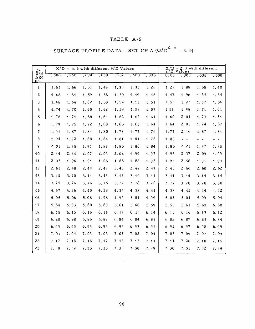
TABLE A-5

/ 2. 5

SURFACE PROFILE DATA - SET UP A (Q D = 3. 5)

'"" x/D = 4.6 with different sl D Values XjD = 2.3 with different

OQ) • s D Values N ..... O • ~Ob .750 • b9t • b3~ . 557 . 5UU . 333 O. 00 . ~Ob . b38 .500 ~!f

1 1. 61 1. 56 1. 51 1. 43 1. 36 1. 32 1. 26 1. 28 1. 88 1. 58 1. 40

2 1. 68 1. 61 1. 59 1. 56 1. 50 1. 49 1. 48 1. 47 1. 96 1. 65 1. 54

3 1. 68 1. 64 1. 62 1. 58 1. 54 1. 53 1. 51 1. 52 1. 97 1. 67 1. 56

4 1. 74 1. 70 1. 65 1.62 1. 58 1. 58 1. 57 1. 57 1. 98 1. 71 1. 61

5 1. 76 1. 71 1. 68 1. 64 1. 62 1. 62 1. 61 1. 60 2. 01 1. 73 1. 64

6 1. 79 1. 75 1.72 1. 68 1. 65 1. 63 1.64 1. 64 2.05 1. 74 1. 67

7 1. 91 1. 87 1. 84 1. 80 1. 78 1.77 1. 76 1.77 2. 16 1. 87 1. 81

8 1. 94 1. 92 1. 88 1. 84 1. 81 1. 81 1. 78 1. 80 - - - - - -

9 2.01 1. 95 1. 91 1. 87 1. 85 1. 86 1. 84 1.85 2. 23 1. 97 1. 85

10 2.14 2.11 2.07 2. 03 2.02 1. 99 1. 97 1. 96 2. 37 2. 09 1. 99

11 2.05 1. 96 1. 91 1. 86 1. 85 1. 86 1. 92 1. 93 2. 56 1. 95 1. 93

12 2. 51 2. 48 2.49 2.49 2.49 2.48 2.47 2.45 2. 50 2. 50 2. 52

13 3. 15 3. 10 3.11 3.13 3.12 3. 10 3.11 3. 11 3.14 3.14 3.14

14 3. 74 3. 76 3. 76 3.75 3. 74 3. 76 3.76 3.77 3. 78 3. 78 3. 80

15 4. 37 4. 36 4.40 4.38 4.39 4. 38 4.41 4. 38 4. 42 4.44 4. 42

16 5.05 5. 06 5.08 4.98 4.98 5.01 4.99 5. 02 5. 04 5. 09 5.04

17 5.64 5.63 5.60 5. 60 5.61 5. 60 5. 59 5. 55 5.61 5. 63 5. 60

18 6.15 6.15 6. 16 6.14 6.13 6. 12 6.14 6.12 6. 16 6.13 6. 12

19 6. 88 6. 88 6. 86 6. 87 6. 84 6. 84 6.83 6.82 6. 87 6.85 6. 84

20 6.93 6.93 6.93 6.93 6.93 6.93 6.95 6.92 6. 97 6.98 6.99

21 7.03 7.04 7.03 7.03 7.02 7.02 7.04 7.05 7.09 7.07 7.09

22 7.17 7.18 7. 16 7.17 7. 16 7.15 7.11 7.11 7.20 7.18 7. 15

23 7.28 7.29 7.33 7.30 7.32 7.30 7.29 7.30 7.35 7.32 7.34

90

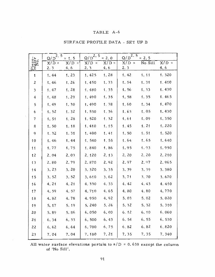
TABLE A-6

SURFACE PROFILE DATA - SET UP B

---'-I;.. QI D2. 5 = 1. 5 QI D2. 5 = 2.0 QI D2 . 5 = 2. 5 o .

N<l)O X/D = X/D = X/D X/D X/D = No Sill X/D <l)~

P:S 2. 3 4.6 2.3 4. 6 2.3 4.6

1 1. 44 1. 23 1.425 1. 28 1. 42 1.11 1.320

2 1. 46 1. 26 1. 450 1. 33 1. 54 1. 31 1. 410

3 1. 47 1. 28 1.480 1. 35 1. 56 1. 33 1.430

4 1. 48 1. 29 1.490 1. 35 1. 58 1. 35 1.465

5 1. 49 1. 30 1.490 1. 38 1. 60 1. 34 1. 470

6 1. 52 1. 32 1. 530 1. 36 1. 63 1. 05 1. 430

7 1. 51 1. 28 1. 520 1. 32 1. 61 1. 09 1.350

8 1. 50 1. 18 1. 410 1. 15 1. 45 1. 21 1.220

9 1. 32 1. 31 1. 400 1. 41 1. 50 1. 51 1. 520

10 1. 46 1. 44 1. 540 1. 55 1. 64 1. 65 1. 640

11 1. 77 1. 75 1. 840 1. 86 1. 95 1. 93 1.950

12 2. 04 2.03 2.120 2. 13 2. 20 2. 20 2. 210

13 2. 80 2. 79 2. 870 2.92 2.97 2.97 2.965

14 3. 23 3. 20 3. 320 3. 35 3.39 3. 39 3.380

15 3. 52 3.52 3. 610 3. 62 3.71 3. 70 3. 670

16 4.21 4. 21 4. 330 4. 33 4.42 4.43 4.410

17 4. 59 4.57 4.710 4. 65 4. 80 4.80 4.770

18 4.82 4. 78 4.950 4.92 5.03 5.02 5. 020

19 5.17 5.19 5.240 5.26 5.32 5.32 5.310

20 5. 89 5.86 6.050 6.00 6. 12 6. 10 6. 060

21 6. 34 6.33 6.500 6.43 6.54 6. 55 6.530

22 6. 62 6.64 6. 700 6,75 6. 82 6. 82 6.820

23 7.04 7.04 7.180 7. 21 7.35 7. 35 7.340

All water surface elevations pertain to siD O. 638 except the column of 'No Sill'.

91

TABLE A-7

SURFACE PROFILE DATA - SET UP B

'I-< Q/D2

. 5 = 3. 00 Q/D2

. 5 = 3.50 Q/.p2.5 00) • = .0 N....,O

X/D = X/D = No Sills X/D = X/D = No Sills X/D = ~f 2.3 4. 6 2.3 4. 6 4. 6

1 1. 53 1. 36 1. 21 1. 57 1. 43 1. 28 1. 530

2 1. 59 1. 48 1. 42 1. 65 1. 57 1. 53 1.650

3 1. 64 1. 52 1. 46 1. 67 1. 59 1. 58 1.670

4 1. 66 1. 55 1. 52 1. 71 1. 64 1. 50 1. 720

5 1. 68 1. 58 1. 54 1. 76 1. 67 1. 63 1. 760

6 1. 79 1. 65 1. 59 1. 87 1. 83 1. 77 1.950

7 1. 79 1. 64 1. 60 1. 91 1. 84 1. 82 1.960

8 1. 75 1.48 1. 35 1. 96 1. 89 1. 83 2. 030

9 1. 52 1. 53 1. 47 1. 97 1. 80 1. 77 2.175

10 1. 62 1. 63 1. 63 1. 93 1. 68 1. 56 2.220

11 1.95 1. 97 1. 95 1. 85 1. 80 1. 80 2. 350

12 2.16 2.17 2.14 2.05 2. 00 2.05 2. 320

13 2.97 2. 97 2.94 2. 85 2. 82 2. 84 2.610

14 3. 39 3. 37 3.36 3. 29 3.23 3.26 3. 030

15 3.71 3.71 3. 71 3. 58 3. 49 3. 56 3. 310

16 4.40 4.42 4. 40 4.29 4. 21 4. 27 4.050

17 4. 79 4. 76 4.77 4.66 4.58 4. 65 4.420

18 5.02 4. 99 4.99 4.86 4.78 4.88 4. 570

19 5.28 5.30 5. 30 5.14 5. 12 5. 13 4.920

20 6.14 6. 12 6.15 6. 00 5.95 6.00 5.750

21 6. 57 6. 56 6. 58 6.45 6. 42 6.44 6.220

22 6. 87 6. 87 6. 79 6.78 6.72 6.73 6. 530

23 7. 35 7.34 7.34 7.24 7. 25 7.24 7.050

All water surface elevations pertain to s / D = O. 638 except the column of 'No Sills. I

92

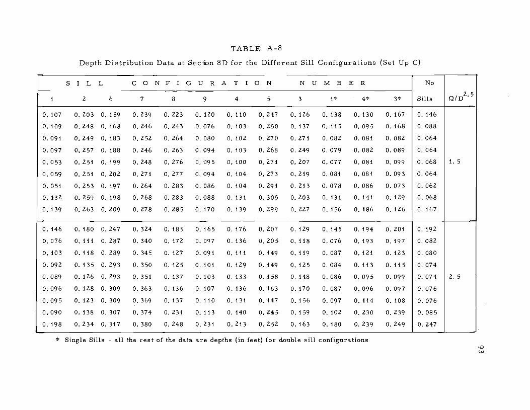
TABLE A-8

Depth Distribution Data at Section 8D for the Different Sill Configurations (Set Up C)

S I L L C 0 N F I G U R A T I 0 N N U M B E R No

1 2 6 7 8 9 4 5 3 1* 4* 3* Sills Q/D2• 5

O. 107 O. 203 O. 159 O. 239 O. 223 O. 120 0.110 O. 247 O. 126 O. 138 0.130 O. 167 0.146

0.109 0.248 O. 168 O. 246 O. 243 0.076 O. 103 O. 250 0.137 0.115 0.095 O. 168 O. 088

0.091 0.249 O. 183 0.252 O. 264 O. 080 O. 102 0.270 0.271 0.082 O. 081 O. 082 0.064

0.097 0.257 O. 188 O. 246 O. 263 O. 094 O. 103 O. 268 O. 249 0.079 O. 082 0.089 O. 064

0.053 O. 251 O. 199 O. 248 O. 276 0.095 O. 100 0.271 0.207 0.077 O. 081 0.099 O. 068 1.5

0.059 0.251 O. 202 0.271 0.277 0.094 O. 104 0.273 0.219 0.081 0.081 0.093 0.064

0.051 0.253 O. 197 0.264 O. 283 O. 086 O. 104 O. 291 0.213 0.078 O. 086 0.073 O. 062

0.132 0.259 O. 198 0.268 O. 283 0.088 O. 131 O. 305 0.203 0.131 0.141 o. 129 O. 068

0.139 0.263 O. 209 0.278 0.285 O. 170 0.139 O. 299 O. 227 O. 156 O. 186 O. -126 O. 167

O. 146 O. 180 0.247 O. 324 O. 185 O. 165 O. 176 O. 207 O. 129 0.145 0.194 O. 201 O. 192

0.076 O. 111 O. 287 O. 340 0.172 0.OQ7 O. 136 0.205 0.118 0.076 O. 193 O. 197 O. 082

O. 103 0.118 O. 289 0.345 O. 127 0.091 O. 111 0.149 0.119 O. 087 O. 121 O. 123 O. 080

0.092 O. 135 0.293 O. 350 O. 125 O. 101 O. 129 0.149 O. 125 O. 084 0.113 0.115 O. 074

0.089 O. 126 0.293 O. 351 0.137 O. 103 0.133 O. 158 0.148 O. 086 0.095 O. 099 O. 074 2. 5

0.096 o. 128 0.309 O. 363 O. 136 O. 107 0.136 o. 163 0.170 O. 087 o. 096 O. 097 0.076

0.095 O. 123 0.309 O. 369 0.137 0.110 O. 131 0.147 O. 156 O. 097 0.114 O. 108 O. 076

0.090 O. 138 0.307 O. 374 0.231 0.113 O. 140 0.245 O. 159 O. 102 O. 230 O. 239 0.085

O. 198 0.234 O. 317 O. 380 O. 248 0.231 0.213 0.252 O. 163 O. 180 O. 239 O. 249 O. 247

* Single Sills - all the rest of the data are depths (in feet) for double sill configurations

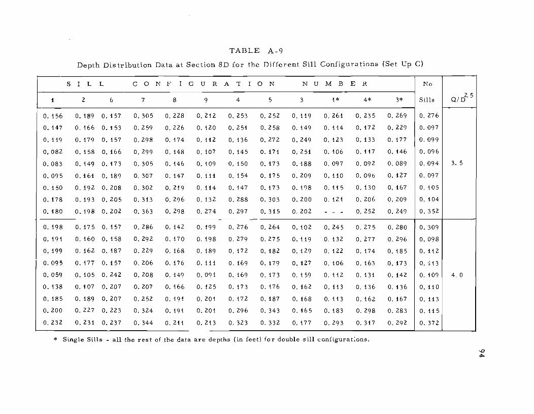
TABLE A-9

Depth Distribution Data at Section 8D for the Different Sill Configurations (Set Up C)

, S I L L C 0 N F I G U R A T I 0 N N U M B E R No

1 2 6 7 8 9 4 5 3 1* 4* 3* Sills Q/ D2. 5

O. 156 O. 189 O. 157 O. 305 O. 228 0.212 O. 253 0.252 0.119 O. 261 0.235 O. 269 0.276

0.147 O. 166 O. 153 0.259 0.226 O. 120 O. 251 0.258 0.149 0.114 0.172 O. 229 O. 097

0.119 0.179 O. 157 O. 298 0.174 0.112 0.136 O. 272 O. 249 O. 123 0.133 0.177 O. 099

0.082 0.158 O. 166 O. 299 O. 148 O. 107 0.145 0.171 0.251 O. 106 0.117 0.146 O. 096

0.083 0.149 O. 173 O. 305 0.146 O. 109 O. 150 O. 173 O. 188 O. 097 0.092 O. 089 0.094 3. 5

0.095 0.161 O. 189 O. 307 0.147 O. 111 O. 154 0.175 O. 209 0.110 O. 096 O. 127 O. 097

O. 150 0.192 O. 208 O. 302 O. 219 0.114 O. 147 O. 173 O. 198 0.115 0.130 O. 167 O. 105

0.178 0.193 0.205 0.313 0.296 0.132 O. 288 O. 303 O. 200 O. 121 O. 206 O. 209 0.104

O. 180 0.198 O. 202 O. 363 0.298 O. 274 O. 297 O. 315 O. 202 - - - O. 252 O. 249 O. 352

O. 198 0.175 O. 157 O. 286 0.142 O. 199 O. 276 O. 264 O. 102 0.245 O. 275 O. 280 0.309

O. 191 0.160 O. 158 0.292 O. 170 O. 198 O. 279 0.275 0.119 O. 132 0.277 O. 296 O. 098

O. 199 O. 162 O. 187 O. 229 O. 168 O. 189 0.172 O. 182 O. 129 O. 122 O. 174 O. 185 0.112

0.095 0.177 O. 157 O. 206 0.176 O. 111 O. 169 O. i 79 O. 127 O. 106 O. 163 0.173 O. i13

0.059 O. 105 O. 242 O. 208 0.149 0.091 O. 169 0.173 O. 159 0.112 0.131 0.142 O. 109 4. 0

0.138 0.107 O. 207 O. 207 O. 166 O. 125 0.173 O. 176 O. 162 0.113 0.136 0.136 0.110

O. 185 O. 189 O. 207 0.252 O. 191 O. 201 0.172 O. 187 O. 168 O. 113 O. 162 O. 167 0.113

0.200 O. 227 O. 223 O. 324 O. 191 0.201 0.296 O. 343 O. 165 O. 183 O. 298 O. 283 0.115

0.232 0.231 O. 237 O. 344 0.211 0.213 O. 323 O. 332 0.177 O. 293 0.317 O. 292 0.372

* Single Sills - all the rest of the data are depths (in feet) for double sill configuraLons.

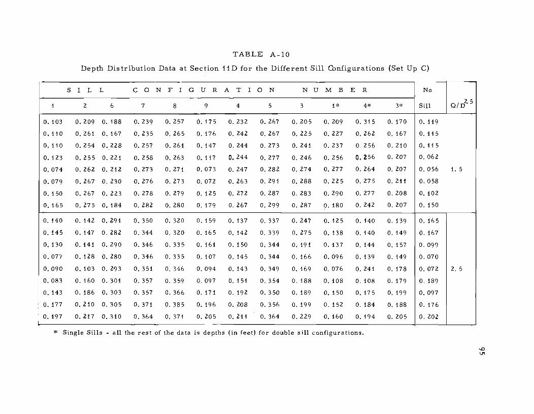
TABLE A-10

Depth Dis tribution Data at Section 11 D for the Different Sill Configurations (Set Up C)

S I L L C 0 N F I G U R A T I 0 N N U M B E R No

1 2 6 7 8 9 4 5 3 1* 4* 3'~ Sill Q/d .. 5

O. 103 0.209 O. 188 O. 239 O. 257 O. 175 O. 232 O. 267 0.205 O. 209 O. 315 0.170 0.119

0.110 0.261 O. 167 0.235 O. 265 O. 176 0.242 O. 267 O. 225 O. 227 0.262 O. 167 0.115

0.110 0.254 O. 228 0.257 0.261 O. 147 O. 244 O. 273 O. 241 O. 237 0, 256 O. 210 0.115

O. 123 0.255 O. 221 0.258 O. 263 O. 117 O. 244 0.277 O. 246 0.256 O. 256 O. 207 O. 062

0.074 O. 262 O. 212 0.273 0.271 0.073 O. 247 O. 282 O. 274 O. 277 O. 264 0.207 O. 056 1. 5

0.079 O. 267 O. 230 0.276 O. 273 O. 072 O. 263 O. 291 O. 288 O. 225 O. 275 O. 211 O. 058

0.150 O. 267 O. 223 O. 278 O. 279 O. 125 0.272 O. 287 O. 283 O. 290 O. 277 O. 208 O. 102

O. 165 0.275 O. 184 O. 282 O. 280 O. 179 O. 267 O. 299 0.287 O. 180 O. 242 O. 207 O. 150

0.140 O. 142 0.291 0.350 O. 320 O. 159 0.137 O. 337 O. 247 O. 125 0.140 O. 139 O. 165

0.145 0.147 O. 282 O. 344 O. 320 O. 165 0.142 O. 339 O. 275 0.138 0.140 0.149 O. 167

0.130 0.141 O. 290 O. 346 0.335 O. 161 O. 150 O. 344 O. 191 0.137 0.144 O. 157 O. 099

0.077 0.128 O. 280 O. 346 0.335 O. 107 0.145 O. 344 O. 166 O. 096 O. 139 O. 149 O. 070

0.090 O. 103 0.293 0.351 O. 346 0.094 0.143 O. 349 O. 169 O. 076 O. 241 O. 178 0.072 2. 5

0.083 O. 160 O. 301 0.357 0.359 O. 097 O. 151 O. 354 O. 188 O. 108 0, 108 O. 179 0, 189

0.143 O. 186 O. 303 O. 357 O. 366 0.171 O. 192 0.350 O. 189 O. 150 O. 175 O. 199 O. 097

0.177 0.210 O. 305 O. 371 0.385 O. 196 0.208 0.356 O. 199 O. 152 0.184 O. 188 O. 176

O. 197 0.217 O. 310 O. 364 O. 371 0.205 0.211 O. 364 O. 229 O. 160 O. 194 O. 205 0.202

* Single Sills - all the rest of the data is depths (in feet) for double sill configurations.

TABLE A-ll

Depth Dis tribution Data at Sec tion 11 D for the Different Sill Configurations (Set Up C)

S I L L C 0 N F I G U R A T I 0 N N U M B E R No

1 2 6 7 8 9 4 5 3 1* 4* 3* Sills Qf D2. 5

0.195 0.184 O. 189 O. 373 O. 207 O. 187 O. 197 0.177 0.177 O. 189 0.178 O. 180 0.205

0.186 0.178 O. 187 O. 360 O. 207 O. 200 O. 186 O. 190 0.210 0.177 O. 169 0.178 O. 183

0.158 0.172 O. 183 O. 362 0.251 0.172 O. 191 O. 193 0.215 O. 156 O. 175 O. 179 O. 086

0.113 O. 169 0.177 O. 368 O. 371 O. 160 O. 189 O. 227 O. 211 0.163 O. 161 0.176 0.084 '-

0.092 O. 129 O. 213 O. 374 0.371 0.097 O. 193 O. 286 0.258 0.095 O. 153 O. 251 0.086 3. 5

0.140 O. 225 O. 210 O. 379 O. 378 O. 121 O. 222 O. 265 O. 262 O. 160 O. 166 O. 211 O. 084

0.190 0.252 O. 209 O. 366 O. 263 O. 180 O. 225 O. 239 O. 258 O. 190 O. 191 O. 207 0.092

0.220 0.256 O. 240 O. 363 O. 249 0.218 O. 231 O. 251 O. 261 O. 215 O. 203 O. 234 O. 238

0.228 0.258 O. 251 0.433 O. 242 O. 224 0.245 O. 256 O. 255 O. 230 O. 204 0.235 O. 256

0.229 O. 192 O. 189 O. 427 0.201 O. 227 0.221 O. 226 O. 181 O. 229 0.213 O. 194 0.247

0.227 0.200 O. 18<) 0.412 0.220 O. 229 O. 221 O. 226 O. 199 0.226 O. 212 0.207 O. 235

0.202 0.201 O. 192 0.416 O. 229 0.210 0.228 O. 225 O. 209 O. 182 O. 210 O. 204 0.095

O. 109 0.177 O. 187 0.416 O. 237 O. 121 O. 219 O. 220 O. 206 O. 138 0.205 O. 191 0.095

0.087 0.141 O. 279 0.423 O. 201 O. 101 O. 332 O. 318 O. 239 0.085 O. 195 O. 307 0.096 4. 0

0.165 O. 149 O. 234 0.425 O. 223 O. 167 O. 273 O. 262 O. 243 O. 186 0.247 O. 226 O. 102

O. 230 0.249 O. 232 O. 439 O. 241 O. 236 O. 270 0.271 O. 249 O. 220 O. 243 0.247 O. 102

0.250 0.264 O. 253 0.431 O. 237 0.259 0.275 O. 286 O. 262 O. 250 O. 249 O. 252 0.272

0.260 0.271 O. 261 0.444 0.275 O. 239 O. 268 O. 291 0.259 O. 263 O. 252 0.245 O. 280

* Single Sills - are all the rest of the data depths (in feet) for double sill configurations

Table A-12. Surface Profile Data from Set Up D

Station Q/D2

.5 = 1.5 2. 5 3. 5 6. 0

Number D E P T H S I N F E E T

* ,.~* * ** * ** * ** 1 0.403 O. 384 0.495 - - - - 0.573 - - - - O. 804 - - - -

2 .390 .376 .456 - - - - .546 - - - - .790 - - - -

3 .394 .382 .453 0.463 .565 O. 595 .798 O. 800

4 .388 .405 .446 .450 · 551 . 575 .812 .801

5 .372 .406 .440 .458 .536 .572 .840 .835

6 .401 .394 .479 .462 .572 .607 .888 .862

7 .417 .388 .483 - - - - .566 .627 .867 .867

8 .400 .389 .498 - - - - .570 .620 .827 .838

9 .405 .363 .475 - - - - .596 .616 .794 .809

10 .393 . 373 .482 - - - - .592 .620 .808 . 818

11 . 371 .375 .458 - - - - · 583 . 598 .839 .847

12 .393 - - - - .450 - - - - · 575 .604 .865 .875

13 .390 - - - - .439 - - - - .580 - - - - .848 .846

14 .385 - - - - .416 - - - - .564 - - - - .793 - - - -

15 .367 - - - - .484 - - - - .596 - - - - .793 - - - -

16 .400 - - - - .488 - - - - · 558 - - - - .837 - - - -17 .386 - - - - .479 - - - - .596 - - - - .811 - - - -

18 .426 - - - - .468 - - - - .613 - - - - .849 - - - -

19 .414 - - - - .412 - - - - .610 - - - - .859 - - - -20 .437 - - - - .572 - - - - .626 - - - - .859 - - - -21 .442 - - - - .577 - - - - .652 - - - - .969 - - - -22 .511 - - - - .672 - - - - .704 - - - - - - - - - - - -23 .658 - - - - .696 - - - - - - - - - - - - - - - - - - - -

* No Sills

** No Sills (Repeated Data)

97

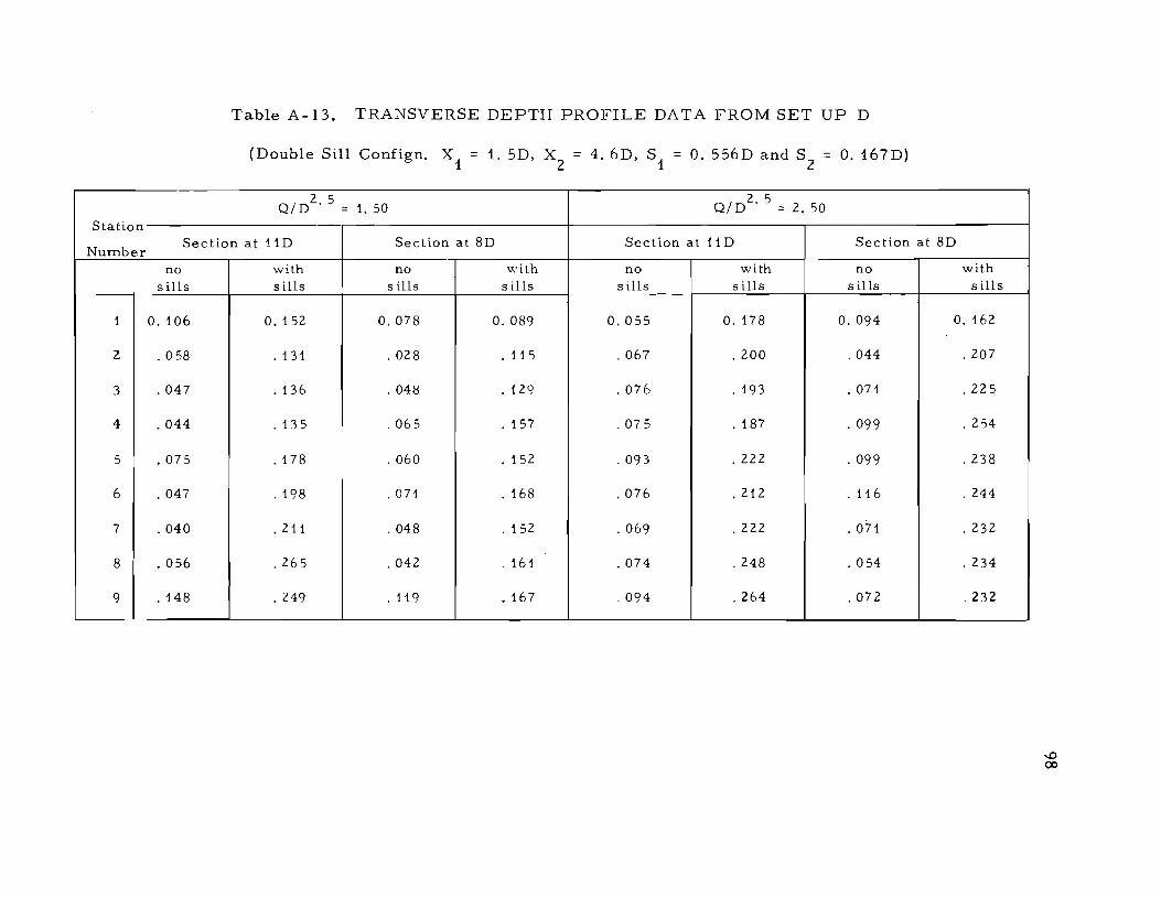
Table A-13. TRANSVERSE DEPTH PROFILE DATA FROM SET UP D

(Double Sill Confign. X ::: 1. 5D, X ::: 4. 6D, S ::: O. 556D and S ::: O. 167D) 1 2 1 2

Q/D2

.5 = 1. 50 Q/D

2.

5 = 2. 50 Station

NUTIlber Section at 11 D Section at 8D Section at 11 D Section at 8D

no with no with no with no with

sills sills sills sills sills sills sills sills

1 O. 106 0.152 0.078 O. 089 0.055 O. 178 O. 094 O. 162

2 .058 · 131 .028 .115 .067 .200 .044 · 207

3 .047 .136 .04i:l · 12q .076 · 193 .071 .225

4 .044 · 135 .065 · 157 .075 · 187 .099 · 254

5 .075 .178 .060 · 152 .093 · 222 .099 .238

6 .047 · 198 . 071 · 168 .076 · 212 .116 .244

7 .040 .211 .048 · 152 .069 .222 .071 · 232

8 .056 .265 .042 ,161 .074 .248 .054 · 234

9 . 148 .249 .119 · 167 ,094 .264 .072 · 232

Table A-14. TRANSVERSE DEPTH PROFILE DATA FROM SET UP D

(Double Sill Confign. Xi = 1. 5D, X2 = 4. 6D, S1 = O. 556D and S2 = O. 167D)

Q/D2

• 5 = 3.50 Q/D2. 5 = 6.00 I

Station I Number

Section at 11D Section at 8D Section at 11 D Section at 8D

no with no with no with no with sills sills sills sills sills sills sills sills

1 0.207 0.176 0.066 O. 204 - - - - O. 351 0.064 - - - -

2 .076 .200 .048 .209 0.098 .342 .060 - - - -

3 .073 .203 .078 .218 .099 .328 .111 - - - -

4 .066 .218 .113 .245 .096 .318 .142 - - - -

5 0095 ,261 . 105 ,236 .122 .346 . 145 - - - -

6 .072 .253 . 108 .232 .102 .332 .138 - - - -

7 .071 .263 .088 .219 ~

. 101 .343 .113 - - - -

8 .076 .255 .070 .234 .106 .352 .095 - - - -

9 .287 .230 .076 .238 - - - - .354 . 101 - - - -

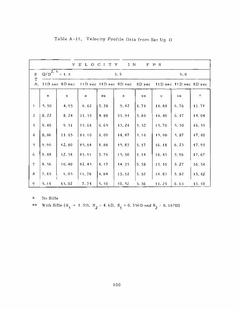
Table A-15. Velocity Profile Data from Set Up D

V E L 0 C I T Y I N F P S

S Q/D2. 5 = 1. 5 3. 5 6. 0 T A. 11D sec 8D sec 11D sec 11D sec 8D sec 8D sec 11 D sec 11 D sec 8D sec

* ~I::; ~~ ** .. ** :::;,; ** -'--0

1 5. 50 4.95 6.62 5. 38 9.42 4.74 11. 88 6.76 11. 71

2 8. ZZ 8.24 11.33 4. 88 11. 94 5. 84 14. 40 6.47 14. 04

3 9.46 9. 31 13. 64 4.65 13. 24 5. 52 15.70 5. 30 16. 35

4 8.86 11. 15 13. 10 4. 09 14.87 5. 14 15.90 5. 87 17.40

5 9.96 12. 80 15.14 4. 88 15.83 5.17 16. 18 6. 23 17.95

6 9.48 12. 34 13.91 3.76 15. 50 5. 14 16.43 5.96 17.67

7 8,56 10.40 12.45 4.17 14. 35 5. 38 15. 10 5. Z7 16. 54

8 7.45 9.05 11. 78 4. 84 13. 12 5. 52 14. 83 5. 82 15.42

9 5.14 15. 02 7.74 5. 10 10. 52 5. 36 11. 25 6. 63 13. 10

~~ No Sills

** With Sills (Xi 1.5D, X2

= 4. 6D, S1 = O. 556D and S2 = O. 167D)

100

Table A-16. Surface Profile Data from Set Up E

Station Q/D2

. 5= 1.5 2.5 3. 5 6. 0

Number D E P T H S I N F E E T

* ** * ** * ** * ** 1 0.412 1. 007 0.532 - - - - O. 624 - - - - p. 850 - - - -2 .423 .989 .552 - - - - .649 1. 025 . 851 - - - -3 .431 .756 · 564 0.491 · 661 .731 .852 0.906 4 .426 .431 · 561 .511 .630 .641 .835 .848 5 .397 .396 .545 .509 .624 .628 .840 .980 6 .399 .382 · 591 . 507 · 601 · 614 .838 . 819 7 .426 .414 .538 . 514 · 631 .627 .845 .855 8 .413 .413 · 518 .490 .622 .611 .834 .868 9 .396 · 415 · 515 .473 .607 .617 .862 .925

10 .375 .394 · 512 .473 .605 .625 .930 1. 088 11 . 391 · 413 .503 .481 .639 .709 ~. 019 .802 12 .394 .384 · 518 .484 .607 .592 .817 .772 13 .389 .385 · 515 .489 .609 .620 .792 - - - -14 .389 .374 · 512 - - - - .605 - - - - .789 - - - -15 .367 .374 .484 - - - - .584 - - - - .793 - - - -16 .364 .374 .470 .453 .578 · 581 .804 .814 17 .377 .368 · 500 - - - - · 593 - - - - .857 - - - -18 .395 .392 · 539 - - - - .621 - - - - .860 - - - -19 . 391 .378 · 541 - - - - .626 - - - - .834 - - - -20 .385 .387 .527 .498 .618 - - - - .808 - - - -21 .388 .388 · 533 - - - - .602 - - - - .806 - - - -22 .362 .377 .483 - - - - · 581 - - - - .791 - - - -23 .375 · 361 · 509 - - - - .587 - - - - .839 - - - -24 .374 .370 · 513 - - - - · 579 - - - - .826 - - - -25 .374 .386 · 519 .472 .623 - - - - .790 - - - -26 .387 · 381 .507 - - - - · 641 - - - - .842 - - - -27 .402 .415 .546 .504 · 599 · 597 .833 .879 28 .433 .426 .508 - - - - .631 - - - - .844 - - - -29 .425 .416 · 521 - - - - .664 - - - - .888 - - - -30 .390 .375 .528 .530 .654 - - - - .833 - - - -31 .419 .410 .607 - - - - .669 - - - - .857 - - - -32 .454 .434 .644 .635 · 681 - - - - .949 - - - -33 .543 · 515 .699 - - - - .752 - - - - . 108 - - - -34 .623 .590 .713 - - - - .844 - - - - - - - - - - -

-

* No Sills

** With Sills (Xi = 1. 5D, X2 = 4. 6D, S1 = O. 5D, S2 = o. 167D)

101

Station

Number

1

2

3

4

5

6

7

8

9

Table A-I7. TRANSVERSE DEPTH PROFILE DATA FROM SET UP E

(Double Sill Confign. Xi:::: 1. 5D, X2

:::: 4. 6D, S 1 :::: O. 5D, and S2 :::: O. 167 D)

Q/D2. 5 = 1. 50 Q/D2

.5 = 2.50 Q/D

2. 5 = 3. 50 Q/D2. 5 = 6.0

Section at 8D Section at 8D Section at 8D Section at 8D

no with no with :10 with no with sills sills s [lls sills sills sills sIlls sills

O. 101 0.148 0.159 O. 196 O. 120 O. 233 O. 105 O. 303

.052 .150 .062 .200 .068 .231 .090 · 350

.068 .148 .087 · 199 .095 .233 .117 · 353

.068 . 129 . 100 · 185 · 100 .220 .130 .340

.076 .102 .111 · 187 .114 .240 · 148 · 354

.07 i .119 .115 · 188 · 103 .251 · 129 · 343

.063 .134 .089 · 191 .079 .248 .114 · 335

.052 .143 .078 .206 .070 .261 .097 · 355

. 153 . 166 . 184 .203 · 123 .247 · 123 .360

.... o N

Table A-18. Velocity Profile Data from Set Up E

V E L 0 C I T Y I N F P S

S Q/D2. 5 = 1. 5 3. 5 6.0 T A. 8D Sec 8D Sec 8D Sec 8D Sec 8D Sec 8D Sec

-,- ......... 1 ... -'- ** * ** -,' .......... r- -,-

1 4. 58 3, 16 8. 49 4.35 12.09 5. 12

2 7.31 3. 16 10. 30 4.32 13.68 5. 10

3 9.04 2.98 12.20 4.58 15.00 6.37

4 9. 57 3.04 13.07 4.65 15.48 7. 13

5 11. 15 3.72 14. 18 4. 65 15.88 8.34

6 10.38 3. 42 13. 57 4. 51 15.71 7.71

7 9.10 3.63 13. 10 4.30 14. 41 6. 89

8 8.45 3. 68 11. 88 4. 43 13. 87 6. 00

9 4.96 3. 31 9.93 4.47 12. 12 5. 46

* No Sills

With Sills (X1

= 1. 5D, X2

= 4. 6D, S 1 = O. 5D, and S2 = O. 167 D)

103

Table A 19. Surface Profile Data from Set Up F

Sta tion QID2

. 5 1.5 2. 5 3. 5 6. 0

Number D E P T H S I N F E E T

oJ,

** !i:: *:..\: * ** * ** -0-

1 0.385 1. 011 0.481 - - - - O. 569 - - - - O. 767 - - - -2 .416 .903 · 523 0.972 . 585 0.992 .775 - - - -3 .410 .659 · 532 . 577 .580 .902 .816 0.906

4 .417 .356 .544 .490 .662 .613 .896 .884

5 .418 . 351 · 551 .522 .726 .603 .934 .870

6 .416 .397 .485 .485 .606 · 599 .787 .769

7 .391 .339 .483 .466 .612 · 593 .840 .773

8 .356 .339 · 523 .496 . 564 · 555 .799 .796

9 .384 .361 · 512 .491 .619 · 598 .843 .799

10 .414 .404 .482 .486 .653 .627 .854 .847

11 .440 .434 · 530 .533 .661 .667 .855 .870

12 .463 .470 .588 . 582 .650 .668 - - - - - - - -13 . 526 . 529 .656 .652 .725 .703 - - - - 1.071

14 .589 .584 .703 .713 .852 .787 - - - - - - - -

* No Sills

** With Sills (X1

:;; 1. 5D, X2

::: 4. 6D, S1 = O. 556D and S2 0.167D)

104

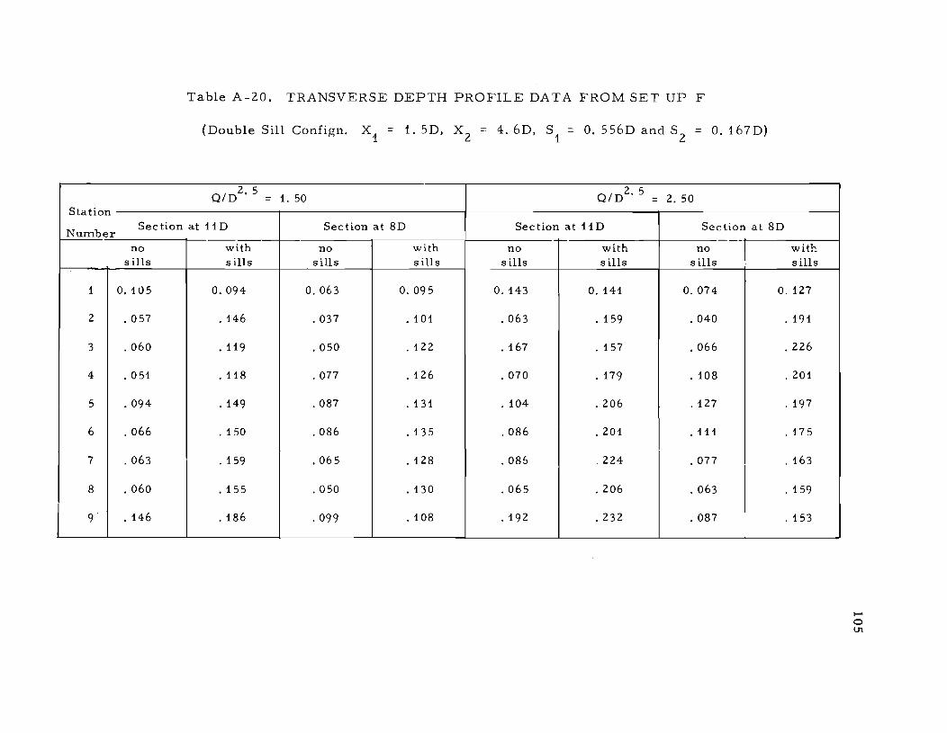
Station

Number

1

2

3

4

5

6

7

8

9

Table A-20. TRANSVERSE DEPTH PROFILE DATA FROM SET UP F

(Double Sill Confign. Xi = 1. 5D, Xz

= 4.6D, S1 = O. 556D and Sz = O.167D)

QID2. 5 = 1. 50 QID2. 5 = 2.50

Sec tion at 11 D Section at 8D Section at 11D Section at 8D

no with no with no with no witr.. sills sills sills sills sills sills sills 5 ills

0.105 0.094 0.063 0.095 O. 143 O. 141 0.074 O. 127

.057 .146 .037 · 101 .063 · 159 .040 · 191

.060 .119 .050 · 122 · 167 · 157 .066 .226

.051 .118 .077 · 126 .070 .179 . 108 · 201

.094 .149 .087 · 131 · 104 .206 . 127 · 197

.066 . 150 .086 .135 .086 · 201 .111 · 175

.063 .159 .065 · 128 .086 .224 .077 · 163

.060 .155 .050 .130 .065 .206 .063 · 159

. 146 .186 .099 · 108 · 192 .232 .087 · 153

-o U1

Table A-Zl. TRANSVERSE DEPTH PROFILE DATA FROM SET UP F

(Double Sill Confign. Xi = 1. 5D, Xz

= 4. 6D, S 1 = O. 556D and Sz = O. 167 D)

QfD2

• 5 3.50 Qf D2. 5 :: 6.00

Station

Number Section at 11D Section at 8D Sec Hon at 11 D Section at 8D

no with no with no with no with sills sills sills sills sills sills sills sills

1 O. 190 O. 183 0.049 O. 200 O. 322 0.280 0.113 - - - -

2 .075 . 193 . 061 .230 · 105 .261 .080 - - - -

3 .083 .217 .087 .275 .111 .273 .115 - - - -

4 . 105 .212 .118 .278 · 126 . 281 .134 - - - -

5 .130 .237 , 141 .282 .146 .296 .148 - -

6 .111 .240 . 127 .261 .134 .297 .133 - - - -

7 .091 .249 .098 .229 .116 .306 .117 - - - -

8 .098 .244 .080 .224 .117 .307 .091 - - - -

9 .253 .230 ,078 .220 · 363 .295 .196 - - - -

-o 0'

Table A-22. Velocity Profile Data from Set Up F

V E L 0 C I T Y I N F P S

S Q/ D2. 5 ::: 1. 5 2. 5 3. 5 T

A 11Dsec 11 D sec 11D sec 11D sec 11 D sec 11 D sec

,C

** * ** * ** ....

i 4. 87 3. 25 6. 20 3.72 7.22 4.36

2 7. 23 3. 52 9.25 4. 02 11. 15 4. 30

3 8.17 3. 25 10. 35 3.48 12. 20 4. 06

4 8. 47 3.07 11. 25 3.46 13.45 3.73

5 10. 15 2. 55 12. 35 3.17 13. 58 3. 50

6 8. 20 2. 78 10.78 3. 25 12. 55 3.77

7 8.80 2. 86 11. 46 3.72 13.40 3.94

8 7.92 2. 86 10.40 3.96 12.90 4.39

9 4.86 2.72 7.08 3. 62 6. 50 4. 35

* No Sills .. 1... ... 1 .. TO'I" With Sills (Xi::: 1. 5D, X

2 = 4. 6D, S1 ::: O. 556D, S2 = O. 167D)

107

6. 0

1iD sec 11Dsec

* ** 12. 30 6. 56

14.80 5. 44

I 16. 00 5.60

15.25 4. 68

17. 35 5. 23

15. 50 4.94

15. 80 5.54

13.90 5.54

10.95 5. 74

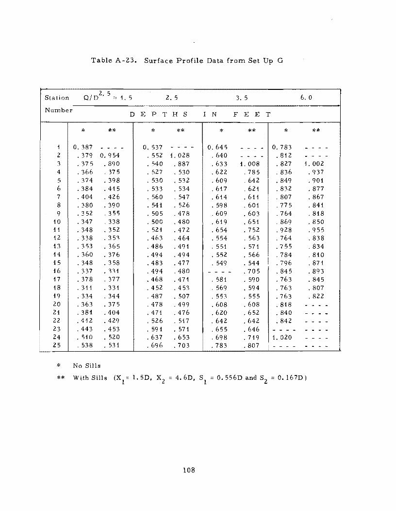
Table A-23. Surface Profile Data from Set Up G

Sta tion Q/ D2. 5 ::: 1. 5 2. 5 3. 5 6.0

Number D E P T H S I N F E E T

* ** * *'" '" "'''' '" *'" 1 O. 387 - - - - 0.537 - - - - 0.645 - - - - 0.783 - - - -2 .379 0.954 · 552 1. 028 .640 - - - - . 812 - - - -3 .375 .890 .540 .887 .633 1.008 .827 1. 002 4 .366 .375 .527 .530 .622 .785 .836 .937 5 .374 .398 · 530 .532 .609 .642 .849 .901 6 .384 .415 .533 .534 .617 .621 .832 .877 7 .404 .426 · 560 .547 .614 .611 .807 .867 8 .380 .390 · 541 .526 .598 .601 .775 .841 9 .352 .355 · 505 .478 .609 .603 .764 .818

10 .347 .338 .500 .480 .619 · 651 .869 .850 11 .348 · 352 · 521 .472 .654 .752 .928 .955 12 .338 .353 .463 .464 .554 · 563 .764 .838 13 .353 .365 .486 .491 · 551 · 571 .755 .834 14 .360 .376 .494 .494 · 552 .566 .784 .810 15 .348 .358 .483 .477 .549 .544 I .796 .871 16 .337 · 331 .494 .480 - - - .705 .845 .893 17 .378 .377 .468 .471 · 581 · 590 .763 .845 18 .311 · 331 .452 .453 · 569 .594 .763 .807 19 .334 .344 .487 .507 .553 · 555 .763 .822 20 .363 .375 .478 .499 .608 .608 .818 - - - -21 .381 .404 .471 .476 .620 .652 .840 - - - -22 .412 .429 .526 .517 .642 .642 .842 - - - -23 .443 .453 · 591 . 571 .655 .646 - - - - - - - -24 . 510 · 520 .637 .653 .698 · 719 1. 020 - - - -25 .538 · 531 .696 .703 .783 .807 I - - - - - - -

* No Sills

** With Sills (Xl = 1. 5D, X2 = 4.6D, SI O. 556D and S2 = O. 167D)

108

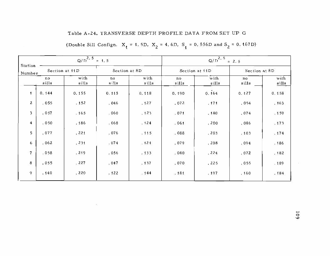
Station

Number

1

2

3

4

5

6

7

8

9

Table A-Z4. TRANSVERSE DEPTH PROFILE DATA FROM SET UP G

(Double Sill Confign. X1

= 1. 5D, Xz

= 4. 6D, S 1 = O. 556D and Sz = O. 167 D)

Qf D2. 5 = 1.5 Qf D2, 5 = 2. 5

Sec tion at 11 D Section at 8D Section at 11D Sec tion at 8D

no with no with no with no with sills sills sills sills sills sills sills sills

0.144 O. 155 0.115 0.118 O. 190 O. 164 O. 127 O. 158

.055 · 152 .046 .127 .072 · 171 .054 · 163

.057 · 165 .060 · 123 .071 · 180 .074 · 159

.050 · 186 .068 · 124 .061 .200 .086 .173

.077 .221 .076 .115 .088 .203 . 103 · 174

.062 · 231 .074 · 124 .079 .208 .094 · 186

,058 .219 .056 .133 .080 .224 .072 · 182

.055 .227 .047 · 137 .070 · 225 .055 , 189

.140 .220 . 122 .144 . 181 · 197 . 160 · 184

-o ..0

1

2

3

4

5

6

7

8

9·

Table A-25. TRANSVERSE DEPTH PROFILE DATA FROM SET UP G IN FEET

(Double Sill Configuration X1

= 1. 5D, X2

4. 6D, S1 = O. 556D and S2 = O. 167D)

. Q/ 2.5 D = 3.5 Q/ D2. 5 = 6.0

Section at 11 D Section at 8D Section at 11D Section at 8D

no sills with sills no sills with sills no sills with sills no sills with sills

u,2.38 0, 201 O. 073 0. ~O1 0.215 0.275 CJ. 102 - - - -

O. 079 0.212 0.072 0.222 O. 102 O. 279 0.104 - - - -

O. 083 0.213 0.092 0.199 0.117 0.271 0.133 - - - -

0.082 O. 266 O. 102 0.189 0.122 0.298 0.142 - - - -

O. 108 O. 271 0.113 O. 203 0.137 O. 281 O. 160 - - - -

O. 100 O. 273 O. 113 O. 202 0.131 O. 279 O. 156 - - - -

O. 100 o. 249 0.089 0.213 O. 133 O. 288 O. 128 - - - -

0.880 O. 230 O. 070 O. 239 O. 131 0.301 O. 090 - ~ - -0.266 O. 223 0.088 O. 220 O. 331 0.283 0.175 - - - -

..... ..... o

S T A.

1

2

3

4

5

6

7

8

9

* **

Table A-26. Velocity Profile Data From Set Up G

V E L 0 C I T Y I N F P S

Q/D2. 5 = 1. 5 2.5 3. 5

~!~ ** ,.~ ** * >:'* ~;:

5. 51 3.17 6.73 3. 80 6. 97 4.73 11. 30

7.63 3. 38 9. 15 3. 68 11. 50 4. 29 13.87

8. 39 3. 25 10. 26 3.06 12. 55 4. 18 14.50

8.05 2. 88 10. 30 3.11 12. 53 3. 31 15. 10

9.85 2. 70 11. 76 3.00 13. 15 3. 59 14.84

8.90 2. 63 11. 07 3. 19 13.01 3. 55 14.64

8. 21 2. 52 10.79 3.05 12.94 4. 10 14.60

7.84 1. 56 9.64 3. 41 11. 59 4. r:.,7 13. 51

5. 38 2. 71 6. 13 3. 74 6. 83 4. 55 10.47

No Sills

With Sills (Xi = 1. 5D, X z = 4. 6D, S1 = O. 556D and S2 = O. 167D)

All Values at lID Section

111

6.0

*>:'

4.35

5. 10

5.20

5. 57

5. 80

5.36

5.14

5. 36

5. 12 . '"