performance analysis of a closed-cycle ocean thermal

University of Rhode Island University of Rhode Island

DigitalCommons@URI DigitalCommons@URI

Open Access Master's Theses

2013

PERFORMANCE ANALYSIS OF A CLOSED-CYCLE OCEAN PERFORMANCE ANALYSIS OF A CLOSED-CYCLE OCEAN

THERMAL ENERGY CONVERSION SYSTEM WITH SOLAR THERMAL ENERGY CONVERSION SYSTEM WITH SOLAR

PREHEATING AND SUPERHEATING PREHEATING AND SUPERHEATING

Hakan Aydin University of Rhode Island, [email protected]

Follow this and additional works at: https://digitalcommons.uri.edu/theses

Recommended Citation Recommended Citation Aydin, Hakan, "PERFORMANCE ANALYSIS OF A CLOSED-CYCLE OCEAN THERMAL ENERGY CONVERSION SYSTEM WITH SOLAR PREHEATING AND SUPERHEATING" (2013). Open Access Master's Theses. Paper 163. https://digitalcommons.uri.edu/theses/163

This Thesis is brought to you for free and open access by DigitalCommons@URI. It has been accepted for inclusion in Open Access Master's Theses by an authorized administrator of DigitalCommons@URI. For more information, please contact [email protected].

https://digitalcommons.uri.edu/

https://digitalcommons.uri.edu/theses

https://digitalcommons.uri.edu/theses?utm_source=digitalcommons.uri.edu%2Ftheses%2F163&utm_medium=PDF&utm_campaign=PDFCoverPages

https://digitalcommons.uri.edu/theses/163?utm_source=digitalcommons.uri.edu%2Ftheses%2F163&utm_medium=PDF&utm_campaign=PDFCoverPages

mailto:[email protected]

PERFORMANCE ANALYSIS OF A CLOSED-CYCLE

OCEAN THERMAL ENERGY CONVERSION SYSTEM

WITH SOLAR PREHEATING AND SUPERHEATING

BY

HAKAN AYDIN

A THESIS SUBMITTED IN PARTIAL FULFILLMENT OF THE

REQUIREMENTS FOR THE DEGREE OF

MASTER OF SCIENCE

IN

MECHANICAL ENGINEERING AND APPLIED MECHANICS

UNIVERSITY OF RHODE ISLAND

2013

MASTER OF SCIENCE THESIS

OF

HAKAN AYDIN

APPROVED:

Thesis Committee:

Major Professor Keunhan Park

Zongqin Zhang

Seung Kyoon Shin

Nasser H. Zawia

DEAN OF THE GRADUATE SCHOOL

UNIVERSITY OF RHODE ISLAND

2013

ABSTRACT

The research presented in this thesis provides thermodynamic insights on the

potential advantages and challenges of adding a solar thermal collection component

into ocean thermal energy conversion (OTEC) power plants. In that regard, this article

reports the off-design performance analysis of a closed-cycle OTEC system when a

solar thermal collector is integrated as an add-on preheater or superheater into the

system.

The present research aims to examine the system-level effects of integrating solar

thermal collection with an existing OTEC power plant in terms of power output and

efficiency. To this end, the study starts with the design-point analysis of a closed-cycle

OTEC system with a 100 kW gross power production capacity. The numerically

designed OTEC system serves as an illustrative base which lays the ground for

thermodynamic analysis of off-design operation when solar thermal collection is

integrated. Two methods that make use of solar energy are considered in this research.

Firstly, an add-on solar thermal collector is installed in the system in order to preheat

the surface seawater before it enters the evaporator. The second way considered is

directly superheating the working fluid between the evaporator and the turbine with

the add-on solar thermal collector. Numerical analysis is conducted to predict the

change of performance (i.e., net power and efficiency) within the OTEC system when

solar collection is integrated as a preheater/superheater. Simulated results are

presented to make comparison of the improvement of system performance and

required collector effective area between the two methods. In the conclusion, possible

ways to further improve the solar collector efficiency; hence the overall thermal

efficiency of the combined system are suggested.

Obtained results reveal that both preheating and superheating cases increase the

net power generation by 20-25% from the design-point. However, the preheating case

demands immense heat load on the solar collector due to the huge thermal mass of the

seawater, being less efficient thermodynamically. Adverse environmental impacts due

to the increase of seawater temperature are also of concern. The superheating case

increases the thermal efficiency of the system from 1.9 % to ~3%, about 60%

improvement, suggesting that it should be a better and more effective approach in

improving a closed-cycle OTEC system.

iv

ACKNOWLEDGMENTS

All of the work and research presented in this master’s thesis was carried out

under the supervision and guidance of Dr. Keunhan Park at the University of Rhode

Island. It goes without saying that I am very grateful for his support and

encouragement throughout all my work at URI including but not limited to the

submission of a journal paper. I would also like to take the opportunity to thank Dany

for reminding me always to stay positive and focused on my goals. Finally my heart-

felt thanks go to my parents and my sister for their continuous moral and material

support from across the Atlantic.

v

TABLE OF CONTENTS

ABSTRACT .................................................................................................................. ii

ACKNOWLEDGMENTS .......................................................................................... iv

TABLE OF CONTENTS ............................................................................................. v

LIST OF TABLES ..................................................................................................... vii

LIST OF FIGURES .................................................................................................. viii

CHAPTER I: Introduction and Review of Literature ............................................. 1

1.1 Ocean Thermal Energy Conversion ................................................................... 1

1.2 Previous Related Studies .................................................................................... 3

1.3 OTEC System Components ............................................................................... 5

1.3.1 Heat Exchangers ......................................................................................... 6

1.3.2 Pumps .......................................................................................................... 7

1.3.3 Turbine ........................................................................................................ 8

CHAPTER II: Design-Point Analysis of OTEC ...................................................... 11

2.1 Methodology .................................................................................................... 11

2.2 Results and Discussion ..................................................................................... 19

CHAPTER III: Off-Design Performance Analysis of OTEC ................................ 23

3.1 OTEC with Solar Thermal Collection.............................................................. 23

3.2 Solar Preheating of Seawater ........................................................................... 26

3.3 Solar Superheating of Working Fluid .............................................................. 33

3.4 Results and Discussion ..................................................................................... 36

vi

CHAPTER IV: Conclusion ....................................................................................... 39

4.1 Summary of Results and Findings ................................................................... 39

4.2 Recommendations for Further Research .......................................................... 40

APPENDICES ............................................................................................................ 41

Appendix A: REFPROP Matlab Code ................................................................... 41

Appendix B: OTEC Design-Point and Off-Design Analysis Code ....................... 55

BIBLIOGRAPHY ...................................................................................................... 68

vii

LIST OF TABLES

Table Page

Table 2.1 Conditions and assumptions for the design of an OTEC system with 100 kW

gross power generation ............................................................................................... 12

Table 2.2 Various heat transfer correlations in literature that model Nusselt number

and Reynolds number .................................................................................................. 13

Table 2.3 Design-point analysis simulation results for the closed-cycle OTEC system

with 100 kW gross power generation.......................................................................... 20

viii

LIST OF FIGURES

Figure Page

Figure 1.1 Schematic representation of a closed-cycle OTEC system and its

components ................................................................................................................... 1

Figure 1.2 Average ocean temperature differences between the depths of 20 m and

1000 m ........................................................................................................................... 3

Figure 1.3 (a) Schematic diagram of a closed OTEC cycle and its components

(b) T-s diagram of the corresponding cycle .................................................................. 5

Figure 2.1 Change of design mass flow rates of the cold and warm seawater as a

function of the target warm seawater output temperature ........................................... 15

Figure 2.2 Change of design mass flow rates of the cold and warm seawater as a

function of the target cold seawater output temperature ............................................. 16

Figure 2.3 Flowchart of the calculation methodology of the MATLAB code ........... 18

Figure 2.4 Turbine isentropic efficiency as a function of shaft rotational speed under

design-point conditions ............................................................................................... 21

Figure 3.1 Collector thermal efficiency of a CPC-type solar collector with a

concentration ratio of 3, oriented in the East-West direction during daytime in the

summer facing South in Honolulu, Hawaii ................................................................. 25

Figure 3.2 Schematic illustration of a closed-cycle OTEC system combined with a

solar thermal energy collector to provide preheating of the surface seawater ............ 26

Figure 3.3 Turbine isentropic efficiency curves for several rotational speeds when the

turbine is operated at off-design conditions as the inlet temperature of the surface

seawater increases. ...................................................................................................... 27

Figure 3.4 Off-design simulation results of the OTEC system when preheating of the

surface seawater is implemented: (a) Change in net power generation of the combined

system and (b) change in mass flow rates of the working fluid and warm seawater. . 29

ix

Figure Page

Figure 3.5 Off-design simulation results of the OTEC system when preheating of the

surface seawater is integrated: (a) Net thermal efficiency and net cycle efficiency of

the system as a function of solar power absorption; (b) temperature difference between

warm seawater and the working fluid at evaporator inlet, and temperature of outlet

warm seawater as a function of solar power absorption ............................................. 31

Figure 3.6 Schematic illustration of a closed-cycle OTEC system combined with a

solar thermal energy collector to provide superheating of the working fluid. ............ 33

Figure 3.7 Off-design simulation results of the OTEC system when superheating of the

working fluid is considered: (a) Change in net power generation of the combined

system with solar power absorption and (b) the net thermal efficiency and net cycle

efficiency of the system as a function of solar power absorption. .............................. 34

Figure 3.8 Turbine inlet temperature of the superheated working fluid vapor and its

mass flow rate as a function of solar power absorption, as results of the off-design

simulation when superheating of the working fluid is implemented. ......................... 36

Figure 3.9 Required collector effective area of a solar preheater as a function of net

power generation of the system, according to the off-design simulation results of the

OTEC system when preheating of the surface seawater is implemented. .................. 37

Figure 3.10 Required collector effective area of a solar superheater as a function of net

power generation, in accordance with the off-design simulation results of the OTEC

system when superheating of the working fluid is considered. .................................. 38

1

CHAPTER I:

Introduction and Review of Literature

1.1 Introduction to OTEC

Especially since the energy crisis of the 1970s, research and development have

picked up speed to develop sustainable and preferably green energy. Whenever oil

prices went up, interests in renewable energy technologies increased. On an average

day, tropical seas on Earth absorb an amount of energy via solar radiation that is equal

in heat content to around 200 billion barrels of oil. Ocean thermal energy conversion

(OTEC) is a technology that aims to take advantage of that free energy. In other words

OTEC is a renewable energy technology that makes use of the temperature difference

between the surface and the depth of the ocean to produce the electricity by running a

low-pressure turbine [1], [2]. In the tropics the surface temperature levels can reach

Figure 1.1 - Schematic representation of a closed-cycle OTEC system and its components.

2

25-29 °C under daylight. The temperature goes down with depth and is around 4-6 °C

at the 1000 m mark below surface level.

In 1881, French physicist D’Arsonval proposed the idea of using the warm

surface seawater in the tropics in order to vaporize a working fluid (ammonia) with the

use of an evaporator and drive a turbine-generator with the ammonia vapor obtained,

aiming to produce electricity. This idea fit well with the concept of Rankine cycle

utilized to predict the performance of steam engines and power plants. Considering the

working fluid in this concept circulates in a closed loop, it was labeled as “closed-

cycle” OTEC. This technology had not been brought to life until 1930 when

D’Arsonval’s mentee, French engineer and inventor Georges Claude built the first

prototype plant in Cuba. However, Claude’s cycle differed from the closed-cycle

concept since the surface seawater in this case was flash-evaporated with the use of a

vacuum chamber and cold seawater was used to condense the vapor. Since the

working fluid flowed only once through the system, this concept was named as “open-

cycle” OTEC. Claude succeeded in generating 22 kW for 10 days, utilizing a

temperature difference of only 14 °C. Open-cycle OTEC also makes it possible to

produce desalinated water as by-product. In 1979, a small OTEC plant was built on a

barge off the Hawaiian shore by the state of Hawaii. This plant produced a little more

than 50 kW of gross power with net power generation of up to 18 kW. Since then

OTEC technology is an area of pursuit in terms of research, attracting mostly the

interest of industrialized islands and nations in the tropics.

3

1.2 Previous Related Studies

A closed-cycle OTEC employs a refrigerant, such as ammonia, R-134a, R-22 or

R-32, as a working fluid to allow its evaporation and condensation using warm and

cold seawater, respectively. OTEC has the potential to be adopted as a sustainable,

base-load energy source that requires no fossil fuel or radioactive materials, which

also makes much less environmental impacts than conventional methods of power

generation. However, the main technical challenge of OTEC lies in its low energy

conversion efficiency due to small ocean temperature differences. Even in the tropical

area, the temperature difference between surface and deep water is only 20 – 25 °C. 1

The thermodynamic efficiency of OTEC is in the order of 3 to 5% at best, requiring

large seawater flow rates for power generation, e.g., approximately 3 ton/s of deep

1 Reprinted with permission from Journal of Renewable and Sustainable Energy published by American

Institute of Physics. Copyright 2010, AIP Publishing LLC.

Figure 1.2 - Average ocean temperature differences between depths of 20 m and 1000 m. The color palette is

from 15 to 25°C.1

4

cold seawater and as much warm seawater to generate 1 MW of electrical power [3].

These large quantities of seawater result in the consumption of a substantial portion of

the power generated to be used in the operation of the pumps that are needed to

provide seawater from the surface and the depth of the ocean.

Since the 1980s, considerable research efforts have been made into two

directions to improve the performance of the OTEC system [4], [5], [6]. The first

research direction has been targeted to the thermodynamic optimization of Rankine-

based cycles for higher efficiencies [7], [8], [9], [10]. Two of the most popular cycles

are Kalina [11], [12] and Uehara [13] cycles, both of which are generally suited for

large-scale OTEC plants in the order of 4 MW and higher. Another research direction

is towards the increase of temperature difference between the surface and deep

seawater by utilizing renewable energy or waste heat sources, such as solar energy

[14], [15], geothermal energy [16], or waste heat at the condenser of a nuclear power

plant [17]. Among them, solar energy has been considered as the most appealing

renewable energy source that could be integrated with OTEC due to the ever-growing

solar technology and its minimal adverse impacts to the environment.

Yamada et al. [15] numerically investigated the feasibility of incorporating solar

energy to preheat the seawater in OTEC, demonstrating that the net efficiency can

increase by around 2.7 times with solar preheating. In addition, recent studies also

suggested the direct use of solar energy for the reheating of the working fluid to

enhance the OTEC performance [9], [14], [15]. However, these studies have focused

on the design of solar boosted OTEC systems, suggesting the construction of a new

power plant operating at a much higher pressure ratio than the conventional OTEC

5

system. However, OTEC power plants demand huge initial construction costs (e.g.,

~$1.6 Billion for a 100 MW OTEC power plant [18]) due to massive seawater mass

flow rates and corresponding heat exchanger and seawater piping sizes. It would be

economically more appropriate to consider improving OTEC plants by adding solar

thermal collection to existing components and piping.

1.3 OTEC System Components

A basic single stage closed-cycle OTEC system consists of two heat exchangers

Figure 1.3 - (a) Schematic diagram of a closed OTEC cycle and its components (b) Temperature-

entropy diagram of the corresponding cycle.

6

(an evaporator and a condenser), a working fluid pump and a turbine connected to a

generator by its shaft. Heat source for the evaporator is warm seawater at the surface

level of the ocean and heat sink for the condenser is cold seawater, typically pumped

out of ~1000 m or deeper in the ocean. Therefore two seawater pumps are required to

provide the seawater. Under operation, the working fluid is vaporized at the

evaporator, expanded through the turbine, condensed back to its liquid state and

pumped back to the evaporator thus completing its cycle.

1.3.1 Heat Exchangers

In the evaporator, a working fluid is evaporated to saturated vapor by receiving

heat from the warm seawater. The energy balance equation at each side of the

evaporator can be written as

E wf 1 4 ws wsi wso( ) ( )pQ m h h m c T T (1.1)

under the assumption that seawater is an ideal incompressible fluid. Heat addition at

the evaporator is equal to the heat lost by warm seawater. Overall heat transfer

coefficient and effective surface area of the evaporator is correlated with the heat

addition rate as shown in the following equation:

E E E lm,EQ U A T (1.2)

where lm,ET is the logarithmic mean temperature difference across the evaporator

which can be expressed as

wsi E wso Elm,E

wsi E

wso E

) ( )

( )ln

(

(

)

T T T TT

T T

T T

(1.3)

7

and the effective thermal conductance UEAE can be approximated as

E E wf E ws E

1 1 1

U A h A h A (1.4)

The energy balance equation at the condenser is basically the same as the

evaporator and can be written as

C wf 2 3 cs cso csi( ) ( ) pQ m h h m c T T (1.5)

Likewise, the effective thermal conductance of the condenser is correlated with the

heat transfer rate as

C C C lm,CQ U A T (1.6)

where lm,CT is the logarithmic mean temperature difference across the condenser

which can be expressed as

C csi C csolm,C

C csi

C cso

) ( )

)l

(

(

n(

)

T T T TT

T T

T T

(1.7)

The effective thermal conductance of the condenser can be determined by using the

following equation:

C C wf C cs C

1 1 1

U A h A h A (1.8)

1.3.2 Pumps

After condensed, the working fluid is pressurized and pumped to the inlet of the

evaporator. The energy balance equation for the working fluid pump can be written as

P,wf wf 4 3( )W m h h (1.9)

8

The change of enthalpy in the pump can be approximated as

4 3 4 4 3( )h h v P P (1.10)

Under the assumption that the temperature rise at the pump is negligibly small and its

specific volume remains the same throughout the pump, i.e., 3 4v v . In addition,

pressure of the working fluid is raised to the evaporation pressure. The pump work is

then calculated from the following equation:

P,wf

wf 4 4 3

P,wf

m v P PW

(1.11)

where P,wf is the efficiency of the working fluid pump. Some of the power generated

by the OTEC cycle is consumed to pump the warm and cold ocean water. The power

required to run the seawater pumps can be simply calculated using the equation given

by [7]

ws(cs)

P,ws(cs)

P,sw

m g HW

(1.12)

where g is the gravitational acceleration, and P,sw is the efficiency of the seawater

pump. Previous study [7] makes it possible to estimate the head difference H from

the friction and bending losses in the pipes.

1.3.3 Turbine

The vaporized working fluid rotates the blades of a low-pressure turbine while

expanding adiabatically. Vapor pressure at the exit of the turbine is set equal to the

saturation pressure at condensation temperature of the condenser, i.e., 2 @sat CP P T .

9

The power output from the turbine connected with the generator, or the turbine-

generator power, can be written as

GT-G wf T 1 2( )sW m h h (1.13)

Here, h2 s is the isentropic enthalpy at the exit of the turbine and can be calculated by

2 2 2 2s f s fgh h x h (1.14)

where h

2 f and 2 fgh are the saturated liquid enthalpy and the enthalpy of vaporization

at 2P , respectively. The isentropic quality 2sx can be expressed as

1 2

2

2

)( f

s

fg

s sx

s

(1.15)

by considering that the entropy at point 2 is the same as point 1.

A radial inflow turbine is typically employed for the OTEC cycle due to its high

isentropic expansion efficiency and good moisture erosion resistance [19]. The

specific speed ns is a dimensionless design parameter that characterizes the

performance of a turbine. For the radial-inflow turbine, ns is defined as [20], [21]:

1/2

wf

1/2 3/4

wf T

2

60s

Nmn

h

(1.16)

where N is the rotational speed (rpm), wf is the density of the working fluid, and

Th is the enthalpy drop (J/kg) between the turbine inlet and outlet. The total-to-static

efficiency of a turbine is defined as a function of the dimensionless specific speed

[21]:

2 3

T 0.87 1.07( 0.55) 0.5( 0.55)s sn n (1.17)

10

Aungier also defines total-to-static velocity ratio which is defined as

0

tip

s

Uv

C (1.18)

where tipU is rotor tip speed and 0C is discharge spouting velocity which can be

calculated from the equation:

T0 2C h (1.19)

Once the rotor tip speed is determined, the rotor tip radius can be calculated using

(2 / 60)

tip

tip

Ur

N (1.20)

Radius of the turbine determines the size of the turbine, and it is inversely proportional

to turbine rotational speed.

11

CHAPTER II:

Design-Point Analysis of OTEC

2.1 Methodology

As mentioned in the previous chapter, first part of the study requires the design of

a closed-cycle OTEC system with gross power generation of 100 kW. Design-point

analysis is conducted numerically with the help of a MATLAB code specifically

written for this purpose. The design parameters to be determined from numerical

simulation at the end of this chapter will constitute the basis of the OTEC system that

this research will suggest ways to improve.

In this study, the temperature of the warm seawater is assumed to be constant at

26 °C, and that of the cold seawater is 5 °C, which are close to the average ocean

temperatures in tropical areas [2]. As for the working fluid, difluoromethane (R-32)

was chosen over pure ammonia (NH3) owing to its non-corrosive and lower toxic

characteristics and better suitability for superheated cycles [22], [23]. Previous

research has also shown that R-32 has a smaller vapor volume than ammonia and thus

requires a smaller turbine size for same scale power production [17]. The pinch point

temperature difference is defined as the minimum temperature difference between the

working fluid and seawater and set to 2 °C for the evaporator and 1.8 °C for the

condenser, respectively. The vapor quality of the working fluid is assumed to be unity

at the exit of the evaporator and zero at the exit of the condenser; neither sub-cooling

nor superheating is allowed during the design-point operation. Table 2.1 summarizes

the design conditions for an OTEC system with 100 kW gross power generation.

12

Two critical parameters in the design-point analysis of the heat exchanger are the

overall heat transfer coefficient and surface area. Among potential heat exchanger

configurations, the present study has selected a titanium (Ti) shell-and-plate type heat

exchanger due to its solid heat transfer and compact size [24]. Enthalpy and entropy of

the working fluid at the heat exchangers, which are in general a function of pressure

and vapor quality during phase change, were determined from REFPROP – NIST

Reference Fluid Thermodynamic and Transport Properties Database [25], [26]. It is

also assumed that the working fluid maintains at the saturation pressure without

experiencing pressure loss at the evaporator. It should be noted that the thermal

Symbol Value

Seawater inlet temperature (°C)

Surface seawater T

wsi 26

Deep seawater T

csi 5

Pinch point temperature difference (°C)

@ Evaporator

E

ppT

2.0

@ Condenser

C

ppT 1.8

Vapor quality

@ Evaporator exit x

1 1

@ Condenser exit 3x 0

Component efficiency (%)

Turbine T --

Generator G 95

Working fluid pump P,wf 75

Seawater pumps P,sw 80

Seawater specific heat capacity (kJ/kg K) pc 4.025

Seawater density (kg/m3) sw 1025

Table 2.1 - Conditions and assumptions for the design of an OTEC system with 100 kW gross power

generation.

13

resistance of the Ti plate is ignored since it is extremely small compared to other

thermal resistances. The heat transfer coefficient of the working fluid plays the most

critical role in determining the overall thermal conductance. Several correlations that

model the Nusselt number, or correspondingly the convection heat transfer coefficient,

for the two-phase heat transfer are available. Some of them are shown in the table.

Researcher Correlation Validity Range

Akers et al

(1959)

0.8 1/30.0265 eq lNu Re Pr

0.5

1 l

g

eq

l

G x x d

Re

5000lRe

20 000gRe

Cavallini et al

(1974)

0.8 0.330.05t eqNu Re Pr

0.5

g teq g t

t g

Re Re Re

5000 500 000loRe

0.8 20lPr

Shah (1979)

0.8

0.40.0231

l ll l

k Reh Pr

d x

1l

l

Gd xRe

0.001 0.44cr

P

P

350 10 000lRe

35000gRe

0.5lPr

Fujii (1995)

0.90.1 0.8

0.630.01251

x

ll l l

g

xNu Re Pr

x

2100 200 kg/m sG

Dobson and

Chato (1998)

0.8 0.4

0.89

2.220.023 1l lNu Re Pr

X

or

0.8 0.3

0.805

2.610.023 l lNu Re Pr

X

2500 kg/m sG

or 2500 kg/m sG

Tang et al

(2000)

0.836

0.8 0.40.023 1 4.863 ln 1

satl l

cr

P xNu R Pr

P x

0.2 0.53Pr

2200 810 kg/m sG

Table 2.2 - Various heat transfer correlations in literature that model Nusselt number and Reynolds number.

14

The following equation is deemed suitable for the ranges in this research therefore is

used for the working fluid in the present study [27]:

0.836

0.8 0.4

wf 0.023 1 4.863 ln 1

satl l

cr

P xNu Re Pr

P x

(2.1)

where x is the mean vapor quality, lRe is the Reynolds number, lPr is the Prandtl

number, satP is the saturation pressure, and crP is the critical pressure. The heat

transfer coefficient of the seawater side is also calculated using the Dittus-Boelter

equation for single-phase heat transfer [28]:

4/5 1/3

ws(cs) 0.023 l lNu Re Pr (2.2)

For the calculation of the Reynolds number, the equivalent hydraulic diameter is

defined as the ratio of four times the cross-sectional channel flow area to the wetted

perimeter of the duct. Channel flow area is a function of mean channel spacing inside

the heat exchanger and horizontal length of the plates [29].

The design-point analysis of the OTEC system generating a turbine-generator

power of 100 kW is numerically conducted using MATLAB. Since the governing

equations at each component are strongly coupled, they are solved iteratively with the

initial guess of the outlet seawater temperatures, i.e., 23 °C at the evaporator and 8 °C

at the condenser exits, respectively. From the preset pinch point temperature

differences, the saturation temperature and pressure of the working fluid at the

evaporator and condenser are determined by using REFPROP, which also provides the

enthalpy at each point (i.e., h1, h2, h3, and h4) as well. Once the enthalpy values are

15

determined, the energy balance equations at the evaporator, condenser, and turbine,

i.e., Eqs.(1.1), (1.5) and (1.13) allow the calculation of the mass flow rates of warm

seawater, cold seawater, and working fluid, respectively, along with the heat transfer

rates at the evaporator and condenser. It should be noted that in the design of the

OTEC system the most stringent design condition is the mass flow rate of the deep

seawater, as a tremendous construction cost is required to build a pipeline reaching a

~1000 m depth in ocean. Thus the present study iteratively identified a design point

that optimizes the deep seawater mass flow rate by changing the outlet seawater

temperatures, although this design point may compromise the system efficiency. In the

plot below, changes in mass flow rate of cold & warm seawater and the effective

thermal conductance of evaporator & condenser is shown as a function of warm

seawater output temperature wsoT . Designing this temperature high will cause the

Figure 2.1 - Change of design mass flow rates of the cold and warm seawater as a function of

the target warm seawater output temperature.

16

required mass flow rate on the warm sea water side to be high. On the other hand

designing for a lower temperature will require higher effective thermal conductance

which means higher heat exchanger costs. In the next plot, again, changes in mass

flow rate of cold & warm seawater and the effective thermal conductance of the heat

exchangers is shown but this time as a function of cold seawater output temperature,

csoT . Designing this temperature to be high will increase heat exchanger costs but will

decrease the necessary cold sea water mass flow rate. Previous OTEC studies

suggested that the mass flow ratio of the deep seawater to the surface seawater,

mcs / mws, should be between 0.5 and 1 for optimal performance [1], [6], which was

Figure 2.2 - Change of design mass flow rates of the cold and warm seawater as a function of

the target cold seawater output temperature.

17

used as a criterion for the validation of the obtained results. After the cold seawater

mass flow rate is specified, the net power output is obtained by calculating the turbine

and pump powers:

T-G P,wf P,ws P,csNW W W W W (2.3)

which allows the calculation of the net thermal efficiency, i.e.,

E

Nth

W

Q

(2.4)

Design parameters for the evaporator and condenser, such as the effective heat

transfer coefficient and surface area can also be obtained at this point. In terms of

designing the turbine, with the help of Eqs.(1.16) and (1.17), the isentropic efficiency

curve for the turbine as a function of turbine rotational speed is drawn. Although the

speed of the turbine is seemingly a design parameter that could be picked almost

arbitrarily, in reality performance and production costs leave a much smaller window

to pick from in order to meet the desired design efficiency of 80% and the necessary

turbine size to optimally work with the designed mass flow rates.

Figure 2.3 shows the flow chart of the principal methodology adopted by the

MATLAB code written to conduct design-point analysis.

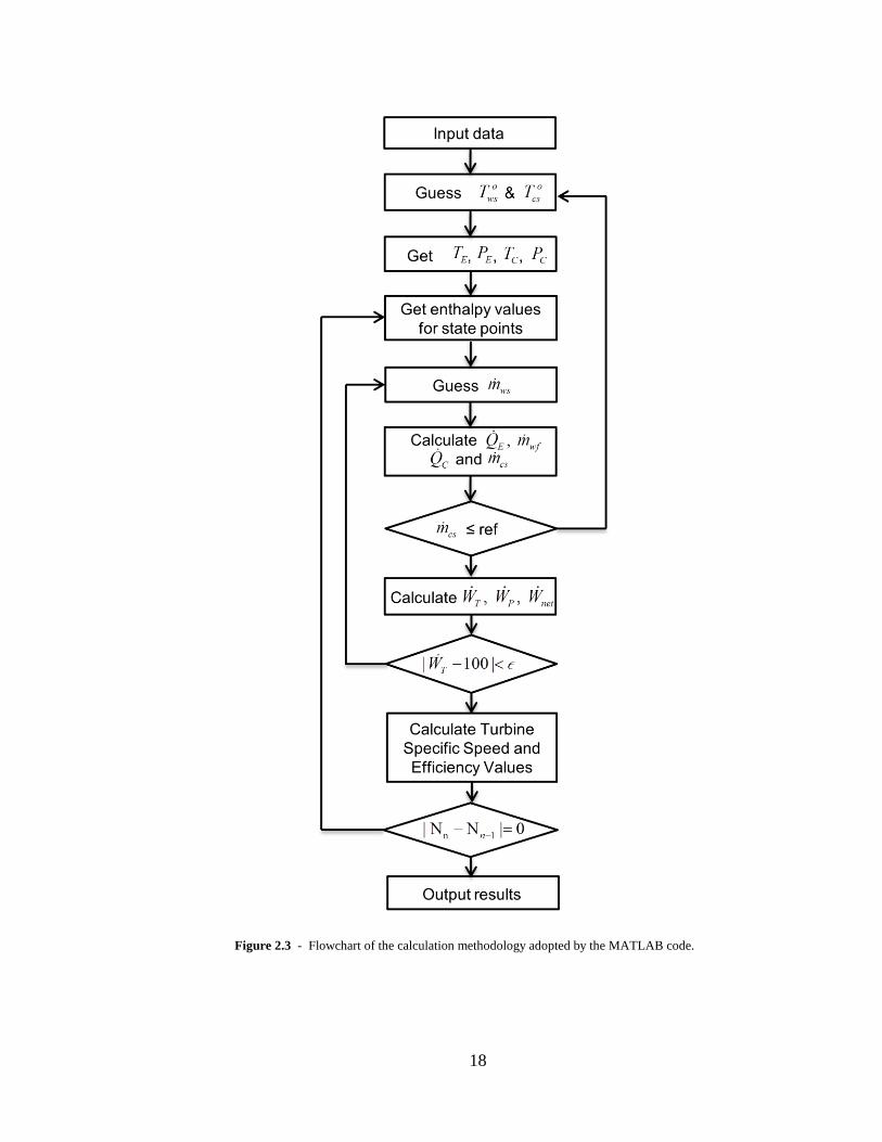
18

Figure 2.3 - Flowchart of the calculation methodology adopted by the MATLAB code.

19

2.2 Results and Discussion

Table 2.3 compiles the determined design parameters of the OTEC system that

generates a 100-kW turbine-generator power output. While our results are in overall

good agreement with previous literature about closed-cycle OTEC [14] that designed

the same scale, there are noticeable differences in some design parameters mainly due

to the use of different working fluids. Since the latent heat of vaporization for R-32

(218.59 kJ/kg-K at 290K) is almost five times smaller than that for NH3 (1064.38

kJ/kg-K at 290K), more mass flow rate is required when using R-32 as a working

fluid, resulting in more heat transfer in the evaporator and condenser. The determined

mcs / mws is 0.85, falling into the acceptable range. It should be noted that the overall

heat transfer coefficients computed in the present study agree reasonably well with

those in Ref. [14], which are experimentally obtained values from Ref. [24], indicating

that Eqs.(2.1) and (2.2) are valid correlations and can be used for different flow

conditions of seawater and working fluid at off-design operations. The estimated net

power generation is 68 kW, indicating that 32% of the turbine-generator power is

consumed by pumps. The corresponding net thermal efficiency is estimated to 1.9 %,

which is slightly lower than Ref. [14] mainly due to the bigger heat transfer rate at the

evaporator.

Figure 2.4 shows the isentropic efficiency of the turbine as a function of the

rotational speed when the turbine is designed to meet the system requirements. For the

working fluid mass flow rate of 12.3 kg/s and the enthalpy drop of 10.6 kJ/kg, the

turbine efficiency curve shows a polynomial trend to have a maximum of ~87 % at

8800 rpm.

20

Symbol Result

Seawater outlet temperature (°C)

Warm seawater T

wso 22.83

Cold seawater T

cso 8.61

Mass flow rate (kg/s)

Warm seawater mws 288.6

Cold seawater mcs 246.6

Working fluid mwf 12.3 (R-32)

Evaporator

Evaporation temperature (°C) T

E 20.83

Evaporation pressure (kPa) P

E(= P

1= P

4) 1509

Heat transfer rate (kW) QE 3660

Overall heat transfer coefficient (kW/m2 K)

U

E 3.95

Surface area (m2)

A

E 279

Condenser

Condensation temperature (°C) T

C 10.41

Condensation pressure (kPa) P

C(= P

2= P

3) 1121

Heat transfer rate (kW) QC 3561

Overall heat transfer coefficient (kW/m2 K)

U

C 3.26

Surface area (m2)

A

C 334

Power output/consumption (kW)

Turbine-generator power output WT-G

®

100.0

Working fluid pump power consumption P,wfW

(6.2)

Warm seawater pump power consumption P,wsW (8.9)

Cold seawater pump power consumption P,csW (16.9)

Net power output WN

® 68.0

Turbine isentropic efficiency (%) T 80.6

Net thermal efficiency (%) th 1.9

Table 2.3 - Design-point analysis simulation results for the closed-cycle OTEC system with 100 kW gross

power generation.

21

However, the turbine efficiency is determined to be 80.6 % at the design-point

operation, corresponding to ~12500 rpm, at which the mass flow rate of the deep

seawater meets the design requirement. As aforementioned, the mass flow rate of the

deep seawater is a more stringent design condition than the turbine efficiency for the

economic construction and operation of OTEC plants. Moreover, a turbine designed at

higher rotational speeds is more compact and guarantees a better performance when

the enthalpy drop across the turbine is demanding. For the design rotational speed of

12500 rpm; rotor tip speed and rotor tip radius of the radial inflow turbine to be used

Figure 2.4 - Turbine isentropic efficiency as a function of shaft rotational speed under design-point conditions,

i.e., wfm 12.3 kg/s and wfh 10.6 kJ/kg. The design point of the turbine operation is determined to be

approximately at 12500 rpm, yielding the turbine efficiency of 80.6 %.

22

for this particular OTEC system are determined to be 102.3 m/s and 15.6 cm,

respectively, by using Eqs.(1.18), (1.19) and (1.20).

23

CHAPTER III:

Off-Design Performance Analysis of OTEC

3.1 OTEC with Solar Thermal Collection

Since the closed-cycle OTEC system is based on the Rankine thermodynamic

cycle, its net power generation and thermal efficiency can be improved by increasing

the temperature difference between the heat source and the heat sink [15]. This study

considers two different ways to improve the performance of the OTEC system, i.e.,

preheating of the warm seawater and superheating of the working fluid using solar

energy. When the solar preheater/superheater is integrated with the base OTEC

system, the system will shift from its design point to find its new state of balance. For

the off-design point calculation, an iterative algorithm is developed to revisit the

energy balance equations at each component and to find out a converged solution.

During the off-design analysis, the geometrical parameters of the OTEC system, such

as the effective surface areas of the heat exchangers and the rotor tip radius of the

turbine, remains the same as the pre-designed values.

The net thermal efficiency for the solar preheating/superheating OTEC system is

determined by considering the additional solar energy input, i.e., E S/ ( )th NW Q Q

, where QS is the absorbed solar energy. However, since solar preheating/superheating

does not consume exhaustible energy sources, such as fossil fuels, the conventional

net thermal efficiency may underestimate the OTEC efficiency at off-design operation

conditions. Instead of simply comparing the net power generation to the total heat

24

input, more emphasis should be given to the increase of the useful net power

generation out of the total power increase when consuming additional solar energy. To

address this issue, Wang et al [9] suggested the net cycle efficiency defined as

T-GNC NW W (3.1)

which compares the net power generation of the system to the turbine-generator power

output. However, it should be noted that since the net cycle efficiency compares the

off-design performance of the system to its design-point; it should not be used to

compare between different energy conversion systems.

Since the solar collector for the OTEC system does not need a high concentration

of solar irradiation, a CPC (compound parabolic concentrator) type solar collector is

chosen as the solar thermal preheater/superheater in this study. CPC-type solar

collectors provide economical solar power concentration for low- to medium-pressure

steam systems, providing high collector efficiency in the moderate temperature range

(i.e., 80-150 °C) [30], [31]. They also can effectively collect diffuse radiation,

especially at lower concentration ratios, demonstrating satisfactory performance even

in cloudy weather [31], [32]. The overall thermal efficiency of the CPC solar collector

can be written as [33]

S 0

.Ls

r

U TF

G R

(3.2)

where Fs is the generalized heat removal factor, 0 is the optical efficiency, UL is

overall thermal loss coefficient, T is the temperature difference between the inlet

heat transfer fluid temperature and the ambient temperature, Gr is total solar

irradiation and R is the concentration ratio. Generalized Fs is a function of boiling

25

status and concentration ratio and is taken from the data available in literature [33].

Optical efficiency is assumed to be constant and taken as 80%. UL is a variable that

correlates with many factors led by temperature and is taken from measured data for a

similar CPC type solar collector [34]. Figure 3.1 shows the collector thermal

efficiency of a typical CPC solar collector as a function of / rT G (m2-K/W), when

0 is 80%, Fs varies between 0.95 and 0.90, and UL varies from 1 to 1.64 as a result of

temperature change. The solar irradiation is assumed to be 500 W/m2, which is

approximately the daytime average in Honolulu, Hawaii during the summer [35], and

the concentration ratio is set to be 3, a typical value that would provide the high

Figure 3.1 - Collector thermal efficiency of a CPC-type solar collector with a concentration

ratio of 3, oriented in the East-West direction during daytime in the summer facing South in

Honolulu, Hawaii. From the given conditions, the collector thermal efficiency is calculated to

be 65 %.

26

energy gain [36]. At the given circumstances, the resulting collector efficiency is

determined to be 65%, which is used to estimate the required collector effective area

from the following energy balance equation:

ws(wf)

S

S

[ ]

r

m hA

G

(3.3)

Here, m is the mass flow rate and h is the enthalpy change at the preheater or

superheater. The subscript “ws(wf)” indicates that the warm seawater should be

considered for preheating and the working fluid for superheating.

3.2 Solar Preheating of Seawater

As shown in Fig. 3.2, an add-on solar thermal preheater is installed next to the

evaporator side of the pre-designed OTEC system to preheat the incoming surface

seawater. The solar preheater has its own heat transfer fluid (typically

Figure 3.2 - Schematic illustration of a closed-cycle OTEC system combined

with a solar thermal energy collector to provide preheating of the surface seawater.

27

synthetic/hydrocarbon oils or water [37]) that indirectly deliver solar energy to the

seawater via the auxiliary heat exchanger. The preheated surface seawater will alter

the design operation condition of the turbine, allowing more energy extraction from

the working fluid. The off-design operation of the turbine should be fully

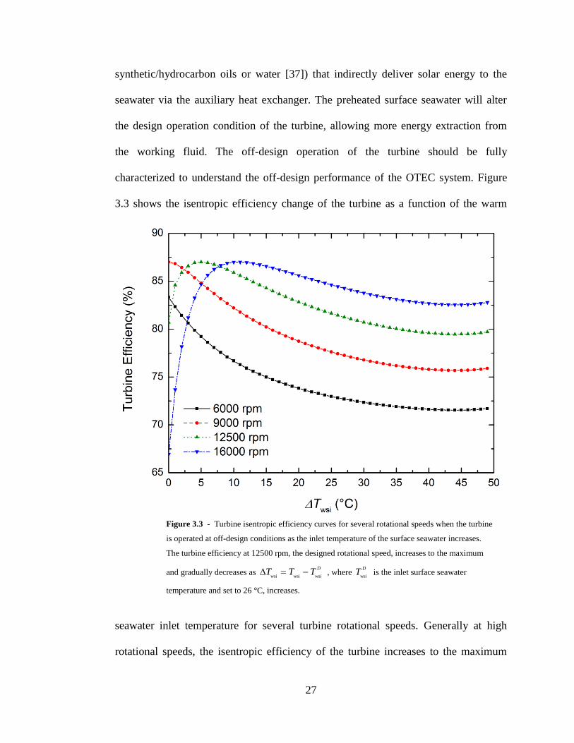
characterized to understand the off-design performance of the OTEC system. Figure

3.3 shows the isentropic efficiency change of the turbine as a function of the warm

seawater inlet temperature for several turbine rotational speeds. Generally at high

rotational speeds, the isentropic efficiency of the turbine increases to the maximum

Figure 3.3 - Turbine isentropic efficiency curves for several rotational speeds when the turbine

is operated at off-design conditions as the inlet temperature of the surface seawater increases.

The turbine efficiency at 12500 rpm, the designed rotational speed, increases to the maximum

and gradually decreases as wsi wsi wsi

DT T T , where

wsi

DT is the inlet surface seawater

temperature and set to 26 °C, increases.

28

and gradually decreases as the warm seawater inlet temperature increases. When the

turbine rotational speed is fixed at the design point, i.e., 12500 rpm, the turbine

efficiency becomes a maximum of ~87% when the preheated seawater temperature is

~31 °C. At lower rotational speeds, the overall efficiency experiences a monotonic,

gradual decrease. However, it should be noted that the preheating of the warm

seawater increases the enthalpy of the working fluid at the inlet of the turbine, which

may increase the power output despite its efficiency decrease. In order to address these

off-design characteristics of the turbine, the present study controls the mass flow rate

of the working fluid to maintain the turbine efficiency at the designed value.

Figure 3.4 shows the simulation results of the OTEC system when the ocean

water is preheated. The net power output slightly increases as the solar power

absorption at the preheater increases up to 3000 kW, then begins to substantially

increase as the solar power absorption further increases. The existence of these two

regions is mainly due to the control algorithm selected in this study. The priority in the

control algorithm is to maintain the turbine efficiency at the design point of 80.6 %.

As the inlet temperature of the surface seawater increases due to preheating, the

enthalpy drop of the working fluid across the turbine should increase and, as shown in

Eq.(1.17), the mass flow rate of the working fluid should also increase to keep ns and

the turbine efficiency at the design point. Preheating the warm seawater at its design-

point mass flow rate would put immense heat load on solar collection, demanding

massive thermal collector effective area. In order to proactively minimize this extra

load while still taking advantage of preheating and higher temperatures of the heat

source, mass flow rate of the warm seawater is controlled to provide the adequate

29

amount of heat to the working fluid at the evaporator, which is also controlled to

Figure 3.4 - Off-design simulation results of the OTEC system when preheating of

the surface seawater is implemented: (a) Change in net power generation of the

combined system and (b) change in mass flow rates of the working fluid and warm

seawater.

30

maintain the turbine efficiency at the design point. In Fig. 3.4(b), the working fluid

mass flow rate slightly increases in the low preheating range up to 3000 kW of solar

power absorption, where the surface seawater mass flow rate is drastically reduced.

This decreasing of the mass flow rate of warm seawater results in less power

consumption at the surface seawater pump, thus contributing to the slight increase of

the net power generation. In this region, as shown in Fig. 3.5(a) the net thermal

efficiency remains almost the same as the design point, suggesting that the most of the

absorbed solar energy be used to enhance the net power output.

When the solar thermal absorption becomes 3000 kW, the preheated seawater

temperature reaches the point at which the net power generation cannot increase any

more unless the working fluid is superheated. At this point, the surface seawater mass

flow rate is reduced to 48.5 kg/s, which is then fixed for further preheating to allow

the superheating of the working fluid: see Fig. 3.4(b). The control algorithm in the

second regime controls only the mass flow rate of the working fluid, leading to the

almost linear increase as the solar power absorption increases. As can be seen in Fig.

3.4(a), the net power generation drastically increases by around 25%, up to 83 kW,

mainly due to the superheating of the working fluid. However, the net thermal

efficiency drops down to ~1 %, indicating that not all the absorbed solar energy is

used in the OTEC system. However, net cycle efficiency in Fig. 3.5(a) shows an

overall improvement of the system from 71 % to 76 %, indicating that the solar energy

produces more useful net power out of the gross power generation.

31

The partial use of the solar energy for the excessive preheating is manifested by

the increase of the outlet seawater temperature at the evaporator shown in Fig. 3.5(b).

Figure 3.5 - Off-design simulation results of the OTEC system when preheating of the surface

seawater is integrated: (a) Net thermal efficiency and net cycle efficiency of the system as a

function of solar power absorption; (b) temperature difference between warm seawater and the

working fluid at evaporator inlet, i.e., wsi 1

T T , and temperature of outlet warm seawater as a

function of solar power absorption.

32

In the first region, the exiting surface seawater temperature is lower than the design

point, indicating that more thermal energy is transferred from the seawater and

converted to the power generation. However, further preheating drastically increases

the exit temperature of the seawater, which reaches up to ~50 °C when the solar power

absorption becomes 8500 kW. This inefficient use of absorbed solar energy is because

of the limited surface area of the evaporator and condenser, which are originally

optimized at the 100-kW turbine-generator power capacity. Moreover, unless this hot

seawater is used somewhere else, returning it back to the ocean might cause adverse

environmental and ecological impacts. The hot seawater could be used to reheat the

working fluid by installing a second turbine, which can extract more work out of the

working fluid vapor before it enters the condenser. However, current research focuses

on the effect of solar preheating on an existing OTEC system and thus did not consider

further modification of the system besides the installation of the solar preheater.

Figure 3.5(b) also shows the temperature difference between the incoming seawater

and the exiting working fluid vapor, i.e., wsi 1T T at the evaporator. In the first region,

this temperature difference keeps increasing because the control algorithm does not

allow the superheating of the working fluid: thus T1 in this range is the same as the

evaporation temperature of the working fluid. However, in the second regime, the

superheating of the working fluid reduces wsi 1T T below the value of the design-point

pinch point temperature difference. Thus the practical limit of the seawater preheating

occurs at the evaporator inlet of the warm seawater unless the evaporator is replaced

with a bigger one.

33

3.3 Solar Superheating of Working Fluid

Evidently from the simulation results, preheating the ocean water requires huge

amount of solar energy due to massive flow rate and high specific heat capacity of

water, demanding a large effective area of the solar collector despite the aggressive

reduction of the mass flow rate. On the other hand, difluoromethane (R-32) has a

significantly lower specific heat, and its mass flow rate is much smaller than that of

the surface seawater. Therefore, superheating the working fluid by solar heating

should improve the OTEC cycle with much less solar energy required. As shown in

Fig. 3.6, an add-on solar thermal converter is attached between the evaporator and the

turbine of the pre-designed OTEC system to superheat the working fluid. The solar

superheater, same as in the preheating case, has its own heat transfer fluid and

Figure 3.6 - Schematic illustration of a closed-cycle OTEC

system combined with a solar thermal energy collector to

provide superheating of the working fluid.

34

provides the heating to the working fluid via the auxiliary heat exchanger.

Simulation results for superheating, as can be seen in Fig. 3.7, reveals that

Figure 3.7 - Off-design simulation results of the OTEC system when superheating of the

working fluid is considered: (a) Change in net power generation of the combined system

with solar power absorption and (b) the net thermal efficiency and net cycle efficiency of

the system as a function of solar power absorption.

35

thermal efficiency of the OTEC cycle is improved from 1.9 % to 3 % as the solar

energy is more absorbed for superheating. This efficiency increase directly results in

more net power generation from 68 kW to 85 kW, enhanced by 25% from design-

point. Net cycle efficiency of the system also increases from 71 % to 76 %, which is in

a similar trend to the preheating case. The improvement of both efficiencies

demonstrates that the absorbed solar energy is effectively utilized to generate more

useful net power than the design-point. The net thermal efficiency of the combined

system could be theoretically further increased until the critical temperature of R-32 is

reached at around 78 °C. However, this extreme superheating will cause the working

fluid vapor to remain superheated at the exit of the turbine, undesirably requiring more

mass flow rate of the deep seawater at the condenser. The present study simulates only

the sub-critical superheating case, where the vapor quality of the working fluid at the

exit of the turbine remains around unity.

Figure 3.8 shows the mass flow rate and the turbine inlet temperature of the

working fluid as a function of the solar power absorption. As the solar power

absorption increases, the system needs more working fluid mass flow rate to

effectively convert the absorbed solar energy to the turbine-generator power. The

increase of the solar power absorption also leads to more superheating of the working

fluid and, correspondingly, more enthalpy drop in the turbine. As discussed in the

preheating case, the mass flow rate of the working fluid and the enthalpy drop are

correlated in Eq.(1.17). Thus the mass flow rate of R-32 should be controlled to

operate the turbine at the design-point while fully utilizing the solar power absorption.

36

3.4 Results and Discussion

Figure 3.9 shows the required effective area of the solar collector when used for

preheating the surface seawater. When plotted as a function of the net power output,

the collector effective area has a sudden jump to ~2000 m2 to enhance the net power

from 68 kW to 70 kW, or only ~3% increase from the design point. A larger collector

effective area should be installed to take considerable advantage of the solar

preheating: for example, nearly 6000 m2 of the collector area is needed to increase the

Figure 3.8 - Turbine inlet temperature of the superheated working fluid vapor and its mass

flow rate as a function of solar power absorption, as results of the off-design simulation when

superheating of the working fluid is implemented.

37

net power of the system by ~20%. The collector area could be significantly reduced by

improving the design of the collector or using a different heat transfer fluid that has a

higher solar absorption coefficient.

Potential adverse environmental effects due to increased seawater temperature at

the surface of the ocean as a result of the preheating method could be addressed by

simply making use of this excess heat. This could very well be accomplished by

adding a second stage turbine and implementing reheating in the OTEC cycle.

Secondary applications that are popular with OTEC are also on the table such as

desalination to produce potable water or to be used in irrigation.

Figure 3.9 - Required collector effective area of a solar preheater as a function of net

power generation of the system, according to the off-design simulation results of the OTEC

system when preheating of the surface seawater is implemented.

38

Figure 3.10 shows the required collector effective area as a function of net power

generation for the superheating case. When compared to the preheating case, much

less collector effective area is required for the superheater to obtain the same amount

of net power enhancement. For example, around 1100 m2 of collector effective area is

needed to obtain 20% more net power in the superheating case, which needs only

~18% of the collector area when the preheating is used. This result strongly suggests

that the solar superheater may be more beneficial in improving the OTEC system

although it requires more care to prevent leakage of the working fluid into the

environment during long-term operation [15].

Figure 3.10 - Required collector effective area of a solar superheater as a function of net

power generation, in accordance with the off-design simulation results of the OTEC system

when superheating of the working fluid is considered.

39

CHAPTER IV:

Conclusion

4.1 Summary of Results and Findings

This thesis presented research about the thermodynamic effects of solar thermal

preheating/superheating on the performance of a closed-cycle OTEC system. For this

purpose, a closed-cycle OTEC system capable of generating 100 kW gross power was

designed numerically. This system constituted the base OTEC system to be improved

thermodynamically. Designed system using difluoromethane (R-32) as its working

fluid was able to produce 68 kW of net power with net thermal efficiency of 1.9 % and

net cycle efficiency of ~70 %. Next, off-design performance analysis was conducted

with the addition of a CPC type solar thermal collector integrated with the predesigned

OTEC system, acting firstly as a preheater of the surface seawater and then as a

superheater of the working fluid.

Simulation results demonstrate an improvement of the net power generation by

up to 20-25% from the design-point for both the preheating and superheating cases.

However, superheating of the working fluid requires up to 4 times less solar collector

effective area when compared to preheating of the ocean water. Additionally, it has

virtually no adverse environmental effects on the ocean and marine life, whereas

preheating results in increased surface seawater temperature unless this extra heat is

used or dispersed elsewhere. Superheating method also increased the thermal

efficiency of the system from 1.9 % to ~3%, about 60% improvement, suggesting that

it might be a better approach in improving an OTEC system.

40

4.2 Recommendations for Further Research

The collector area required for preheating/superheating in OTEC could be

significantly reduced by improving the design of the collector or using a different heat

transfer fluid that has a higher solar absorption coefficient. Previous studies revealed

that mixing nanoparticles into the fluid can enhance the light absorptance to almost

100% above a certain nanoparticle concentration [38], [39], [40], [41]. This

enhancement of the light absorptance directly affects the solar collector efficiency,

e.g., ~10% increase of efficiency when aluminum nanoparticles are suspended in

water [39]. Increasing collector efficiency would in return increase overall thermal

efficiency of the combined system and also reduce the production costs. To that end,

looking into different shapes and configurations of plasmonic nanoparticles and

considering a solar thermal collection system that has a strong light absorption over a

broad spectrum from the visible to the near-infrared range would be worthwhile.

41

APPENDICES

Appendix A: REFPROP Matlab Code [25]

%%%%%%%%%%%%%%%%%%%%%%%%%%%%%%%%%%%%%%%%%%%%%%%%%%%%%%%%%%%%%%%%%%%%%%%%%%% % refpropm Thermophysical properties of pure substances and mixtures. % Calling sequence for pure substances: % result=refpropm(prop_req, spec1, value1, spec2, value2, substance1) % % Calling predefined mixtures: % result=refpropm(prop_req, spec1, value1, spec2, value2, mixture1) % % Calling user defined mixtures: % result=refpropm(prop_req, spec1, value1, spec2, value2, % substance1, substance2, ..., x) % % where % prop_req character string showing the requested properties % Each property is represented by one character: % 0 Refprop DLL version number % A Speed of sound [m/s] % B Volumetric expansivity (beta) [1/K] % C Cp [J/(kg K)] % D Density [kg/m^3] % F Fugacity [kPa] (returned as an array) % G Gross heating value [J/kg] % H Enthalpy [J/kg] % I Surface tension [N/m] % J Isenthalpic Joule-Thompson coeff [K/kPa] % K Ratio of specific heats (Cp/Cv) [-] % L Thermal conductivity [W/(m K)] % M Molar mass [g/mol] % N Net heating value [J/kg] % O Cv [J/(kg K)] % P Pressure [kPa] % Q Quality (vapor fraction) (kg/kg) % S Entropy [J/(kg K)] % T Temperature [K] % U Internal energy [J/kg] % V Dynamic viscosity [Pa*s] % X Liquid phase & gas phase comp.(mass frac.) % Z Compressibility factor % $ Kinematic viscosity [cm^2/s] % % Thermal diffusivity [cm^2/s] % ^ Prandtl number [-] % + Liquid density of equilibrium phase % - Vapor density of equilibrium phase % % E dP/dT (along the saturation line) [kPa/K] % # dP/dT (constant rho) [kPa/K] % R d(rho)/dP (constant T) [kg/m^3/kPa]

42

% W d(rho)/dT (constant p) [kg/(m^3 K)] % ! dH/d(rho) (constant T) [(J/kg)/(kg/m^3)] % & dH/d(rho) (constant P) [(J/kg)/(kg/m^3)] % ( dH/dT (constant P) [J/(kg K)] % @ dH/dT (constant rho) [J/(kg K)] % * dH/dP (constant T) [J/(kg kPa)] % % spec1 first input character: T, P, H, D, C, R, or M % T, P, H, D: see above % C: properties at the critical point % R: properties at the triple point % M: properties at Tmax and Pmax % (Note: if a fluid's lower limit is higher % than the triple point, the lower limit will % be returned) % % value1 first input value % % spec2 second input character: P, D, H, S, U or Q % % value2 second input value % % substance1 file name of the pure fluid (or the first % component of the mixture) % % mixture1 file name of the predefined fluid mixture % with the extension ".mix" included % % substance2,substance3,...substanceN % name of the other substances in the % mixture. Up to 20 substances can be handled. % Valid substance names are equal to the file names % in the C:\Program Files\REFPROP\fluids\' directory. % % x vector with mass fractions of the substances % in the mixture. % % Examples: % 1) P = refpropm('P','T',373.15,'Q',0,'water') gives % Vapor pressure of water at 373.15 K in [kPa] % % 2) [S Cp] = refpropm('SC','T',373.15,'Q',1,'water') gives % Entropy and Cp of saturated steam at 373.15 K % % 3) D = refpropm('D','T',323.15,'P',1e2,'water','ammonia',[0.9 0.1]) % Density of a 10% ammonia/water solution at 100 kPa and 323.15 K. % % 4) [x y] = refpropm('X','P',5e2,'Q',0.4,'R134a','R32',[0.8, 0.2]) % Temperature as well as gas and liquid compositions for a mixture % of two refrigerants at a certain pressure and quality. % Note that, when 'X' is requested, two variables must be sent, the % first contains the liquid phase composition and the second % the vapor phase composition. % % 5) T=refpropm('T','C',0,' ',0,'water')

43

% Critical temperature % % 6) T=refpropm('T','M',0,' ',0,'r410a.mix') % Maximum temperature that can be used to call properties. % Shows how to call a predefined mixture. % %%%%%%%%%%%%%%%%%%%%%%%%%%%%%%%%%%%%%%%%%%%%%%%%%%%%%%%%%%%%%%%%%%%%%%%%%%% % % Originally based on the file refpropm.f90. % % Credits: % Paul M. Brown, Ramgen Power Systems, Inc. 2004-05-17 % Modified input parameters to make 'HS' calls % Interface now handles 'HP', 'HD' and 'HT' as well % Fixed P_rp calculation for spec2='P' case (moved calc earlier) % Added property requests for Cv (O), gamma (K) and speed of sound (A) % % Johannes Lux, German Aerospace Center 2006-03-30 % Modified input pressure unit back to [Pa] % Interface now works with Matlab R2006a (.mexw32 file format instead of .dll file format) % Continuation lines modified to be compatible with Compaq Visual Fortran 9.0 % No wrong results return with the first call anymore % Changed name to "refpropm.f90" to avoid name conflicts with Matlab % Function call is for example: % refpropm(prop_req, spec1, value1, spec2, value2, substance1) % Fluid files are located in C:\Program Files\REFPROP\fluids\ % new version 7.2 beta, compiled using Matlab R2006a (2006-10-08) % new version 7.2 beta (2006-10-24), compiled using Matlab R2006a % new version 8.0 beta (2007-01-18), compiled using Matlab R2006b % Modified input pressure unit back to [kPa] (2007-02-22) % % Chris Muzny, NIST % made changes for 2009a compatibility and 64-bit execution % % Eric Lemmon, NIST % allow .ppf files to be loaded % allow .mix files to be loaded % add molar mass, heating values % add HQ input, critical parameters % add fugacity, beta, dH/d(rho) % % Keith Wait, Ph.D, GE Appliances 2011-07-01 % [email protected] % Translated to Matlab native code, known to work against Matlab % 2010b. Fortran compiler no longer necessary to add new properties, % make other modifications. % Added outputs B, E, F, J, and R. % HQ input regressed. %%%%%%%%%%%%%%%%%%%%%%%%%%%%%%%%%%%%%%%%%%%%%%%%%%%%%%%%%%%%%%%%%%%%%%%%%%% function varargout = refpropm( varargin ) ierr = 0;

44

q = 999; e = 0; h = 0; s = 0; cv = 0; cp = 0; w = 0; hjt = 0; phaseFlag = 0; archstr = computer('arch'); libName = 'refprop'; dllName = 'REFPROP.dll'; prototype = @rp_proto; % Input Sanity Checking nc_base = 5; if (nargin == 6) numComponents = 1; elseif (nargin < 6) error('Too few input arguments, should be 6 or more'); elseif (nargin > 26) error('Too many input arguments'); else numComponents = nargin - nc_base - 1; end fluidType = []; for i = 1:numComponents fluidType = [fluidType char(varargin(5+i))]; end % Load DLL RefpropLoadedState = getappdata(0, 'RefpropLoadedState'); if ~libisloaded(libName) switch computer case {'GLNXA64', 'GLNX86', 'MACI', 'MACI64', 'SOL64'} BasePath = '/usr/local/REFPROP/'; FluidDir = 'FLUIDS/'; otherwise BasePath = 'C:\Program Files\REFPROP\'; FluidDir = 'fluids\'; if ~exist(BasePath,'dir') BasePath = 'C:\Program Files (x86)\REFPROP\'; end if archstr == 'win64' %If you are using a 64 bit version of MatLab, please contact Eric Lemmon for the DLL listed below. ([email protected]) dllName = 'REFPRP64.dll'; prototype = @() rp_proto64(BasePath); end end

45

% v=char(calllib('REFPROP','RPVersion',zeros(255,1))'); % Useful for debugging... RefpropLoadedState = struct('FluidType', 'none', 'BasePath', BasePath, 'FluidDir', FluidDir, 'nComp', 0, 'mixFlag', 0, 'z_mix', 0); setappdata(0, 'RefpropLoadedState', RefpropLoadedState); % the following returns 0 if refprop.dll does not exist, 1 if refprop.dll is a variable name in the workspace, 2 if C:\Program Files (x86)\REFPROP\refprop.dll exist, and 3 if refprop.dll exist but is a .dll file in the MATLAB path if ~ismember(exist(strcat(BasePath, dllName),'file'),[2 3]) dllName = lower(dllName); end if ~ismember(exist(strcat(BasePath, dllName),'file'),[2 3]) error(strcat(dllName,' could not be found. Please edit the refpropm.m file and add your path to the lines above this error message.')); end [notfound,warnings]=loadlibrary(strcat(BasePath,dllName),prototype,'alias',libName); end % Prepare REFPROP if ~strcmpi(fluidType, RefpropLoadedState.FluidType) fluidFile = ''; RefpropLoadedState.FluidType = ''; RefpropLoadedState.mixFlag = 0; setappdata(0, 'RefpropLoadedState', RefpropLoadedState); if strfind(lower(fluidType), '.mix') ~= 0 RefpropLoadedState.mixFlag = 1; fluidName = fluidType; fluidFile = strcat(RefpropLoadedState.BasePath, 'mixtures\',fluidName); hmxnme = [unicode2native(fluidFile) 32*ones(1,255-length(fluidFile))]'; mixFile = strcat(RefpropLoadedState.BasePath, ... RefpropLoadedState.FluidDir, 'hmx.bnc'); hmix = [unicode2native(mixFile) 32*ones(1,255-length(mixFile))]'; href = unicode2native('DEF')'; [hmxnme hmix href nc path z ierr errTxt] = calllib(libName,'SETMIXdll',hmxnme,hmix,href,0,32*ones(10000,1),zeros(1,20),0,32*ones(255,1),255,255,3,10e3,255); else for i = 1:numComponents fluidName=char(varargin(i+5)); if isempty(strfind(lower(fluidName),'.fld')) if isempty(strfind(lower(fluidName),'.ppf')) fluidName = strcat(fluidName,'.fld'); end end fluidFile = strcat(fluidFile, RefpropLoadedState.BasePath, ... RefpropLoadedState.FluidDir,fluidName,'|');

46

end path = [unicode2native(fluidFile) 32*ones(1,10e3-length(fluidFile))]'; mixFile = strcat(RefpropLoadedState.BasePath, ... RefpropLoadedState.FluidDir, 'hmx.bnc'); hmix = [unicode2native(mixFile) 32*ones(1,255-length(mixFile))]'; href = unicode2native('DEF')'; [nc path hmix href ierr errTxt] = calllib(libName,'SETUPdll',numComponents,path,hmix,href,0,32*ones(255,1),10000,255,3,255); z = 1; end if (ierr > 0) error(char(errTxt')); end %Use the call to PREOSdll to change the equation of state to Peng Robinson for all calculations. %To revert back to the normal REFPROP EOS and models, call it again with an input of 0. % [dummy] = calllib(libName,'PREOSdll',2); %To enable better and faster calculations of saturation states, call the %subroutine SATSPLN. However, this routine takes several seconds, and %should be disabled if changing the fluids regularly. %This call only works if a *.mix file is sent. %You may also need to uncomment the declaration of SATSPLN in the rp_proto.m file. % [dummyx ierr errTxt] = calllib(libName,'SATSPLNdll', z, 0, 32*ones(255,1), 255); % Use the following line to calculate enthalpies and entropies on a reference state % based on the currently defined mixture, or to change to some other reference state. % The routine does not have to be called, but doing so will cause calculations % to be the same as those produced from the graphical interface for mixtures. % [href dummy dummy dummy dummy dummy ierr2 errTxt] = calllib(libName, 'SETREFdll', href, 2, z, 0, 0, 0, 0, 0, 32*ones(255,1), 3, 255); RefpropLoadedState.z_mix = z; RefpropLoadedState.nComp = nc; RefpropLoadedState.FluidType = lower(fluidType); setappdata(0, 'RefpropLoadedState', RefpropLoadedState); end numComponents = RefpropLoadedState.nComp; % Extract Inputs from Varargin propReq = lower(char(varargin(1))); propTyp1 = lower(char(varargin(2))); propTyp2 = lower(char(varargin(4))); propVal1 = cell2mat(varargin(3));

47

propVal2 = cell2mat(varargin(5)); herr = 32*ones(255,1); if length(propReq)==2 if propReq(2)=='>' propReq = propReq(1); phaseFlag=1; elseif propReq(2)=='<' propReq = propReq(1); phaseFlag=2; end end % Calculate Molar Mass if numComponents == 1 z = 1; elseif RefpropLoadedState.mixFlag == 0 z_kg = cell2mat(varargin(nargin)); if length(z_kg) ~= numComponents error('Mass fraction must be given for all components'); elseif abs(sum(z_kg)-1) > 1e-12 error('Mass fractions must sum to 1'); end [dummyx z molw] = calllib(libName,'XMOLEdll',z_kg,zeros(1,numComponents),0); elseif RefpropLoadedState.mixFlag == 1 z = RefpropLoadedState.z_mix; end [dummyx molw] = calllib(libName,'WMOLdll',z,0); molw = molw*1e-3; % Sanity Check Provided Property Types if propTyp1 == propTyp2 error('Provided values are the same type'); end varargout = cell(size(propReq)); switch propTyp1 case 'p' P_rp = propVal1; case 't' T = propVal1; case 'd' D_rp = propVal1 * 1e-3 / molw; case 'h' h = propVal1 * molw; case 'c' if numComponents == 1 [dummy wm ttp tnbp T P_rp D_rp zc acf dip rgas] = calllib(libName,'INFOdll', 1, 0, 0, 0, 0, 0, 0, 0, 0, 0, 0); else [dummy T P_rp D_rp ierr errTxt] = calllib(libName,'CRITPdll', z, 0, 0, 0, 0, herr, 255);

48

end [dummy dummy dummy pp e h s cv cp w hjt] = calllib(libName,'THERMdll', T, D_rp, z, 0, 0, 0, 0, 0, 0, 0, 0); case 'r' if numComponents == 1 heos = unicode2native('EOS')'; [heos dummy dummy dummy dummy T tmax Dmax pmax ierr errTxt] = calllib(libName,'LIMITXdll', heos, 300, 0, 0, z, 0, 0, 0, 0, 0, herr, 3, 255); if strncmp(RefpropLoadedState.FluidType,'water',5) [dummy wm T tnbp Tc P_rp D_rp zc acf dip rgas] = calllib(libName,'INFOdll', 1, 0, 0, 0, 0, 0, 0, 0, 0, 0, 0); end if propReq=='t' varargout(1) = {T}; %Exit early if only T required, not all fluids work at Ttrp. return end [dummy dummy dummy dummy P_rp D_rp Dl Dv x y e h s cv cp w ierr errTxt] = calllib(libName,'TQFLSHdll', T, 0, z, 2, 0, 0, 0, 0, zeros(1,numComponents), zeros(1,numComponents), 0, 0, 0, 0, 0, 0, 0, herr, 255); % [dummy dummy dummy P_rp Dl Dv x y ierr errTxt] = calllib(libName, 'SATTdll', T, z, 1, 0, 0, 0, zeros(1,numComponents), zeros(1,numComponents), 0, herr, 255); else error('Triple point not known for mixtures'); end case 'm' heos = unicode2native('EOS')'; [heos dummy dummy dummy dummy tmin T Dmax P_rp ierr errTxt] = calllib(libName,'LIMITXdll', heos, 300, 0, 0, z, 0, 0, 0, 0, 0, herr, 3, 255); [dummy dummy dummy D_rp Dl Dv x y q e h s cv cp w ierr errTxt] = calllib(libName,'TPFLSHdll', T, P_rp, z, 0, 0, 0, zeros(1,numComponents), zeros(1,numComponents), 0, 0, 0, 0, 0, 0, 0, 0, herr, 255); case '0' [dummy dummy dummy dummy ierr errTxt] = calllib(libName,'SETUPdll',-1,10000*ones(255,1),255*ones(255,1),3*ones(255,1),0,32*ones(255,1),10000,255,3,255); varargout(1)={double(ierr)/10000}; return otherwise error('Provided value 1 is not P, T, H, D, C, R, or M'); end switch propTyp2 case 'p' P_rp = propVal2; case 'd' D_rp = propVal2 * 1e-3 / molw; case 'h' h = propVal2 * molw; case 's' s = propVal2 * molw;

49

case 'u' e = propVal2 * molw; case 'q' q = propVal2; otherwise if (propTyp1 ~= 'c' && propTyp1 ~= 'r' && propTyp1 ~= 'm' ) error('Provided value 2 is not P, H, S, U, Q, or D'); end propTyp2 = ' '; end % Call Appropriate REFPROP Flash Function According to Provided Property Types if ((propTyp1 == 'p') && (propTyp2 == 'd')) || ((propTyp2 == 'p') && (propTyp1 == 'd')) [dummy dummyx dummy T Dl Dv x y q e h s cv cp w ierr errTxt] = calllib(libName,'PDFLSHdll',P_rp, D_rp, z, 0, 0, 0, zeros(1,numComponents), zeros(1,numComponents), 0, 0, 0, 0, 0, 0, 0, 0, herr, 255); elseif ((propTyp1 == 'p') && (propTyp2 == 'h')) || ((propTyp2 == 'p') && (propTyp1 == 'h')) if phaseFlag==0 [dummy dummy dummyx T D_rp Dl Dv x y q e s cv cp w ierr errTxt] = calllib(libName,'PHFLSHdll',P_rp, h, z, 0, 0, 0, 0, zeros(1,numComponents), zeros(1,numComponents), 0, 0, 0, 0, 0, 0, 0, herr, 255); else [dummy dummy dummyx dummy T D_rp ierr errTxt] = calllib(libName,'PHFL1dll',P_rp, h, z, phaseFlag, 0, 0, 0, herr, 255); [dummy dummy dummyx P_rp e h s cv cp w hjt] = calllib(libName,'THERMdll', T, D_rp, z, 0, 0, 0, 0, 0, 0, 0, 0); end elseif ((propTyp1 == 'p') && (propTyp2 == 't')) || ((propTyp2 == 'p') && (propTyp1 == 't')) if phaseFlag==0 [dummy dummy dummyx D_rp Dl Dv x y q e h s cv cp w ierr errTxt] = calllib(libName,'TPFLSHdll', T, P_rp, z, 0, 0, 0, zeros(1,numComponents), zeros(1,numComponents), 0, 0, 0, 0, 0, 0, 0, 0, herr, 255); else [dummy dummy dummyx dummy dummy D_rp ierr errTxt] = calllib(libName,'TPRHOdll', T, P_rp, z, phaseFlag, 0, 0, 0, herr, 255); [dummy dummy dummyx P_rp e h s cv cp w hjt] = calllib(libName,'THERMdll', T, D_rp, z, 0, 0, 0, 0, 0, 0, 0, 0); end elseif ((propTyp1 == 'h') && (propTyp2 == 'd')) || ((propTyp2 == 'h') && (propTyp1 == 'd')) [dummy dummy dummyx T P_rp Dl Dv x y q e s cv cp w ierr errTxt] = calllib(libName,'DHFLSHdll', D_rp, h, z, 0, 0, 0, 0, zeros(1,numComponents), zeros(1,numComponents), 0, 0, 0, 0, 0, 0, 0, herr, 255); elseif ((propTyp1 == 't') && (propTyp2 == 'd')) || ((propTyp2 == 't') && (propTyp1 == 'd')) [dummy dummy dummyx P_rp Dl Dv x y q e h s cv cp w ierr errTxt] = calllib(libName,'TDFLSHdll', T, D_rp, z, 0, 0, 0, zeros(1,numComponents), zeros(1,numComponents), 0, 0, 0, 0, 0, 0, 0, 0, herr, 255); elseif ((propTyp1 == 't') && (propTyp2 == 'h')) || ((propTyp2 == 't') && (propTyp1 == 'h'))

50

[dummy dummy dummyx dummy P_rp D_rp Dl Dv x y q e s cv cp w ierr errTxt] = calllib(libName,'THFLSHdll', T, h, z, 1, 0, 0, 0, 0, zeros(1,numComponents), zeros(1,numComponents), 0, 0, 0, 0, 0, 0, 0, herr, 255); else switch propTyp2 case 's' switch propTyp1 case 't' [dummy dummy dummyx dummy P_rp D_rp Dl Dv x y q e h cv cp w ierr errTxt] = calllib(libName,'TSFLSHdll', T, s, z, 1, 0, 0, 0, 0, zeros(1,numComponents), zeros(1,numComponents), 0, 0, 0, 0, 0, 0, 0, herr, 255); case 'p' [dummy dummy dummyx T D_rp Dl Dv x y q e h cv cp w ierr errTxt] = calllib(libName,'PSFLSHdll', P_rp, s, z, 0, 0, 0, 0, zeros(1,numComponents), zeros(1,numComponents), 0, 0, 0, 0, 0, 0, 0, herr, 255); case 'h' [dummy dummy dummyx T P_rp D_rp Dl Dv x y q e cv cp w ierr errTxt] = calllib(libName,'HSFLSHdll', h, s, z, 0, 0, 0, 0, 0, zeros(1,numComponents), zeros(1,numComponents), 0, 0, 0, 0, 0, 0, herr, 255); case 'd' [dummy dummy dummyx T P_rp Dl Dv x y q e h cv cp w ierr errTxt] = calllib(libName,'DSFLSHdll', D_rp, s, z, 0, 0, 0, 0, zeros(1,numComponents), zeros(1,numComponents), 0, 0, 0, 0, 0, 0, 0, herr, 255); end case 'u' switch propTyp1 case 't' [dummy dummy dummyx dummy P_rp D_rp Dl Dv x y q h s cv cp w ierr errTxt] = calllib(libName,'TEFLSHdll', T, e, z, 1, 0, 0, 0, 0, zeros(1,numComponents), zeros(1,numComponents), 0, 0, 0, 0, 0, 0, 0, herr, 255); case 'p' [dummy dummy dummyx T D_rp Dl Dv x y q h s cv cp w ierr errTxt] = calllib(libName,'PEFLSHdll', P_rp, e, z, 0, 0, 0, 0, zeros(1,numComponents), zeros(1,numComponents), 0, 0, 0, 0, 0, 0, 0, herr, 255); case 'd' [dummy dummy dummyx T P_rp Dl Dv x y q h s cv cp w ierr errTxt] = calllib(libName,'DEFLSHdll', D_rp, e, z, 0, 0, 0, 0, zeros(1,numComponents), zeros(1,numComponents), 0, 0, 0, 0, 0, 0, 0, herr, 255); otherwise error('HU not a supported combination'); end case 'q' switch propTyp1 case 't' [dummy dummy dummyx dummy P_rp D_rp Dl Dv x y e h s cv cp w ierr errTxt] = calllib(libName,'TQFLSHdll', T, q, z, 2, 0, 0, 0, 0,

51

zeros(1,numComponents), zeros(1,numComponents), 0, 0, 0, 0, 0, 0, 0, herr, 255); case 'p' [dummy dummy dummyx dummy T D_rp Dl Dv x y e h s cv cp w ierr errTxt] = calllib(libName,'PQFLSHdll', P_rp, q, z, 2, 0, 0, 0, 0, zeros(1,numComponents), zeros(1,numComponents), 0, 0, 0, 0, 0, 0, 0, herr, 255); % case 'd' % [dummy dummy dummyx dummy T P_rp Dl Dv x y ierr errTxt] = calllib(libName,'DQFL2dll', D_rp, q, z, 1, 0, 0, 0, 0, zeros(1,numComponents), zeros(1,numComponents), 0, herr, 255); otherwise error('HQ or DQ are not supported combinations'); end end end if (ierr > 0) error(char(errTxt')); end if ~isempty(strfind(propReq,'g')) || ~isempty(strfind(propReq,'n')) if q>0 && q<1 error('Heating value routines not valid for 2-phase states') end [dummy dummy dummyx hg hn ierr errTxt] = calllib(libName,'HEATdll',T,D_rp,z,0,0,0,herr,255); if (ierr ~= 0) error(char(errTxt')); end end if ~isempty(strfind(propReq,'v')) || ~isempty(strfind(propReq,'l')) || ~isempty(strfind(propReq,'$')) || ~isempty(strfind(propReq,'%')) || ~isempty(strfind(propReq,'^')) if q>0 && q<1 error('Transport routines not valid for 2-phase states') end [dummy dummy dummyx eta tcx ierr errTxt] = calllib(libName,'TRNPRPdll',T,D_rp,z,0,0,0,herr,255); if (ierr ~= 0) error(char(errTxt')); end end % Construct Return Vector % To add more property choices, just add a new case to this structure and % follow the examples below. for i = 1:length(propReq) switch propReq(i) case 't' varargout(i) = {T}; case 'p' varargout(i) = {P_rp}; case 'h'

52

varargout(i) = {h/molw}; case 's' varargout(i) = {s/molw}; case 'u' varargout(i) = {e/molw}; case 'd' varargout(i) = {D_rp*1e3*molw}; case 'z' varargout(i) = {P_rp/D_rp/T/8.314472e0}; case 'm' varargout(i) = {molw*1e3}; case 'g' varargout(i) = {hg/molw}; case 'n' varargout(i) = {hn/molw}; case '+' [dummy x_kg xmolw] = calllib(libName,'XMASSdll',x,zeros(1,numComponents),0); varargout(i) = {Dl*xmolw}; case '-' [dummy y_kg ymolw] = calllib(libName,'XMASSdll',y,zeros(1,numComponents),0); varargout(i) = {Dv*ymolw}; case 'q' if ((q <= 0) || (q >= 1)) varargout(i) = {q}; else [dummy wmol] = calllib(libName,'WMOLdll',y,0); varargout(i) = {q*wmol*1e-3/molw}; end case 'x' [dummyx x_kg dummy] = calllib(libName,'XMASSdll',x,zeros(1,numComponents),0); [dummyx y_kg dummy] = calllib(libName,'XMASSdll',y,zeros(1,numComponents),0); % varargout(i) = {[x_kg ;y_kg]}; if length(propReq)>1 error('Only one input is allowed when using property input X since two outputs are returned (liquid and vapor compositions).'); end varargout(i) = {x_kg'}; varargout(i+1) = {y_kg'}; case 'f' if ((q < 0) || (q > 1)) [dummy dummy dummyx f] = calllib(libName,'FGCTYdll',T,D_rp,z,zeros(1,numComponents)); else %Liquid and vapor fugacties are identical, use liquid phase here [dummy dummy dummyx f] = calllib(libName,'FGCTYdll',T,Dl,x,zeros(1,numComponents)); end varargout(i) = {f'}; case 'i' if ((q >= 0) && (q <= 1))

53

[dummy dummy dummy dummy dummy sigma ierr errTxt] = calllib(libName,'SURTENdll',T,Dl,Dv,x,y,0,0,herr,255); if (ierr ~= 0) error(char(errTxt')); end varargout(i) = {sigma}; else error('Surface tension can only be calculated for saturated conditions.'); end case 'e' if numComponents > 1 error('dP/dT (sat) not supported for mixtures'); end [dummy dummy dummyx Psat Dsat Csat dpdtSat ierr errTxt] = calllib(libName,'DPTSATKdll',1,T,1,0,0,0,0,0,herr,255); varargout(i) = {dpdtSat}; otherwise if (q>0 && q<1) error('Property not available for 2-phase states.'); else switch propReq(i) case 'c' varargout(i) = {cp/molw}; case 'o' varargout(i) = {cv/molw}; case 'k' varargout(i) = {cp/cv}; case 'a' varargout(i) = {w}; case 'v' varargout(i) = {eta*1e-6}; case 'l' varargout(i) = {tcx}; case 'b' [dummy dummy dummyx P_rp e h s cv cp w zz hjt A G xkappa beta dPdrho d2PdD2 dPT drhodT drhodP d2PT2 d2PdTD spare1 spare2] = calllib(libName,'THERM2dll',T,D_rp,z,0,0,0,0,0,0,0,0,0,0,0,0,0,0,0,0,0,0,0,0,0,0); varargout(i) = {beta}; case 'w' [dummy dummy dummyx P_rp e h s cv cp w zz hjt A G xkappa beta dPdrho d2PdD2 dPT drhodT drhodP d2PT2 d2PdTD spare1 spare2] = calllib(libName,'THERM2dll',T,D_rp,z,0,0,0,0,0,0,0,0,0,0,0,0,0,0,0,0,0,0,0,0,0,0); varargout(i) = {drhodT*molw*1000}; case 'j' [dummy dummy dummyx P_rp e h s cv cp w hjt] = calllib(libName,'THERMdll', T, D_rp, z, 0, 0, 0, 0, 0, 0, 0, 0); varargout(i) = {hjt}; case 'r' [dummy dummy dummyx drhodP] = calllib(libName,'DDDPdll', T, D_rp, z, 0); varargout(i) = {drhodP*molw*1000};

54

case '!' [dummy dummy dummyx dhdt_d dhdt_p dhdd_t dhdd_p dhdp_t dhdp_d] = calllib(libName,'DHD1dll',T,D_rp,z,0,0,0,0,0,0); varargout(i) = {dhdd_t/molw/molw/1000}; case '@' [dummy dummy dummyx dhdt_d dhdt_p dhdd_t dhdd_p dhdp_t dhdp_d] = calllib(libName,'DHD1dll',T,D_rp,z,0,0,0,0,0,0); varargout(i) = {dhdt_d/molw}; case '*' [dummy dummy dummyx dhdt_d dhdt_p dhdd_t dhdd_p dhdp_t dhdp_d] = calllib(libName,'DHD1dll',T,D_rp,z,0,0,0,0,0,0); varargout(i) = {dhdp_t/molw}; case '(' [dummy dummy dummyx dhdt_d dhdt_p dhdd_t dhdd_p dhdp_t dhdp_d] = calllib(libName,'DHD1dll',T,D_rp,z,0,0,0,0,0,0); varargout(i) = {dhdt_p/molw}; case '&' [dummy dummy dummyx dhdt_d dhdt_p dhdd_t dhdd_p dhdp_t dhdp_d] = calllib(libName,'DHD1dll',T,D_rp,z,0,0,0,0,0,0); varargout(i) = {dhdd_p/molw/molw/1000}; case '#' [dummy dummy dummyx P_rp e h s cv cp w zz hjt A G xkappa beta dPdrho d2PdD2 dPT drhodT drhodP d2PT2 d2PdTD spare1 spare2] = calllib(libName,'THERM2dll',T,D_rp,z,0,0,0,0,0,0,0,0,0,0,0,0,0,0,0,0,0,0,0,0,0,0); varargout(i) = {dPT}; case '$' varargout(i) = {eta/D_rp/molw/100/1000}; case '%' varargout(i) = {tcx/D_rp/cp*10}; case '^' varargout(i) = {eta*cp/tcx/molw/1000/1000}; case '0' [dummy dummy dummy dummy ierr errTxt] = calllib(libName,'SETUPdll',-1,10000*ones(255,1),255*ones(255,1),3*ones(255,1),0,32*ones(255,1),10000,255,3,255); varargout(1)={double(ierr)/10000}; return otherwise error('Unknown property type requested.'); end end end if (ierr > 0) error(char(errTxt')); end end end

55

Appendix B: OTEC Design-Point and Off-Design Analysis Code

%---------------- SINGLE STAGE CLOSED-CYCLE OTEC SYSTEM ------------------ %------------------------------------------------------------------------- % This code helps with analysis of a single stage closed-cycle OTEC system % from a design point of view. Assumptions regarding the cold and warm % ocean water ends are made, a specific gross power value is set (100 kW by % default) and system design parameters that can achieve that target % power value are calculated. %------------------------------------------------------------------------- clc clear % KNOWN VALUES / ASSUMPTIONS Tws_i = 26 ; % Temperature of warm seawater entering evaporator Tws_o = Tws_i – (3:0.01:4) ; % Temperature of warm seawater exiting evaporator Tcs_i = 5 ; % Temperature of cold seawater entering condenser Tcs_o = Tcs_i + (3:0.01:4) ; % Temperature of cold seawater exiting condenser T1 = Tws_o - 2 ; % Evaporation temperature (pinch point is 2) T2 = Tcs_o + 1.8 ; % Condensation temperature (pinch point is 2) % ------------- MODIFYING Tws_o AND Tcs_o ------------------------------- % ------------------------------------------------------------------------ % EVAPORATOR P1 = arrayfun(@(t)refpropm('P','T',t+273.15,'Q',1,'R32'),T1) ; % Saturation pressure at evaporation temperature h1 = arrayfun(@(t)refpropm('h','T',t+273.15,'Q',1,'R32')/1000,T1) ; % Enthalpy for x=1 at evaporation temperature P4 = P1 ; % Constant pressure s1 = arrayfun(@(t)refpropm('S','T',t+273.15,'Q',1,'R32')/1000,T1) ; % Entropy for x=1 at evaporation temperature % ------------------------------------------------------------------------ % CONDENSER T3=T2 ; % Constant temperature P2=refpropm('P','T',T2+273.15,'Q',0,'R32') ; % Pressure at condensation temperature h3=refpropm('H','T',T3+273.15,'Q',0,'R32')/1000 ; % Enthalpy at condensation temperature P3=P2 ; % Constant pressure % ------------------------------------------------------------------------ % TURBINE s2f=refpropm('S','T',T2+273.15,'Q',0,'R32')/1000 ; s2g=refpropm('S','T',T2+273.15,'Q',1,'R32')/1000 ; hf = arrayfun(@(t)refpropm('H','T',t+273.15,'Q',0,'R32')/1000,T2) ; % Saturated liquid enthalpy at condensation temperature

56

hg = arrayfun(@(t)refpropm('H','T',t+273.15,'Q',1,'R32')/1000,T2) ; % Saturated vapor enthalpy at condensation temperature hfg = hg-hf ; % Latent heat x2s = (s1-s2f)./(s2g-s2f); % Ideal vapor quality at turbine exit h2s = hf+(x2s.*hfg); % Ideal enthalpy at turbine exit h2 = h1-0.8.*(h1-h2s); % Actual enthalpy % ------------------------------------------------------------------------ % PUMP rho = refpropm('D','P',P3,'Q',0,'R32'); % Density of liquid at the pump v = 1/rho; % Specific volume of liquid at the pump wp = v*(P4-P3)/0.75 ; % Pump work (pump efficiency is taken as 0.75 by default) h4 = h3+wp; % Enthalpy at pump exit T4=refpropm('T','H',h4*1000,'P',P4,'R32')-273.15 ; % Temperature at pump exit % ------------------------------------------------------------------------ % BEGINNING OF ITERATIONS % ------------------------------------------------------------------------ for m_ws = 150:0.01:500 % A value for mass flow rate of warm seawater is assigned. % EVAPORATOR Qe = m_ws * 4 * (Tws_i-Tws_o); % Heat transfer from warm sea water to the working fluid (cp = 4 kJ/kgK) m = Qe./(h1-h4) % Mass flow rate of the working fluid is found % ------------------------------------------------------------------------ % WORK & POWER W_t = m.*(h1-h2).*0.95 ; % Turbine work rate (Generator efficiency = 0.95) Qc = m.*(h2-h3) ; % Heat transfer rate from the working fluid to cold sea water W_p = wp.*m ; % Pump work rate % ------------------------------------------------------------------------ m_cs = Qc / 4 /(Tcs_o-Tcs_i) % Cold sea water mass flow rate is found (cp = 4 kJ/kgK) % ------------------------------------------------------------------------ % Sea Water Pumps rho_water = 1025 ; % Sea water density (kg/m^3) level_ws = 2.5 ; % level difference (differential head) for warm sea water pump level_cs = 6 ; % level difference (differential head) for cold sea water pump g = 9.81 ; % gravitational acceleration (m/s^2) W_wsp = m_ws * g * level_ws / 0.8 /1000 ; % Warm sea water pump work

57

W_csp = m_cs * g * level_cs / 0.8 /1000 ; % Cold sea water pump work W_net = W_t - W_p - W_wsp - W_csp % Net power is found if((W_t-100)>0.00000000000000000000001) % Target net power comparison is made, change the value for different net power. break end end % ------------------------------------------------------------------------ % TURBINE DESIGN % ------------------------------------------------------------------------ for t=2:50 rho_t = refpropm('D','P',P2,'H',h2*1000,'R32'); V_t = m /(rho_t); N = 5000:100:30000 ; ns = ((pi.*N)./30 * (V_t).^0.5 )./(((h1-h2s).*1000).^0.75) ; eta_s = 0.87-1.07.*(ns-0.55).^2-0.5.*(ns-0.55).^3 ; location = max(find(abs(eta_s-0.8) < 0.002)) ; eta_design = eta_s(location) N_design(t) = N(location) pick = find(abs(N-12500) < 0.1) eta_designX = eta_s(pick) % ------------------------------------------------------------------------ % ------------------------------------------------------------------------ % EVAPORATOR P1 = arrayfun(@(t)refpropm('P','T',t+273.15,'Q',1,'R32'),T1) ; % Saturation pressure at evaporation temperature h1 = arrayfun(@(t)refpropm('h','T',t+273.15,'Q',1,'R32')/1000,T1) ; % Enthalpy for x=1 at evaporation temperature P4 = P1 ; % Constant pressure s1 = arrayfun(@(t)refpropm('S','T',t+273.15,'Q',1,'R32')/1000,T1) ; % Entropy for x=1 at evaporation temperature % ------------------------------------------------------------------------ % CONDENSER T3=T2 ; % Constant temperature P2=refpropm('P','T',T2+273.15,'Q',0,'R32') ; % Pressure at condensation temperature h3=refpropm('H','T',T3+273.15,'Q',0,'R32')/1000 ; % Enthalpy at condensation temperature P3=P2 ; % Constant pressure % ------------------------------------------------------------------------ % TURBINE s2f=refpropm('S','T',T2+273.15,'Q',0,'R32')/1000 ; s2g=refpropm('S','T',T2+273.15,'Q',1,'R32')/1000 ; hf = arrayfun(@(t)refpropm('H','T',t+273.15,'Q',0,'R32')/1000,T2) ; % Saturated liquid enthalpy at condensation temperature hg = arrayfun(@(t)refpropm('H','T',t+273.15,'Q',1,'R32')/1000,T2) ; % Saturated vapor enthalpy at condensation temperature

58

hfg = hg-hf ; % Latent heat x2s = (s1-s2f)./(s2g-s2f); % Ideal vapor quality at turbine exit h2s = hf+(x2s.*hfg); % Ideal enthalpy at turbine exit h2 = h1 - eta_designX.*(h1-h2s); % Actual enthalpy % ------------------------------------------------------------------------ % PUMP rho = refpropm('D','P',P3,'Q',0,'R32'); % Density of liquid at the pump v = 1/rho; % Specific volume of liquid at the pump wp = v*(P4-P3)/0.75 ; % Pump work (pump efficiency is taken as 0.8 by default) h4 = h3+wp; % Enthalpy at pump exit T4=refpropm('T','H',h4*1000,'P',P4,'R32')-273.15 ; % Temperature at pump exit % ------------------------------------------------------------------------ % BEGINNING OF ITERATIONS % ------------------------------------------------------------------------ for m_ws = 150:0.01:500 % A value for mass flow rate of warm seawater is assigned. % EVAPORATOR Qe = m_ws * 4 * (Tws_i-Tws_o); % Heat transfer from warm sea water to the working fluid (cp = 4 kJ/kgK) m = Qe./(h1-h4) % Mass flow rate of the working fluid is found % ------------------------------------------------------------------------ % WORK & POWER W_t = m.*(h1-h2).*0.95 ; % Turbine-generator work rate (Generator efficiency = 0.95) Qc = m.*(h2-h3) ; % Heat transfer rate from the working fluid to cold sea water W_p = wp.*m ; % Pump work rate % ------------------------------------------------------------------------ m_cs = Qc / 4 /(Tcs_o-Tcs_i) % Cold sea water mass flow rate is found (cp = 4 kJ/kgK) % ------------------------------------------------------------------------ % Sea Water Pumps rho_water = 1025 ; % Sea water density (kg/m^3) level_ws = 2.5 ; % level difference (differential head) for warm sea water pump level_cs = 5.6 ; % level difference (differential head) for cold sea water pump g = 9.81 ; % gravitational acceleration (m/s^2) W_wsp = m_ws * g * level_ws / 0.8 /1000 ; % Warm sea water pump work W_csp = m_cs * g * level_cs / 0.8 /1000 ; % Cold sea water pump work

59

W_net = W_t - W_p - W_wsp - W_csp % Net power is found if((W_t-100)>0.00000000000000000000001) % Target net power comparison is made, change the value for different net power. break end end if N_design(t)-N_design(t-1)==0 break ; end end m_ws % TURBINE DESIGN PARAMETERS % ------------------------------------------------------------------------ N_designX = N(pick) ns_design = ns(pick) ; % specific speed v_s = 0.737 * ns_design^0.2 ; % velocity ratio C_0s = (2 * (h1-h2s) * 1000)^0.5 ; % discharge spouting velocity U_rt = v_s * C_0s % rotor blade tip speed d_rt = 2 * U_rt / ((pi*N_designX)/30) % rotor blade tip diameter (m) % ------------------------------------------------------------------------ % ADDITIONAL PARAMETERS % ------------------------------------------------------------------------ eta_th = W_net / Qe eta_cyc = W_net / W_t r_c = P4 / P3 % Compression rate of the pump deltaT_e = ((Tws_i - T1)- (Tws_o - T1)) ./ log((Tws_i - T1)./(Tws_o - T1)); % Logarithmic mean temperature difference across the evaporator deltaT_c = ((T2 - Tcs_i)- (T2 - Tcs_o)) ./ log((T2 - Tcs_i) / (T2 - Tcs_o)); % Logarithmic mean temperature difference across the condenser UeAe = Qe / deltaT_e % Effective thermal conductance of the evaporator UcAc = Qc / deltaT_c % Effective thermal conductance of the condenser % EVAPORATOR SIDE HEAT EXCHANGER ANALYSIS % --------------------------------------- D_eq = 2E-3; rho_ws = 1025; dyn_vis_ws = 0.92E-3; Pr_ws = 6.35; k_ws = 0.6104E-3;

A_ws = pi * 0.7^2 / 4; vel_ws = mass ./ rho_ws ./ A_ws; Re_ws = rho_ws .* vel_ws .* D_eq ./ dyn_vis_ws; Nu_ws = 0.023 * Re_ws.^0.8 * Pr_ws.^0.33; h_ws = Nu_ws .* k_ws ./ D_eq;

60

rho_wf = refpropm('D','T',T4+273.15,'Q',0,'R32'); dyn_vis_wf = refpropm('V','T',T4+273.15,'Q',0,'R32'); k_wf = refpropm('L','T',T4+273.15,'Q',0,'R32'); Pr_wf = refpropm('C','T',T4+273.15,'Q',0,'R32') * dyn_vis_wf / k_wf; x = 0.45 Re_wf = m * (1-x) / dyn_vis_wf Nu_wf = 0.023 * Re_wf^0.8 * Pr_wf^0.4 * (1+ 4.863*(-log(P1/refpropm('P','C',0,'',0,'R32'))* (x/(1-x)))^0.836) h_wf = Nu_wf * k_wf/1000 / D_eq; Ue = 1./((1./h_ws) + (1./h_wf)) Ae = UeAe ./ Ue

% CONDENSER SIDE HEAT EXCHANGER ANALYSIS % --------------------------------------- D_eq = 2E-3; rho_cs = 1027; dyn_vis_cs = 1.45E-3; Pr_cs = 11.5; k_cs = 0.58E-3; mass = (m_cs/2:m_cs) x=0.55 A_cs = pi * 0.7^2 / 4; vel_cs = mass ./ rho_cs ./ A_cs; Re_cs = rho_cs .* vel_cs .* D_eq ./ dyn_vis_cs; Nu_cs = 0.023 * Re_cs.^0.8 * Pr_cs.^0.33; h_cs = Nu_cs .* k_cs ./ D_eq; rho_wf = refpropm('D','T',T2+273.15,'Q',0,'R32'); dyn_vis_wf = refpropm('V','T',T2+273.15,'Q',0,'R32'); k_wf = refpropm('L','T',T2+273.15,'Q',0,'R32'); Pr_wf = refpropm('C','T',T2+273.15,'Q',0,'R32') * dyn_vis_wf / k_wf; Re_wf = m * (1-x) / dyn_vis_wf Nu_wf = 0.023 * Re_wf^0.8 * Pr_wf^0.4 * (1+ 4.863*(-log(P1/refpropm('P','C',0,'',0,'R32'))* (x/(1-x)))^0.836); h_wf = Nu_wf * k_wf/1000 / D_eq; Uc = 1./((1./h_cs) + (1./h_wf)) Ac = UcAc ./ Uc % ------------------------------------------------------------------------- % OFF-DESIGN ANALYSIS (PREHEAT) % -------------------------------------------------------------------------

say = 0 ; for Tws_i = 26 : 70 ; % Temperature of warm seawater entering evaporator say = say + 1 ;

61

% ------------------------------------------------------------------------- % CONDENSER / TCSO Guess % ------------------------------------------------------------------------- count = 0 ; for Tcso = 9.5 : 0.015 : 11 count = count+1 ; Qc_sea = m_cs * c_sw * (Tcso - Tcs_i) ; for Tc = Tcso + (0.01:0.001:20) Qc_cond = UcAc * ((Tc-Tcs_i) - (Tc-Tcso))/log((Tc-Tcs_i)/(Tc-Tcso)) ; if abs(Qc_cond - Qc_sea) < 0.5 break end end Tcs_o(count) = Tcso ; T2(count) = Tc ; Qc(count) = Qc_sea ; end T3 = T2 ; P3 = arrayfun(@(t)refpropm('P','T',t+273.15,'Q',0,'R32'),T3) ; h3 = arrayfun(@(t)refpropm('H','T',t+273.15,'Q',0,'R32')/1000,T3) ; P4 = P3 .* rc ; P1 = P4 ; P2 = P3 ; h2 = (Qc / m) + h3 ; x2 = arrayfun(@(P,h)refpropm('Q','P',P,'H',h*1000,'R32'),P2,h2) ; %-------------------------------------------------------------------------- % PUMP %-------------------------------------------------------------------------- rho = arrayfun(@(P)refpropm('D','P',P,'Q',0,'R32'),P3) ; % Density of liquid at the pump v = 1./rho ; % Specific volume of liquid at the pump wp = v.*(P4-P3)/0.8 ; % Pump work (pump efficiency is taken as 0.8 by default) h4 = h3+wp; % Enthalpy at pump exit T4 = arrayfun(@(h)refpropm('T','H',h*1000,'P',P4,'R32')-273.15,h4) ; % Temperature at pump exit %-------------------------------------------------------------------------- % TURBINE %-------------------------------------------------------------------------- s2f = arrayfun(@(t)refpropm('S','T',t+273.15,'Q',0,'R32')/1000,T2) ; s2g = arrayfun(@(t)refpropm('S','T',t+273.15,'Q',1,'R32')/1000,T2) ; h2f = arrayfun(@(t)refpropm('H','T',t+273.15,'Q',0,'R32')/1000,T2) ; % Saturated liquid enthalpy at condensation temperature h2g = arrayfun(@(t)refpropm('H','T',t+273.15,'Q',1,'R32')/1000,T2) ; % Saturated vapor enthalpy at condensation temperature h2fg = h2g-h2f ; % Latent heat

62

rho_t = arrayfun(@(P,h)refpropm('D','P',P,'H',h*1000,'R32'),P2,h2); V_t = m ./(rho_t); % ns = ((pi.*N)./30 * (V_t).^0.5 )./(((h1-h2s).*1000).^0.75) ; H_id = ( ((pi*N/30) * (V_t).^0.5) / ns ).^(4/3) / 1000 ; eta_s = 0.87-1.07.*(ns-0.55).^2-0.5.*(ns-0.55).^3 ; h1 = eta_s*H_id + h2 ; % ------------------------------------------------------------------------- % EVAPORATOR % ------------------------------------------------------------------------- Te = arrayfun(@(P)refpropm('T','P',P,'Q',1,'R32')-273.15,P1) ; % Evaporation temperature heg = arrayfun(@(t)refpropm('h','T',t+273.15,'Q',1,'R32')/1000,Te) ; % Enthalpy for x=1 at evaporation temperature hef = arrayfun(@(t)refpropm('h','T',t+273.15,'Q',0,'R32')/1000,Te) ; % Enthalpy for x=0 at evaporation temperature T1 = arrayfun(@(P,h)refpropm('T','P',P,'H',h*1000,'R32')-273.15,P1,h1) ; s1 = arrayfun(@(t,h) refpropm('S','T',t+273.15,'H',h*1000,'R32')/1000,T1,h1) ; % Entropy for x=1 at evaporation temperature % ------------------------------------------------------------------------- % HEAT BALANCE AT THE EVAPORATOR Qe = m * (h1-h4) ; % Evaporator heat rate Tws_o = Tws_i - Qe / (m_ws*c_sw) ; % Warm water outlet temperature Qe_1 = m * (hef - h4) ; Tx = Qe_1/(m_ws*c_sw) + Tws_o ; % Warm seawater temperature at the pinch point Qe_2 = m * (heg-hef) ; Ty = Qe_2/(m_ws*c_sw) + Tx ; Qe_3 = m * (h1 - heg) ; PPe = Tx - Te ; % pinch point temp. difference at the evaporator PPc = T2 - Tcs_o ; % pinch point temp. difference at the condenser LMTDe1 = ((Tws_o-T4)-(Tx-Te)) ./ log((Tws_o-T4)./(Tx-Te)) ; LMTDe2 = ((Ty-Te)-(Tx-Te)) ./ log((Ty-Te)./(Tx-Te)) ; LMTDe3 = ((Ty-Te)-(Tws_i-T1)) ./ log((Ty-Te)./(Tws_i-T1)) ; Fe1 = Qe_1 ./ Qe ; Fe2 = Qe_2 ./ Qe ; Fe3 = Qe_3 ./ Qe ; LMTDe = 1./(Fe1./LMTDe1 + Fe2./LMTDe2 + Fe3./LMTDe3) ; Qe_evap = UeAe * LMTDe ; % ------------------------------------------------------------------------- % SEA WATER PUMPS AND WORK RATE OF COMPONENTS % ------------------------------------------------------------------------- level_ws = 2.5 ; % level difference (differential head) for warm sea water pump level_cs = 6 ; % level difference (differential head) for cold sea water pump g = 9.81 ; % gravitational acceleration (m/s^2)

63

W_wsp = m_ws * g * level_ws / 0.85 /1000 ; % Warm sea water pump work W_csp = m_cs * g * level_cs / 0.85 /1000 ; % Cold sea water pump work % ------------------------------------------------------------------------ W_p = m * wp ; W_t = m.*(h1-h2).*0.95 ; % Turbine work rate (Generator efficiency = 0.95) W_net = W_t - W_p - W_wsp - W_csp ; eta_th = W_net / Qe eta_cyc = W_net / W_t end % ------------------------------------------------------------------------- % OFF-DESIGN ANALYSIS CONTINUED (SUPERHEAT) % -------------------------------------------------------------------------

Tws_i = 45:0.01:70 ; % Temperature of warm seawater entering evaporator Tcs_i = 5 ; % Temperature of cold seawater entering condenser % ------------------------------------------------------------------------- % CONDENSER / TCSO Guess % ------------------------------------------------------------------------- count = 0 ; for Tcso = 10 : 0.01 : 11.5 count = count+1 ; Qc_sea = m_cs * c_sw * (Tcso - Tcs_i) ; for Tc = Tcso + (0.01:0.001:20) Qc_cond = UcAc * ((Tc-Tcs_i) - (Tc-Tcso))/log((Tc-Tcs_i)/(Tc-Tcso)) ; if abs(Qc_cond - Qc_sea) < 0.5 break end end Tcs_o(count) = Tcso ; T2(count) = Tc ; Qc(count) = Qc_sea ; end T3 = T2 ; P3 = arrayfun(@(t)refpropm('P','T',t+273.15,'Q',0,'R32'),T3) ; h3 = arrayfun(@(t)refpropm('H','T',t+273.15,'Q',0,'R32')/1000,T3) ; P4 = P3 .* rc ; P1 = P4 ; P2 = P3 ; h2 = (Qc / m) + h3 ; x2 = arrayfun(@(P,h)refpropm('Q','P',P,'H',h*1000,'R32'),P2,h2) ; %-------------------------------------------------------------------------- % PUMP %--------------------------------------------------------------------------

64

rho_p = arrayfun(@(P)refpropm('D','P',P,'Q',0,'R32'),P3) ; % Density of liquid at the pump v = 1./rho_p ; % Specific volume of liquid at the pump wp = v.*(P4-P3)/0.8 ; % Pump work (pump efficiency is taken as 0.8 by default) h4 = h3+wp; % Enthalpy at pump exit T4 = arrayfun(@(h)refpropm('T','H',h*1000,'P',P4,'R32')-273.15,h4) ; % Temperature at pump exit % ------------------------------------------------------------------------- % EVAPORATOR % ------------------------------------------------------------------------- say = 0 for Te = arrayfun(@(P)refpropm('T','P',P,'Q',1,'R32')-273.15,P1) ; % Evaporation temperature say = say + 1 ; % Counter for Tsup = 44:0.001:(Tws_i-0.01) ; h1 = arrayfun(@(p)refpropm('H','T',Tsup+273.15,'P',p,'R32')/1000,P1) ; comp_evap = find(h1>500); % Cases with complete evaporation Qe_wf = m.*(h1(comp_evap)-h4(comp_evap)) Twso = Tws_i - Qe_wf / (m_ws*c_sw) ; % Warm water outlet temperature Qe_evap = UeAe * ((Tws_i-Tsup)-(Twso-Te))./log((Tws_i-Tsup)./(Twso-Te)) if abs(mean(Qe_evap(comp_evap) - Qe_wf)) < 1 break end end Tws_o(say) = Twso(say) ; Tevap(say) = Te ; T1(say) = Tsup ; % if abs(mean(Qe_evap(comp_evap) - Qe_wf)) > 300 % break % end end Qe = m.*(h1-h4) ; T1 = [T1, zeros(1,count-length(T1))] ; h1 = arrayfun(@(t,p) refpropm('H','T',t+273.15,'P',p,'R32')/1000,T1,P1) ; s1 = arrayfun(@(t,h) refpropm('S','T',t+273.15,'H',h*1000,'R32')/1000,T1,h1) ; % Entropy for x=1 at evaporation temperature heg = arrayfun(@(t)refpropm('h','T',t+273.15,'Q',1,'R32')/1000,[Tevap, zeros(1,count-length(Tevap))]) ; % Enthalpy for x=1 at evaporation temperature hef = arrayfun(@(t)refpropm('h','T',t+273.15,'Q',0,'R32')/1000,Tevap) ; % Enthalpy for x=0 at evaporation temperature

65

%-------------------------------------------------------------------------- % TURBINE %-------------------------------------------------------------------------- s2f = arrayfun(@(t)refpropm('S','T',t+273.15,'Q',0,'R32')/1000,T2) ; s2g = arrayfun(@(t)refpropm('S','T',t+273.15,'Q',1,'R32')/1000,T2) ; h2f = arrayfun(@(t)refpropm('H','T',t+273.15,'Q',0,'R32')/1000,T2) ; % Saturated liquid enthalpy at condensation temperature h2g = arrayfun(@(t)refpropm('H','T',t+273.15,'Q',1,'R32')/1000,T2) ; % Saturated vapor enthalpy at condensation temperature h2fg = h2g-h2f ; % Latent heat x2s = (s1-s2f)./(s2g-s2f); % Ideal vapor quality at turbine exit h2s = h2f+(x2s.*h2fg); % Ideal enthalpy at turbine exit eta_is = (h1-h2s)./(h1-h2) ; rho_t = arrayfun(@(P,h)refpropm('D','P',P,'H',h*1000,'R32'),P2,h2); V_t = (30 * ns * (((h1-h2s).*1000).^0.75) / pi ./ N).^2 m_wf = V_t .* (rho_t) % ------------------------------------------------------------------------- % SEA WATER PUMPS AND WORK RATE OF COMPONENTS % ------------------------------------------------------------------------- level_ws = 2.5 ; % level difference (differential head) for warm sea water pump level_cs = 6 ; % level difference (differential head) for cold sea water pump g = 9.81 ; % gravitational acceleration (m/s^2) W_wsp = m_ws * g * level_ws / 0.85 /1000 ; % Warm sea water pump work W_csp = m_cs * g * level_cs / 0.85 /1000 ; % Cold sea water pump work % ------------------------------------------------------------------------ W_p = m * wp ; W_t = m.*(h1-h2s).*eta_is.*0.95 ; % Turbine work rate (Generator efficiency = 0.95) W_net = W_t - W_p - W_wsp - W_csp ; eta_th = (W_t-W_p) ./ Qe ; % ------------------------------------------------------------------------- % DESIGN LIMITATION % ------------------------------------------------------------------------- Design_Turbine_Limitation = find(eta_is>0.80,1) disp(' -->') % ------------------------------------------------------------------------- % MASS FLOW RATE MODIFICATION START

66

% ------------------------------------------------------------------------- m = m_wf(Design_Turbine_Limitation) h2 = (Qc / m) + h3 ; x2 = arrayfun(@(P,h)refpropm('Q','P',P,'H',h*1000,'R32'),P2,h2) ; %-------------------------------------------------------------------------- % PUMP %-------------------------------------------------------------------------- rho_p = arrayfun(@(P)refpropm('D','P',P,'Q',0,'R32'),P3) ; % Density of liquid at the pump v = 1./rho_p ; % Specific volume of liquid at the pump wp = v.*(P4-P3)/0.8 ; % Pump work (pump efficiency is taken as 0.8 by default) h4 = h3+wp; % Enthalpy at pump exit T4 = arrayfun(@(h)refpropm('T','H',h*1000,'P',P4,'R32')-273.15,h4) ; % Temperature at pump exit % ------------------------------------------------------------------------- % EVAPORATOR % ------------------------------------------------------------------------- say = 0 for Te = arrayfun(@(P)refpropm('T','P',P,'Q',1,'R32')-273.15,P1) ; % Evaporation temperature say = say + 1 ; % Counter for Tsup = 44:0.001:(Tws_i-0.01) ; h1 = arrayfun(@(p)refpropm('H','T',Tsup+273.15,'P',p,'R32')/1000,P1) ; comp_evap = find(h1>500); % Cases with complete evaporation Qe_wf = m.*(h1(comp_evap)-h4(comp_evap)) Twso = Tws_i - Qe_wf / (m_ws*c_sw) ; % Warm water outlet temperature Qe_evap = UeAe * ((Tws_i-Tsup)-(Twso-Te))./log((Tws_i-Tsup)./(Twso-Te)) if abs(mean(Qe_evap(comp_evap) - Qe_wf)) < 1 break end end Tws_o(say) = Twso(say) ; Tevap(say) = Te ; T1(say) = Tsup ; % if abs(mean(Qe_evap(comp_evap) - Qe_wf)) > 300 % break % end end Qe = m.*(h1-h4) ;

67

T1 = [T1, zeros(1,count-length(T1))] ; h1 = arrayfun(@(t,p) refpropm('H','T',t+273.15,'P',p,'R32')/1000,T1,P1) ; s1 = arrayfun(@(t,h) refpropm('S','T',t+273.15,'H',h*1000,'R32')/1000,T1,h1) ; % Entropy for x=1 at evaporation temperature heg = arrayfun(@(t)refpropm('h','T',t+273.15,'Q',1,'R32')/1000,[Tevap, zeros(1,count-length(Tevap))]) ; % Enthalpy for x=1 at evaporation temperature hef = arrayfun(@(t)refpropm('h','T',t+273.15,'Q',0,'R32')/1000,Tevap) ; % Enthalpy for x=0 at evaporation temperature %-------------------------------------------------------------------------- % TURBINE %-------------------------------------------------------------------------- s2f = arrayfun(@(t)refpropm('S','T',t+273.15,'Q',0,'R32')/1000,T2) ; s2g = arrayfun(@(t)refpropm('S','T',t+273.15,'Q',1,'R32')/1000,T2) ; h2f = arrayfun(@(t)refpropm('H','T',t+273.15,'Q',0,'R32')/1000,T2) ; % Saturated liquid enthalpy at condensation temperature h2g = arrayfun(@(t)refpropm('H','T',t+273.15,'Q',1,'R32')/1000,T2) ; % Saturated vapor enthalpy at condensation temperature h2fg = h2g-h2f ; % Latent heat x2s = (s1-s2f)./(s2g-s2f); % Ideal vapor quality at turbine exit h2s = h2f+(x2s.*h2fg); % Ideal enthalpy at turbine exit eta_is = (h1-h2s)./(h1-h2) ; rho_t = arrayfun(@(P,h)refpropm('D','P',P,'H',h*1000,'R32'),P2,h2); V_t = (30 * ns * (((h1-h2s).*1000).^0.75) / pi ./ N).^2 m_wf = V_t .* (rho_t) % ------------------------------------------------------------------------- % SEA WATER PUMPS AND WORK RATE OF COMPONENTS % ------------------------------------------------------------------------- level_ws = 2.5 ; % level difference (differential head) for warm sea water pump level_cs = 6 ; % level difference (differential head) for cold sea water pump g = 9.81 ; % gravitational acceleration (m/s^2) W_wsp = m_ws * g * level_ws / 0.85 /1000 ; % Warm sea water pump work W_csp = m_cs * g * level_cs / 0.85 /1000 ; % Cold sea water pump work % ------------------------------------------------------------------------ W_p = m * wp ; W_t = m.*(h1-h2s).*eta_is.*0.95 ; % Turbine work rate (Generator efficiency = 0.95) W_net = W_t - W_p - W_wsp - W_csp ; eta_th = W_net / Qe eta_cyc = W_net / W_t

68

BIBLIOGRAPHY

[1] L. A. Vega, “Ocean Thermal Energy Conversion,” Encyclopedia of Energy

Technology and the Environment. John Wiley & Sons, Inc., pp. 2104–2119,

1995.

[2] L. Vega, “Ocean Thermal Energy Conversion Primer,” Marine Technology

Society Journal, vol. 6, no. 4, pp. 25–35, 2002.

[3] G. C. Nihous, “Mapping available Ocean Thermal Energy Conversion

resources around the main Hawaiian Islands with state-of-the-art tools,”

Journal of Renewable and Sustainable Energy, vol. 2, no. 043104, pp. 043104–

1–9, 2010.

[4] E. N. Ganic and L. Moeller, “Performance Study of an OTEC System,” Applied

Energy, vol. 6, no. 4, pp. 289–299, 1980.

[5] W. L. Owens, “Optimization of closed-cycle OTEC plants,” in ASME–JSME

Thermal Engineering Joint Conference vol. 2, 1980, pp. 227–239.

[6] R.-H. Yeh, T.-Z. Su, and M.-S. Yang, “Maximum output of an OTEC power

plant,” Ocean Engineering, vol. 32, no. 5–6, pp. 685–700, Apr. 2005.

[7] H. Uehara and Y. Ikegami, “Optimization of a Closed-Cycle OTEC System,”

Journal of Solar Energy Engineering, vol. 112, no. November, pp. 247–256,

1990.

[8] D. Bharathan, H. J. Green, H. F. Link, B. K. Parsons, J. M. Parsons, and F.

Zangrando, “Conceptual Design of an Open-Cycle Ocean Thermal Energy

Conversion Net Power-Producing Experiment (OC-OTEC NPPE),” 1990.

[9] T. Wang, L. Ding, C. Gu, and B. Yang, “Performance analysis and

improvement for CC-OTEC system,” Journal of Mechanical Science and

Technology, vol. 22, no. 10, pp. 1977–1983, Mar. 2010.

[10] D. Bharathan, “Staging Rankine Cycles Using Ammonia for OTEC Power

Production Staging Rankine Cycles Using Ammonia for OTEC Power

Production,” no. March, 2011.

[11] A. I. Kalina, “Generation of Energy by Means of a Working Fluid, and

Regeneration of a Working Fluid,” 43465611982.

69

[12] X. Zhang, M. He, and Y. Zhang, “A review of research on the Kalina cycle,”

Renewable and Sustainable Energy Reviews, vol. 16, no. 7, pp. 5309–5318,

Sep. 2012.

[13] S. Goto, Y. Motoshima, T. Sugi, T. Yasunaga, Y. Ikegami, and M. Nakamura,

“Construction of simulation model for OTEC plant using Uehara cycle,”

Electrical Engineering in Japan, vol. 176, no. 2, pp. 1–13, Jul. 2011.

[14] N. Yamada, A. Hoshi, and Y. Ikegami, “Thermal Efficiency Enhancement of

Ocean Thermal Energy Conversion ( OTEC ) Using Solar Thermal Energy,” in

4th International Energy Conversion Engineering Conference and Exhibit

(IECEC), 2006, no. June.

[15] N. Yamada, A. Hoshi, and Y. Ikegami, “Performance simulation of solar-

boosted ocean thermal energy conversion plant,” Renewable Energy, vol. 34,

no. 7, pp. 1752–1758, Jul. 2009.

[16] G. L. Dugger, D. Richards, F. C. Paddison, L. L. Perini, W. H. Avery, and P. J.

Ritzcovan, “Alternative ocean energy products and hybrid geothermal-OTEC

plants,” in American Institute of Aeronautics and Astronautics, Terrestrial

Energy Systems Conference 2nd, 1981, p. 11.

[17] N. Jin, K. Choon, and W. Chun, “Using the condenser effluent from a nuclear

power plant for Ocean Thermal Energy Conversion ( OTEC ),” International

Communications in Heat and Mass Transfer, vol. 36, no. 10, pp. 1008–1013,

2009.

[18] M. Revindran, “The Indian 1 MW Floating OTEC Plant,” IOA Newsletter, vol.

11, no. 2, 2000.

[19] R. J. Seymour, Ocean Energy Recovery: The State of the Art. ASCE

Publications, 1992, pp. 80–84.

[20] O. E. Balje, Turbomachines: A Guide to Design Selection and Theory. New

York: Wiley, 1981.

[21] R. H. Aungier, Turbine Aerodynamics: Axial-Flow and Radial-Flow Turbine

Design and Analysis. ASME Press, 2006, pp. 236–240.

[22] H. Chen, D. Y. Goswami, and E. K. Stefanakos, “A review of thermodynamic

cycles and working fluids for the conversion of low-grade heat,” Renewable

and Sustainable Energy Reviews, vol. 14, no. 9, pp. 3059–3067, 2010.

[23] Air Liquide America Corporation, “Difluoromethane Safety Sheet,” Material

Safety Data Sheets. pp. 75–10–5/E–4, 2011.

70

[24] H. Uehara, H. Kusuda, M. Monde, T. Nakaoka, and H. Sumitomo, “Shell-and-

plate type heat exchangers for OTEC plants,” Journal of Solar Energy

Engineering, vol. 106, no. 3, pp. 286–290, 1984.

[25] E. W. Lemmon, M. L. Huber, and M. O. McLinden, “NIST Standard Reference

Database 23: Reference Fluid Thermodynamic and Transport Properties-

REFPROP.” National Institute of Standards and Technology, Gaithersburg,

2010.

[26] R. Tillner-Roth and A. Yokozeki, “An international standard equation of state

for difluoromethane (R-32) for temperatures from the triple point at 136.34 K to

435 K and pressures up to 70 MPa,” in in J. Phys. Chem. Ref. Data, 1997, pp.

26(6):1273–1328.

[27] A. Dalkilic and S. Wongwises, “Two-Phase Heat Transfer Coefficients of

R134a Condensation in Vertical Downward Flow at High Mass Flux,” in in

Heat Transfer - Theoretical Analysis, Experimental Investigations and

Industrial Systems, InTech, 2011, pp. 15–32.

[28] Y. Cengel and A. Ghajar, Heat and mass transfer, 4th ed. New York: McGraw-

Hill, 2011, p. 489.

[29] M. Subbiah, “The Characteristics of Brazed Plate Heat Exchangers with

Different Chevron Angles,” in in Heat Exchangers - Basics Design

Applications, InTech, 2012, pp. 397–424.

[30] R. Winston, “Principles of solar concentrators of a novel design,” Solar Energy,

vol. 16, pp. 89–95, 1974.

[31] F. Buttinger, T. Beikircher, M. Pröll, and W. Schölkopf, “Development of a

new flat stationary evacuated CPC-collector for process heat applications,”

Solar Energy, vol. 84, no. 7, pp. 1166–1174, Jul. 2010.

[32] L. Jing, P. Gang, and J. Jie, “Optimization of low temperature solar thermal

electric generation with Organic Rankine Cycle in different areas,” Applied

Energy, vol. 87, no. 11, pp. 3355–3365, Nov. 2010.

[33] A. Cairo and J. Clark, “A thermal-optical analysis of a compound parabolic

concentrator for single and multiphase flows, including superheat,” Wärme-und

Stoffübertragung, vol. 21, pp. 189–198, 1987.

[34] S. Brunold, R. Frey, and U. Frei, “A comparison of three different collectors for

process heat applications,” in SPIE 2255: Optical Materials Technology for

Energy Efficiency and Solar Energy Conversion XIII, 1994, pp. 107–118.

71

[35] W. Marion, S. Wilcox, and NREL, “Solar Radiation Data Manual for Flat-Plate

and Concentrating Collectors,” Golden, CO, 1994.

[36] K. Uzuneanu, A. Teodoru, T. Panait, and J. G. Jorge, “Optimum Tilt Angle for

Solar Collectors with Low Concentration Ratio,” pp. 123–128.

[37] F. S. Tataroglu and Y. Mansoori, “Synthetic heat carrier oil compositions based

on polyalkylene glycols,” Energy Conversion and Management, vol. 48, no. 3,

pp. 703–708, Mar. 2007.

[38] B. J. Lee, K. Park, L. Xu, and T. Walsh, “Radiative Heat Transfer Analysis in

Plasmonic Nanofluids for Direct Solar Thermal Absorption,” Journal of Solar

Energy Engineering, vol. 134, no. 2, p. 6, 2012.

[39] H. Tyagi, P. Phelan, and R. Prasher, “Predicted Efficiency of a Low-

Temperature Nanofluid-Based Direct Absorption Solar Collector,” Journal of

Solar Energy Engineering, vol. 131, no. 4, p. 041004, 2009.

[40] E. Sani, S. Barison, C. Pagura, L. Mercatelli, P. Sansoni, D. Fontani, D.

Jafrancesco, and F. Francini, “Carbon Nanohorns-Based Nanofluids as Direct

Sunlight Absorbers,” Opt. Express, vol. 18, pp. 5179–5187, 2010.

[41] T. Otanicar, P. Phelan, R. Prasher, G. Rosengarten, and R. Taylor, “Nanofluid-

based direct absorption solar collector,” Journal of Renewable and Sustainable

Energy, vol. 2, no. 3, p. 033102, 2010.

performance analysis of a closed-cycle ocean thermal

Documents