Dis cus si on Paper No. 15-011

Peeling the Onion: Analyzing Aggregate, National and Sectoral Energy Intensity

in the European UnionAndreas Löschel, Frank Pothen,

and Michael Schymura

Dis cus si on Paper No. 15-011

Peeling the Onion: Analyzing Aggregate, National and Sectoral Energy Intensity

in the European UnionAndreas Löschel, Frank Pothen,

and Michael Schymura

Download this ZEW Discussion Paper from our ftp server:

http://ftp.zew.de/pub/zew-docs/dp/dp15011.pdf

Die Dis cus si on Pape rs die nen einer mög lichst schnel len Ver brei tung von neue ren For schungs arbei ten des ZEW. Die Bei trä ge lie gen in allei ni ger Ver ant wor tung

der Auto ren und stel len nicht not wen di ger wei se die Mei nung des ZEW dar.

Dis cus si on Papers are inten ded to make results of ZEW research prompt ly avai la ble to other eco no mists in order to encou ra ge dis cus si on and sug gesti ons for revi si ons. The aut hors are sole ly

respon si ble for the con tents which do not neces sa ri ly repre sent the opi ni on of the ZEW.

Peeling the Onion:

Analyzing Aggregate, National and Sectoral

Energy Intensity in the European Union

ANDREAS LÖSCHEL∗, FRANK POTHEN†, AND MICHAEL SCHYMURA‡

Abstract

One of the most promising ways of meeting climate policy targets is improving energy e�ciency,

i.e. reducing the amount of scarce and polluting resources needed to produce a given quantity of out-

put. This study undertakes an empirical exercise using the World Input-Output Database (WIOD),

a harmonized dataset comprising time-series of input-output tables along with environmental satel-

lite accounts and socioeconomic information. The paper consists of two parts. In the �rst part we

begin with an aggregated picture of EU27 energy intensity and its evolution between 1995 and 2009.

Then we dig deeper and introduce sectoral detail to identify the economic changes that occurred

during the same period. Finally, we disaggregate the EU27 into countries for regional analysis and

perform a sectoral disaggregation for a �ne-grained picture of energy intensity in Europe. In the

second part of the study we take our �ndings from index decomposition analysis and subject them

to panel estimations. The objective is to control for factors that may have shaped the evolution of

energy intensity in the European Union. In particular, we investigate the impact of technological

change, structural change, trade, environmental regulation and country-speci�c characteristics.

Keywords: Environmental and Climate Economics, Energy Intensity, Index Decomposition

JEL-Classi�cation: Q0, Q50

∗University of Münster and Centre for European Economic Research (ZEW). Corresponding author: AmStadtgraben 9, D-48143 Münster; Email: andreas.loeschel@wiwi.uni-muenster.de.

†Centre for European Economic Research (ZEW).

‡Centre for European Economic Research (ZEW).Our research has bene�ted enormously from discussions with Marcel Timmer, Sascha Rexhäuser, Enrica de Cian,Elena Verdolini and Sebastian Voigt. We thank the European Commission for funding (Grant-No.: 225 281). Wealso thank the Bundesministerium für Bildung und Forschung (BMBF) for �nancial support (grant 01LA1105C).The usual disclaimer applies.

i

I. INTRODUCTION

Improving energy efficiency is one of the most promising ways of meeting the emission

targets set by climate policy. What is more, it may also help reduce dependence on fossil

fuels and foster industrial competitiveness (Ang et al., 2010). This paper seeks to understand the

decline of energy intensity (i.e. the reciprocal to energy e�ciency) by using index decomposition

analysis and econometric methods. We di�erentiate between structural changes (within-country

structural e�ect), the e�ects of e�ciency improvements (technology e�ect) and their regional and

sectoral patterns (between-country structural e�ect).

We focus our analysis on Europe for a variety of reasons. First, the European Union regards

itself as a leading actor in international climate policy and improving energy e�ciency is a

central pillar of its strategy.1 Second, the data we use allows us to consider an interesting period

in Europe. Our sample starts shortly after the fall of the Iron Curtain and includes periods with

climate policy and without. Finally, and most importantly, the European integration process

is an outstanding example of structural change at work. Other studies have focused on the

impact of NAFTA's impact on pollution (Grossman and Krueger, 1991) or on countries in which

structural changes have occurred. But no case examined so far involves large charges to the

openness of cross-country trade (as e.g. Antweiler et al. (2001); Cole (2006); Cole and Elliott

(2003) and Managi et al. (2009)).

Previous studies of energy intensity have either a di�erent regional focus, a limited time

period, or are rather descriptive.2 A number of available contributions focused on speci�c coun-

tries, most notably the US (among others Sue Wing, 2008; Metcalf, 2008; Huntington, 2010),

and more recently also emerging economies such as China (Zhang, 2003; Fisher-Vanden et al.,

2004; Ma and Stern, 2008; Wu, 2012), India, and South Korea (Sanstad et al., 2006). When an

international dimension is present, the study is usually limited to industrialized economies (e.g.

Mulder and De Groot, 2012). Alcantara and Duarte (2004), for example, use structural decom-

position analysis to investigate the energy intensities in 14 European countries and 15 sectors,

though the authors restrict their analysis to 1995. Cornillie and Fankhauser (2004) investigate

the development of energy intensity for transitional economies, but their time frame is brief (six

years) and spans the years in which structural break took place: 1992 to 1998. The study by

Voigt et al. (2014) investigates energy intensity development in 40 major economies (including

developing countries such as China, Brazil and Russia) but it is rather descriptive since it only

relies on the index decomposition methodology.

The time-series character, the regional resolution of our data, and the construction of im-

portant variables in combination with econometric estimations allows us to investigate evolved

changes of the energy intensity in the European Union.

We employ the World Input-Output Database (WIOD) to tell a story about the evolution

of energy intensity in Europe between 1995 and 2009. As the graphs below show, the gross

aggregate output of the EU 27 increased by 37.2 % (Figure 1a) and total energy use decreased

1In its cost-bene�t analysis of the new European Energy E�ciency Directive, the European Commissionconcludes optimistically that the annual cost of 24 billion euros estimated for the period of 2011 to 2020 will beoutweighed by the annual bene�ts, projected at 44 billion euros (European Commission, 2012).

2For further information on energy e�ciency we recommend the reader to look at the comprehensive surveyby Linares and Labandeira (2010).

1

by 0.4 % (Figure 1b) in this period. As a result of both, energy intensity declined steadily by

27.4 % (Figure 1c). Note that the gross output declined by 5.9 % and energy use by 6.2 %

between 2008 and 2009 due to the �nancial crises. The energy intensity did not experience a

visible shock between those years.

1995 1996 1997 1998 1999 2000 2001 2002 2003 2004 2005 2006 2007 2008 2009

1.6

1.8

2

2.2

2.4

·107

Year

Gross

Outputin

1995

$

Gross Output in 1995 $

1

(a) Gross Output

1995 1996 1997 1998 1999 2000 2001 2002 2003 2004 2005 2006 2007 2008 2009

0.98

1

1.02

1.04

1.06

·108

Jahr

Energy

Use

Energy Use in Terajoules

1

(b) Energy Use

1995 1996 1997 1998 1999 2000 2001 2002 2003 2004 2005 2006 2007 2008 20094.2

4.4

4.6

4.8

5

5.2

5.4

5.6

5.8

6

Year

Energy

Intensity

(inTJper

Mio.199

5-US-$)

Energy Intensity

1

(c) Resulting Energy Intensity

Figure 1: Gross Output, Energy Use and Energy Intensity in the EU27 1995-2009

These three �gures appear to tell us everything, and yet they reveal nothing. Is the decline

in energy intensity due to a shift in the composition of the European economy as a whole as it

moves away from energy-intensive production towards less energy-intensive production? Or are

more fundamental improvements to energy utilization responsible for the decline? And how did

individual countries perform during the same time? What are the main economic and political

drivers?

The questions posed above have fundamental importance: if the decline in energy intensity

could be obtained simply by structural improvements and increasing imports of energy-intensive

goods from outside Europe, the pattern in Europe would not be replicable in other, less developed

regions.3 But if the decrease in energy intensity is due to increased e�ciency, the trajectory

would be replicable in other regions of the world. Thanks to technology transfers, spillover

e�ects, economies of scale, and learning-by-doing, achieving the same trajectory elsewhere might

even be easier. As Wolfram et al. (2012) argue, energy consumption in OECD and non-OECD

countries was almost equal in 2007, �[. . . ] but from 2007 to 2035, it [the U.S. Energy Information

Administration] forecasts that energy consumption in OECD countries will grow by 14 percent,

while energy consumption in non-OECD countries will grow by 84 percent� (Wolfram et al.,

2012, p. 119). Given this information, the investigation of the replicability of the European

decline assumes tremendous importance. Indeed, a key �nding of this paper is that a substantial

share of the decrease of energy intensity can be attributed to various facets of technological

change. In other words: energy intensity is replicable in less developed countries.

Our study consists of two interrelated parts and is organized as follows. In the �rst part we

describe the di�erent data sources we employ. Next we perform an index decomposition analysis

of the energy intensity in Europe between 1995 and 2009. We show measures from a two-factor

index decomposition for the individual countries. Next, we apply a three-factor decomposition

for the EU 27 aggregate to separate two di�erent structural e�ects: within-country and between-

country structural change. Our analysis reveals a large heterogeneity within Europe. While

some countries experienced a decline in energy intensity due to structural change, most countries

3For a similar argument applied to the impact of international trade on pollution in U.S. manufacturingbetween 1987 and 2001, see Levinson (2009).

2

bene�ted from technology improvements. We then construct variables for the potential drivers

behind the di�erent e�ects, including estimates for total factor productivity, trade openness,

income per capita, environmental regulation, energy prices, and country characteristics. Subse-

quently, we present the results of our empirical exercise and discuss their implications. Finally

we draw some conclusions in section V.

II. DATA

A. THE WIOD

Our analysis relies on data from the World Input-Output Database (WIOD).4 It provides a

comprehensive, harmonized dataset that permits comparison of speci�c environmental indicators

like energy intensity over the years covered by the database (1995 to 2009). The WIOD is

based on national accounts data harmonized for international comparability. The dataset covers

40 countries (27 EU countries and 13 other major countries), which together account for ≈80− 85% of the world's GDP in 2009. The data is disaggregated into 34 industries (agriculture,

manufacturing, and services). Besides the broad country coverage, the sectoral disaggregation

and the time range, the dataset has another key advantage: it contains several uni�ed satellite

accounts with the same sectoral classi�cation as the core dataset. The satellite accounts consist of

bilateral trade data, socioeconomic data (di�erent skill types of labor, sectoral and total capital

stocks, etc.) and, most important for this analysis, a rich set of environmental information.

The environmental satellites cover the following data: energy use broke down by several energy

carriers (fossil, non-fossil, renewables, etc.), emissions of greenhouse gases (CO2,N2O,CH4),

air pollutants relevant for acidi�cation (SO2,NOX,CH4) and tropospheric ozone information

(NOX,NMVOC,CH4).

To perform the index decomposition analysis and the empirical study in the second part of

the paper, we have used the following information from the WIOD for all 27 current European

Union countries: the Socioeconomic Accounts Files (SEA) and the Energy Use Files (Gross

(EU )).

We use annual sectoral output (GO) in year t as our measure of economic activity. It is

expressed in monetary units in basic prices of 1995 and converted to mio. US-$ (1995) using

the supplied exchange rates.5 One advantage of the WIOD is the availability of sectoral price

de�ators, so that di�erent price developments can be taken into account, not only on a national

level but also on a sectoral one. We use hours worked by employees as a measure of labor

input (H_EMPE ). Data on three types of labor quality is also included (low-skilled (LAB_LS ),

medium-skilled (LAB_MS ) and high-skilled (LAB_HS ). Another advantage of the WIOD is the

capital stock variable. It is generally hard to obtain (physical) capital stock data from o�cial

4The WIOD and all satellite accounts are available at http://www.wiod.org. For this paper, we have useddata from February 2012.

5An alternative measure of economic activity is value added. It is indeed a better measure for labor pro-ductivity. However, gross output might be preferable when dealing with multi-factor productivity and it bettercaptures disembodied technological change. Moreover, the value added for some sectors in Denmark, Slovakiaand Poland turned out to be negative and hence it was not suitable for the index decomposition approach. Theresults using value added instead of gross output did not change tremendously and they are available from theauthors.

3

data sources. The WIOD o�ers information about physical capital stocks and gross �xed capital

formation for each country, sector and year (K_GFCF and GFCF ). We used this information to

construct capital-to-labor ratios (KL) and to take capital vintaging into account (VINTAGING).

We have also used information on bilateral trade �ows to capture the e�ect of structural change

(OPENESS ).

Energy is measured in physical units (TJ) and is aggregated across 26 energy carriers (EU ).

The sectoral classi�cation of energy use is exactly congruent to the WIOD's socioeconomic data.

B. OTHER DATA

The other data sources are the Penn World Tables (Mark 7.0, Heston et al., 2011), the

CIA World Fact Book6, the CEPII Gravity Data Set (Meyer, 2011)7, information on energy

e�ciency regulation from the International Energy Agency8, the Barro and Lee database on

educational attainment (Barro and Lee, 2010), Eurostat for energy prices and climate variables9

and Psacharopoulos and Patrinos (2004) for estimated social Mincearian returns on education.

A complete list of the regions and sectors covered by this analysis is given in Appendix A and

the summary statistics in Appendix B.

We use the Penn World Tables (Mark 7.0) to obtain information about real GDP per capita

(variable rgdpch), population (pop), real openness as de�ned by the sum of imports and exports

divided through GDP (openk) and real investment as a fraction of GDP (ki) (Heston et al., 2011).

The information about the geographical country characteristics, such as area, was obtained from

the CIA World Fact Book and the CEPII Gravity Data Set. Information on environmental

regulation was collected from the International Energy Agency; from it we constructed an index

for the extent and stringency of environmental regulation.10 In addition, we used the Barro and

Lee database (Barro and Lee, 2010) on educational attainment and Psacharopoulos and Patrinos

(2004) for estimated social Mincearian returns on education to construct our measure for human

capital. Energy prices (PRICE ) and heating degree days (HDD) were collected from Eurostat.

III. THE MEAN DIVISIA INDEX DECOMPOSITION OF ENERGY INTENSITY

The development of energy intensity in the economy can be attributed to two di�erent but

equally relevant changes. On the one hand, energy intensity can increase or decline as a re-

sult of changes in the industrial activity composition (structural e�ect). On the other hand,

overall energy intensity changes may also result from sectoral energy e�ciency improvements or

deteriorations (technology e�ect). Two broad categories of decomposition methodologies can be

applied to disentangle these e�ects: approaches based on input-output analysis, called structural

6https://www.cia.gov/library/publications/the-world-factbook/7http://www.cepii.fr/CEPII/en/bdd_modele/presentation.asp?id=88http://www.iea.org/textbase/pm/index.htm, IEA (2012)

9http://epp.eurostat.ec.europa.eu/portal/page/portal/eurostat/home/10We thank Enrica de Cian, Elena Verdolini and Sebastian Voigt for providing us with their data on environ-

mental regulation.

4

decomposition analysis (SDA), and disaggregation techniques which can be referred to as index

decomposition analysis (IDA) and which are related to index number theory in economics.11

We use an index decomposition approach (IDA) as described by Ang and Choi (1997); Ang

and Liu (2007); Boyd et al. (1987); Ang et al. (2010) and more recently by Choi and Ang (2012) or

Su and Ang (2012) for total, sectoral and national energy intensities. We focus on the structural

changes that a�ect the supply side of the economy (productive sectors) and thus exclude the

private households.

Following Ang and Choi (1997), we rely on multiplicative decomposition and use the �loga-

rithmic mean Divisia index� (LMDI-II) approach (Ang, 2004).12

This methodology o�ers very important advantages: (1) it is zero-value robust (Ang et al.,

1998, p. 491) and (2) it �yields perfect decomposition� (Ang et al., 1998, p. 495), i.e. no

unexplained residual exists. The latter is a considerable advantage compared to the arithmetic

mean Divisia index where the residual can be di�erent from zero �when changes in the variables

[. . . ] are substantial�, as in the case where the methodology is used in cross-country analyses

(Ang and Choi, 1997, p. 1165).13

A. COUNTRY-LEVEL IDA

Our variable of interest is total energy intensity of economy j at time t. It is de�ned for each

country as a weighted average of sectoral energy intensities,

Ij,t =∑i

GOi,j,tGOj,t

EUi,j,tGOi,j,t

=∑i

Si,j,tIi,j,t, (III.1)

with the following notation:

• period: t ∈ {1995, 2009},

• sectors: i = 1, . . . , 34,

• countries: j = 1, . . . , 27,

• sectoral energy use of sector i in country j and period t: EUi,j,t,

11See Diewert (1993) for a technical summary of index number theory. Boyd et al. (1987) o�er a morecomprehensive review of di�erent indices in the context of energy intensity and the index number problem ineconomics. The SDA and IDA are not the only approaches for analyzing energy intensity trends. Kim and Kim(2012), for instance, employ Data Envelopment Analysis (DEA) to compare international energy intensity trends.The DEA approach allows to �nd the countries lying on a technological frontier and to calculate the distances ofother countries to this frontier. Ma and Stern (2008) summarize the main advantages and disadvantages of eachapproach.

12The di�erence between LMDI-I and LMDI-II can be found, beside a slightly di�erent weight function, in theresidual terms at the sub-category level. It means that, although LMDI-II provides decomposition results whichare not perfect at the sub-category level, the sum of the residual terms for all the sub-categories is always zero sothat LMDI-II still gives results which are perfect in decomposition. Similarly to the O�ce of Energy E�ciencyand Renewable Energy of the United States we have decided to use the multiplicative LMDI-II approach.

13An alternative approach is additive decomposition. In addition, one could choose between alternative indi-cators, such as Paasche or Laspeyres indices. However, due to unexplained residuals during the decompositionprocedure which also arise for those types of indices, we prefer the logarithmic mean Divisia index.

5

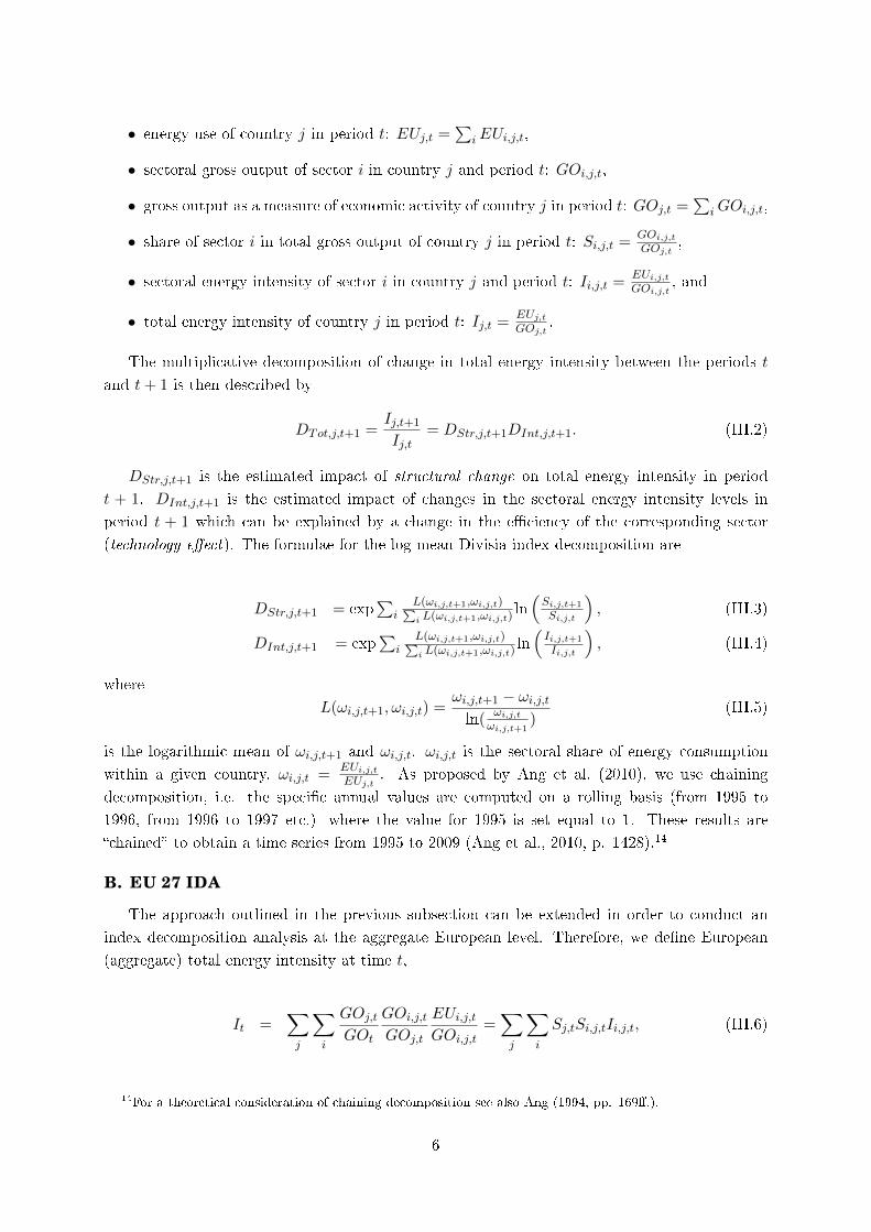
• energy use of country j in period t: EUj,t =∑

iEUi,j,t,

• sectoral gross output of sector i in country j and period t: GOi,j,t,

• gross output as a measure of economic activity of country j in period t: GOj,t =∑

iGOi,j,t,

• share of sector i in total gross output of country j in period t: Si,j,t =GOi,j,t

GOj,t,

• sectoral energy intensity of sector i in country j and period t: Ii,j,t =EUi,j,t

GOi,j,t, and

• total energy intensity of country j in period t: Ij,t =EUj,t

GOj,t.

The multiplicative decomposition of change in total energy intensity between the periods t

and t+ 1 is then described by

DTot,j,t+1 =Ij,t+1

Ij,t= DStr,j,t+1DInt,j,t+1. (III.2)

DStr,j,t+1 is the estimated impact of structural change on total energy intensity in period

t + 1. DInt,j,t+1 is the estimated impact of changes in the sectoral energy intensity levels in

period t + 1 which can be explained by a change in the e�ciency of the corresponding sector

(technology e�ect). The formulae for the log mean Divisia index decomposition are

DStr,j,t+1 = exp∑

iL(ωi,j,t+1,ωi,j,t)∑i L(ωi,j,t+1,ωi,j,t)

ln(Si,j,t+1

Si,j,t

), (III.3)

DInt,j,t+1 = exp∑

iL(ωi,j,t+1,ωi,j,t)∑i L(ωi,j,t+1,ωi,j,t)

ln(Ii,j,t+1

Ii,j,t

), (III.4)

where

L(ωi,j,t+1, ωi,j,t) =ωi,j,t+1 − ωi,j,tln(

ωi,j,t

ωi,j,t+1)

(III.5)

is the logarithmic mean of ωi,j,t+1 and ωi,j,t. ωi,j,t is the sectoral share of energy consumption

within a given country, ωi,j,t =EUi,j,t

EUj,t. As proposed by Ang et al. (2010), we use chaining

decomposition, i.e. the speci�c annual values are computed on a rolling basis (from 1995 to

1996, from 1996 to 1997 etc.) where the value for 1995 is set equal to 1. These results are

�chained� to obtain a time series from 1995 to 2009 (Ang et al., 2010, p. 1428).14

B. EU 27 IDA

The approach outlined in the previous subsection can be extended in order to conduct an

index decomposition analysis at the aggregate European level. Therefore, we de�ne European

(aggregate) total energy intensity at time t,

It =∑j

∑i

GOj,tGOt

GOi,j,tGOj,t

EUi,j,tGOi,j,t

=∑j

∑i

Sj,tSi,j,tIi,j,t, (III.6)

14For a theoretical consideration of chaining decomposition see also Ang (1994, pp. 169�.).

6

with the additional notation:

• EU27's energy use in period t: EUt =∑

j EUj,t,

• total EU27's gross output in period t: GOt =∑

j GOj,t,

• share of country j in total EU27's gross output in period t: Sj,t =GOj,t

GOt, and

• total EU27's energy intensity in period t: It = EUtGOt

.

This enables us to perform a three factor decomposition at the European level analogous to

equation III.2,

DTot,t+1 =It+1

It= DbStr,t+1DwStr,t+1DInt,t+1. (III.7)

In this case, we distinguish two aspects of structural change, a between-country structural

e�ect, DbStr,t+1, and a within-country structural e�ect, DwStr,t+1. An increase of the former

e�ect corresponds to a shift of the European economy toward more energy-intensive countries.

On the other hand, an increase in the latter e�ect denotes a shift toward more energy-intensive

sectors within the EU. The European technology e�ect, DInt,t+1, describes the overall energy

e�ciency change aggregated over each sector and each country. The corresponding formulae for

the log mean Divisia index decomposition are

DbStr,t+1 = exp∑

j

∑i

L(ω̃i,j,t+1,ω̃i,j,t)∑j

∑i L(ω̃i,j,t+1,ω̃i,j,t)

ln(Sj,t+1

Sj,t

), (III.8)

DwStr,t+1 = exp∑

j

∑i

L(ω̃i,j,t+1,ω̃i,j,t)∑j

∑i L(ω̃i,j,t+1,ω̃i,j,t)

ln(Si,j,t+1

Si,j,t

), (III.9)

DInt,t+1 = exp∑

j

∑i

L(ω̃i,j,t+1,ω̃i,j,t)∑j

∑i L(ω̃i,j,t+1,ω̃i,j,t)

ln(Ii,j,t+1

Ii,j,t

). (III.10)

The logarithmic mean L(ω̃i,j,t+1, ω̃i,j,t) is de�ned analogously to equation III.5, but ωi,j,t has

to replaced by the more �ne-grained parameter ω̃i,j,t describing the share of energy use of each

country and sector within European energy use, ω̃i,j,t =EUi,j,t

EUt. Also in this case we apply

chaining decomposition.

C. DECOMPOSING ENERGY INTENSITY ON A COUNTRY-LEVEL

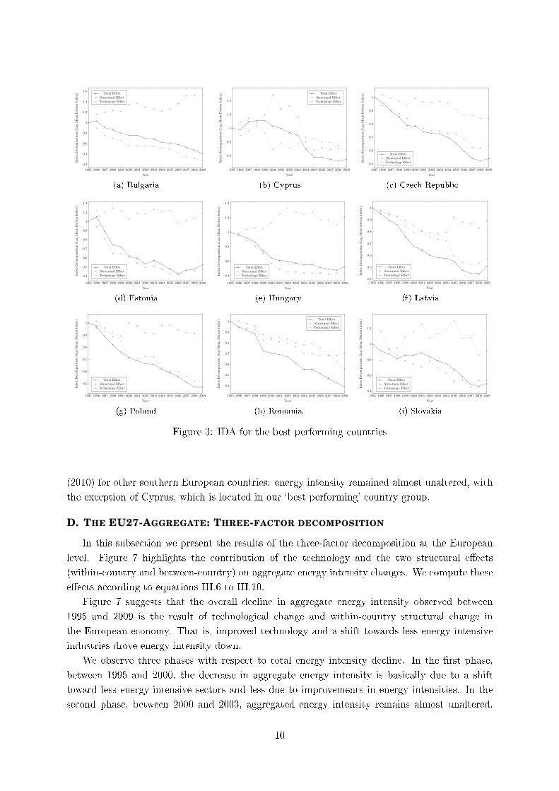
In this section, we perform the index decomposition on the individual European countries.

Figure 2 presents the annual growth rates of gross output and energy use (both in %) between

1995 and 2009. The dotted lines represent the respective EU27 averages. Eastern European

countries performed best (located in the lower right corner, implying above-average rises in gross

output and below-average rises in energy use), while some of Europe most mature countries

performed worst (located in the upper left corner, implying above-average rises in energy use

and below-average rises in gross output).

We use Figure 2 to identify four country groups. Our summary of the results will be brief

- most graphs tell their own tale - but we will take a moment to address some country-speci�c

7

0.5 1 1.5 2 2.5 3 3.5 4 4.5 5 5.5 6 6.5

−3

−2

−1

0

1

2

3

4

5

BGR

CYP

CZEESTHUN

LVA

POL

ROU

SVKFRA

GBR

DEU

ITANLD

SWE

EU27

IRL

LTU

LUX

AUTBEL

DNKESPFIN

GRC

MLTPRT

SVN

Growth Rate of Gross Output in % (Ø is dotted)

Growth

Rate

ofEnergyUse

in%

(Øis

dotted)

Best Countries

Medium I (- GO-Growth + EU-Growth)

Medium II (+ GO-Growth - EU-Growth)Worst Countries

Figure 2: GO- and EU-Growth

peculiarities and refer the reader to the work of authors who delved into more detail. Our regional

classi�cation based on output and energy use growth for the 27 European countries is as follows:

• Best Countries (Above Ø Output Growth, below Ø Energy Use Growth): Bulgaria,

Cyprus, Czech Republic, Estonia, Hungary, Latvia, Poland, Romania, Slovakia

• Medium I (Below Ø Output Growth, below Ø Energy Use Growth): France, Germany,

Italy, Netherlands, Sweden, United Kingdom

• Medium II (Above Ø Output Growth, above Ø Energy Use Growth): Ireland, Lithuania,

Luxembourg

• Worst Countries (Below Ø Output Growth, above Ø Energy Use Growth): Austria, Bel-

gium, Denmark, Finland, Greece, Malta, Portugal, Slovenia, Spain

Best Countries

The `best performing' group consists of Bulgaria, Cyprus, the Czech Republic, Estonia, Hun-

gary, Latvia, Poland, Romania and Slovakia. All countries are characterized by an above-average

rise in gross output and a below-average rise in energy use between 1995 and 2009.

Astonishingly, all countries save Cyprus are Eastern European. What is interesting about

these countries is that they experienced the largest structural change in our sample. Cornillie

and Fankhauser (2004) identi�ed a decoupling of energy use and economic activity in the Baltic

8

States (Estonia, Latvia and Lithuania) between 1992 and 1998. We can con�rm this trend for

Latvia and Estonia, though not for Lithuania, which is part of the Medium II country group

(above-average rises in gross output, above-average rises in Energy Use). But while Latvia's

improved energy intensity owed itself to better technology, the improvement in Estonia was

driven by less energy-intensive production. Our results are in line with Balezentisa et al. (2011),

who o�er a detailed discussion of the policy measures that a�ected the development in Lithuania,

notably the investments in modernizing buildings. Another example of improvement is Poland.

As Gurgul and Lach (2012) note, in the past decade Poland's economic growth has been tied

to changes in electricity utilization and to new, more energy-e�cient technologies in the face

of international environmental policy requirements. Romania and Bulgaria also experienced

dramatically improved energy e�ciency. As Popovici (2011) observed, �[t]he Romanian economy

was in 1990 one of the most energy-intensive in the region - only Bulgaria's economy was more

energy-intensive - due to the obsolete technologies [. . . ] that were energy-intensive and had

to import an increasing part of their raw materials. Due to the closure, technology upgrading

and restructuring in the heavy industries, Romania is nowadays much less energy intensive�

(Popovici, 2011, p. 1845). These economies experienced the largest structural change as also

shown by other recent studies (Mulder and De Groot, 2012).

Medium I

The second country group is characterized by above-average growth in gross output and an

above-average growth in energy use. It consists of France, Germany, Italy, Netherlands, Sweden

and the United Kingdom, all mature European economies.

France and the Netherlands show a continuous decline in overall energy intensity, but while

the economy in France shifted towards a more energy-intensive production, the economic com-

position in the Netherlands remained almost unaltered. The German economy moved towards

more energy-intensive production, resulting in a 7% increase in the structural change index. Yet

this e�ect is dominated by industrial improvement, as the nearly 30% decline in the technology

index shows. The United Kingdom and Sweden are examples for countries, where both e�ects

are decreasing, resulting in an overall energy intensity improvement of almost 40%.

The moderate energy intensity reductions in these countries is likely due to their mature

status as economies.

Medium II

The third country group is characterized by below-average growth in gross output and below-

average growth in energy use. It consists of three small counties: Ireland, Lithuania and Lux-

embourg. Lithuania is the only Eastern European country, besides Slovenia, that is not located

in the best performing country group.

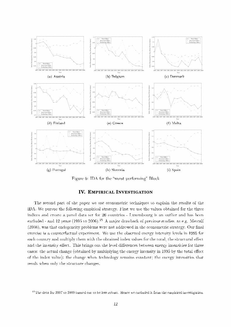
Worst Countries

Our �nal group consists of countries that performed below the European average in both

categories: Austria, Belgium, Denmark, Finland, Greece, Malta, Portugal, Slovenia and Spain.

Mendiluce et al. (2010) compared the evolution of energy intensity in Spain with 15 other Eu-

ropean countries (including Portugal and Greece). Our analysis con�rmed their �nding that

Spain's energy intensity reached its highest level in 2004. Thereafter it declined, mainly due to

the sharp decrease in the technology e�ect. We also con�rmed the �ndings of Mendiluce et al.

9

1995 1996 1997 1998 1999 2000 2001 2002 2003 2004 2005 2006 2007 2008 2009

0.2

0.4

0.6

0.8

1

1.2

1.4

1.6

Year

Ind

exD

ecom

pos

itio

n(L

ogM

ean

Div

isia

Index

) Total EffectStructural EffectTechnology Effect

Figure 1: Bulgaria(a) Bulgaria

1995 1996 1997 1998 1999 2000 2001 2002 2003 2004 2005 2006 2007 2008 2009

0.6

0.8

1

1.2

1.4

Year

Ind

exD

ecom

pos

itio

n(L

ogM

ean

Div

isia

Index

) Total EffectStructural EffectTechnology Effect

Figure 1: Cyprus(b) Cyprus

1995 1996 1997 1998 1999 2000 2001 2002 2003 2004 2005 2006 2007 2008 2009

0.5

0.6

0.7

0.8

0.9

1

Year

Ind

exD

ecom

pos

itio

n(L

ogM

ean

Div

isia

Index

)

Total EffectStructural EffectTechnology Effect

Figure 1: Czech Republic(c) Czech Republic

1995 1996 1997 1998 1999 2000 2001 2002 2003 2004 2005 2006 2007 2008 2009

0.4

0.5

0.6

0.7

0.8

0.9

1

1.1

1.2

Year

Index

Dec

omp

osit

ion

(Log

Mea

nD

ivis

iaIn

dex

)

Total EffectStructural EffectTechnology Effect

Figure 1: Estonia(d) Estonia

1995 1996 1997 1998 1999 2000 2001 2002 2003 2004 2005 2006 2007 2008 2009

0.4

0.6

0.8

1

1.2

1.4

Year

Index

Dec

omp

osit

ion

(Log

Mea

nD

ivis

iaIn

dex

)

Total EffectStructural EffectTechnology Effect

Figure 1: Hungary(e) Hungary

1995 1996 1997 1998 1999 2000 2001 2002 2003 2004 2005 2006 2007 2008 20090.4

0.5

0.6

0.7

0.8

0.9

1

Year

Index

Dec

omp

osit

ion

(Log

Mea

nD

ivis

iaIn

dex

)

Total EffectStructural EffectTechnology Effect

Figure 1: Latvia(f) Latvia

1995 1996 1997 1998 1999 2000 2001 2002 2003 2004 2005 2006 2007 2008 2009

0.5

0.6

0.7

0.8

0.9

1

Year

Index

Dec

omp

osit

ion

(Log

Mea

nD

ivis

iaIn

dex

)

Total EffectStructural EffectTechnology Effect

Figure 1: Austria(g) Poland

1995 1996 1997 1998 1999 2000 2001 2002 2003 2004 2005 2006 2007 2008 2009

0.4

0.5

0.6

0.7

0.8

0.9

1

Year

Index

Dec

omp

osit

ion

(Log

Mea

nD

ivis

iaIn

dex

) Total EffectStructural EffectTechnology Effect

Figure 1: Romania(h) Romania

1995 1996 1997 1998 1999 2000 2001 2002 2003 2004 2005 2006 2007 2008 2009

0.4

0.6

0.8

1

1.2

Year

Index

Dec

omp

osit

ion

(Log

Mea

nD

ivis

iaIn

dex

)

Total EffectStructural EffectTechnology Effect

Figure 1: Slovakia(i) Slovakia

Figure 3: IDA for the best performing countries

(2010) for other southern European countries: energy intensity remained almost unaltered, with

the exception of Cyprus, which is located in our `best performing' country group.

D. THE EU27-AGGREGATE: THREE-FACTOR DECOMPOSITION

In this subsection we present the results of the three-factor decomposition at the European

level. Figure 7 highlights the contribution of the technology and the two structural e�ects

(within-country and between-country) on aggregate energy intensity changes. We compute these

e�ects according to equations III.6 to III.10.

Figure 7 suggests that the overall decline in aggregate energy intensity observed between

1995 and 2009 is the result of technological change and within-country structural change in

the European economy. That is, improved technology and a shift towards less energy-intensive

industries drove energy intensity down.

We observe three phases with respect to total energy intensity decline. In the �rst phase,

between 1995 and 2000, the decrease in aggregate energy intensity is basically due to a shift

toward less energy-intensive sectors and less due to improvements in energy intensities. In the

second phase, between 2000 and 2003, aggregated energy intensity remains almost unaltered.

10

1995 1996 1997 1998 1999 2000 2001 2002 2003 2004 2005 2006 2007 2008 2009

0.6

0.7

0.8

0.9

1

1.1

1.2

Year

Ind

exD

ecom

pos

itio

n(L

ogM

ean

Div

isia

Index

)

Total EffectStructural EffectTechnology Effect

Figure 1: France(a) France

1995 1996 1997 1998 1999 2000 2001 2002 2003 2004 2005 2006 2007 2008 20090.7

0.75

0.8

0.85

0.9

0.95

1

1.05

1.1

Year

Ind

exD

ecom

pos

itio

n(L

ogM

ean

Div

isia

Index

)

Total EffectStructural EffectTechnology Effect

Figure 1: Germany(b) Germany

1995 1996 1997 1998 1999 2000 2001 2002 2003 2004 2005 2006 2007 2008 2009

0.7

0.8

0.9

1

1.1

1.2

Year

Ind

exD

ecom

pos

itio

n(L

ogM

ean

Div

isia

Index

)

Total EffectStructural EffectTechnology Effect

Figure 1: Italy(c) Italy

1995 1996 1997 1998 1999 2000 2001 2002 2003 2004 2005 2006 2007 2008 2009

0.7

0.75

0.8

0.85

0.9

0.95

1

1.05

Year

Index

Dec

omp

osit

ion

(Log

Mea

nD

ivis

iaIn

dex

)

Total EffectStructural EffectTechnology Effect

Figure 1: Austria(d) Netherlands

1995 1996 1997 1998 1999 2000 2001 2002 2003 2004 2005 2006 2007 2008 2009

0.65

0.7

0.75

0.8

0.85

0.9

0.95

1

1.05

Year

Index

Dec

omp

osit

ion

(Log

Mea

nD

ivis

iaIn

dex

)

Total EffectStructural EffectTechnology Effect

Figure 1: Sweden(e) Sweden

1995 1996 1997 1998 1999 2000 2001 2002 2003 2004 2005 2006 2007 2008 20090.6

0.7

0.8

0.9

1

Year

Index

Dec

omp

osit

ion

(Log

Mea

nD

ivis

iaIn

dex

)

Total EffectStructural EffectTechnology Effect

Figure 1: United Kingdom(f) United Kingdom

Figure 4: IDA for the Medium I Block

1995 1996 1997 1998 1999 2000 2001 2002 2003 2004 2005 2006 2007 2008 2009

0.6

0.7

0.8

0.9

1

1.1

1.2

Year

Index

Dec

om

posi

tion

(Log

Mea

nD

ivis

iaIn

dex

)

Total EffectStructural EffectTechnology Effect

Figure 1: Ireland(a) Ireland

1995 1996 1997 1998 1999 2000 2001 2002 2003 2004 2005 2006 2007 2008 2009

0.6

0.8

1

1.2

1.4

1.6

Year

Index

Dec

omp

osit

ion

(Log

Mea

nD

ivis

iaIn

dex

) Total EffectStructural EffectTechnology Effect

Figure 1: Lithuania(b) Lithuania

1995 1996 1997 1998 1999 2000 2001 2002 2003 2004 2005 2006 2007 2008 2009

0.7

0.75

0.8

0.85

0.9

0.95

1

Year

Index

Dec

om

posi

tion

(Log

Mea

nD

ivis

iaIn

dex

)

Total EffectStructural EffectTechnology Effect

Figure 1: Luxembourg(c) Luxembourg

Figure 5: IDA for the Medium II Block

The indices for the within-country structural events and the technology e�ects remain stable.

The between-country structural e�ects starts to rise, stating a shift of production towards more

energy-intensive countries. The third phase from 2003 to 2009 is characterized by a sharply

declining technology e�ect. It went down from 0.92 to 0.77. The within-country structural

e�ect remains stable, while the between-country structural e�ect rises to almost 1.05. Put it

otherwise, the energy-intensive sectors remained equal while energy-intensive countries gained in

importance. In combination, energy intensity declined in the period from 2003 to 2009 from 0.85

to 0.72, highlighting the importance of the technology e�ect. The development of this e�ect is

the key driver for the decline in total energy intensity.

Figure 10 in the appendix depicts the energy intensity evolution by sector between 1995 and

2009. While some sectors experience an increase in energy intensity - the energy intensity of

the wood and cork production ("Sector 20") increased by 33 % - most sectors experienced a

decrease. The decline ranged from moderate (-3.8 % in the inland transport, or sector "60")

to tremendous (-56.1 % in the coke, re�ned petroleum and nuclear fuel, or sector "23", an

energy-sector correlate).

11

1995 1996 1997 1998 1999 2000 2001 2002 2003 2004 2005 2006 2007 2008 2009

0.75

0.8

0.85

0.9

0.95

1

1.05

Year

Ind

exD

ecom

pos

itio

n(L

ogM

ean

Div

isia

Index

)

Total EffectStructural EffectTechnology Effect

Figure 1: Austria(a) Austria

1995 1996 1997 1998 1999 2000 2001 2002 2003 2004 2005 2006 2007 2008 2009

0.85

0.9

0.95

1

1.05

1.1

Year

Ind

exD

ecom

pos

itio

n(L

ogM

ean

Div

isia

Index

) Total EffectStructural EffectTechnology Effect

Figure 1: Belgium(b) Belgium

1995 1996 1997 1998 1999 2000 2001 2002 2003 2004 2005 2006 2007 2008 2009

0.85

0.9

0.95

1

1.05

1.1

1.15

Year

Ind

exD

ecom

pos

itio

n(L

ogM

ean

Div

isia

Index

) Total EffectStructural EffectTechnology Effect

Figure 1: Denmark(c) Denmark

1995 1996 1997 1998 1999 2000 2001 2002 2003 2004 2005 2006 2007 2008 2009

0.7

0.75

0.8

0.85

0.9

0.95

1

1.05

Year

Index

Dec

omp

osit

ion

(Log

Mea

nD

ivis

iaIn

dex

)

Total EffectStructural EffectTechnology Effect

Figure 1: Finland(d) Finland

1995 1996 1997 1998 1999 2000 2001 2002 2003 2004 2005 2006 2007 2008 2009

0.85

0.9

0.95

1

1.05

1.1

Year

Index

Dec

omp

osit

ion

(Log

Mea

nD

ivis

iaIn

dex

)

Total EffectStructural EffectTechnology Effect

Figure 1: Greece(e) Greece

1995 1996 1997 1998 1999 2000 2001 2002 2003 2004 2005 2006 2007 2008 2009

0.6

0.8

1

1.2

Year

Index

Dec

omp

osit

ion

(Log

Mea

nD

ivis

iaIn

dex

)

Total EffectStructural EffectTechnology Effect

Figure 1: Malta(f) Malta

1995 1996 1997 1998 1999 2000 2001 2002 2003 2004 2005 2006 2007 2008 2009

0.6

0.8

1

1.2

1.4

1.6

Year

Index

Dec

omp

osit

ion

(Log

Mea

nD

ivis

iaIn

dex

) Total EffectStructural EffectTechnology Effect

Figure 1: Portugal(g) Portugal

1995 1996 1997 1998 1999 2000 2001 2002 2003 2004 2005 2006 2007 2008 2009

0.7

0.8

0.9

1

1.1

1.2

Year

Index

Dec

om

posi

tion

(Log

Mea

nD

ivis

iaIn

dex

)

Total EffectStructural EffectTechnology Effect

Figure 1: Slovenia(h) Slovenia

1995 1996 1997 1998 1999 2000 2001 2002 2003 2004 2005 2006 2007 2008 2009

0.7

0.8

0.9

1

1.1

1.2

Year

Index

Dec

om

posi

tion

(Log

Mea

nD

ivis

iaIn

dex

)

Total EffectStructural EffectTechnology Effect

Figure 1: Spain(i) Spain

Figure 6: IDA for the �worst performing� Block

IV. EMPIRICAL INVESTIGATION

The second part of the paper we use econometric techniques to explain the results of the

IDA. We pursue the following empirical strategy. First we use the values obtained for the three

indices and create a panel data set for 26 countries - Luxembourg is an outlier and has been

excluded - and 12 years (1995 to 2006).15 A major drawback of previous studies, as e.g. Metcalf

(2008), was that endogeneity problems were not addressed in the econometric strategy. Our �nal

exercise is a counterfactual experiment. We use the observed energy intensity levels in 1995 for

each country and multiply them with the obtained index values for the total, the structural e�ect

and the intensity e�ect. This brings out the level di�erences between energy intensities for three

cases: the actual change (obtained by multiplying the energy intensity in 1995 by the total e�ect

of the index value); the change when technology remains constant; the energy intensities that

result when only the structure changes.

15The data for 2007 to 2009 turned out to be less robust. Hence we excluded it from the empirical investigation.

12

1995 1996 1997 1998 1999 2000 2001 2002 2003 2004 2005 2006 2007 2008 20090.7

0.75

0.8

0.85

0.9

0.95

1

1.05

Year

Index

Dec

om

pos

itio

n(L

og

Mea

nD

ivis

iaIn

dex

)

Total Effect

Structural Effect (between)

Structural Effect (within)Technology Effect

Figure 7: Log Mean Divisia Index Decomposition of Energy Intensity

A. MODEL AND VARIABLES

We estimate three similar panel models by index type for the dependent variables (x ∈(DTot, DStr, DInt)). Our indices control for in�uential factors, measuring the real decline in

energy intensity, the fraction caused by structural change, and the contribution of technology.

Our estimation model is expressed by the following equation:

Indexxjt = = β0 + βXjt + δZjt + εjt (IV.11)

with x ∈ (DTot, DStr, DInt)

βXjt as major covariates,

δZjt as additional controls, and

εjt as an idiosyncratic error term.

13

We estimate the following equations:

Indexxjt = β0 + β1INCOMEjt + β2INCOMESQRjt + β3OPENjt + (IV.12)

+β4K/Ljt + β5K/LSQRjt + β6MANUFACSHAREjt +

+β7TFPjt + β8ENERGYPRICEjt + β9REGULjt +

+δ1VINTAGINGjt + δ2AREAjt + δ3POPGROWTHjt +

+δ4LATITUDEj + δ5HDDjt + δ6COMMUNISTj +

+δ7RENEWABLESHAREjt + δ8TRENDjt + δ9TRENDSQRjt +

+εjt

with x ∈ (DTot, DStr, DInt)

The variables are:

• INCOME = Instrumented Income per Capita (logarithmic)

• INCOMESQR = Income per Capita squared (logarithmic)

• OPEN = Instrumented Trade Openness (logarithmic)

• K/L = Capital to Labor Ratio (logarithmic)

• K/LSQR = Capital to Labor Ratio squared (logartihmic)

• MANUFACSHARE = Share of Manufacturing (logarithmic)

• TFP = Estimated Total Factor Productivity (logarithmic and in di�erences)

• ENERGYPRICE = Price of Energy (logarithmic)

• REGUL = Index of Energy E�ciency Regulation

• VINTAGING = Capital Vintaging (logarithmic)

• AREA = Area of Country (logarithmic)

• POPGROWTH = Population Growth Rate

• LATITUDE = Latitude of the Country

• HDD = Heating Degree Days (logarithmic)

• COMMUNIST = Dummy = 1 for former communist countries

• RENEWABLESHARE = Share of �green� energy in total energy use (logarithmic)

• TREND = Control variable for time trend

• TRENDSQR = Control variable for time trend squared

Before presenting our results, we discuss and justify the variables. Our model consists of 15

variables (and a control for a time trend) attributable to various e�ects.

14

Income

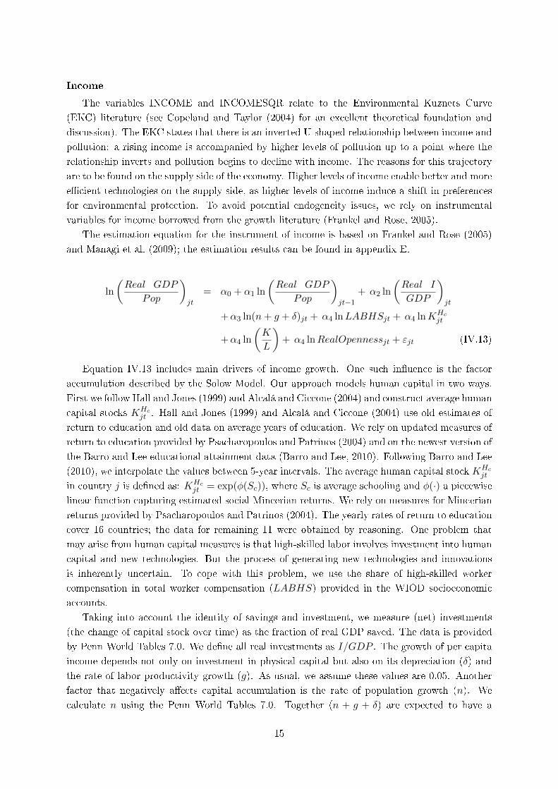
The variables INCOME and INCOMESQR relate to the Environmental Kuznets Curve

(EKC) literature (see Copeland and Taylor (2004) for an excellent theoretical foundation and

discussion). The EKC states that there is an inverted U-shaped relationship between income and

pollution: a rising income is accompanied by higher levels of pollution up to a point where the

relationship inverts and pollution begins to decline with income. The reasons for this trajectory

are to be found on the supply side of the economy. Higher levels of income enable better and more

e�cient technologies on the supply side, as higher levels of income induce a shift in preferences

for environmental protection. To avoid potential endogeneity issues, we rely on instrumental

variables for income borrowed from the growth literature (Frankel and Rose, 2005).

The estimation equation for the instrument of income is based on Frankel and Rose (2005)

and Managi et al. (2009); the estimation results can be found in appendix E.

ln

(Real_GDP

Pop

)jt

= α0 + α1 ln

(Real_GDP

Pop

)jt−1

+ α2 ln

(Real_I

GDP

)jt

+α3 ln(n+ g + δ)jt + α4 lnLABHSjt + α4 lnKHcjt

+α4 ln

(K

L

)+ α4 lnRealOpennessjt + εjt (IV.13)

Equation IV.13 includes main drivers of income growth. One such in�uence is the factor

accumulation described by the Solow Model. Our approach models human capital in two ways.

First we follow Hall and Jones (1999) and Alcalá and Ciccone (2004) and construct average human

capital stocks KHcjt . Hall and Jones (1999) and Alcalá and Ciccone (2004) use old estimates of

return to education and old data on average years of education. We rely on updated measures of

return to education provided by Psacharopoulos and Patrinos (2004) and on the newest version of

the Barro and Lee educational attainment data (Barro and Lee, 2010). Following Barro and Lee

(2010), we interpolate the values between 5-year intervals. The average human capital stock KHcjt

in country j is de�ned as: KHcjt = exp(φ(Sc)), where Sc is average schooling and φ(·) a piecewise

linear function capturing estimated social Mincerian returns. We rely on measures for Mincerian

returns provided by Psacharopoulos and Patrinos (2004). The yearly rates of return to education

cover 16 countries; the data for remaining 11 were obtained by reasoning. One problem that

may arise from human capital measures is that high-skilled labor involves investment into human

capital and new technologies. But the process of generating new technologies and innovations

is inherently uncertain. To cope with this problem, we use the share of high-skilled worker

compensation in total worker compensation (LABHS) provided in the WIOD socioeconomic

accounts.

Taking into account the identity of savings and investment, we measure (net) investments

(the change of capital stock over time) as the fraction of real GDP saved. The data is provided

by Penn World Tables 7.0. We de�ne all real investments as I/GDP . The growth of per capita

income depends not only on investment in physical capital but also on its depreciation (δ) and

the rate of labor productivity growth (g). As usual, we assume these values are 0.05. Another

factor that negatively a�ects capital accumulation is the rate of population growth (n). We

calculate n using the Penn World Tables 7.0. Together (n + g + δ) are expected to have a

15

negative impact on income per capita. Following Managi et al. (2009) we also control for the

(logarithmic) capital-to-labor ratio KL and (logarithmic) real openness RealOpenness.

We expect that the coe�cient for INCOME will be positive and the coe�cient for IN-

COMESQR will be negative in the case of DTot and DInt. This implies higher index values

for higher incomes until the peak of the EKC is reached and then a lower index value for higher

rates of income.

Trade

The next variable is OPEN, de�ned as the sum of export and imports divided by real gross

output in 1995 in US-$:

Openessjkt =Xjkt +Mjkt

GOjtREALj,1995; j 6= k (IV.14)

The gravity equation for the geography-based bilateral trade share of two countries j and k is

borrowed from the work of Frankel and Romer (1999) and Frankel and Rose (2005):

lnOpenessjkt = γ0 + γ1 lnDistancejk + γ2 lnPopjt + γ3 lnPopkt

+ γ4 lnAreajt + γ5 lnAreakt + γ6(LLjt + LLkt) + γ7CBjkt (IV.15)

+ γ8CBjkt lnDistancejkt + γ9CBjkt lnPopjt + γ10CBjkt lnPopkt

+ γ11CBjkt lnAreajt + γ12CBjkt lnAreakt + γ13CBjkt(LLjt + LLkt) + εjkt

The regressor Djkt represents the geographic distance between the capitals of the two trade

partners j and k. Popjt and Popkt are measures of population in countries j and k, respectively.

In contrast to Frankel and Romer (1999), the measures do not cover the economically active

population on account of missing data for some countries in the Penn World Tables. Areajt and

Areakt are controls for the size of two countries; LLjt and LLkt are dummies measuring whether

the countries are landlocked. LLjt +LLkt is the common landlocked dummy, which summarizes

dummies representing landlocked status. The variable CBjkt is a dummy that assumes the value

of 1 when trade partners share a common border. The common border dummy is interacted with

other explanatory variables to capture trade between neighboring countries more accurately. The

equation is estimated by means of least squares, using the bilateral trade data for all countries

included in the WIOD. The geographical information was obtained from the CIA World Fact

Book and from the CEEPI Gravity Data Set (Meyer, 2011). After estimating the (�rst stage)

regression to construct the instrument for trade openness, we aggregate the �tted values across

all bilateral trade partners. The aggregation yields a given country's trade openness adjusted

according to output-based PPPs. The aggregation method is presented in equation D21:

ˆOpenessjt =∑j 6=k

eγ̂′Xjkt (IV.16)

The vector γ represents the coe�cients in equation IV.15 whereas the vector Xjkt stands for

the right-hand side variables in equation IV.15. From the �rst regression on, �tted values were

used to predict trade openness. The results of the main regression are shown in Table 7. We

had to run the regression for each year to get meaningful data because each geography variable

16

is remains the same over time. Consequently, treating trade �ows as a single observation would

yield almost constant trade openness observations. The only way to solve the problem is to run

the regression individually for each year. This procedure produces the correct predicted trade

openness values with time variation - values we later need for our instruments.16

As Antweiler et al. (2001) demonstrate in their seminal paper, trade can have a signi�cant

and positive impact on the environment through its e�ects on income and economic composition.

And when it does, we can expect that trade will also have a signi�cant indirect e�ect on the

economy's energy intensity. Accordingly, we expect the OPEN coe�cient to be negative for all

three indicators.

Capital-to-Labor Ratio and Manufacturing Share

The capital to labor ratio K/L is also relevant for the structure of the economy under in-

vestigation. We adopt the assumption of Antweiler et al. (2001) that greater capital intensity

correlates with greater pollution and energy use (see also Cole and Elliott (2003) and Cole

(2006) for further evidence). The WIOD has sectoral estimates for physical capital stocks for all

countries and periods. These estimates allow us to test the hypothesis that an increasing capital-

to-labor ratio (an indirect measure of structural change) results in increasing energy intensity.

We calculate the sample mean of the capital-to-labor ratio and then use relative capital-to-labor

ratios. We believe that this concept is superior to Metcalf's , for it accounts not only for struc-

tural change but also for comparative advantages between countries. The correlation between

total energy use and capital intensity (measured in physical capital stock per working hour) is

0.44 and statistically signi�cant on the 1 % level for our 27-country sample. We expect a negative

coe�cient for the K/L variable for DStr. Another important control for structural change is the

share of the secondary (manufacturing) block in an economy. We subtract the gross out of agri-

culture, mining and services from total gross output and use this as the share of manufacturing

industries (MANUFACSHARE).

Total Factor Productivity

The next variable is the estimated total factor productivity (TFP). Syverson (2011) reports in

his survey that even within U.S. four-digit SIC industries, the (average) di�erence in logarithmic

multifactor productivity between an industry's 90th and 10th percentile plants is .651, resulting

in a TFP ratio of e.651 = 1.92. That means that, even within a single four-digit SIC industry

in a single country, the 90th percentile of the productivity distribution produces almost twice as

much output with the same inputs as the 10th percentile plant. Comin et al. (2006) investigate

direct measures of technology adoption for more than 75 di�erent technologies and demonstrate

that the cross-country di�erences in technology are roughly four times larger than cross-country

di�erences in income per capita and that technology is positively correlated to income per capita.

Thus, cross-country variation in TFP is almost solely determined by cross-country variation in

physical technology. As the European Union is a much more heterogeneous economic environment

than the United States, we argue that di�erences in total factor productivity growth are (a)

substantial by themselves and (b) have a substantial impact on energy utilization. We rely on a

16Sascha Rexhäuser o�ered us valuable insight about the procedure.

17

standard measure for gross-output-based TFP as presented in Hsieh and Klenow (2010).17 Level

accounting can be interpreted as the cousin of the traditional growth accounting introduced by

Robert Solow. Comparison studies of labor productivity often de�ne the United States as the

technology leader and then measure the distance between other countries and this reference value.

Because we are interested in changes in energy use technology, we use the country with the second-

lowest aggregate energy intensity in 1995 as the reference country (Austria and Luxembourg

had very similar here. We made an arbitrary decision for Austria). To estimate the total

factor productivity we use the gross-output and capital-to-output ratios from the WIOD. We

assume a share of capital of 0.3. To control for human capital, we combine these data with the

updated Barro and Lee dataset on educational attainment and information on Mincerian returns

to education provided by Psacharopoulos and Patrinos (2004).18 Our estimation equation for

TFP builds on Hall and Jones (1999); Alcalá and Ciccone (2004) and Hsieh and Klenow (2010)

and takes the form:

TFPjt =rgdpwok

( KGO · rgdpwok)α · exp(Θ · SchoolingYears))1−α

(IV.17)

We combine multiple data sources to obtain our TFP estimate. We start with real gdp per worker

from the Penn World Tables 7.0. K over GO describes the relationship of physical capital stock

to gross output as recorded in the WIOD. α refers to the share of capital compensation and is

taken to be 0.3, which is in line with common assumptions. Θ stands for Mincerian returns to

education, again taken from Psacharopoulos and Patrinos (2004). We combine this information

with our interpolated version of the Barro and Lee dataset, thus correcting the TFP measure

for human capital formation. To see how our measure for total factor performs, we calculated

the growth rates of TFP and instrumented income per capita and plotted them. The result is

presented in Figures 8a and 8b:

We include the TFP variable expressed in logs. We expect that the coe�cient will be negative

in the case of DTot and DInt, implying a lower index value for higher rates of total factor

productivity. The e�ect on the economic structure is unknown ex ante.

Regulation and Prices

The next variables are prices (ENERGYPRICE) and regulatory measures (REGUL). We

used the annual average energy prices as a measure for price induced changes in technology

or economic structure. The data source is Eurostat.19 We also collected data on environmental

regulation in the European Union for the time period under consideration. To account for various

climate and environmental policies, we made use of the Policies and Measures Databases provided

by the International Energy Agency (IEA, 2012). They consist of three di�erent databases:

Global Renewable Energy, Energy E�ciency, and Policy Measures Addressing Climate Change.

17Citing Hsieh and Klenow (2010) neglects many other important contributions dealing with multifactor pro-ductivity. For more here, see the surveys by Caselli (2005) and Syverson (2011).

18Psacharopoulos and Patrinos (2004) provides detailed information on Mincerian returns for 16 of our 27countries. For the remaining 11 countries, we use values from countries with similar economic and politicalstructures. For example, we apply the 6.4 % p.a. given for Belgium to the Netherlands.

19Of the 405 data points (spanning 27 countries and 15 years), 76 were missing, mostly from 1998. To createproxies for the absent data, we interpolated the values from 1997 and 1999.

18

1 1.5 2 2.5 3 3.50.3

0.4

0.5

0.6

0.7

0.8

0.9

1

ROUBGR

LVALTUPOL ESTPRT

CYPHUNSVK FRAMLT DEUCZE

ESPGRC

FINSVN

NLD

AUTIRLDNKGBR

BELSWE

ITA

Instrumented Income, 2007, in 10.000 US-$

Estim

atedTFP,20

07,Italy

=1.00

(a) TFP vs. Income

−1 0 1 2 3 4 5 6 7 8 9 10

2

4

6

8

10

BGR

CYP

CZE

EST

HUN

LVA

POL

ROU

SVK

FRAGBR

DEU

ITA

NLD

SWE

IRL

LTU

AUT

BELDNK

ESP

FIN

GRC

MLT

PRT

SVN

Growth Rate of Estimated TFP in 2007 in %

Growth

Rateof

InstrumentedIncomein

2007

%

BestMedium I + II

Worst

(b) TFP-Growth vs. Income-Growth

Figure 8: TFP vs. Instrumented Income and TFP-Growth vs. Income-Growth

Altogether, these databases contain data on more than 3,600 policies and on all types of policy

measures going back to 1973 for some 50 countries. The information recorded in the databases

encompasses indicators such as targeted sector (e.g. electricity, appliances, buildings, industry),

technology (with particular emphasis on renewable technologies), jurisdiction (whether the policy

is implemented on a subnational, national or international level) and policy type (e.g. R & D

investments, standards, taxes, permits).

We prepared the data in the following way. First, we merged the databases, creating a com-

mon ground for the regulatory stringency index. Second, we broke down policies containing

multiple indicators (e.g. solar PV/wind/bioenergy and R & D investments/standards) or poli-

cies assigned to multiple sectors into single policy measures. Sometimes this meant dropping

observations when our manual search found no speci�c information or indicator for a database

entry. We also dropped observations to avoid double counting, as some policies are reported in

more than one of the original databases. This left us with approximately 3,200 policy measures

for the analysis. Third, for the policy types and targeted technologies within the energy sector

we constructed multi-level structures in which we assigned the types and technologies appearing

in the original database to higher-level instances.20

We apply a weighting scheme for policy to construct our regulatory index. The various

energy policies can be subdivided into three di�erent groups, each characterizing a di�erent

level of stringency. First, there are technology-oriented measures such as voluntary approaches

and the subsidization of R & D. These are the least stringent measures in the construction of

our regulation index. The second group consists of command-and-control based policies such

as standards and quotas. And �nally, there are market-based instruments, which we classify

as most stringent. Though we conducted sensitivity analysis with various weighting schemes,

20We thank Enrica De Cian, Elena Verdolini and Sebastian Voigt for providing us with their data.

19

the results changed neither qualitatively nor quantitatively. Our index was constructed by the

following formula:

REGULjt = ω∑

TECHjt + θ∑

COMMANDjt +∑

φMARKETjt (IV.18)

with j ∈ 1, . . . , 27,

t ∈ 1995, . . . , 2006,

ω, θ andφ as weights

andTECHN, COMMAND andMARKET as policy types.

For our main estimations we used 0.5 for ω, 0.8 for θ and 1.0 for φ.21 Figure 9 illustrates

the development of our reference energy e�ciency regulation index for four countries: Germany,

Sweden, Poland and Slovenia. Two observations are remarkable. First, the index value is for

all mature European countries whose energy e�ciency is higher than that of Eastern European

countries. And second, an energy e�ciency trend can be found for Western countries but not for

Eastern. These two observations hold true for the entire sample and will be important for the

interpretation of the estimation results later in the paper.

1995 1996 1997 1998 1999 2000 2001 2002 2003 2004 2005 2006

0

2

4

6

8

10

12

Year

Regulatory

Index

GermanyPolandSloveniaSweden

Figure 9: Regulatory index for four countries

Further Controls

We also included several other control variables in our regression model. VINTAGING cap-

tures the national di�erences in capital stock vintaging (Source: WIOD). VINTAGING is in-

cluded in the model as the ratio of investment to capital stock. The e�ect may be positive since

fast growing countries may have newer capital stock, which uses less energy and is hence more

e�cient. AREA is the geographical area of a country in km2 taken from the CIA World Fact

Book. It captures the e�ects of potential economies of scale (Sala-i-Martin, 1997a,b). Larger

21We used vastly di�erent weighting schemes, ranging from equal weights to situations in which only command-and-control policies mattered (i.e. where ω and φ were 0). The results are insensitive to the choice of the weights.

20

countries may need larger but more e�cient power plants. On the other hand, these countries

may need larger power grids, which have lower e�ciency. POPGROWTH is the population

growth rate (see PWT 7.0). It captures the e�ect of a growing population on energy intensity, as

�fast growing states may be adding infrastructure that is more energy e�cient than slow grow-

ing states� (Metcalf, 2008, p. 9). Furthermore, as Kormendi and Meguire (1985) pointed out,

a fast growing population may hamper economic growth and therefore lower income per capita

and alter environmental preferences. The variable LATITUDE is the geographical latitude of

a country (see CIA World Fact Book) and might be an important driver of energy intensity to

be accounted for. The rationale behind the LATITUDE variable is twofold. First, southern

European countries such as Italy and Spain have a larger demand for power plant cooling and air

conditioning (in sectors outside the private sector) than central European countries. Conversely,

northern European countries such as Finland and Sweden have a larger demand for heating and

lighting than the rest of Europe. By including the LATITUDE of a country we control for this

e�ect. The second rationale behind the LATITUDE variable is that geographical latitude may be

a determinant of long-run economic development and growth (Rodrik et al., 2004). Accordingly,

it can also a�ect the environmental preferences expressed by the POPGROWTH variable. In

line with Metcalf (2008) we included heating demand days to control for climate factors.

The COMMUNIST variable is a dummy variable that equals 1 when a country was part of

the former Soviet block. The fall of the Iron Curtain brought with it a tremendous structural

break, rendering the old capital stock in these countries nearly worthless. In this case, the vin-

tage capital structure would be di�erent than that of the "old" European countries. Another

consideration is the �low-hanging fruits� for energy e�ciency in the former Soviet countries. Our

COMMUNIST dummy captures these e�ects. We also introduced a control for the regulation

index (REGUL). Because the regulation index measures current activities in energy e�ciency

policy, it might omit past e�orts. Hence, we calculate the share of renewable energy sources in

energy e�ciency policy using information on 26 energy carriers from WIOD. The variable RE-

NEWABLESHARE captures the e�orts of past regulatory measures and accounts for "natural"

endowments in renewable energy (such as those found in Sweden). Finally, we have included a

time trend in our regressions to capture independent in�uential factors we did not account for.

B. RESULTS AND INTERPRETATION

I. Empirical Approach

Our panel data sets a�ord two principle approaches for econometric modeling that can be

applied to any of our models: �xed-e�ects estimators and random-e�ects estimators. The key

advantage of using the �xed-e�ects estimator is that it typically includes dummy variables that

capture the in�uence of time-invariant, unobservable factors - topography, other country-speci�c

characteristics - that might be correlated with explanatory variables. The result: consistent

estimates. By contrast, the random-e�ects estimator assumes that a correlation with the regres-

sors is 0. When this assumption is met, the random-e�ects estimator is more e�cient than the

�xed-e�ects estimator. If this assumption is violated, however, the estimates will be biased. We

run both �xed- and random-e�ects estimators and apply the standard Hausman test to validate

which type of estimator is more appropriate (Wooldridge, 2002). Notwithstanding, the �gures

21

for the index decomposition might depict a kind of spurious correlation. Thus, we carry out unit

root tests for panel data. Herein, we focus on the Fisher-type Augmented Dickey Fuller test for

unit roots in panel data (based on Dickey and Fuller, 1979). The tests indicate a unit root in

the technology e�ect index variable, the income per capita variable and the heating degree days

variable. All other variables do not have unit roots according to the test results.

II. Results of our Core Model: Index Values as Dependent Variables

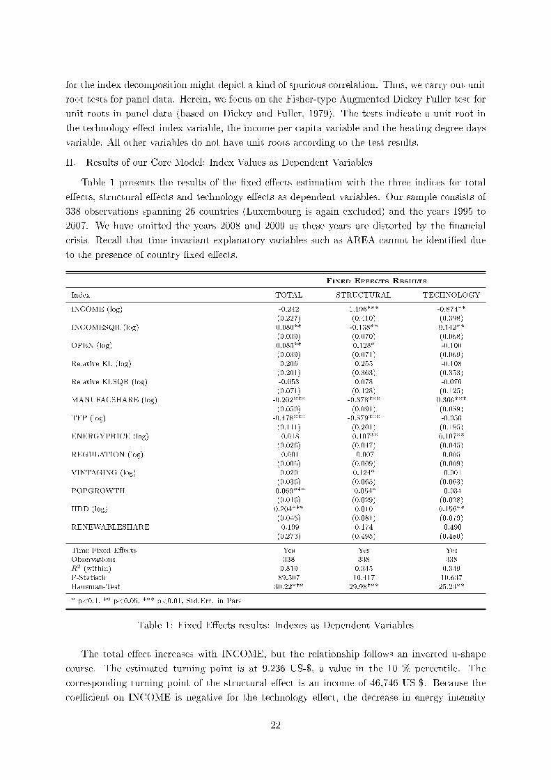
Table 1 presents the results of the �xed-e�ects estimation with the three indices for total

e�ects, structural e�ects and technology e�ects as dependent variables. Our sample consists of

338 observations spanning 26 countries (Luxembourg is again excluded) and the years 1995 to

2007. We have omitted the years 2008 and 2009 as these years are distorted by the �nancial

crisis. Recall that time-invariant explanatory variables such as AREA cannot be identi�ed due

to the presence of country �xed e�ects.

Fixed Effects Results

Index TOTAL STRUCTURAL TECHNOLOGY

INCOME (log) -0.242 1.196*** -0.874**(0.227) (0.410) (0.398)

INCOMESQR (log) 0.080** -0.138** 0.142**(0.039) (0.070) (0.068)

OPEN (log) 0.085** 0.128* -0.100(0.039) (0.071) (0.069)

Relative KL (log) 0.206 0.255 -0.108(0.201) (0.363) (0.353)

Relative KLSQR (log) -0.053 0.078 -0.076(0.071) (0.128) (0.125)

MANUFACSHARE (log) -0.202*** -0.378*** 0.366***(0.050) (0.091) (0.089)

TFP (log) -0.478*** -0.879*** -0.056(0.111) (0.201) (0.195)

ENERGYPRICE (log) -0.018 -0.107** 0.107**(0.026) (0.047) (0.045)

REGULATION (log) -0.001 -0.007 0.005(0.005) (0.009) (0.009)

VINTAGING (log) 0.020 0.124* -0.001(0.036) (0.065) (0.063)

POPGROWTH -0.069*** -0.054* -0.034(0.016) (0.029) (0.028)

HDD (log) 0.204*** 0.010 0.156**(0.045) (0.081) (0.079)

RENEWABLESHARE -0.199 0.174 -0.490(0.273) (0.495) (0.480)

Time Fixed E�ects Yes Yes YesObservations 338 338 338R2 (within) 0.819 0.345 0.349F-Statistic 89.507 10.417 10.637Hausman-Test 30.22*** 29.98*** 25.23**

* p<0.1, ** p<0.05, *** p<0.01, Std.Err. in Pars

Table 1: Fixed E�ects results: Indexes as Dependent Variables

The total e�ect increases with INCOME, but the relationship follows an inverted u-shape

course. The estimated turning point is at 9.236 US-$, a value in the 10 % percentile. The

corresponding turning point of the structural e�ect is an income of 46,746 US-$. Because the

coe�cient on INCOME is negative for the technology e�ect, the decrease in energy intensity

22

happens via the e�ciency channel. We conclude that scale e�ects are dominated by technology

e�ects, as a rising INCOME lowers aggregate energy intensities. This could be due to an increase

in environmental regulation (preference shifts) or the usage of more advanced technologies.

An increasing OPENNESS variable - an increasing participation in international trade -

lowers, ceteris paribus, the total energy intensity index. Because the coe�cient for the structural

e�ect is positive (implying higher values for the structural e�ect), the decrease in the total e�ect

is once again explained by the e�ciency channel. The corresponding coe�cient is even higher and

statistically signi�cant on the 1 %-level. This could be due to an outsourcing of energy-intensive

industries or imports of improved technology from abroad.

The total e�ect increases as the relative capital-to-labor ratio grows. The calculated turning

point is a capital-to-labor ratio of 3.79, a value above the maximum level of 3.59 for the capital-

to-labor ratio in the sample (note that the squared term is not signi�cant). The e�ect of an

increasing capital-to-labor ratio is not signi�cant in the regressions for the other two index

values. Hence, we can con�rm that capital and energy complement each other in the short run.

This �nding is supported by the coe�cient of VINTAGING. Countries with higher investment

rates tend to have higher energy intensity. Most important is the TFP variable, which represents

advantages in technology. Countries with higher growth rates in total factor productivity have,

ceteris paribus, lower energy intensities. Surprisingly, this occurs via the structural channel. Our

control variable for energy e�ciency regulation is not signi�cant in any model.

To summarize, the variables we declared important for technological change (INCOME, IN-

COMESQR and TFP) play the most crucial role in driving the decline in energy intensity, though

structural change factors (as e.g. OPEN, KL and KLSQR) are also relevant.

III. Results of our Core Model: Real Values as Dependent Variables

Our �nal empirical exercise is combining the energy intensity in 1995 with the obtained

index values for the three e�ects. By doing this, we take the level di�erences between energy

intensities into account. Hence, our dependent variables are no longer index values, but the three

logarithmic energy intensities. Table 2 summarizes the results of running our core model on the

three energy intensity levels:

23

Fixed Effects Results

Index TOTAL STRUCTURAL TECHNOLOGY

INCOME (log) -0.476* 1.185*** -1.718***(0.282) (0.436) (0.455)

INCOMESQR (log) 0.118** -0.144* 0.275***(0.048) (0.074) (0.078)

OPEN (log) 0.096** 0.293*** -0.203**(0.049) (0.075) (0.078)

Relative KL (log) 0.293 0.262 0.047(0.249) (0.386) (0.403)

Relative KLSQR (log) -0.085 0.113 -0.206(0.088) (0.136) (0.142)

MANUFACSHARE (log) -0.282*** -0.727*** 0.446***(0.063) (0.097) (0.101)

TFP (log) -0.661*** -0.908*** 0.239(0.138) (0.213) (0.223)

ENERGYPRICE (log) -0.041 -0.151*** 0.114**(0.032) (0.050) (0.052)

REGULATION (log) -0.001 -0.006 0.005(0.006) (0.010) (0.010)

VINTAGING (log) 0.023 0.107 -0.083(0.045) (0.069) (0.072)

POPGROWTH -0.090*** -0.062** -0.028(0.020) (0.030) (0.032)

HDD (log) 0.230*** 0.031 0.194**(0.056) (0.086) (0.090)

RENEWABLESHARE -0.444 0.061 -0.517(0.339) (0.525) (0.549)

Time Fixed E�ects Yes Yes YesObservations 338 338 338R2 (within) 0.834 0.485 0.421F-Statistic 99.307 18.662 14.389

* p<0.1, ** p<0.05, *** p<0.01, Std.Err. in Pars

Table 2: Fixed E�ects results: Levels as Dependent Variables

Regressing levels on the explanatory variables con�rms our previous results. Most of the

estimated parameters retain their direction and their signi�cance. INCOME and INCOMESQR,

for example, have signi�cant impacts on all three e�ects. Their magnitude is stronger when

explaining the total and the technology e�ect in levels than when explaining them in indexes.

Our measure of openness remains highly signi�cant, as do MANUFACSHARE and TFP.

V. CONCLUSION

The purpose of this study is to explain the forces driving improvements in energy intensity

in the European Union between 1995 and 2009, in times with and without climate policy and

economic turbulence. It contributes to the large literature on energy decomposition analysis

in three ways. First, it is the only analysis of energy intensity at country and sectoral levels

for the entire European Union using a perfect decomposition methodology. It employs a novel

socio-economic database escorted by environmental satellite accounts allowing us to construct

measures of energy intensity for 34 sectors in 27 countries. Second, this study uses econometric

methods to identify the drivers of changes in e�ciency and economic activity indexes. Third, it

carefully addresses endogeneity issues, an aspect that has been ignored by previous studies.

24

We decomposed energy intensities into structural and technology e�ects in order to examine

what share of temporal variation is due to changes in energy e�ciency and is thus replicable,

and what share is based merely on structural changes of the economy. We grouped the countries

in four main clusters with respect to gross output and energy use growth rates. Despite the

regional variations, the general result is that in most countries both the technology and structural

indexes improved over the time horizon considered. In some countries energy e�ciency improved

substantially, further below the already low initial levels in 1995. In this case, both the structural

and technology e�ects work in the direction of an energy e�cient economy.

The aggregate and country-level decompositions of energy intensity we have presented in

this paper suggest very di�erent conclusions. We �nd that technological advances are a main

explanatory factor for energy intensity improvement in Europe, suggesting a general transition

towards more e�cient means of production. Conversely, our country-level analysis shows that

the heterogeneity across countries is high and that a common pattern could not have been singled

out without an empirical investigation. Countries' performances in terms of the structural and

technology component di�er independently of the economy's level of development or initial level

of energy e�ciency. Among the di�erent economies in our sample, some large countries where

the role of the technology component was high include, among others, Germany, France, Spain

and Poland. This is an optimistic conclusion, as it means that the development is replicable in

less developed regions such as India or China. Although structural change is nearly as important

- no surprise after the fall of the Iron Curtain - technological progress is the key driving force.

25

REFERENCES

Alcalá, F., Ciccone, A. (2004): Trade and productivity, in: The Quarterly Journal ofEconomics, Vol. 119, No. 2, pp. 613-646.

Alcantara, V., Duarte, R. (2004): Comparison of energy intensities in European Unioncountries. Results of a structural decomposition analysis, in: Energy Policy, Vol. 32, pp. 177-189.

Ang, B.W. (1994): Decomposition of industrial energy consumption, in: Energy Economics,Vol. 16, pp. 163-174.

Ang, B.W., Choi, K.H. (1997): Decomposition of aggregate energy and gas emission inten-sitites for industry: a re�ned Divisia index method, in: The Energy Journal, Vol. 18, pp.59-73.

Ang, B.W., Zhang, F.Q., Choi, K.-H. (1998): Factorizing changes in energy and environ-mental indicators through decomposition, in: Energy, Vol. 23, pp. 489-495.

Ang, B.W., Zhang, F.Q. (2000): A survey of index decomposition analysis in energy andenvironmental studies, in: Energy, Vol. 25, pp. 1149-1176.

Ang, B.W. (2004): Decomposition analysis for policymaking in energy: which is the preferredmethod?, in: Energy Economics, Vol. 32, pp. 1131-1139.

Ang, B.W., Liu, N. (2007): Energy decomposition analysis: IEA model versus other methods,in: Energy Policy, Vol. 35, pp. 1426-1432.

Ang, B.W.,Mu, A.R., Zhou, P. (2010): Accounting frameworks for tracking energy e�ciencytrends, in: Energy Economics, Vol. 32, pp. 1209-1219.

Antweiler, W., Copeland, B.R., Taylor, M.S. (2001): Is Free Trade Good for theEnvironment?, in: The American Economic Review, Vol. 91, No. 4, pp. 877-908.

Balezentisa, A., Balezentisa, T., Streimikienec, D. (2011): The energy intensityin Lithuania during 1995-2009: A LMDI approach, in: Energy Policy, Vol. 39, No. 11, pp.7322-7334.

Bartelsman, E.J., Doms, M. (2000): Understanding Productivity: Lessons from Longitudi-nal Microdata, in: Journal of Economic Literature, Vol. 38, No. 3, pp. 569-594.

Barro, R., Lee, J.-W. (2010): A New Data Set of Educational Attainment in the World,1950-2010, in: NBER Working Paper, No. 15902.

Boyd, G., McDonald, J.F., Ross M., Hansont, D.A. (2010): Separating the Chang-ing Composition of U.S. Manufacturing Production from Energy E�ciency Improvements: ADivisia Index Approach, in: The Energy Journal, Vol. 8, pp. 77-96.

Boyd, G.A.,Roop, J.M. (2004): A Note on the Fisher Ideal Index Decomposition for StructuralChange in Energy Intensity, in: The Energy Journal, Vol. 25, No. 1, pp. 87-101.

Caselli, Francesco (2005): Chapter 9: Accounting for Cross-Country Income Di�erences, in:Handbook of Economic Growth, Vol. 1, No. 1, pp. 679-741.

26

Caselli, F., Coleman, W.J. (2006): The World Technology Frontier, in: The AmericanEconomic Review, Vol. 96, No. 3, pp. 499-522.

Choi, K.-H., Ang, B.W. (2012): Attribution of changes in Divisa real energy intensity index- An extension to index decomposition analysis, in: Energy Economics, Vol. 34, pp. 171-176.

Cole, Mathhew A. and Robert J.R. Elliott (2003): Determining the Trade-EnvironmentComposition E�ect: The Role of Capital, Labor and Environmental Regulations, in: Journalof Environmental Economics and Management, Vol. 46, No. 3, pp. 363-383.

Cole, Matthew A. (2006): Does Trade Liberalization Increase National Energy Use?, in: Eco-nomics Letters, Vol. 92, No. 1, pp. 108-112.

Comin, D., Hobijn, B., Rovito, E. (2006): Five Facts you Need to Know about TechnologyDi�usion, in: NBER Working Papers, Nr. 11928.

Copeland, Brian R. and M. Scott Taylor (2004): Trade, Growth, and the Environment, in:Journal of Economic Lietarture, Vol. 42, No. 1, pp. 7-71.

Cornillie, J., Fankhauser, S. (2004): The energy intensity of transition countries, in:Energy Economics, Vol. 26, pp. 283-295.

Dickey, D. A., Fuller, W. A. (1979): Distribution of the estimators for autoregressive timeseries with a unit root, in: Journal of the American Statistical Association, Vol. 74, pp. 427-431.

Diewert, E.W. (1993): Index Numbers, in: Essays in Index Number Theory, Vol. 1, No. 1,Chapter 5, pp. 71-109.

European Commission (2012): Non-Paper of the Services of the European Commission onEnergy E�ciency Directive, see: http://ec.europa.eu/energy/e�ciency/eed/doc/20120424_energy_ council_ non_ paper_ e�ciency_ en.pdf.

Fisher-Vanden, K. Jefferson, G.H., Liu, H., Tao, Q. (2004): What is driving China'sdecline in energy intensity?, in: Resource and Energy Economics, Vol. 26, pp. 77-97.

Frankel, J.A., Romer, D. (1999): Does Trade Cause Growth?, in: The American EconomicReview, Vol. 89, No. 3, pp. 379-399

Frankel, J.A., Rose, A.K. (2005): Is Trade Good or Bad for the Environment? Sorting Outthe Causality, in: The Review of Economics and Statistics, Vol. 87, No. 1, pp. 85-91.

Grossman, G.M., Krueger A.B. (1991): Environmental Impacts of a North American FreeTrade Agreement, in: NBER Working Paper Series, Working Paper No. 3914.

Gurgul, H., Lach L. (2012): The electricity consumption versus economic growth of thePolish economy, in: Energy Economics, Vol. 34, No. 2, pp. 500-510.

Hall, R.E., Jones, C.I. (1999): Why do Some Countries Produce So Much More Output PerWorker than Others?, in: The Quarterly Journal of Economics, Vol. 114, No. 1, pp. 83-116.

Hatzigeorgiou, E., Polatidis, H., Haralambopoulos, D. (2008): CO2 emissions inGreece for 1990-2002: A decomposition analysis and comparison of results using the ArithmeticMean Divisia Index and Logarithmic Mean Divisia Index techniques, in: Energy, Vol. 33, No.3, pp. 492-499.

27

Heston, A., Summers, R.,Aten B. (2011): Penn World Tables Version 7.0, by: Center forInternational Comparisons of Production, Income and Prices at the University of Pennsylvania,2011.

Huntington, H.G. (2010): Structural Change and U.S. Energy Use: Recent Patterns, in:The Energy Journal, Vol. 31, pp. 25-39.

Hsieh, C.-T., Klenow, P.J. (2010): Development Accounting, in: American Economic Jour-nal: Macroeconomics, Vol. 2, No. 1, pp. 207-223.

International Energy Agency (2012): Policies and Measures Databases, in:http://www.iea.org/textbase/pm/index.html.

Jakob, M., Haller, M., Marschinski, R. (2012): Will history repeat itself? Economicconvergence and convergence in energy use patterns, in: Energy Economics, Vol. 34, pp. 95-104.

Kim, K., and Kim, Y. (2012): International comparison of industrial CO2 emission trends andthe energy e�ciency paradox utilizing production-based decomposition, in: Energy Economics,Vol. 34, No. 5, pp. 1724-1741.

Kormendi, R., Meguire, P. (1985): Macroeconomic Determinants of Growth: Cross Coun-try Evidence, in: Journal of Monetary Economics, Vol. 16, No. 2, pp. 141-63.

Levinson, A. (2009): Technology, International Trade, and Pollution from US Manufacturing,in: The American Economic Review, Vol. 87, No. 1, pp. 85-91.

Linares, P., Labandeira, X. (2010): Energy E�ciency: Economics and Policy, in: Ener-gyJournal of Economic Surveys, Vol. 24, No. 3, pp. 573-592.

Ma, C., Stern, D.I. (2008): China's changing energy intensity trend: A decomposition anal-ysis, in: Energy Economics, Vol. 30, No. 3, pp. 1037-1053.

Managi, S., Hibiki A., Tsurumi T. (2009): Does Trade Openess Improve EnvironmentalQuality?, in: Journal of Environmental Economics and Management, Vol. 58, No. 3, pp. 346-363.

Markandya, A., Pedroso-Galinato A., Streimikiene D. (2006): Energy intensity intransition economies: Is there convergence towards the EU average?, in: Energy Economics,Vol. 28, No. 1, pp. 121-145.

Mendiluce, B., Perez-Arriaga I., Ocañ a C. (2010): Comparison of the evolution ofenergy intensity in Spain and in the EU15.Why is Spain di�erent?, in: Energy Policy, Vol. 38,pp. 639-645.

Metcalf, G.E. (2008): An Empirical Analysis of Energy Intensity and Its Determinants atthe State Level, in: The Energy Journal, Vol. 29, No. 3, pp. 1-25.

Mayer T., and Zignago S. (2011): Notes on CEPII's Distances Measures: The GeoDistDatabase, CEPII Working Paper No. 2011-25.

Mulder, P., and De Groot, H.L.F. (2012). Structural change and convergence of energyintensity across OECD countries, 1970-2005, in: Energy Economics, Vol. 34, No. 6, pp. 1910-1921.

28

Popovici, V. (2011): 2010 power generation sector restructuring in Romania - A critical as-sessment, in: Energy Policy, Vol. 39, No. 3, pp. 1845-1856.

Psacharopoulos, G., Patrinos, H.A. (2004): Returns to investment in education: a fur-ther update, in: Education Economics, Vol. 12, No. 2, pp. 111-134.

Rodrik, D., Subramanian, A., Trebbi, F. (2004): Institutions Rule: The Primacy of In-stitutions Over Geography and Integration in Economic Development, in: Journal of EconomicGrowth, Vol. 9, No. 2, pp. 131-165.

Sala-i-Martin, X.X. (1997a): I just run 4 million regressions, in: NBER Working Paper, No.6252.

Sala-i-Martin, X.X. (1997b): I just ran 2 million regressions, in: The American Economic

Review: Papers and Proceedings, Vol. 87, pp. 178-183.

Sanstad, A.H., Roy, J., Sathaye, J. A., (2006): Estimating energy-augmenting technolog-ical change in developing country industries, in: Energy Economics, Vol. 28, pp. 720-729.

Su, B., Ang, B.W. (2012): Structural decomposition analysis applied to energy and emissions:Some methodological developments, in: Energy Economics, Vol. 34, pp. 177-188.

Sue Wing, I. (2008): Explaining the declining energy intensity of the U.S., in: Resource andEnergy Economics, Vol. 30, pp. 21-49.

Syverson, C. (2011): What Determines Productivity?, in: Journal of Economic Literature,Vol. 49, No. 2, pp. 326-365.

Voigt, S., De Cian, E., Schymura, M., Verdolini, E. (2014): Energy Intensity Devel-opments in 40 Major Economies: Structural Change or Technology Improvement?, in: EnergyEconomics, Vol. 41, pp. 47-62.

Wolfram, C., Shelef, O., Gertler, P. (2012): How Will Energy Demand Develop in theDeveloping World?, in: Journal of Economic Perspectives, Vol. 26, No. 1, pp. 119-138.

Wooldridge, J.M. (2002): Econometric Analysis of Cross Section and Panel Data, MITPress, Cambridge, USA.

Wu, Y. (2012): Energy intensity and its determinants in China's regional economies, in: EnergyPolicy, Vol. 41, pp. 703-711.

Zhang, Z., (2003): Why did the energy intensity fall in China's industry sector in the 1990s?The relative importance of structural change and intensity change, in: Energy Economics, Vol.25, pp. 625-638.

Zhang, H., Qi, Y. (2011): A Structure Decomposition Analysis of China's Production-SourceCO2 Emission: 1992-2002, in: Environmental and Resource Economics, Vol. 49, pp. 65-77.

29

A COUNTRIES AND SECTORS IN THE WIOD-DATABASE

Countrycode Country Countrycode Country

AUS Australia JPN JapanAUT Austria KOR KoreaBEL Belgium LVA LatviaBRA Brazil LTU LithuaniaBGR Bulgaria LUX LuxembourgCAN Canada MLT MaltaCHN China MEX MexicoCYP Cyprus NLD NetherlandsCZE Czech Republic POL PolandDNK Denmark PRT PortugalEST Estonia ROM RomaniaFIN Finland RUS RussiaFRA France SVK SlovakiaGER Germany SVN SloveniaGRC Greece ESP SpainHUN Hungary SWE SwedenIND India TWN TaiwanIDN Indonesia TUR TurkeyIRL Ireland GBR United KingdomITA Italy USA United States

Table 3: Country coverage of the WIOD database

WIOD industries NACE

AGRICULTURE, HUNTING, FORESTRY AND FISHING AtBMINING AND QUARRYING CFOOD , BEVERAGES AND TOBACCO 15t16Textiles and textile 17t18Leather, leather and footwear 19WOOD AND OF WOOD AND CORK 20PULP, PAPER, PAPER , PRINTING AND PUBLISHING 21t22Coke, re�ned petroleum and nuclear fuel 23Chemicals and chemical products 24Rubber and plastics 25OTHER NON-METALLIC MINERAL 26BASIC METALS AND FABRICATED METAL 27t28MACHINERY, NEC 29ELECTRICAL AND OPTICAL EQUIPMENT 30t33TRANSPORT EQUIPMENT 34t35"MANUFACTURING NEC; RECYCLING" 36t37ELECTRICITY, GAS AND WATER SUPPLY ECONSTRUCTION F"Sale, maintenance and repair of motor vehicles and motorcycles; retail sale of fuel" 50Wholesale trade and commission trade, except of motor vehicles and motorcycles 51"Retail trade, except of motor vehicles and motorcycles; repair of household goods" 52HOTELS AND RESTAURANTS HInland transport 60Water transport 61Air transport 62"Supporting and auxiliary transport activities; activities of travel agencies" 63POST AND TELECOMMUNICATIONS 64FINANCIAL INTERMEDIATION JReal estate activities 70Renting of m & eq and other business activities 71t74"PUBLIC ADMIN AND DEFENCE; COMPULSORY SOCIAL SECURITY" LEDUCATION MHEALTH AND SOCIAL WORK NOTHER COMMUNITY, SOCIAL AND PERSONAL SERVICES O

Table 4: WIOD industries and de�nition by NACE

30

B DESCRIPTIVE STATISTICS

Variable Mean SD Min Max

Instrumented Per Capita Income (logarithmic) 2.975 0.455 1.781 3.592Instrumented Per Capita Income Squared (logarithmic) 9.054 2.554 3.172 12.906Instrumented Trade Openness (logarithmic) 4.32 0.254 3.708 4.964Share of Manufacturing Sector in the Economy (logarithmic) 3.766 0.219 3.256 4.459Capital to Labor Ratio (logarithmic) 4.492 0.914 2.581 5.798Capital to Labor Ratio Squared (logarithmic) 21.009 7.898 6.662 33.614Estimated Total Factor Productivity (logarithmic) -0.603 0.376 -1.523 0.053Capital Vintaging (logarithmic) 2.008 0.29 0.76 2.686Energy Price (logarithmic) -2.832 0.381 -4.006 -1.893Regulation Index (logarithmic) 0.805 0.988 -0.693 3.239Area in km2 (logarithmic) 11.354 1.523 5.756 13.212Population Growth in % 0.207 0.666 -1.433 2.64Geographical Latitude 48.971 7.541 35 64Heating Degree Days (logarithmic) 7.854 0.562 5.726 8.699Fromer Socialist Country 0.385 0.487 0 1Share of Green Energy 0.119 0.104 0 0.401

Table 5: Descriptive Statistics of used Variables

Year Mean Std. Dev. Min Max

Total E�ect1995 1 0 1 11996 1 0.06 0.9 1.131997 0.96 0.07 0.87 1.131998 0.95 0.1 0.74 1.181999 0.88 0.1 0.72 1.112000 0.83 0.11 0.62 1.062001 0.83 0.12 0.59 1.052002 0.81 0.12 0.54 0.992003 0.81 0.13 0.57 0.992004 0.79 0.14 0.53 12005 0.75 0.14 0.48 0.982006 0.71 0.15 0.42 0.962007 0.68 0.15 0.45 0.992008 0.66 0.16 0.43 0.952009 0.67 0.15 0.39 0.92

Structural E�ect1995 1 0 1 11996 1.01 0.06 0.94 1.161997 0.98 0.09 0.81 1.21998 0.93 0.11 0.65 1.231999 0.91 0.14 0.64 1.222000 0.92 0.2 0.57 1.482001 0.91 0.2 0.49 1.372002 0.92 0.23 0.45 1.632003 0.9 0.21 0.45 1.482004 0.88 0.18 0.44 1.222005 0.88 0.2 0.43 1.262006 0.88 0.22 0.43 1.362007 0.87 0.25 0.42 1.512008 0.88 0.24 0.44 1.522009 0.88 0.24 0.43 1.53

Technology E�ect1995 1 0 1 11996 0.99 0.07 0.79 1.121997 0.99 0.09 0.76 1.291998 1.04 0.15 0.70 1.51999 0.99 0.14 0.66 1.42000 0.93 0.18 0.56 1.432001 0.94 0.19 0.55 1.512002 0.92 0.19 0.55 1.412003 0.93 0.18 0.54 1.392004 0.92 0.18 0.51 1.382005 0.89 0.2 0.48 1.32006 0.84 0.19 0.43 1.172007 0.82 0.19 0.35 1.162008 0.78 0.18 0.31 1.092009 0.81 0.22 0.27 1.21

Table 6: Summary Statistics for the Country-Speci�c IDA (1995 = 1.00)

31

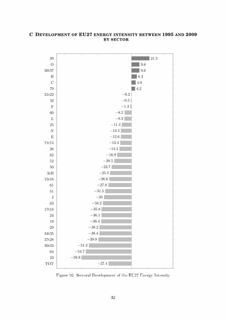
C DEVELOPMENT OF EU27 ENERGY INTENSITY BETWEEN 1995 AND 2009BY SECTOR

−80 −60 −40 −20 0 20 40

TOT

23

64

30t33

27t28

34t35

29

19

24

17t18

63

J

51

61

15t16

AtB

50

52

62

26

71t74

E

N

25

L

60

F

M

21t22

70

C

H

36t37

O

20

−27.4

−59.9

−54.7

−51.2

−39.9

−38.4

−38.2

−36.4

−36.1

−35.8

−34.2

−33

−31.5

−27.8

−26.6

−25.5

−23.7

−20.5

−16.9

−14.4

−13.4

−12.6

−12.5

−11.4

−8.3

−8.2

−1.3

−0.5

−0.2

4.2

4.9

6.3

9.6

9.6

21.5

Change in Energy Intensity in % from 1995 to 2009

1

Figure 10: Sectoral Development of the EU27 Energy Intensity

32

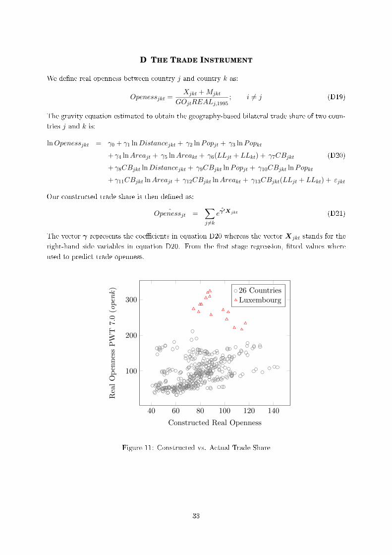
D THE TRADE INSTRUMENT

We de�ne real openness between country j and country k as:

Openessjkt =Xjkt +Mjkt

GOjtREALj,1995; i 6= j (D19)

The gravity equation estimated to obtain the geography-based bilateral trade share of two coun-

tries j and k is:

lnOpenessjkt = γ0 + γ1 lnDistancejkt + γ2 lnPopjt + γ3 lnPopkt

+ γ4 lnAreajt + γ5 lnAreakt + γ6(LLjt + LLkt) + γ7CBjkt (D20)

+ γ8CBjkt lnDistancejkt + γ9CBjkt lnPopjt + γ10CBjkt lnPopkt

+ γ11CBjkt lnAreajt + γ12CBjkt lnAreakt + γ13CBjkt(LLjt + LLkt) + εjkt

Our constructed trade share is then de�ned as:

ˆOpenessjt =∑j 6=k

eγ̂′Xjkt (D21)

The vector γ represents the coe�cients in equation D20 whereas the vector Xjkt stands for the

right-hand side variables in equation D20. From the �rst stage regression, �tted values where

used to predict trade openness.

40 60 80 100 120 140

100

200

300

Constructed Real Openness

RealOpen

nessPW

T7.0(openk) 26 Countries

Luxembourg

1

Figure 11: Constructed vs. Actual Trade Share

33

Dependent Variable: OLS Estimates

log Openness Coe�cients t-Statistic

log_ Distance -0.943*** -58.10

(0.016)

log_ Pop_ j -0.069*** -5.30

(0.013)

log_Area_ j 0.043*** 0.04

(0.011)

log_ Pop_ k 0.531*** 40.25

(0.013)

log_Area_ k -0.003 -0.34

(0.010)

CommonLandlocked -0.158*** -5.69

(0.028)

CB 0.573 1.42

(0.403)

CB_ Dist -0.359*** -3.06

(0.117)

CB_ Pop_ j -0.472*** -8.94

(0.053)

CB_ Area_j 0.612*** 11.49

(0.053)

CB_ Pop_k 0.194*** 4.14

(0.047)

CB_ Area_k -0.223*** -4.45

(0.050)

CB_ LL 0.273*** 4.6

(0.067)

constant -2.196*** -16.654

(0.132)

Model Summary:

Observations 22224

F-Statistic 839.59

Adj. R2 0.266

Root-MSE 1.973

* p<0.10, ** p<0.05, *** p<0.01, robust standard errors appear in parentheses

Table 7: Estimation Results for Gravity Model

34

E THE INCOME INSTRUMENT

The estimation equation for the instrument of income is:

ln

(Real_GDP

Pop

)jt

= α0 + α1 ln

(Real_GDP

Pop

)jt−1

+ α2 ln

(Real_I

GDP

)jt

+α3 ln(n+ g + δ)jt + α4 lnLABHSjt + α4 lnKHcjt

+α4 ln

(K

L

)+ α4 lnRealOpennessjt + εjt (E22)

Dependent Variable: Fixed Effects Estimates

log Real GDP per Capita Coe�cients t-Statistic

ln(

Real_GDP

Pop

)jt−1

0.881*** 45.67

(0.02)

ln(

Real_I

GDP

)jt

0.140*** 7.15

(0.02)ln(n+ g + δ)jt -0.137*** -4.57

(0.03)lnLABHSjt 0.030* 1.96

(0.02)lnKHc

jt 0.186 1.68(0.11)

ln(

KL

)-0.018 -0.63

(0.03)lnRealOpennessjt 0.011 0.42

(0.03)constant 0.323* 1.76

(0.18)

Model Summary:Observations 375F-Statistic 1332.95Adj. R2 0.9797

* p<0.10, ** p<0.05, *** p<0.01, robust standard errors appear in parentheses

Table 8: Estimation Results for Income Instrument

F COMPARISON OF OUR RESULTS TO METCALF (2008)

In this section we compare our results to the ones in Metcalf (2008). We reported �xed-e�ects

panel estimations using the obtained index values as the dependent variables.

35

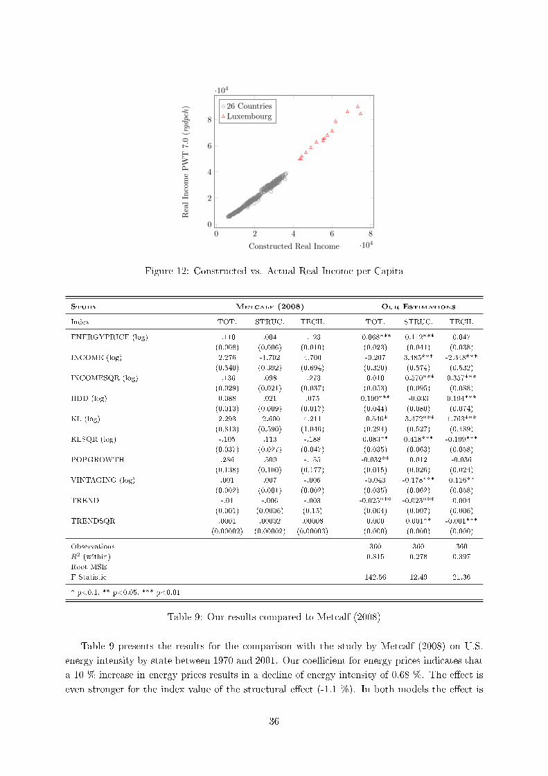
0 2 4 6 8

·104

0

2

4

6

8

·104

Constructed Real Income

RealIncomePW

T7.0

(rgdpch) 26 Countries

Luxembourg

1

Figure 12: Constructed vs. Actual Real Income per Capita

Study Metcalf (2008) Our Estimations

Index TOT. STRUC. TECH. TOT. STRUC. TECH.

ENERGYPRICE (log) -.110 .004 -.123 -0.068*** -0.112*** 0.047

(0.008) (0.006) (0.010) (0.023) (0.041) (0.038)

INCOME (log) 2.276 -1.702 4.700 -0.207 3.485*** -2.348***

(0.540) (0.392) (0.694) (0.320) (0.574) (0.532)

INCOMESQR (log) -.136 .098 -.273 0.010 -0.570*** 0.357***

(0.029) (0.021) (0.037) (0.053) (0.095) (0.088)

HDD (log) 0.088 .021 .075 0.190*** -0.033 0.194***

(0.013) (0.009) (0.017) (0.044) (0.080) (0.074)

KL (log) 2.293 -2.600 4.211 -0.546* -3.472*** 1.763***

(0.813) (0.590) (1.046) (0.294) (0.527) (0.489)

KLSQR (log) -.105 .113 -.188 0.083** 0.418*** -0.199***

(0.037) (0.027) (0.047) (0.035) (0.063) (0.058)

POPGROWTH .286 .500 -.155 -0.032** 0.012 -0.036

(0.138) (0.100) (0.177) (0.015) (0.026) (0.024)

VINTAGING (log) .001 .007 -.006 -0.043 -0.178*** 0.116**

(0.002) (0.001) (0.002) (0.035) (0.062) (0.058)

TREND -.01 -.006 -.003 -0.025*** -0.023*** 0.004

(0.001) (0.0006) (0.15) (0.004) (0.007) (0.006)

TRENDSQR .0001 .00002 .00008 0.000 0.001** -0.001***

(0.00002) (0.00002) (0.00003) (0.000) (0.000) (0.000)

Observations 360 360 360

R2 (within) 0.815 0.278 0.397

Root MSE

F-Statistic 142.56 12.49 21.36

* p<0.1, ** p<0.05, *** p<0.01

Table 9: Our results compared to Metcalf (2008)

Table 9 presents the results for the comparison with the study by Metcalf (2008) on U.S.

energy intensity by state between 1970 and 2001. Our coe�cient for energy prices indicates that

a 10 % increase in energy prices results in a decline of energy intensity of 0.68 %. The e�ect is

even stronger for the index value of the structural e�ect (-1.1 %). In both models the e�ect is

36

statistically signi�cant (p < 0.01). Surprisingly, the index value for the technology e�ect is not

a�ected by the energy price. In contrast to Metcalf (2008), income (and its squared term) has

no impact on the total e�ect. This is mainly due to the shorter time-period under investigation.

Yet when we hold technology constant, the e�ect of INCOME and INCOMESQR supports an

increasing, but inverted, u-shape relation between income and energy intensity. The calculated

turning point - when an increase in INCOME leads to an increase in energy intensity - is ≈21,200 US-$ (1995). This is exactly the median of the INCOME in our sample. In other words,

an increase in income leads to a decrease in energy intensity in half of the sample, provided

technology holds constant. Countries with more heating degree days have, ceteris paribus, a

higher index value for energy intensity. The magnitude is larger than in Metcalf's study. The

most signi�cant di�erences in our estimates are the coe�cients for the capital-to-labor ratios. An

increase in the capital-to-labor ratio leads to a decrease in the total e�ect and in the structural

e�ect. The turning point for the total e�ect is a capital-to-labor ratio of 26.3, or around the 15 %

percentile in the distribution of the sample's capital-to-labor ratios. The corresponding turning

point for the structural e�ect - again, holding technology constant - is 63.8 (around the 30 %

percentile). The estimate for POPGROWTH is negative and signi�cant on the 5 %-level for

the total e�ect index. Hence, fast growing countries have lower energy intensities. The capital

vintaging e�ect is only observable in the regressions of the structural index. There, countries

with higher investment-to-gross-output ratios tend to have lower energy intensity. The time

trend variables are negative and signi�cant in the models that explain the total e�ect and the

structural e�ect.

37