TRANSPORTATION RESEARCH RECORD 1298

Peak-Load-Congestion Pricing of Hub Airport Operations with Endogenous Scheduling and Traffic-Flow Adjustments at Minneapolis-St. Paul Airport

JOSEPH DANIEL

Hub airlines schedule banks of flights that create periodic demand peaks. During these peaks, arrival and departure rates approach or exceed airport capacity and queues develop. Under the current weight-based landing-fee structure, excessive delays result be­cause airlines ignore the delays their operations impose on other airlines and their passengers . Congestion-based airport pricing would encourage airlines to use larger aircraft with lower service frequency and to shift their operations away from the peak, thereby reducing congestion. A model is presented of the adjustment of flight schedules and traffic flows in response to weight-based and congestion-based fee structures. With data from the Minneapolis­St. Paul airport , the model is applied to calculate equilibrium congestion fees, schedule frequencies, traffic patterns, landing and takeoff costs, airport revenues, and resource savings from peak-load-congestion fees.

Most major airports in the United States assess landing fees that are proportional to aircraft weight and independent of time of operation . The social cost of a landing or takeoff, however, consists primarily of the additional delay the op­eration imposes on all the aircraft and travelers using the airport at approximately the same time. These costs are es­sentially independent of aircraft weight and vary considerably with time of operation. Weight-based fees encourage frequent service by small aircraft during peak periods and fail to ap­propriately manage demand. Use of weight-based fees has led to unnecessarily high levels of congestion and delay .

FAA estimates.that airport congestion delay costs the air­lines and their passengers $5 billion annually in increased operating costs and travel time. A Transportation Research Board report (J) indicates that 21 large hub airports each experience more than 20,000 plane-hours of flight delay an­nually and predicts that within the next decade 39 airports will exceed that level. Delays at Chicago, Atlanta, and Denver could approach 100,000 plane-hours annually. Air traffic is expected to double by early in the next century. In the past, the congestion problem has been addressed mainly by in­creasing capacity. Little effort has been made to manage de­mand. Expansion of an existing airport or construction of a new airport, however, can cost several billion dollars. Given the high cost of increasing capacity, it would seem wise to make efficient use of airports before resorting to expansions or new airport construction.

Department of Economics, University of Minnesota, 1035 Manage­ment and Economics, 271 19th Avenue South , Minneapolis, Minn. 55455.

Economists have a standard solution to the congestion problem-use the price system to allocate scarce airport ca­pacity and bring demand into line with short-term supply . The optimal fee equals the marginal external delay costs that an airplane imposes on other airplanes and travelers using the airport at approximately the same time. Such fees would cause the airlines to internalize the congestion externality they cre­ate, thereby encouraging cost-minimizing scheduling deci­sions. It has been shown that if airport capacity exhibits con­stant returns to scale, congestion fees will yield revenues exactly sufficient to pay for optimal long-run capacity (2).

The role of atomistic hub-and-spoke route networks (ones in which each route is served by a different airline) is examined as the cause of traffic peaks that exacerbate the congestion problem. Existing models of traffic flows in the transportation economics literature generally assume that the traffic is at­omistically operated-each car on the highway is owned and operated independently of other cars. Previous models of airport congestion also implicitly make this assumption (3-6). This paper continues in that tradition by modeling an airport serving an atomistic hub network. The model has his­torical relevance; the Civil Aeronautics Board prevented sin­gle airlines from dominating prederegulation hub airports. In the postderegulation environment, however, many airports are dominated by a single airline that accounts for more than half the airport's operations. In scheduling airport arrivals and departures, a profit-maximizing dominant airline would internalize the delay that one of its aircraft imposes on an­other. An atomistic airline, on the other hand, would take delay as parametric. Dominant airline operations, therefore, impose less external congestion than atomistic airline oper­ations. If a constrained-optimal fee structure is not to dis­criminate between dominant and atomistic airlines, it must be a compromise between a fee equal to the external conges­tion imposed by the dominant airline and a fee equal to the external congestion imposed by atomistic airlines. The model presented here is a preliminary step toward modeling the more difficult and realistic case of an airport with a dominant hub airline and an atomistic fringe.

The model of atomistic hub scheduling (an adaptation of Mohring's (7) model of direct-service bus scheduling to an air-service network] is integrated with a model of traffic flows through an airport bottleneck. [The bottleneck model draws on the work of Vickrey (8).] In the scheduling model, the

2

airlines choose plane size and service frequency to minimize the sum of their own and their passengers' costs. In the bot­tleneck model , each airline chooses its flight's arrival time at the airport to minimize the sum of its queuing costs and lay­over costs. Traffic patterns at the bottleneck are determined endogenously. Previous congestion-based pricing models either treat traffic patterns as exogenous or assume zero intertem­poral cross-elasticity of demand (i.e ., demand is a function of the current period's price alone, and no shifting of demand to other periods occurs). The scheduling model captures the effects of intertemporal demand shifts and predicts changes in aircraft . i7.e and chedule frequency in response to conge -tion fee . The bottleneck model captures the effects of pcak­spreading in response to the fees. Together, the models enable calculation of equilibrium fees and traffic patterns. Finally, the models introduce layover delay into the analysis of airport congestion and show that the hub airlines face a trade-off between congestion and layover delays. Gains from reduced congestion are partially offset by increased layover delays for the hub airline and its passengers.

The model is applied to traffic data from the tower logs of Minneapolis-St. Paul (MSP) airport. The data set gives the time of every operation at the airport during the first week of May 1990. Because no reliable data on actual queue lengths exist, a queuing model is used to infer the expected queue lengths given the actual arrival rates . A discrete time version of a bottleneck model is then fit to the arrival and queuing data. The model estimates the equilibrium conge ·tion fees, traffic patterns, queuing delays, layover costs, airport's rev­enues, real resource savings from reduced congestion, and changes in the airlines' schedule frequency and aircraft size.

ECONOMICS OF HUB-AND-SPOKE NETWORKS

Airlines face significant economies of scale and scope in pro­viding their services . The fundament:il sr.:ile economy arises at the conveyance level. The cost of an airplane anti its crew increases less than proportionately with increases in plane size, so cost per seat-mile decreases as the number of seats on a plane increases. Economies of scope result from joint production of trips between many different city pairs. Hub­and-spoke route ne tworks enable airlines to fly passengers witb the same origin but different destinations on a single flight to the hub. Similarly, passengers with the same desti­nation but different origins can be combined on a single flight from the hub. Because a given number of passengers can be served more frequently with fewer flights on larger planes, the cost to an airline of conveying each passenger in a hub­and-spoke network is less than that by direct service. This reduction in cost is partially offset, however, by the increased circuity of routes and by the introduction of layover delay.

Airline passengers play both a consuming and a producing role in air travel. They combine airline services with their own time inputs to produce trips . The passengers' time inputs con­sist of time in transit and schedule, congestion, and layover delay. (Time in transit is the time passengers actually spend on the plane, exclusive of the time spent because of congestion delay. Schedule delay is the difference in time between the passengers' preferred departure time and the closest sched-

TRANSPORTATION RESEARCH RECORD 1298

uled departure time. Congestion delay is the time spent sitting at the gate or on the taxiway waiting for clea rance to take off plu the time spent circling in the ai r waiting for clearance t land. Layover de lay is the time that connecting pa, sengers spend at a hub airport between their first flight 's arrival and their second flight · departure. )

The passengers' time inputs required to complete a trip depend on tile rate at which the ai rline provid its services. If the airline increases its schedule frequency it · pas engers' schedul delay decrea ·e, on average , but its co t per eat increa es on the ·mailer air planes. Similarly if the airlines schedule more frequent landings a11d lakt::offs at the hub , the average layover delay will decrease but the average congestion delay will increa e. The full co l of a flight is the sum of the pas engers' time costs and the airline' s operating costs.

Given equal elasticities of demand across groups of pas­st::ngers with different time values, a profit-maximizing airline will choose the socially optimal service frequency-that which minimizes the sum of its own and its passengers' costs. An intuitive explanation of this fact is as follows. Suppose that, by increasing its service frequency , the airline could reduce its passengers' costs by more than the increase in its own costs. Then a simultaneous increase in frequency and price by an amount equal to the reduction in its passengers' costs would not change the full cost of service to passengers and, hence, the rate at which they travel. The simultaneous change in frequency and price, therefore, would increase its profits. The airline's profit-maximizing scheduling departs from socially optimal scheduling, however, insofar as uncompensated congestion externalities are imposed on other airlines and their passengers .

If the airport had unlimited capacity and flights were always on schedule, airlines would schedule all their planes to arrive at the hub airport at the same instant. There would be a brief interchange period while passengers transferred to their con­necting flights. All planes would then depart at the same instant. Unfortunately, flights deviate randomly from their expected arrival times, and airport can accommodate only a limited number of landings or takeoffs in a given period of time. As the volume of traffic increases, landing and takeoff queues develop . If the airlines scheduled all flights to arrive precisely at the beginning of the intercliange period , the flights that arrived close to their ched uled time would face long delay$ because of the high traffic volume near the beginning of tbe interchange. Some of the flights would arrive early and experience small queues but have to wait longer until the interchange period began. Others would arrive after the in­terchange began and these passengers would either delay or miss their connections. Each airline has an incentive to adjust its flight's arrival chedule to minimize the sum of its expected costs of arriving early , waiting in the queue, and arriving late . An equilibrium traffic flow results when the arrival schedules and expected queue lengths are such that no airline can reduce its flight's expected co ts by changing its schedule. Assuming that all aircraft have identical co ts, the equilibrium expected cost of scheduling an arrival at all periods must be identical­otherwise, flights scheduled at high-cost periods could reduce costs by moving to low-cost periods. These observations about airline scheduling will be formalized in a model in the next two sections.

Daniel

MODEL OF ATOMISTIC HUB-AND-SPOKE ROUTE NETWORK SCHEDULING

Atomistic airlines operate a hub-and-spoke route network that serves a large hub city located at the center of a circular market and n rim cities located at equal intervals around the circle's circumference. It takes h hours to fly from hub to rim. The cost per hour of flying an airplane with P passengers is aPb, where a and b are cost parameters . A bank of 2*n flights can convey travelers between all cities in the route network. The cost to the network of flying all the airplanes in one bank from the rim cities to the hub and back again is $2naPbh.

Travelers in each direction on hub-to-rim (or rim-to-hub) and rim-to-rim routes have desired departure times that are uniformly distributed at the rate of Dh and D, per hour, re­spectively . Random variations in demand are ignored. On each airplane, the hub combines passengers on a hub-to-rim (or rim-to-hub) route with passengers on (n - 1) rim-to-rim routes. The effective demand density for each flight in a bank is therefore D = Dh + D, (n - 1) travelers per hour. If the airplanes all have P passengers , there will be DIP banks per hour and the interval between banks will be PID hours . On average, a passenger will experience a schedule delay equal to 1/cx of the interval between banks, where 1/a is in the interval Y4::; 1/cx ::; Y2. If all passengers choose the flight closest to their desired departure time, then l/cx = Y4, and if all passengers pick the flight that will arrive at a destination before a given time, then l/cx = Y2. Let r = D,(n - 1)/D be the fraction of indirect passengers on each flight. In each bank there are nP passengers originating at the rim cities and (1 - r)nP passengers originating at the hub. If the average passengers pays $v0 per hour to avoid schedule delay, then the total cost of all passengers' schedule delay is [(2 - r)nPv0 ]PI (cxD) per bank.

There are rnP indirect passengers in each bank who have to spend 2h hours in transit and 2(1 - r)nP direct passengers in each bank who spend only h hours in transit . If the average passenger pays $v1 per hour to shorten the length of a trip, then the total cost of all passengers' time in transit is 2nPhv 1

per bank. The airlines and their passengers also experience costs caused

by congestion and layovers at the hub airport. Let C" and Cd denote the sum of congestion and layover costs experienced by an airplane and its passengers on landing at and taking off from the hub airport. Let C; denote the cost of time spent during the interchange period. c. and Cd are determined be­low in the bottleneck model and C; is a parameter. The total cost of congestion and layover is n( C0 + Cd + C;).

The sum of the passengers' and airlines' cost of operating the hub-and-spoke network for an hour is

D p p {2naPbh + [(2 - r)nPv0 ] aD

+ 2nPhv1 + n(C0 + Cd + C;)} (1)

A profit-maximizing or full-cost-minimizing hub network would choose P to minimize expression 1.

To simplify the previous scheduling problem, all the rim cities in the hub-and-spoke network are assumed to be equi-

3

distant from the hub, and all have identical demand densities. As a result, the optimal plane sizes and service frequencies are identical for all the hub's routes . This· greatly simplifies the mathematics of the model. In reality, however, the airline faces different demand densities and different flight distances, so its bank interval cannot simultaneously optimize service on each route. Some cities with low demand density may not be served in every bank. Increasing airport fees may cause some cities to be served in fewer banks, resulting in lower congestion and higher schedule delay. The model does not capture this effect and therefore tends to underestimate the reduction in congestion costs that would result from conges­tion pricing.

DISCRETE TIME BOTTLENECK MODEL WITH STOCHASTIC ARRIVALS

Let S, denote the number of flights scheduled to arrive during period t and p1 the probability that a flight will arrive j periods from its scheduled time. If A, denotes the expected number of arrivals during period t, then

Let Q, = Q(Q,_ 1, A,_ 1) denote the expected length of the queue at the beginning of period t, a function of the expected queue at the beginning of the previous period and the ex­pected number of arrivals during the previous period. Let k be the number of airport operations that can be performed in one period. The expected delay, D,, experienced by planes arriving in period tis D, = (Q, + Q,+1)/(2k). Let Cq be the amount that an airline and its passengers would be willing to pay to avoid one period of queuing delay . Similarly, let c. and C1 be the amount that they would be willing to pay to avoid a period of earliness or lateness . The beginning of the interchange period occurs at period T0• The expected cost of a landing scheduled for period t is

C, = Cq L p1 D,+1 + C. L pJTo - (t + j J Js. To - r-Dr +;

+ D,+)] + C, L pJ(t + j + D,+) - T0 ] j > To-r-Dr+ j

A no-fee atomistic bottleneck equilibrium is a sequence {S,, A,, Q,, D,, C,}, T = ( - oo . .. oo), that, given p , Cq , C., C" k , and a queuing process , Q (-) , satisfies

D, = (Q, + Q,+ 1)1(2k)

C, = Cq L p1D,+1 I

+ C. L p1 [To - (t + j + D,+) ] j s.To- 1-D1+j

+ C, L p1 [(t + j + D,+) - To] j > TO - t-D1+j

(2a)

(2b)

(2c)

(2d)

4

and

(S, > 0) ~ (C, ~ C,.) for all t and t' (2e)

The optimal congestion fee, F,, is equal to the marginal external congestion imposed by a landing in period t. Define the sequence A' such that A; =A; for i<>t and A; = A; + r for i = t. Define the sequence Q' such that Q; = Q(Q;_ 1 ,

A;_ 1) and the sequence D' such that D; = (Q; + Q;+ 1)/(2k). The delay cost incurred by a flight that actually arrives at period tis

and

Define the sequence C' such that

and

Now the optimal congestion fee can be written as

F, - L (A;C; - A;C;)IE t 5 i

A congestion-fee atomistic bottleneck equilibrium is a se­quence {S,, A,, Q,, D,, C,}, t = ( - oo . .. oo), that, given p, Cq, C., Cl> k, and Q(·) , satisfies Equations 2a, 2b, 2c, 2e, and

C, = c . 2,p;D,+; + C0 2, pJT0 - (t + j + D, ,;)] I j :s. Tn -t-Dr+j

+ C, 2, P; [(t + j + D, +;) - T0] + LP;F1 +; (2d') j> TO-t - Dr +j j

Identical equilibriums can be defined for takeoff schedules, exce.pt that p, Cq, C., C1, k, and Q(·) may take different values . There is much less randomness in the departure than the arrival process, sop has a different distribution . Similarly, cq changes because the cost of being in the takeoff queue is lower than that of being in the landing queue. The relative values of Ce and C, in the takeoff schedule problem are the reverse of those in the landing problem. As stated previously, the equilibrium values of the expected cost of a scheduled landing (takeoff) are identical for all tin which arrivals (de­partures) are scheduled. The equilibrium values of C, for ar­rivals antl departures are the c. and Cd that appear in the scheduling model.

Two assumptions made previously greatly simplify the bot­tleneck model-that all flights have identical cost parameters, Cq, C., and C1, and that all flights are part of the hub route network with the same desired arrival and departure times. As a consequence of these assumptions, the model ignores cost savings resulting from a relatively greater incentive for small flights and nonhub flights to shift their arrival and de­parture times away from the peaks. More will be said about

TRANSPORTA TI ON RESEA RCH RECORD 1298

this point subsequently. Much of a typical airport's traffic , however, is part of its hub network. Code-sharing airlines cooperate with the dominant hub airline in scheduling and marketing their flights-they clearly are part of the network . Some unaffiliated regional-carrier flights and general-aviation flights transfer passengers to the hub flights: they, too, prefer to operate close to the hub's interchange period. Although nonhub commercial carriers do nol carry many passengers who want to make interline transfers , these flights are often scheduled for times close to the hub's flights to match the hub's service times and because the hub's banks occur at popular times of the day for travel. The nonhub carriers must have a substantial preference for operating at the same time as the hub's bank, because they are willing to incur the sub­stantial delays associated with it. Assuming that they prefer to land at the interchange times exaggerates the costs of shift­ing these flights off the peak and tends to underestimate the benefits of congestion pricing but is probably not too un­realistic.

DATA AND EMPIRICAL SPECIFICATION OF THE MODEL

To implement the model requires estimation of Q(-), p, Cq, C., C1, and k . Landing and takeoff data were gathered from the tower logs of MSP airport for all operations on May 1, 2, 3, 4, and 8, 1990. The data show the flight number, aircraft type, destination (if a departure), and time that the aircraft contacted the tower to join the landing or takeoff queues. Figure 1 shows the average number of arrivals and departures that occurred during each 10-min interval on those days. The different shading of the bars indicates how many of the op­erations were attributable to Northwest Airlines (NWA); its code-affiliates, Express (NWX) and Mesaba (MES); other national carriers (OTH); general-aviation (GA); or air freight, military, and independent regionals (MISC) . The importance of Northwest Airlines' (i .e., the hub's) banks in creating the peak demand periods is evident from the graphs. It is also clear, as discussed earlier, that large numbers of other aircraft are willing to incur delays and operate during the bank pe­riods. This implies that their preferred schedule time is during the bank. The double vertical lines indicate the scheduled interchange periods, which are generally 30 min long. An interesting feature is that many departures overlap the sub­sequent bank's arrivals, even when minor adjustments would seem to avoid the overlap. This suggests that a mix of landings and takeoffs may require little more time than would be re­quired for the landings alone . Note also that arrival peaks are lower and less steep than departure peaks-a fact attributable to the greater randomness in the arrival process.

Table 1 summarizes the peak demand periods at MSP. Northwest operates nine banks of arrivals and departures in about 17 hr each day . The average interval between banks is approximately 1.9 hr. Northwest's banks alternate service be­tween east-to-west routes and west-to-east routes, so that a given route in a given direction is generally served on every other bank. The highest-density routes, however, may be served in each direction on virtually every bank, whereas the lowest­density routes may be served only once a day . The largest banks interchange passengers between nearly every city in the

Daniel

Flights per Interval

14

12

10

AclUUI A(J lv81$ OS· 15 Actual Arrivals 15-24

.NWA

[I twX

• tvES

• OTH

II GA

5

06 06 06 07 07 07 08 08 08 09 09 09 1 0 , 0 1 0 11 11 11 12 12 12 13 13 13 14 14 , 4 15 15 15 16 1 6 16 17 1 7 17 1 8 1 8 18 19 19 19 20 20 20 21 21 21 22 22 22 23 23 23 24 00 20 40 00 20 40 00 20 40 00 20 40 00 20 40 00 20 40 00 20 40 00 20 40 00 20 40 00 20 40 00 20 40 00 20 40 00 20 40 00 20 40 00 20 40 00 20 40 00 20 40 00 20 40 00

Flights per Interval

1 e

16

14

12

10

Aclual Departures 06-15 Actual Deparlures 15-24

· J~~1 m i liJJ . L 1 dt1 II~~ Ji.~ 1J l 1]~J~tllt _, 06 06 06 07 07 07 OB 08 00 09 09 09 1 o 1 o 1 O 11 11 11 12 12 12 13 13 13 14 14 14 15 1 S 15 16 16 16 17 17 17 18 18 18 19 19 19 20 20 20 21 21 21 22 22 22 23 23 23 24 00 20 40 00 20 40 00 20 40 00 20 40 00 20 40 00 20 40 00 20 40 00 20 40 00 20 40 00 20 40 00 20 40 00 20 40 00 20 40 00 20 40 00 20 40 00 20 40 00 20 40 00 20 40 00

FIGURE 1 Arrivals and departures by 10-min intervals.

hub-and-spoke network, whereas the small banks serve only Previous studies of airport queues have assumed a single queue the denser routes. operated on a first-come, first-served basis with no distinction

Unfortunately, no reliable data exist about the lengths of between landings and takeoffs. It is more convenient here to the landing and takeoff queues. It is necessary, therefore, to assume a polar-opposite queuing discipline-two indepen-use a queuing model to infer the lengths of the queues given dent queues, each operated on a first-come, first-served basis airport capacity, the arrival and departure process, and sev- with no interaction between landings and takeoffs. The truth era! simplifying assumptions about the queuing discipline. probably lies somewhere between these poles. Using hourly

TABLE 1 TIMING AND SIZE OF FLIGHT BANKS AT MSP

Time Type NWA NWX MES am GA MISC TOTAL

06:00-07:00 Arrivals 1 5 7 8 4 7 0 41 07:40-08:30 Departures 28 7 6 I 1 9 I 62 07:30-08:40 Arrivals 27 6 2 4 1 0 I 50 09:00-09:20 Departures 26 5 6 4 7 0 48 09 :40-11 :00 Arrivals 28 8 5 1 1 7 3 62 11 :30-12:00 Departures 26 6 2 7 4 0 45 11 :40-12:20 Arrivals 29 4 6 9 9 0 57 12:50-13:30 Departures 33 6 9 6 3 0 57 13:00-14:00 Arrivals 20 7 2 1 2 4 0 45 14:30-15:00 Departures 1 9 6 2 7 2 0 36 16:00-17:20 Arrivals 34 7 9 1 5 1 6 2 83 17:40-18:20 Departures 30 9 7 9 4 I 60 17:40-18:40 Arrivals 32 6 5 4 9 3 59 19:20-19:40 Departures 30 2 5 3 1 0 4 I 19:00-20:10 Arrivals 1 7 2 2 9 1 0 8 48 20:30-21:10 Departures 1 9 4 3 3 3 1 33 20:20-22:00 Arrivals 28 4 5 1 0 6 9 62 22:30-22:50 Departures 1 2 5 3 2 4 27

6

20

10

0

g II

• • • • • • • • • • • • • • • II

••••• • D •• •

• • • II

• • II •

• II • • II ••

II • • • 11

10 20

FIGURE 2 Landing and takeoff capacity for 10-min intervals.

arrival, departure, and delay data, Morrison and Winston (9) found that landings have about twice the effect of takeoffs on delays experienced by an arriving airplane. Similarly, takeoffs have about twice the effect of landings on delays experienced by a departing airplane. Figure 2 shows the number of land­ings and takeoffs performed at MSP during 10-min intervals on the afternoon of April 24, 1990. The graph of the landing and takeoff possibilities frontier indicates some interdepen­dence between landing and takeoffs, but it is not linear as implied by the single-queue model. In the absence of adequate data to calibrate a more complicated queuing model, the as­sumption of two independent queues is adopted.

Arrivals and departures are assumed to be Poisson distrib­uted, with time-varying Poisson parameters equal to the av­erage arrival and departure rates for each 10-min interval as given in Figure 1. The expected queue lengths are calculated for the given arrival and departure distributions using Omo­sigho and Worthington's (10) discrete time queuing model for single-server queues with inhomogeneous arrival rates and discrete service time distributions. The model uses the prob­ability distribution on queue lengths as a state vector and uses recurrence relations to calculate the state vector for each ser­vice interval given the time-varying arrival rate distributions. Because constant capacity is assumed, the model is similar to a Markov transition model, with the probability distribution on queue sizes as the state and transition matrices for each service interval, which change every 10 min to reflect the current distribution of arrivals. The calculations are based on an assumed airport capacity, k, of nine landings and nine takeoffs per 10-min interval.

Figure 3 shows the arrival and departure rates and the resulting expected queue lengths at the beginning of each 10-min interval. The arrival banks tend to peak and plateau at between 10 and 12 arrivals per 10-min interval. Arrival queues develop only during the hub banks and return to nearly zero as the bank ends. Their peaks do not plateau, and range in height from about 4 to 10 aircraft, depending on the size of the bank. The arrival rates and queue sizes increase and decrease at roughly the same rates across banks with different

TRA NSPORTATION RESEARCH RECORD 1298

numbers of flights. The departure rates and queue sizes are relatively more highly peaked, and increase and decrease more quickly. The rates of departure peak at between 10 and 18 flights per interval, and the queue sizes achieve similar mag­nitude. Departure queues are significant only during the hub banks.

Although the queuing model is necessary for initial esti­mation of expected q11e11e lengths, it is too computation<illy cumbersome to use in the bottleneck model. A regression model, however, can be fit to the queue estimates and the arrival and departure data . The regression equation is

The regression estimates (with t-values in parentheses) are

QI= -0.046 + 0.07QI-) + 0.021A/-l + 0.045Q/-I A t-I (-1.012) (4.093) (1.363) (33.739)

+ 0.027Q~_ 1 + 0.028A~_ 1 Rz .995 (26.384) (23 .676)

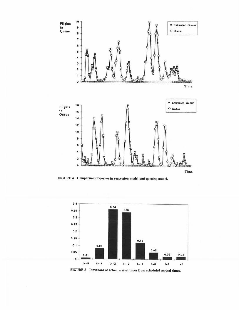
Figure 4 compares the evolution of the queuing systems as estimated by the queuing model and the regression model. The simple regression model appears to describe the evolution of the queues remarkably well.

To estimate the probabilities that tht: actual arrival anti departure times deviate from the scheduled time by j periods (i.e., p;), the actual arrival and departure times reported in the tower log were matched with the flights' scheduled times reported in the Official Airline Guide (11). The p1 histogram for arrivals is shown in Figure 5. The histogram indicates the probability that a flight scheduled to arrive at the gate at period t = 0 actually arrives at the queue during periods t = - 5 to 2, where each period is 10 min long. For example, 5 percent of all flights arrive at the landing queue during the 10-min interval centered on the time they arc scheduled to arrive at the gate. On average, flights arrive at the queue 1 R min before their scheduled arrival time at the gate, to allow ample time to land and taxi to the gate. For departing flights, 97 percent of the times reported in the tower logs were within the same 10-min interval as their scheduled departme times. The tower log reports a few deviations from scheduled de­parture times, but no other time interval accounted for as much as 1 percent of the deviations. Frequent fliers will be excused for suspecting that the logs do not tell the whole story, but in the absence of better information, all flights are assumed to depart at their scheduled time (i .e., p 0 = 1).

The cost parameters Cq, C., and C, can be estimated from observations of expected queue lengths, expected early-time deviation, and expected late-time deviation. Manipulating the equilibrium cost equation yields

" D = C* _ C, ~ [ L.,, P; 1+; C C L.,, P; To - (t + j + D1+)]

j q q i""'To-1-D1+1

c, ~ . + c L.,, P;[(t + J + D1+) - T0]

q j > To-1-D1 +J

It follows that least squares estimates of C) Cq and C1/Cq can be obtained by regressing observations of expected delay

Daniel

Flights per 12

Interval/ Flights

10 in Queue

8

6

..

2

n

Flights per

18 Interval/ Flights 16 in

14 Queue

12

1 0

8

6

2

0

FIGURE 3 Arrivals, departures, and queue lengths.

"i,ipiD• +i on observations of expected early time

L Pi [T0 - (t + j + D,+)] js.To - 1- D1 + j

and expected late time

L Pi [(t + j + D,+;) - T0 ] j > To - t - D1 + j

Only time periods during which arrivals or departures were actually scheduled can be used in the regression. Because C* may vary for each bank, a dummy variable must be entered in the regression for each bank (except the first) from which data are used. The regression constant plus the relevant dummy coefficient can be interpreted as an estimate of C*/Cq for that bank. Using data from the six largest arrival banks, the es­timates for the arrival costs and their t-values are

Exp delay= 0.673 + 0.03782 + 0.034B3 + 0.28284 + 0.39285 + 0.51386

(6.317) (0.872) (0.81) (6.416) (9.239) (10.831)

+ 0.134 (exp early time) + 0.932 (exp late time) (5 .405) (1.112) R' = .961

Arrivals & Queues

Depanures & Queues

• Queues

D Arrivals

T ime

•Queues

[] Departures

u

Time

7

Because actual departure periods deviate practically not at all from scheduled departure periods and there are virtually no departures during the interchange periods, expected early time is omitted in the departure cost regression, and the early­time cost is assumed to be sufficiently large that no flights are scheduled to depart during the interchange. Using data from the seven largest departure banks, the estimates for the de­parture costs are

Exp delay= 0.826 + 0.11482 - 0.28483 + 0.30884 - 0.72485 + 0.00886

(5.425) (0.695) ( -1.731) (1.874) ( -4.311) (0.051)

- 0.13187 + 0.169 (exp late time) R2 = .868

(-0.8) (3.737)

The high R2s in the regressions suggest that the airlines do trade off expected queuing delays against expected early and late times in accordance with the model.

Although the bottleneck model depends only on the ratios C)Cq and C/Cq, the scheduling model requires assigning some monetary values to the parameters. Suppose that 10 min of queuing delay on landing costs the airlines and their passen­gers $350 per flight. Because early time on arrival is identical

Flighls 10

~ E•Um•"' a"'J in 9 Queue D Queue

8

7

6

5

4

0 3

2

0

Time

• Estimated Queue

Flighls 18

in 16 Queue

14

12

10

8

6

4

2

Time

FIGURE 4 Comparison of queues in regression model and queuing model.

0.36

0.05

- 0 .02

lllllllL.r-- -'. 0 .02

1··5 l·-4 l·-3 1--2 1--1 1-0

FIGURE 5 Deviations of actual arrival times from scheduled arrival times.

Daniel

to late time on departure, it follows that Cq = 350, Ce = 46.9, and C1 = 326.2 on arrival and that Cq = 277.5 and C1

= 46.9 on departure. Having estimated a queuing process, Q( ·), the probabili­

ties, pi, and the cost parameters, Cq, C,, and C1, the equilib­rium S, A, Q, D, C, and F can be determined. The solution technique takes an initial sequence, S, and iteratively moves incrementally smaller numbers of scheduled arrivals from the highest-cost period to the lowest-cost period. After each iteration's change in S, the sequences A, Q, D, F, and Care recalculated. The algorithm quits when the expected cost of a landing (takeoff) in any period during which flights are scheduled converges to within 0.1 percent of all other such periods' costs. The system converges to the same equilibrium from widely differing initial sequences.

RESULTS

Figure 6 compares the equilibrium arrival and departure rates in the no-fee and congestion-fee equilibriums for hypothetical

9

banks of 40, 45, 50, 55, and 60 flights. The hypothetical no­fee arrival banks look quite similar to their similar-sized coun­terparts in Figure 3. In both, the banks begin to plateau at about 10 operations per 10 min, with larger banks spreading operations away from the interchange periods. As expected, the congestion-fee equilibrium arrival banks are more spread out than the no-fee banks. Their arrival rates peak more slowly and reach only 80 percent as high.

As with the departure banks of Figure 3, the hypothetical no-fee departure banks of Figure 6 have much steeper and higher peaks than their corresponding arrival banks. In con­trast to Figure 3, however, they are much higher and oscillate between high departure rates and no departures. In the ab­sence of a fee, many flights attempt to leave immediately after the interchange period. A large queue develops, and no new flights join the departure queue until it diminishes. When the queue is short enough, there is another rush to leave and the process is repeated. These oscillations appear to dampen as the number of flights in a bank increases. The hypothetical congestion-fee banks, on the other hand, have quite modest

Comparison of Arrivals

• Arrivals ( No Fee )

D Arrivals ( With Fee )

Flights 12

per Interval 10 -

8

6

4

2

0

n = 40 n = 45 n = 50 n = 55

Comparison of Departures

Flights 30

per Interval 25 '

20

15

10

5

0

n = 40 n = 45 n = 50 n = 55

FIGURE 6 Effect of congestion fees on arrival and departure rates.

n = 60 Time

• Departures ( No Fee )

D Departures ( with Fee )

n = 60 Time

10 TRANSPORTATION RESEARCH RECORD 1298

• · Queues ( No Fee )

Comparison ol Queues for Arrival O Queues ( With Fees )

Fligh ts 8

in 7 Queue

5

4

3

2

0

n = 40 n = 4S n =SO n = SS n = 60 Time

Comparison ol Queues lor Departure • - Queues ( No Fee )

o Queues ( with Fee )

Flights 25

in Queue 20

15

10

5

0

n = 40 n = 4S n =SO n = 55 n = 60 Time

FIGURE 7 Effect of congestion fees on arrival and departure queue.

peak-departure rates immediately following the interchange and very even and gradual tapering off of departures.

Figure 7 shows the changes in queues that result from im­posing equilibrium congestion fees. The no-fee hypothetical arrival queues look very similar in slope and magnitude to those of Figure 3. They tend to peak with similar slopes re­gardless of bank size; larger banks have progressively higher queue peaks. Congestion-fee arrival queues are more spread out and achieve only about 50 percent of the peak size of no­fee queues. The reduction in departure queues is much more dramatic. Because of more even spreading of the congestion­fee departure rates, the departure queues are very small. The peak congestion-fee departure queue is about 17 percent as long as the corresponding no-fee queue. On average, flights experience much less queuing delay in the congestion-fee equilibrium but experience higher early- and late-time costs because of the peak-spreading. Those familiar with standard formulations of bottleneck models may wonder why any queues exist in the congestion-fee equilibrium. The standard for­mulation assumes no randomness in the arrival or departure process. Queues only develop when traffic exceeds capacity. The queuing process used here is estimated from a queuing model with Poisson arrivals and departures that generate pos-

itive queues with arrival or departure rates below capacity. Eliminating the queues would require very low arrival or departure rates and very long layover delays.

Figure 8 shows the change in marginal external congestion between the no-fee and congestion-fee equilibriums. The mar­ginal external congestion schedules in the congestion-fee cases are, of course, the equilibrium congestion-fee schedules. The peak external congestion costs caused by arrivals decrease by about 50 percent in response to the congestion fees . The peak external congestion costs caused by departures decrease by between 66 and 75 percent. The equilibrium arrival fee sched­ule increases almost linearly with time as flights approach the interchange period. It peaks just before the interchange and then decreases very quickly, almost linearly. The equilibrium departure fees peak in the period following the interchange and decrease gradually with time, almost linearly. Thus, the optimal fees can be approximated using a simple piecewise linear fee schedule.

Two additional observations should be made regarding Fig­ures 6 through 8. Randomness in the arrival process appears to mitigate the congestion externality problem. Peak external congestion levels are 50 to 66 percent less for no-fee arrival banks than for no-fee departure banks. Bottleneck models

Daniel 11

•Fee Comparison of Exlernal Congesllon and Fees for Arrival

o External Congestion

$ 700

600

500

400 ~ [

300

200

100

0 II

n = 40 n = 45 n = 50 n = 55 Time

• Fees Comparison of Exlernal Congeslion and Fees for Departures

o External Congeslion

$ 2500

2000

1500

1000

FIGURE 8 Comparison of external congestion and equilibrium fees.

that ignore randomness in the arrival or departure processes may seriously overstate the levels of congestion and the ben­efits of congestion pricing. That departures may be more ran­dom than indicated by the tower log data may explain why the departure rates and queues for the hypothetical no-fee banks are much higher and steeper than those in Figure 3. A second explanation may be that internalization of delay by the hub airline accounts for the difference . The actual rates of departure shown in Figure 3 fall between the hypothetical no-fee and the congestion-fee departure rates, as might be expected if the hub airline were partially internalizing delays.

Table 2 shows the changes in landing and takeoff costs per flight resulting from imposition o( congestion fees. Columns 2 through 5 are the equilibrium values of Ca and Cd for the no-fee and congestion-fee equilibriums, respectively. Column 5 is the sum of Ca, Cd, and the weight-based fee for an average­sized aircraft (130,000 lb). In 1990, the weight-based fee at MSP was $0.70/1,000 lb, so the average fee was $91. Column 6 is the sum of C and Cd for the congestion-fee equilibrium . Column 7 shows the increase in cost per flight resulting from the congestion fees. Depending on bank size , the increase in cost is between 60 and 95 percent of the weight-based fee and about 10 percent of total landing and takeoff costs with a weight-based fee.

Table 3 shows the changes in airport revenues and resource savings per flight bank resulting from switching to congestion pricing. Airport revenues from the fees would increase three­to four-fold. The average increase in airport revenue per flight more than offsets the additional landing and takeoff cost per flight, resulting in a resource savings per flight of $125 to $205, depending on the number of flights in the bank . These resource saving are 25 to 30 percent of the total landing and takeoff costs experienced under the weight-based fee structure.

In addition to spreading out the airport's arrival and de­parture peaks, congestion fees may also change the frequency of arrival and departure banks. The airlines choose aircraft size and flight frequency to minimize the full cost of operating the hub network as given in expression 1. To minimize expres­sion 1 requires knowledge of how Ca and Cd vary with changes in aircraft size, P, which in turn requires knowledge of how Cq, C., and C, vary with P. The cost parameters, Cq, C., and C1, are composed of passenger time costs, which are essen­tially proportional to P, and aircraft costs, which increase at approximately the 0.75 power of P. So, for example, Cq =

o.P + ~pi 75. Unfortunately, the data do not enable estimation

of the coefficients, o. and ~ , which apportion these costs be­tween passengers and airlines. Using what it is hoped are reasonable assumptions about these coefficients, the following

12 TRA NSPORTA TION RESEARCH RECORD 1298

TABLE 2 COMPARISON OF LANDING AND TAKEOFF COSTS

Landing and Takeoff Cost per

Flights in Landing Costs per Flight ($) Takeoff Costs per Flight ($) Flight ($)

Increase in Bank Weight Fee Congestion Fee Weight Fee Congestion Fee Weight Fee Congestion Fee Cost per Flight" ($)

40 282 332 314 320 45 295 360 354 353 so 322 391 391 389 55 344 418 408 416 60 363 446 444 448

"Including fees.

estimates of the relationship between landing and takeoff costs and aircraft size fit simulated data from the bottleneck model extremely well:

C., + Cd = 13.558Po·834 for the no-fee equilibrium

C0 + Cd = 13. 749Po 877 for the congestion-fee equilibrium

The weight-based fees at MSP can also be estimated as a function of P :

F = 0.24P1·23

By substituting reasonable values for the parameters m expression 1, it can be rewritten as

+ 2*60*P •2•25 + 60 [f*13.749 •Po 877 +

(1 f)~ (13 .558-tPo·834 I 0.24*P 123) I (8•P I 4•Po·75)]}

where f = 1 for congestion fees and f = 0 for weight-based fees .

These parameters are chosen so that the solution for the weight-based-fee case is P = 117 and the interval between banks is 1.9 hr-the average values for MSP. The solution for the congestion-fee case is P = 117.625, which indicates that , given this parameterization of the model, the congestion fees have virtually no effect on service intervals. An inter­esting question is whether this result would hold for networks serving markets with different demand densities . Table 2 shows that significant reductions in cost per plane would result if there were fewer planes in a bank, but serving smaller markets with lower frequency than every bank would increase schedule delay in the small market. The current model does not answer whether the cost savings from smaller banks would exceed the increase in schedule-delay costs .

TABLE 3 AIRPORT REVENUES AND RESOURCE SAVINGS

596 652 56 649 713 64 713 780 67 752 834 82 807 894 87

FURTHER RESEARCH AND CONCLUSIONS

The model suggests a number of issues for further research . Foremost among these is the need to model the internalization of congestion by a dominant hub airline. Imposing atomistic fees on it would cause it to overinternalize the delay its air­planes impose on one another , thereby spreading its arrival and departure banks out too much. Because it would be un­acceptable to have fees that favor the hub airline , the constrained-optimal single-fee structure must balance over­internalization by the hub against underinternalization by the nonhub airlines. This issue has been overlooked in the past, but it must be significant at airports where a single airline accounts for more than half of the traffic.

The model 's realism would be improved by relaxing the assumptions that all flights serve identical markets, are the same size, and have the same desired arrival and departure times at the hub. A primary political ubjecliun to imple­menting congestion pricing is its effect on service frequency in lower demand-density markets. The hub scheduling model could be extended to model networks in which some routes are served with less frequency than every bank , thereby pro­viding some insight about the effect of congestion pricing on service frequency in marginal markets.

Allowing market density to vary would also require chang­ing the bottleneck model to accommodate flights of different sizes . Different-sized flights have different queuing and layover­delay costs. In a bottleneck model with flights of different sizes, the smaller planes with lower aggregate passenger and aircraft-delay costs would shift further away from the peak. In equilibrium, similar flights would still have identical costs regardless of arrival and departure time, but flights of differ­ent sizes would have different costs. (Smaller flights generally have smaller congestion fees than larger flights because they operate at less desirable times and because they impose delay mostly on other lower-cost fli ghts .)

Finally, the model 's implications for optimal airport ca­pacity should be studied . Previous models of airport capacity have assumed that demand peaks are independent of capacity .

Avg Total Airport Revenues ($) Increase in Avg Increase in Resource Resource Gain

Flights in Airport Revenues Total Resource Gain as Percent of Bank Weight Fee Congestion Fee Revenues ($) per Plane ($) Gain ($) per Flight ($) No-Fee Costs

40 3.640 10,867 7,227 181 4,987 125 24 .7 45 4,095 13,460 9,365 208 6,485 144 25.8 50 4,550 16.647 12,097 242 8,747 175 28.l 55 5,005 19,508 14,503 264 9,993 182 27 .5 60 5,460 22,951 17,491 292 12,27 1 205 28.6

Daniel

The bottleneck model implies that additional capacity would increase the height and steepness of the demand peaks as airlines attempt to shorten the average layover period their passengers experience. Properly accounting for the benefits of additional capacity requires a model that includes layover costs and endogenous demand peaking.

Several innovations m the airport congestion-pricing liter­ature have been introduced here. An atomistic hub-and-spoke network's scheduling problem is modeled, thereby explaining the underlying causes of the periodic demand peaking ex­perienced at hub airports. The model explains how airlines choose aircraft size and service frequency to minimize full costs of service and it captures changes in service frequency in response to congestion pricing. The hub-network model also motivates the use of a bottleneck model of the timing of arrivals and departures within the network's flight banks. The bottleneck model captures peak-spreading and the important trade-off between layover and congestion delay. The standard bottleneck model is extended to allow flights to deviate ran­domly from their schedules and is given a discrete-time spec­ification that facilitates empirical application of the model. Implementing the model for MSP describes the airport's ar­rival peaks quite well but overestimates the peak rates of departure and the resulting queues and congestion. The op­timal fees have a simple structure that leads to modest in­creases in airline and passenger costs and significant increases in airport revenues and net social welfare.

ACKNOWLEDGMENTS

The author is deeply grateful to Herbert Mohring of the Uni­versity of Minnesota for suggesting this topic and providing guidance and advice at every stage of its development. E. Thomas Burnard and Larry L. Jenney of TRB, Greig W. Harvey of Stanford University, and Francis X. McKelvey of

13

Michigan State University provided useful comments, sug­gestions, and encouragement. Special thanks are due Steve Thompson of the University of Minnesota, who was instru­mental in procuring the tower log data and entering the data into computer files.

The author also wishes to thank FAA for its financial sup­port, TRB for administering the Graduate Research Award Program, and the Center for Transportation Studies at the University of Minnesota for additional financial support.

REFERENCES

1. Special Report 226: Airport System Capacity: Strategic Choices. TRB, National Research Council, Washington, D.C., 1990, 134 pp.

2. H. Mohring and M. Harwitz. Highway Benefits: An Analytical Framework. Northwestern University Press, Evanston, Ill., 1962.

3. B. Koopman. Air-Terminal Queues Under Time Dependent Conditions. Operations Research, Vol. 20, 1972, pp. 1089-1114.

4. A. Carlin and R. Park. Marginal Cost Pricing of Airport Runway Capacity. American Economic Review, Vol. 60, June 1970, pp. 310-319.

5. A. Carlin and R. Park. A Model of Long Delays at Busy Airports. Journal of Transport Economics and Policy, Vol. 4, 1970, pp. 37-52.

6. S. Morrison and C. Winston. The Economic Effects of Airline Deregulation, Brookings Institution, Washington, D.C., 1986.

7. H. Mohring. Transportation Economics. Ballinger Publishing Company, New York, N.Y., 1976.

8. W. Vickrey. Congestion Theory and Transport Investment. A.E.R. Proceedings, Vol. 59, 1969, pp. 251-260.

9. S. Morrison and C. Winston. Enhancing the Performance of the Deregulated Air Transportation System. Brookings Papers on Microeconomics, 1989, pp. 61-123.

10. S. E. Omosigho and D. J. Worthington . "The Single Server Queue with Inhomogeneous Arrival Rate and Discrete Service Time Distribution. European Journal of Operations Research, Vol. 22, 1985, pp. 379-407.

11. Official Airline Guide. Richard A. Nelson, Oak Brook, Ill., May 1, 1990.