optimal sensor and path selection for target tracking in ... ltering by jointly selecting the...

WIRELESS COMMUNICATIONS AND MOBILE COMPUTINGWirel. Commun. Mob. Comput. (2012)

Published online in Wiley Online Library (wileyonlinelibrary.com). DOI: 10.1002/wcm.1241

RESEARCH ARTICLE

Optimal sensor and path selection for target trackingin wireless sensor networksMajdi Mansouri1,2*

1 ICD/LM2S, University of Technology of Troyes, Troyes, France2 College of Engineering, Electrical and Computer Engineering, Texas A & M University, Qatar

ABSTRACT

This paper addresses target tracking in wireless sensor networks where the nonlinear observed system is assumed toprogress according to a probabilistic state space model. Thus, we propose to improve the use of the quantized variationalfiltering by jointly selecting the optimal candidate sensor that participates in target localization and its best communicationpath to the cluster head. In the current work, firstly, we select the optimal sensor in order to provide the required dataof the target and to balance the energy dissipation in the wireless sensor networks. This selection is also based on thelocal cluster node density and their transmission power. Secondly, we select the best communication path that achieves thehighest signal-to-noise ratio at the cluster head; then, we estimate the target position using quantized variational filteringalgorithm. The best communication path is designed to reduce the communication cost, which leads to a significant reduc-tion of energy consumption and an accurate target tracking. The optimal sensor selection is based on mutual informationmaximization under energy constraints, which is computed by using the target position predictive distribution providedby the quantized variational filtering algorithm. The simulation results show that the proposed method outperforms thequantized variational filtering under sensing range constraint, binary variational filtering, and the centralized quantizedparticle filtering. Copyright © 2012 John Wiley & Sons, Ltd.

KEYWORDS

wireless sensor networks; quantized variational filtering; best sensors selection; communication path; multi-criteria function;target tracking

*Correspondence

Majdi Mansouri, ICD/LM2S, University of Technology of Troyes, Troyes, France.E-mail: [email protected]

1. INTRODUCTION

Wireless sensor network (WSN) [1] nodes are poweredby small batteries, which are in practical situations non-rechargeable, either because of cost limitations or becausethey are deployed in hostile environments with high tem-perature, high pollution levels, or high nuclear radiationlevels. These considerations enhance energy-saving andenergy-efficient WSN designs. One approach to prolongbattery lifetime is to use an efficiency criterion for sen-sor selection and to choose the best communication pathbetween the candidate sensor and the cluster head (CH). Ina typical WSN, sensors are employed to achieve some spe-cific task, for example, tracking objects. These nodes areseverely constrained in energy and in most cases cannotbe recharged. To this goal, minimizing the communica-tion costs between sensor nodes is critical to prolong thelifetime of sensor networks. Another important metric of

sensor networks is the accuracy of the sensing result of thetarget in that several sensors in the same cluster can pro-vide redundant data. Because of physical characteristicssuch as distance, modality, or noise model of individualsensors, data from different sensors can have various qual-ities. Therefore, the accuracy depends on which sensor andwhich communication link the CH selects.

In this paper, we investigate the problem of targettracking using a WSN composed of quantized proxim-ity sensors. Target tracking using quantized observationsis a nonlinear estimation problem that can be solvedusing, for example, unscented Kalman filter [2] or parti-cle filtering (PF) [3]. Recently, a variational filtering (VF)has been proposed in [4], for solving the target track-ing problem because of the following: (i) it respects thecommunication constraints of the sensor; (ii) the onlineupdate of the filtering distribution and its compressionare simultaneously performed; and (iii) it has the nice

Copyright © 2012 John Wiley & Sons, Ltd.

Wireless sensor networks, quantized variational filtering M. Mansouri

property of being model free, ensuring the robustness ofdata processing.

The VF approach was only extended to a binary sen-sor network considering a cluster-based scheme [5]. Thebinary sensor network is based on the binary proximityobservation model; it consists of making a binary decisionaccording to the strength of the perceived signal. Hence,only 1 bit is transmitted for further processing if a target isdetected. At each sampling instant, only one cluster of sen-sors is activated according to the prediction made by theVF algorithm. Resource consumption is thus restricted tothe activated cluster, where intra-cluster communicationsare dramatically reduced. Thanks to its power efficiency,the cluster-based scheme is also considered in this paper.As only a part of information is exploited (hard binary deci-sion), tracking in binary sensor networks suffers from poorestimation performances.

In the current work, we are interested in cluster acti-vation that participates in data aggregation for estimat-ing the target position, and we assumed that the sensornode locations are known. The localization of sensor nodesis a preliminary step that should be implemented in anytracking system. Many self-localization methods have beenproposed in literature such as in [6–10].

The rest of the paper is organized as follows. We first dis-cuss related work and motivate the need for our proposedscheme in Section 2. Section 3 presents the observationmodel, general state evolution model, and the quantizedVF (QVF) algorithm. Section 6 is devoted to the developedtechnique aimed at adaptively selecting the optimal candi-date sensor that participates in target localization. Then, thebest communication path selection scheme is presented inSection 5. Section 6 gives some numerical results. Finally,Section 7 concludes the paper.

2. RELATED WORK

Several works have been proposed in the areas of routingand sensor selection for wireless sensor networks. Some ofthese works have been used to maintain a regular opera-tion (e.g., tracking) of sensor nodes even when some nodeshave been compromised.

There has already been a certain amount of researchin the area of sensor selection for wireless sensor net-works. The work in [11] has investigated mechanisms forselecting sensors for target tracking. Selection are made onthe basis of the conditional entropy of the posterior tar-get position distribution. In [12,13], joint sensor selectionand rate allocation schemes are developed. The authorsin [14] proposed a centralized algorithm that uses cor-related measurements by selecting the most informativesensor. Complexity results for families of utility func-tions are presented in [15]. The idea of using informa-tion theory in sensor management was first proposed in[16]. Sensor selection based on expected information gainwas introduced for decentralized sensing systems in [17].The mutual information (MI) between the current target

position distribution and the predicted sensor observationwas proposed to evaluate the expected information gainabout the target position attributable to a candidate sen-sor in [18,19]. On the other hand, without using infor-mation theory, Yao et al. [20] found that the trackingaccuracy depends on not only the accuracy of sensors butalso their locations relative to the target position duringthe execution of tracking algorithms. Most of these pre-vious work do not take into account a trade-off betweenthe quality of sensed data, the node density, the transmit-ting power between one sensor and the CH, and the powerstored in nodes to select the candidate sensor. They havesimplified or ignored the communication costs through asensors–CH path.

The techniques developed in [21] and [22] to activate thenext most informative sensor node are based on entropyand information utility, respectively. The problem is thatif the optimal path is always chosen, the nodes alongthe path will deplete energy more quickly than others,which greatly affects the network lifetime [23], whereasthe work in [24] proposed that sometimes sub-optimalpaths should be chosen depending on the probabilities toelongate the whole network lifetime. On the other hand,the accuracy of target status cannot be guaranteed, andit adds latency and computation load by tracing back thepath to store the average cost. Qun Li et al. [25] haveproposed to partition the networks into regions and com-puting the energy level, which may increase the overheadand lead to the degradation of the performance of thetracking accuracy.

Regarding the routing area, several contributions havebeen proposed in the literature. The authors in [26] pro-posed a minimum-cost path-routing algorithm that consistsin maximizing the network lifetime. The work in [27] intro-duced an information-directed routing scheme that aimsat maximizing the information gain. Sung et al. [28] haveconsidered the routing problem for the detection of a corre-lated random signal field and proposed a Chernoff routingmetric based on the Chernoff information.

In [29], the authors proposed a direct diffusion proto-col to combine the data packets coming from differentsources by eliminating redundancy and minimizing thenumber of transmissions. In this protocol, sensor nodesmeasure events and create gradients of information in theirrespective neighborhoods. A base station (BS) requestsdata by broadcasting special messages (diffused in hop-by-hop mode and broadcasted by each node to its neighbors),which describe the task to be achieved by nodes. However,this protocol may generate some extra overhead at sensornodes. Thus, it may not be convenient to some applications(e.g., environmental monitoring) that require a continuousdata delivery to BS. In order to overcome this problem,a rumor routing protocol is proposed in [30] by routingqueries to only the nodes that observe a particular eventrather than sending them to all nodes and flooding theentire WSN.

In [21], the authors proposed two routing techniques,namely, constrained anisotropic diffusion routing (CADR)

Wirel. Commun. Mob. Comput. (2012) © 2012 John Wiley & Sons, Ltd.DOI: 10.1002/wcm

M. Mansouri Wireless sensor networks, quantized variational filtering

and information-driven sensor querying. These techniquesaim to query sensors and route data in a WSN such that thelatency and bandwidth are minimized whereas the infor-mation gain is maximized. On the basis of some criteria,constrained anisotropic diffusion routing diffuses queriesto choose which nodes can get the data. Each node routesdata based on a local information/cost gradient and appli-cation needs. Nevertheless, these techniques do not explic-itly describe how the query and data are routed betweensensors and BS.

The authors in [31] proposed a hierarchical clusteringprotocol, named TEEN, which gathers sensors into clus-ters with each led by a CH. The sensor nodes within acluster send their sensed information to their CH. TheCH sends aggregated data to a higher-level CH until thedata reach the sink. One advantage of this protocol isits suitability for time-critical sensing applications. How-ever, for sensing applications where periodic reports arerequired, TEEN is not a convenient solution because usersmay not get any data at all if some fixed threshold isnot reached.

Du and Lin have proposed a CH relay routing protocol[32], which uses two kinds of sensors to form a hetero-geneous network with a single sink: a small number ofpowerful high-end sensors, denoted by H-sensors, and alarge number of low-end sensors, denoted by L-sensors.Both kinds of nodes are static and aware of their positionsusing some location service. In CH relay, a WSN is por-tioned into clusters, each being composed of L-sensors andled by an H-sensor. The L-sensors are responsible for sens-ing the environment and forwarding data packets, whereasthe H-sensors take the task of data fusion within their ownCH and forward the aggregated information initiated fromother CHs toward the BS [33] .

Some of the schemes described above have neglectedsome specifics of WSN structures, including energy-related issues. Most of the previous contributions, whichare based on the clustering concept, do not take intoaccount the trade-off between the quality of sensed data,the transmitting power, and the power stored in candidatenodes to select the best routes between the slave sensorsand the CH, and they have simplified or ignored the routingissue in the context of Bayesian tracking.

The incorporation of communication costs in the sen-sor selection approaches leads to the following: (i) a morecomplex simultaneous optimal sensor and communica-tion path selection, as the communication costs dependon which path the cluster selects, and (ii) creation of astrong interplay between the communication link and theassociated estimation at each node. To our knowledge, thisproblem has not been considered yet in the literature.

Our contribution lies in the following aspects: (1) weimprove the use of VF algorithm, which perfectly fitsthe highly nonlinear conditions and eliminates the trans-mission error; (2) we investigate the impact of the bestcandidate sensor selection on the QVF algorithm per-formances and propose an adaptive quantization scheme;and (3) we adaptively select the optimal communication

path to minimize the transmission energy consumptionin WSNs.

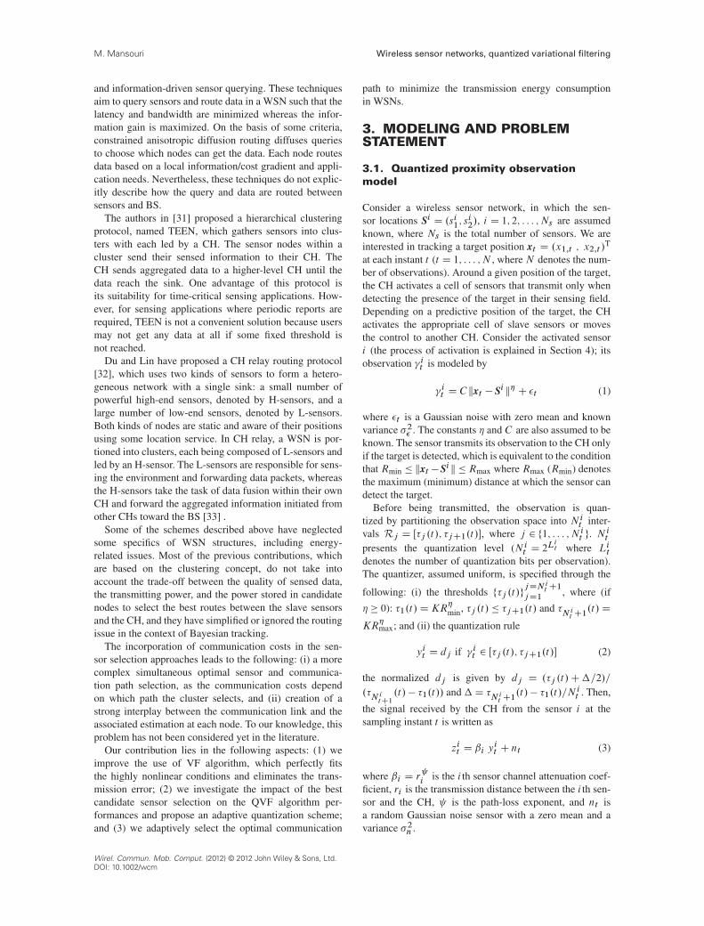
3. MODELING AND PROBLEMSTATEMENT

3.1. Quantized proximity observationmodel

Consider a wireless sensor network, in which the sen-sor locations Si D .si1; s

i2/, i D 1; 2; : : : ; Ns are assumed

known, where Ns is the total number of sensors. We areinterested in tracking a target position xt D .x1;t ; x2;t /T

at each instant t (t D 1; : : : ; N , where N denotes the num-ber of observations). Around a given position of the target,the CH activates a cell of sensors that transmit only whendetecting the presence of the target in their sensing field.Depending on a predictive position of the target, the CHactivates the appropriate cell of slave sensors or movesthe control to another CH. Consider the activated sensori (the process of activation is explained in Section 4); itsobservation � it is modeled by

� it D Ckxt � Sik� C �t (1)

where �t is a Gaussian noise with zero mean and knownvariance �2� . The constants � and C are also assumed to beknown. The sensor transmits its observation to the CH onlyif the target is detected, which is equivalent to the conditionthat Rmin � kxt �Sik �Rmax where Rmax (Rmin) denotesthe maximum (minimum) distance at which the sensor candetect the target.

Before being transmitted, the observation is quan-tized by partitioning the observation space into N it inter-vals Rj D Œ�j .t/; �jC1.t/�, where j 2 f1; : : : ; N it g. N

it

presents the quantization level (N it D 2Lit where Lit

denotes the number of quantization bits per observation).The quantizer, assumed uniform, is specified through the

following: (i) the thresholds f�j .t/gjDN it C1

jD1 , where (if

� � 0): �1.t/DKR�min, �j .t/ � �jC1.t/ and �

N it C1.t/D

KR�max; and (ii) the quantization rule

yit D dj if � it 2 Œ�j .t/; �jC1.t/� (2)

the normalized dj is given by dj D .�j .t/C�=2/=

.�N itC1

.t/� �1.t// and�D �N it C1

.t/� �1.t/=Nit . Then,

the signal received by the CH from the sensor i at thesampling instant t is written as

zit D ˇi yit C nt (3)

where ˇi D r i is the i th sensor channel attenuation coef-

ficient, ri is the transmission distance between the i th sen-sor and the CH, is the path-loss exponent, and nt isa random Gaussian noise sensor with a zero mean and avariance �2n .



3.2. General state evolution model

In this paper, we use a general state evolution modeldescribed in [4,34,35]. The augmented state ˛t D

.xt ;�t ;�t / has a hierarchical model as follows:8<:�t � N .�t j�t�1; N�/�t � W Nn.�t j NS/xt � N .�t ;�t /

(4)

where xt and �t are the target position and its expecta-tion, which are supposed to be Gaussian, and �t is theprecision matrix, which is assumed to have a Wishart distri-bution. These schemes allow the computation of the poste-rior distribution p.˛t jz1Wt /, where z1Wt D fz1; z2; : : : ; zt gdenotes observations gathered until t . The next subsec-tion describes the Bayesian estimation approach via aQVF algorithm.

3.3. Overview of the variational filteringalgorithm

In this section, we assume that the quantization levelis already optimized (Section 4). Hence, the observationmodel is completely defined. The aim of this section is todescribe the target position estimation procedure.

According to model 4, the augmented hidden state isnow ˛t D .xt ;�t ;�t /. We consider the posterior distri-bution p.˛t jz1Wt /, where z1Wt D fz1; z2; : : : ; zt g denotesthe collection of observations gathered until time t . Thevariational approach consists in approximating p.˛t jz1Wt /by a separable distribution q.˛t / D …iq.˛

it / that mini-

mizes the Kullback–Leibler (KL) divergence between thetrue filtering distribution and the approximate distribution,

DKL.qjjp/D

Zq.˛t / log

q.˛t /

p.˛t jz1Wt /d˛t (5)

To minimize the KL divergence subject to constraintRq.˛t /d˛t D …i

Rq.˛it /d˛

it D 1, the Lagrange multi-

plier method is used, yielding the following approximatedistribution [4,34]:

q.˛it / / exp hlogp.zt ;˛t /i…j¤iq.˛jt /(6)

where h:iq.˛

jt /

denotes the expectation operator relative to

the distribution q.˛jt /.With the separable approximate distribution q.˛t�1/ at

time t � 1 taken into account, the filtering distributionp.˛t jz1Wt / is sequentially approximated according to thefollowing scheme:

Op.˛t jz1Wt /Dp.zt j˛t /

Rp.˛t j˛t�1/q.˛t�1/d˛t�1p.zt jz1Wt�1/

/p.zt jxt /p.xt j�t ;�t /p.�t /qp.�t /

with qp.�t /D

Zp.�t j�t�1/q.�t�1/d�t�1

(7)

Therefore, through a simple integral with respect to t�1,the filtering distribution p.˛t jz1Wt / can be sequentiallyupdated. Considering the general state evolution modelproposed above, the evolution of q.t�1/ is Gaussian,namely p.t jt�1/ � N .�t�1;�/. With the definitionof q.t�1/ � N .��t�1;�

�t�1/, qp.t / is also Gaussian,

with the following parameters,

qp.�t /�N .�pt ;�pt /

where �pt D ��t�1 and �pt D .�

�t�1�1C��1/�1

(8)

The temporal dependence is hence reduced to the incor-poration of only one Gaussian component approximationqp.�t�1/. The update and the approximation of the filter-ing distribution p.˛t jz1Wt / are jointly performed, yieldinga natural and adaptive compression [34,36]. According toEquation (6), variational calculus leads to the followingiterative solution:

q.xt / / p.zt jxt /N .xt jh�t i; h�t i/q.�t / / N .�t j��t ;��t /q.�t / / Wn�.�t jS

�t /

q.�t j�t�1/ / N .�pt ;�pt /

(9)

where the parameters are iteratively updated according tothe following scheme:

��t D��1t

�h�t ihxt i C�

pt �

pt

��t Dh�t i C�

pt

n� D NnC 1

S�t D�hxtxT

t i�hxt ih�t iT�h�t ihxt i

TCh�t�Tt iCNS�1��1

�pt D�

�t�1

�pt D

��1t�1 C

N��1��1

(10)

3.4. Predictive distribution calculation

In the Bayesian inference framework, besides updatingthe filtering distribution p.xt jz1Wt /, the activated CH alsoneeds to calculate the predictive distribution p.xt jz1Wt�1/.In fact, the prediction calculation is of great impor-tance for cluster management. The predictive distribu-tion p.xt jz1Wt�1/ can be efficiently updated by variationalinference. Taking into account the separable approximatedistribution q.˛t�1/ / p.˛t�1jz1Wt�1/, we write thepredictive distribution as

p.˛t jz1Wt�1//Zp.˛t j˛t�1/q.˛t�1/d˛t�1

/p.xt ;�t j�t /qp.�t /(11)

The exponential form solution, which minimizes the KLdivergence between the predictive distribution p.˛t jz1Wt�1/and the separable approximate distribution qt jt�1.˛t /,



yields Gaussian distributions for the target state and itsmean and a Wishart distribution for the precision matrix:

qt jt�1.xt / / N .h�t iqtjt�1 ; h�t iqtjt�1/qt jt�1.�t / / N .��

t jt�1;��t jt�1

/

qt jt�1.�t / / Wnx .V�t jt�1

; n�t jt�1

/

(12)

where the hyper-parameters are updated according to thefollowing iterative scheme:

�pt D �

�t�1 (13)

�pt D .�

�t�1�1C N��1/�1

��t jt�1 D ��t jt�1

�1.h�t iqtjt�1hxt iqtjt�1 C�

pt �

pt /

��t jt�1 D h�t iqtjt�1 C�pt

n�t jt�1 D NnC 1

V�t jt�1 D .hxtxTt iqtjt�1 � hxt iqtjt�1h�t i

Tqtjt�1

� h�t iqtjt�1hxt iTqtjt�1

C h�t�Tt iqtjt�1 C

NV�1/�1

(14)

and the predictive expectations of the target state are nowevaluated by the following expressions:

hxt iqtjt�1 D h�t iqtjt�1hxtxT

t iqtjt�1 D h�t i�1qtjt�1

C h�t iqtjt�1h�t iTqtjt�1

(15)Compared with the PF method, the variational approxima-tion dramatically reduces the computational cost and thememory requirements in the prediction phase. In fact, theexpectations involved in the computation of the predictivedistribution have closed forms, avoiding the use of MonteCarlo integration.

3.5. Cluster head determination

The QVF provides, at the sampling instant t , the predictedtarget position xt=t�1 D hxt iqtjt�1 . As shown in Figure 1,on the basis of this predicted information, the CH CHt�1at sampling instant t � 1 selects the next CH CHt . If thepredicted target position hxt iqtjt�1 remains in the vicin-ity of CHt�1, which means that at least four of its slavesensors can detect the target, then CHt D CHt�1. Other-wise, if hxt iqtjt�1 is going beyond the sensing range of thecurrent cluster, then a new CHt is activated, on the basisof the target position prediction hxt iqtjt�1 and its futuretendency.

CHt D arg maxkD1;:::;K

fcos ktdktg (16)

where dkt D khxt iqtjt�1 �LCHktk

and kt D angle.��!hxt�1ihxt iqtjt�1 ;

��!hxt�1iLCHkt

/

Figure 1. Prediction-based CHt activation.

where K is the number of CHs in the neighborhood ofCHt�1 and LCHkt

is the location of the kth neighboring

CHt .As illustrated in Figure 1, the traditional cluster activa-

tion rule [37] activates CH2 to update the filtering distri-bution at time t because it is the closest CH to the targetprediction xt jt�1. But according to the tendency, the targetis very likely to go out of its vicinity in a short time, caus-ing unnecessary hand-off operations. From the decisionrule described by Equation (16), it is CH1 that is acti-vated, as the target is most likely detected by it and wouldstay in its vicinity for a longer period. With the futuretendency of the target taken into consideration, the non-myopic cluster activation rule avoids unnecessary hand-offoperations compared with the traditional one. Therefore,the target tracking accuracy is ensured, and the energyconsumption is minimized as well. Thanks to the varia-tional calculus, communication between CHt�1 and CHtis limited to simply sending the mean and the precision ofq.�t�1/. Therefore, the cluster-based VF algorithm out-performs the classical distributed PF algorithm in resource(energy, bandwidth, and memory) savings, as a large num-ber of particles and corresponding weights are maintainedand propagated in the latter case. With respect to the track-ing accuracy, the VF and PF algorithms approximate thetrue state distribution in different ways. When calculatingthe integral involved in the Bayesian filtering, the PF uses alarge amount of particles whereas the VF introduces hiddenvariables to bypass the difficulty. These random variablesintroduced by the VF act as links that connect the observa-tions to the unknown parameters via Bayes law. The errorpropagation problem is dramatically reduced as approx-imation of the filtering distribution is performed duringobservation incorporation.

To sum up, this CH determination method yields sev-eral advantages. Firstly, the cost of hardware configuration



drops sharply owing to the low cost of slave sensors. Sec-ondly, the required bandwidth and the consumed energyin communication are dramatically reduced. Because thesignal processing task is assigned to only one activatedCH, only the slave sensors belonging to the active CHare required to transmit their observations over short dis-tances. In addition, avoiding CH competition puts anend to unnecessary resource consumption. Only when thehand-off operation occurs does the active CH need tocommunicate the temporal dependence information to thesubsequent CH. However, the occurrence of hand-off oper-ations is reduced by the nonmyopic selective CH activationrule. Furthermore, the temporal dependence information isreduced by the VF algorithm to only the parameters of aGaussian distribution. The limitation of this strategy lies inits vulnerability to external attack. In fact, the activated CHis the only sensor performing tracking algorithm, and noneof its slave sensors would be able to take over this task.

The next section is devoted to the proposed method forselecting the candidate sensors that participate in targettracking.

4. MAXIMUM MUTUALINFORMATION UNDER ENERGYCONSTRAINTS-BASED SENSORSELECTION APPROACH

Because the predicted target position xp.t/ D hxt iqtC1jtat time t is available, it could be used to select the optimalcommunication route. The sensors inside the disk centeredat xp.t/ with radius Rmax are selected, and CH is electedaccording to Equation (16). A sensor node communicateswith CH through the selected route including direct andindirect links. The selected route will be taken accordingto the best communication procedure. The best communi-cation path selection scheme allows CH to get the best copyof the source signal transmitted by the source sensor. TheCH computes for each communication link “sensor–CH” amulti-criteria function (detailed in Section 4.1) and selectsthe optimal communication route, which has the highestMI under energy and node density constraints.

In the next subsection, we detail this criterion and theparameters taken into consideration in order to select thebest communication route between the candidate sensornodes and the CH.

4.1. Maximum mutual information underenergy constraints criterion

The main idea of this criterion for sensor selection is todefine the main parameters that may influence the rele-vance of the sensors cooperation, which are the following:(1) information that can be transferred from candidatesensor i , MI.xt ; zit / (detailed in Section 4.2); (2) itsenergy (E(i)) (detailed in Section 4.3); (3) the transmit-ting energy between one sensor and the CH P.i/ (detailedin Section 4.4); and (4) its density (D(i)) (detailed in

Section 4.5). The problem is how to formulate this criterionfor the CH to select the best sensor that provides satisfieddata of the target and balances the energy level among allsensors and minimum node density in a local cluster. Thecriterion function for node i is given by

arg maxiD1;:::;C

MI.xt ; zit / (17)

s.t P.i/ < P0s.t E.i/ > E0s.t D.i/ < D0

where P0, E0, and D0 (predefined thresholds) are themaximum power, the minimum energy, and the maximumdensity of node constraints, respectively. C represents theset of all pre-selected sensors.

4.2. Computation of the mutualinformation function

The MI function is often used to measure the efficiency of agiven information. The MI function is a quantity measuringthe amount of information that the observable variable ztcarries about the unknown parameter xt . The MI betweenthe observation zit and the source xt is proportional to

MI.xt ; zit / / p.zit jxt / log.p.zit jxt // (18)

The likelihood function .L/ is expressed as

L.si /D p.zit jxt /

D

N it �1XjD0

p��j .t/ < �

it < �jC1.t/

�N�hitdj ; �

2�

�(19)

where

p��j.t/< �

it < �jC1.t/

�D

Z �jC1.t/

�j .t/N�� it.si /; �2n

�d�t

(20)is computed according to the quantization rule defined inEquation (2), in which

�� it.si /DKkxt � sik� (21)

It is worth noting that the expression of the MI givenin Equation (18) depends on the target position xt at thesampling instant t and on the activated sensor i . How-ever, as the target position is unknown, the MI is replacedby its expectation according to the predictive distributionp.xt jzi1Wt�1/ of the target position:

<MI.si / >D Ep.xt jzi1Wt�1/

hMI.si /

i(22)



Computing the above expectation is analyticallyuntractable. However, as the VF algorithm yields aGaussian predictive distribution N .xt I xt=t�1; �t=t�1/,expectation (22) can be efficiency approximated by aMonte Carlo scheme:

<MI.si / >' 1J

PJjD1 MI.Qxjt ; s

i /;

Qxjt �N .xp.t/I xt=t�1;�t=t�1/

where Qxjt is the jth drawn sample at instant t and J is thetotal number of drawn vectors Qxt .

4.3. Computation of the lifetime energy

The energy E is an important parameter in a resource-limited network such as the WSN. It is generally seenas the most important parameter. Indeed, the remainingbattery level appears to be the most important thing in thisparameter, but it is not the only one; it is given by

E.i/D A.i/�APS (23)

where E.i/ is the energy parameter of the sensor i , A isthe available or remaining power in the battery, and APSis the administrator power strategy parameter, which is apercentage defined by the administrator depending on theapplication. As presented in Equation (23), the energy Ecould be just the remaining battery level if no administra-tor power strategy has been defined (APSD 1). In addition,the lower the APS, the longer is the lifetime of the WSN.

4.4. Computation of the sensor nodetransmitting power

The total amount of required transmission power used bythe i th sensor within a cluster [38] is proportional to

P i .t/ / d�i .Nit � 1/

� k si �LCHt k� .N it � 1/

(24)

where di is the transmitting distance (meters) between theCH and the ith sensor, LCHt is the location of the CH atthe sampling instant t , and � is the path-loss exponent.

4.5. Computation of the density of nodes

The network density varies from one deployment toanother and from one node to another within the samedeployment depending on the node distribution. Indeed,the more an agent has neighbors the less is the importanceof its cooperation. For simplicity’s sake, the density D.i/for sensor i is computed by

D.i/DN ith

N ire(25)

whereNth is the theoretical number of nodes and it is givenfrom the ideal distribution of the nodes or the grid distri-bution. Nth corresponds to the number of nodes within theRmax range. Nre is the number of the one-hop neighbors,which means the nodes within the radio range of the nodein question.

The next section is devoted to the developed methodaimed at adaptively selecting the best communication pathbetween the candidate sensor and the CH.

5. BEST COMMUNICATION PATHSELECTION METHOD

In this section, we assume that sensor selection and CHdetermination are already optimized (Sections 2 and 3).The aim of this section is to select the best communica-tion path as well as the highest signal-to-noise ratio (SNR)at the CH by considering the two-hop transmission.

5.1. System model

Figure 2 illustrates the idea of the proposed model. Thecommunication is established between a sensor node andthe CH through the selected relay including direct and indi-rect links. The selected relay is achieved according to theoptimal communication procedure. The CH can get thebest copy of the source signal transmitted by the sourcesensor S, via the optimal communication path selectionscheme. The first one is from the source sensor (directlink), whereas the second one is from the best path asshown in Figure 2. The parameter ˛i shown in Figure 2 isthe channel coefficient between the source sensor S and thei th sensor. ˛i and ˛j and ˇi and ˇj are the flat Rayleighfading coefficients, which are mutually independent andnonidentical for all i and j .

The signal is simply amplified, at the relay sensor i ,

using the gain g D 1=qEs˛

2i CN� , where Es is the trans-

mitted signal energy of the source. It is easy to prove thatthe source to CH SNR of the indirect path, S 7�! i �!

CHS

M

1

2

Target

ii

k

1

2

1

i2

0

k

MM k

Figure 2. Illustration of the diversity network with the optimalcommunication path selection scheme.



CH, can be written as

�S!i!CH D�˛i �ˇi

�˛i C �ˇi C 1(26)

where �˛i D ˛2i .Es=N�/ is the instantaneous SNR of the

source signal at the sensor i , �ˇi D ˇ2i .Ei=E0/ is theinstantaneous SNR of the sensor signal (sensor i ) measuredat the CH, and Ei is the signal-transmitted energy of therelay i .

The optimal communication path will be selected asthe path that achieves the highest source-to-end SNR ofindirect and direct paths. The SNR for the best path isgiven by

�b Dmax.�ˇ0 ; �S!i!CH/iD1:::M (27)

where �ˇ0 D ˇ20.Es=Nn/ is the instantaneous SNRbetween the source and the CH and M is the total numberof links inside the cluster. The upper bound of �S!i!CH isgiven by [39]. Computing the above expression is analyti-cally untractable. However, Equation (27) can be efficiencyapproximated [40] by

�S!i!CH � �i Dmin.�˛i �ˇi / (28)

This approximation simplifies the derivation of the SNRstatistics: cumulative distribution function, probability dis-tribution function (PDF), and moment-generating function(MGF).

The next section is devoted to the developed methodaimed at adaptively selecting the best communication pathbetween the candidate sensor and the CH.

5.2. Error performance analysis

The error probability pe of the best path is given as

pe.�ˇ0 ; �b/D Aerfc�q

B max.�ˇ0 ; �b�

(29)

where erfc.x/ D 2=p R1x exp.�t2/dt and A and B

are dependent on the modulation type. Over the ran-dom variables representing the SNR values of the opti-mal communication path, the average error probability isgiven by

PE D

Z 10

pe.�b/f�bd�b (30)

using the alternative definition of the erfc.x/ function as[41]

erfc.x/D2

Z �2

0exp

�

x2

sin2

!d (31)

and by substituting Equation (31) into Equation (30), weobtain

PE D

Z 10

2

Z �2

0exp

��B�b

sin2

�f�b .�b/d�b

D2

Z �2

0M�b

�B

sin2

�d

(32)

where M�b DR10 f�b .�b/ exp.�s�b/d�b is the MGF of

�b and f�b is the PDF of �b .In order to find thePE, it is necessary to find the PDF and

the MGF of �b . We can write the cumulative distributionfunction of �b as follows:

F�b .�/D P .�b � �/D P .�i � �/P .�ˇ0 � �/iD1:::M

D

24 MYiD1

�1� e��=�i

�35�1� e��=�ˇ0 �(33)

Assuming that �MC1 D �ˇ0 , the PDF can be computedusing the derivative of Equation (33) according to � , sof�b .�/ can be written as

f�b .�/D

MC1XnD1

.�1/.nC1/M�nC2Xk1D1

M�nC3Xk2Dk1C1

: : :

MC1XknDkn�1C1

nYjD1

.e��=�kj /

nXjD1

1

�kj

! (34)

By using the PDF in Equation (34), we can write theMGF as

M�b .s/D

Z 10

e�s�MC1XnD1


M�nC3Xk2Dk1C1

: : :

MC1XknDkn�1C1

nYjD1

.e��=�kj /

nXjD1

1

�kj

!d�

(35)

and the integral can be evaluated in a closed form as

M�b .s/D

MC1XnD1


M�nC3Xk2Dk1C1

MC1XknDkn�1C1

‰n

sC‰n

(36)

where ‰n DPnjD1.1=�kj /.

Substituting Equation (36) in Equation (32) and finaliz-ing the integration using [42], we can write PE in a closed



form as follows:

PE DA

MC1XnD1


M�nC3Xk2Dk1C1

MC1XknDkn�1C1

1�

sB=‰n

1C 1=‰n

!(37)

Outage analysis quantifies the level of performance thatis guaranteed with a certain level of reliability. Proba-bility outage Pout is defined as the probability that thechannel average MI (I ) falls below the required rate R.For the best-path selection diversity networks, Pout can bewritten as

Pout D Pr.I �R/D Pr

�1

2log2.1C �b/�R

�D Pr

��b � 2

2R � 1�DM�b

�22R � 1

�The scheme discussed previously will be referred to asadaptive QVF algorithm; its procedure is summarized inAlgorithm 1.

6. SIMULATION RESULTSANALYSIS

The performance of the proposed algorithms is quantifiedby four criteria:

(1) The tracking accuracy(2) The root mean square errors (RMSE) between the

estimation and the true trajectory of the mobiletarget

Algorithm 1 Pseudo-code of the proposed algorithmInitialization:

(1) Select the candidate sensors that exist within theRmax range.

(2) Select the best communication path betweenthe candidate sensors and the CH according toSection 5.

(3) Quantize sensors’ measurements.(4) Execute the QVF algorithm.

Iterations:

(1) Select sensors that exist within the Rmax range.(2) Compute the predicted target distribution.(3) Compute the MI function based on the predicted

target position using Equation (18).(4) Select the optimal candidate sensors according to

Section 4.(5) Select the best communication path between

the candidate sensors and the CH according toSection 5.

(6) Quantize sensors’ measurements.(7) Execute the QVF algorithm.

(3) The execution time(4) The energy expenditure during the whole tracking

process

The system parameters considered in the following simula-tions are as follows: �D 2 for free space environment, the

−10 0 10 20 30 40 50 60 70 80 90 10020

30

40

50

60

70

80

90

100

110

x1

x2

Sensor Field

True Trajectory

Sensor Nodes

AQVF algorithm

QVF−R algorithm

0 50 100 150 2000

0.5

1

1.5

2

2.5

Time

Err

or e

stim

atio

n

Root Mean Square Error of Target Position Estimation

Error using QVF−R algorithm

RMSE using QVF−R algorithm

Error using AQVF algorithm

RMSE using AQVF algorithm

a) b)

Figure 3. (a) Tracking accuracy between quantized variational filtering (QVF)-R algorithm and the proposed method. (b) Root meansquare error (RMSE) comparison between QVF-R algorithm and the proposed method. AQVF, adaptive QVF.



constant characterizing the sensor range is fixed for sim-plicity to C D 1, the CH noise power is �2n D 10�3, thetotal number of sensors is Ns D 200, the total samplinginstants is N D 200, the sensor noise power is �2� D 10

�4,the maximum sensing range Rmax (the minimum sensingrange Rmin) is fixed to 8:5 m (0 m), and 200 particleswere used in QVF, binary VF (BVF), and quantized PF(QPF) algorithms. All sensors have equal initial batteryenergies of Ei D 1 J. All the simulations shown in thispaper are implemented with MATLAB version 7.1, usinga personal computer with an Intel Pentium 3.4-GHz CPUand 1.0-G RAM.

The approach that uses the QVF algorithm with activat-ing sensors in the circle of radius Rmax for target trackingis referred to as QVF-R.

In the following, we compare the tracking accuracyof the proposed algorithm, with those of the QVF-Ralgorithm, the BVF algorithm [34], and the centralizedQPF algorithm [43]. The quantized proximity observationmodel, formulated in Equation (2), was adopted for theQPF algorithm. One can notice from Figure 3a that, evenwith abrupt changes in the target trajectory, the desiredquality is achieved by the proposed method and outper-forms the QVF-R algorithm. Figure 3b compares their

−10 0 10 20 30 40 50 60 70 80 90 10020

30

40

50

60

70

80

90

100

110

x1

x2

Sensor Field

True Trajectory

Sensor Nodes

AQVF algorithm

BVF algorithm

0 20 40 60 80 100 120 140 160 180 2000

1

2

3

4

5

6

7

Time

Err

or e

stim

atio

n


a) b)

Error using BVF algorithmRMSE using BVF algorithmError using AQVF algorithmRMSE using AQVF algorithm

Figure 4. (a) Tracking accuracy between binary variational filtering (BVF) algorithm and the proposed method. (b) Root mean squareerror (RMSE) comparison between BVF algorithm and the proposed method.

−10 0 10 20 30 40 50 60 70 80 90 10020

30

40

50

60

70

80

90

100

110

x1

x2

Sensor Field

True Trajectory

Sensor Nodes

AQVF algorithm

QPF algorithm

0 50 100 150 2000

1

2

3

4

5

6

7

Time

Err

or e

stim

atio

n


a) b)

Error using QPF algorithmRMSE using QPF algorithmError using AQVF algorithmRMSE using AQVF algorithm

Figure 5. (a) Tracking accuracy between quantized particle filtering (QPF) algorithm and the proposed method. (b) Root mean squareerror (RMSE) comparison between QPF algorithm and the proposed method. AQVF, adaptive quantized variational filtering.



tracking accuracies in terms of RMSE. The performancesof the proposed method demonstrate the effectiveness ofthe sensor selection approach.

RMSEDqE�.x�bx/2� (38)

where x (bx) is the true trajectory (the estimated trajectory).The proposed method and BVF algorithm perfor-

mances are compared in Figure 4. The results confirm theimpact of neglecting the information relevance of sensormeasurements, when we used binary proximity sensors.As can be expected, with the amount of particles increas-ing, the QPF algorithm demonstrates much more accuratetracking at the cost of a higher computation complexity.In particular, the computation time grows proportionallyto the increment of the number of particles. The track-ing accuracy of QPF algorithm is compared with that of

the proposed method in Figure 5. The smaller RMSE ofthe proposed method in comparison with the QPF methodconfirms once again the effectiveness of the proposedmethod in terms of tracking accuracy and the efficiency innon-Gaussian context.

6.1. Root mean square error analysis

The RMSE of the above algorithms may depend on severalfactors such as the transmitting power between the can-didate sensors and the CH, the node density, the sensingrange, the path losses, and the sensor noise variances. Thepurpose of this subsection is to study the impact of thesefactors when comparing the performance of the above-mentioned tracking algorithms. Figure 6a shows the varia-tion of the RMSE with respect to the node density varyingin f50; : : : ; 200g. As can be expected, the RMSE decreases

40 60 80 100 120 140 160 180 2000

2

4

6

8

10

12

14

Density of nodes

RM

SE (

met

er)

RMSE versus Density of nodes

AQVFQVF−RBVFQPF

0 0.05 0.1 0.15 0.2 0.250

1

2

3

4

5

6

7

8

9

10

Nodes noise variances

RM

SE (

met

er)

RMSE versus the Nodes noise variances

AQVFQVF−RBVFQPF

a) b)

Figure 6. (a) Root mean square error (RMSE) versus node density varying in f50; : : : ;200g. (b) RMSE versus node noise variancesvarying in f0; : : : ;0:25g. QVF, quantized variational filtering; BVF, binary variational filtering; QPF, quantized particle filtering.

5 6 7 8 9 10 11 12 130

1

2

3

4

5

6

7

Sensing range (meter)

RM

SE (

met

er)

RMSE versus Sensing range

AQVFQVF−RBVFQPF

50 100 150 2000

2

4

6

8

10

12

Transmitting power (meter)

RM

SE (

met

er)

RMSE versus Transmitting power

AQVFQVF−RBVFQPF

a) b)

Figure 7. (a) Root mean square error (RMSE) versus transmitting power varying in f50; : : : ;200g. (b) RMSE versus sensing rangevarying in f5; : : : ;13g. QVF, quantized variational filtering; BVF, binary variational filtering; QPF, quantized particle filtering.



for all the algorithms when the node density increases. Onecan also note that the proposed adaptive QVF techniqueoutperforms all the other techniques when varying the nodedensity. It is also worth noting that its RMSE decreasesmore sharply than those of the other filtering techniques.Figure 6b plots the RMSE versus the node noise variancesvarying in f0; : : : ; 0:25g, and Figure 7a plots the RMSEwith respect to the nodes transmitting power (varying inf50; : : : ; 200g). From Figure 7b, we can show that whenthe sensing range varies in f5; : : : ; 13g, the error estima-tion decreases. These results confirm that the proposed

method outperforms the classical algorithms when varyingthe simulation conditions.

Figure 8a shows the bit error rate for binary phase shiftkeying with different numbers of paths sensors–CH (M).As can clearly be seen in high-SNR regime, the improve-ment of bit error rate is proportional to the number ofsensors–CH links (M). Figure 8b shows the probabilityoutage (Pout) performance for RD 1 bit/s/Hz.

To evaluate the performances of the proposed method interms of energy consumption, we have used the model pro-posed in [44], in which we assume the following: (i) the

0 5 10 15 20 25 3010−5

10−4

10−3

10−2

10−1

100

SNR (dB)

PE

3 paths4 paths5 paths6 paths

0 5 10 15 20 25 3010−4

10−3

10−2

10−1

100

SNR (dB)

Pou

t

3 paths4 paths5 paths6 paths

a) b)

Figure 8. (a) Error performance for the best-path selection scheme over Rayleigh fading channels. (b) Outage performance for thebest-path selection scheme over Rayleigh fading channels. SNR, signal-to-noise ratio.

0 20 40 60 80 100 120 140 160 180 2000

0.5

1

1.5

2

2.5

3

3.5

4

4.5x 10−5

Time (s)

Ene

rgy

Con

sum

ptio

n

Energy Consumption Comparison

AQVFQVF−R

AQVFQVF−R

0 20 40 60 80 100 120 140 160 180 2000

1

2

3

4

5

6x 10−5

Time (s)

Ene

rgy

Con

sum

ptio

n


a) b)

Figure 9. Energy consumption comparison between adaptive quantized variational filtering (AQVF) and quantized variational filtering(QVF)-U algorithms for (a) LD 3 and (b) LD 4.



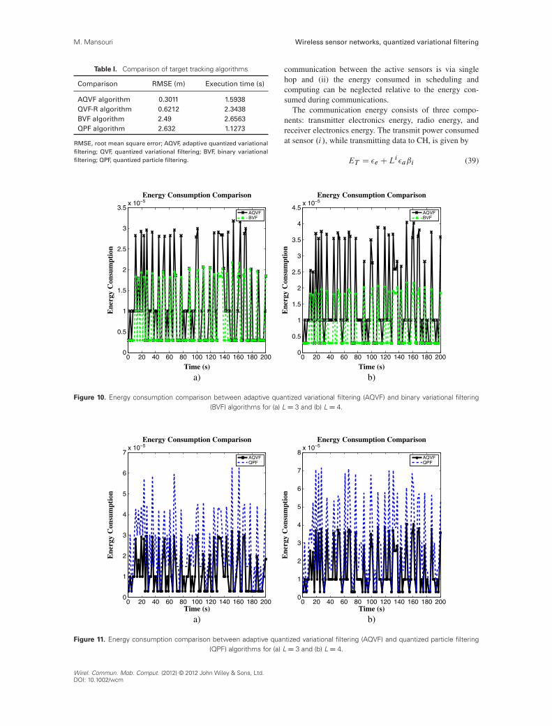
Table I. Comparison of target tracking algorithms

Comparison RMSE (m) Execution time (s)

AQVF algorithm 0.3011 1.5938QVF-R algorithm 0.6212 2.3438BVF algorithm 2.49 2.6563QPF algorithm 2.632 1.1273

RMSE, root mean square error; AQVF, adaptive quantized variationalfiltering; QVF, quantized variational filtering; BVF, binary variationalfiltering; QPF, quantized particle filtering.

communication between the active sensors is via singlehop and (ii) the energy consumed in scheduling andcomputing can be neglected relative to the energy con-sumed during communications.

The communication energy consists of three compo-nents: transmitter electronics energy, radio energy, andreceiver electronics energy. The transmit power consumedat sensor .i/, while transmitting data to CH, is given by

ET D �e CLi �aˇi (39)

0 20 40 60 80 100 120 140 160 180 2000

0.5

1

1.5

2

2.5

3

3.5x 10−5

Time (s)

Ene

rgy

Con

sum

ptio

n


AQVFBVF

0 20 40 60 80 100 120 140 160 180 2000

0.5

1

1.5

2

2.5

3

3.5

4

4.5x 10−5

Time (s)

Ene

rgy

Con

sum

ptio

n


AQVFBVF

a) b)

Figure 10. Energy consumption comparison between adaptive quantized variational filtering (AQVF) and binary variational filtering(BVF) algorithms for (a) LD 3 and (b) LD 4.

0 20 40 60 80 100 120 140 160 180 2000

1

2

3

4

5

6

7x 10−5

Time (s)

Ene

rgy

Con

sum

ptio

n


AQVFQPF

0 20 40 60 80 100 120 140 160 180 2000

1

2

3

4

5

6

7

8x 10−5

Time (s)

Ene

rgy

Con

sum

ptio

n


AQVFQPF

a) b)

Figure 11. Energy consumption comparison between adaptive quantized variational filtering (AQVF) and quantized particle filtering(QPF) algorithms for (a) LD 3 and (b) LD 4.



where �a is the energy dissipated in Joules per bit persquare meter and �e is the energy consumed by the circuitper bit.

The receiving power consumed at i th sensor whenreceiving data from the CH is given by

ER D Li �r (40)

Similarly, the power consumed in sensing is defined by

ES D Li �s (41)

where �s is the energy expending parameter for sensingLi bits of data. Considering the energy model, we choose�a D 100 pJ/bit/m2, �e D 50 nJ/bit, �r D 135 nJ/bit,�s D 50 nJ/bit [34].

From Figures 9–11, we can see that our protocol suc-cessfully balances the trade-off between the energy con-sumption even with several abrupt changes in the trajectorywhere the bit quantization number is L D 3 and L D 4.These results confirm that the proposed method outper-forms the classical algorithms in terms of energy expen-diture during the whole tracking process.

Table I shows the computation complexity, evaluated bythe execution time of the algorithm.

7. CONCLUSIONS

In this paper, we considered an optimal sensor and bestcommunication path selection approach for target track-ing in WSN with quantized measurements. As for eco-nomical reasons, in the hardware layer, the deploymentof quantized sensors greatly saves energy; in the softwarelayer, the proposed algorithm decreases the informationexchanged between sensors. The proposed method pro-vides not only the estimate of the target position usingthe QVF algorithm but also proposes an efficiency can-didate sensor selection method and a best communicationpath selection scheme. The sensor selection approach isbased on MI maximization under energy constraints thatdefine the main parameters that may influence the rele-vance of the sensor cooperation for target tracking, whereasthe best communication path is selected as well as the high-est SNR at the CH. The computation of criteria is based onthe target position predictive distribution provided by theQVF algorithm.

APPENDIX A: VARIATIONALCALCULUS

Assuming that the approximate distribution for themean �t�1 follows a Gaussian model (q.�t�1/ �N .��t�1;�

�t�1/) and taking into account the Gaussian

transition of the mean (p.�t j�t�1/ � N .�t�1; N�/), wegive the predictive distribution of t by

qp.�t / DRp.�t j�t�1/q.�t�1/d�t�1

� N .��t�1; .��t�1�1C N��1/�1/

(A.1)

Let �pt and �pt respectively denote the mean and the pre-cision of the Gaussian distribution qp.�t /: qp.�t / �N .�pt ;�

pt /. According to Equation (6), the approximate

distribution q.�t / is expressed as

q.�t / / exphlogp.z1Wt ;˛t /iq.xt /q.�t / (A.2)

/ exphlogp.˛t jzt /iq.xt /q.�t /

/ exphlogp.zt jxt /C logp.xt j�t ;�t /

C logp.�t /

C log qp.�t /iq.xt /q.�t /

Therefore,

q.�t // qp.�t / exphlogp.xt j�t ;�t /iq.xt /q.�t /

/ qp.�t/ exph�1

2.xt ��t /

T�t .xt ��t /iq.xt /q.�t/

/ qp.�t / exp�1

2

ntrhh�t iq.�t /h.xt ��t /

T

.xt ��t /iq.xt /io

/ exp�1

2

h.�t ��

pt /

T�t .�t ��pt /� 2�

Tt h�t i

�hxt i C�tTh�t i�t

i(A.3)

yielding a Gaussian distribution q.�t /DN .��t ;��t /. Thefirst and second derivatives of the logarithm of q.�t / areexpressed as

@log.q.�t //

@�tD �

1

2

�2�pt .�t ��

pt /� 2h�t ihxt i

C 2h�t i�t

@2log.q.�t //

@�t@�tT D ��

pt � h�t i

The precision ��t and the mean ��t of q.�t / are obtainedas follows:

��t D h�t i C�pt and ��t D �

��1t .h�t ihxt i C�

pt �

pt /

(A.4)

The approximate separable distribution correspondingto �t can be computed following the same reasoning as



above:

q.�t // exphlogp.˛t jzt /iq.xt /q.�t /

/ exphlogp.zt jxt /C logp.xt j�t ;�t /C logp.�t /

C log qp.�t /iq.xt /q.�t /

/ p.�t / exphlogp.xt j�t ;�t /iq.xt /q.�t /

/W2. NV; Nn/j�t j12 exp�

1

2

ntrh�t h.xt ��t /

T

.xt ��t /iq.xt /q.�t /io

/ j�t jNnC1�.2C1/

2

exp�1

2

ntrh�t .hxtxT

t i � hxt ih�t iT

�h�t ihxt iTC h�t�

Tt i C

NV�1/io

(A.5)

which yields a Wishart distribution W2.V�; n�/ for theprecision matrix �t with the following parameters:8̂̂<̂

:̂n� D NnC 1;

V� D .hxtxTt i � hxt ih�t i

T � h�t ihxt iT

C h�t�Tt i C

NV�1/�1

(A.6)

Finally, the approximate distribution q.xt / has the fol-lowing expression:

q.xt / / exphlogp.˛t jzt /iq.�t /q.�t /

/ exphlogp.zt jxt /C logp.xt j�t ;�t /C logp.�t /

C log qp.�t /iq.�t /q.�t /

/ p.zt jxt / exphlogp.xt j�t ;�t /iq.�t /q.�t /

/ p.zt jxt / exp�1

2

ntrhh�t iq.�t /h.xt ��t /

T

.xt ��t /iq.�t /io

/ p.zt jxt /N .h�t i; h�t i/ (A.7)

which does not have a closed form. Therefore, contraryto the cases of the mean �t and the precision �t , inorder to compute the expectations relative to the distri-bution q.xt /, one has to resort to the importance sam-pling method where samples are generated according tothe Gaussian N .h�t i; h�t i/ and then weighted accordingto the likelihood p.zt jxt /.

REFERENCES

1. Chen Y, Zhao Q. On the lifetime of wireless sensornetworks. IEEE Communications Letters 2005; 9(11):976–978.

2. Julier S, Uhlmann J. Unscented filtering and non-linearestimation. In Proceedings of the IEEE, Vol. 92, March2004; 401–422.

3. Djuric P, Kotecha JZJ, Huang Y, Ghirmai T, BugalloM, Miguez J. Particle filtering. IEEE Signal ProcessingMagazine September 2003; 20: 19–38.

4. Snoussi H, Richard C. Ensemble learning onlinefiltering in wireless sensor networks. In IEEE ICCSInternational Conference on Communications Sys-tems, 2006.

5. Teng J, Snoussi H, Richard C. Binary variational fil-tering for target tracking in wireless sensor networks.In IEEE/SP 14th Workshop on Statistical SignalProcessing 2007 (SSP‘07), 2007; 685–689.

6. Patwari N, Ash J, Kyperountas S, Hero III A, MosesR, Correal N. Locating the nodes: cooperative local-ization in wireless sensor networks. IEEE SignalProcessing Magazine 2005; 22(4): 54–69.

7. Patwari N, Hero III A, Perkins M, Correal N, O’deaR. Relative location estimation in wireless sensor net-works. IEEE Transactions on Signal Processing 2003;51(8): 2137–2148.

8. Patwari N, Hero A, Costa J. Learning sensor locationfrom signal strength and connectivity. Secure Localiza-tion and Time Synchronization for Wireless Sensor andAd Hoc Networks 2007: 57–81.

9. Costa J, Patwari N, Hero III A. Distributed weighted-multidimensional scaling for node localization in sen-sor networks. ACM Transactions on Sensor Networks(TOSN) 2006; 2(1): 64.

10. Patwari N. Location estimation in sensor networks,Ph.D. dissertation, Citeseer, 2005.

11. Zhao F, Shin J, Reich J. Information-driven dynamicsensor collaboration for tracking applications.IEEE Signal Processing Magazine 2002; 19(2):61–72.

12. Li J, AlRegib G. Rate-constrained distributed estima-tion in wireless sensor networks. IEEE Transactions onSignal Processing 2007; 55(5 Part 1): 1634–1643.

13. Rubin I, Huang X. Capacity aware optimal activationof sensor nodes under reproduction distortion mea-sures. In Military Communications Conference 2006(MILCOM 2006), 2006; 1–8.

14. Quan Z, Sayed A. Innovations-based sampling overspatially-correlated sensors. In IEEE InternationalConference on Acoustics, Speech and Signal Process-ing 2007 (ICASSP 2007), Vol. 3, 2007.

15. Bian F, Kempe D, Govindan R. Utility-based sen-sor selection. In The Fifth International Conferenceon Information Processing in Sensor Networks 2006(IPSN 2006), 2006; 11–18.

16. Hintz K. A measure of the information gainattributable to cueing. IEEE Transactions on Systems,Man and Cybernetics 1991; 21(2): 434–442.

17. Manyika J, Durrant-Whyte H. Data Fusion and SensorManagement: A Decentralized Information-Theoretic



Approach. Prentice Hall PTR: Upper Saddle River, NJ,1995.

18. Liu J, Reich J, Zhao F. Collaborative in-networkprocessing for target tracking. EURASIP Journal onApplied Signal Processing 2003; 2003: 378–391.

19. Ertin E, Fisher J, Potter L. Maximum mutual informa-tion principle for dynamic sensor query problems. InInformation Processing in Sensor Networks. Springer:Heidelberg, 2003; 558–558.

20. Yao K, Hudson R, Reed C, Chen D, Lorenzelli F.Blind beamforming on a randomly distributed sen-sor array system. IEEE Journal on Selected Areas inCommunications 1998; 16(8): 1555–1567.

21. Chu M, Haussecker H, Zhao F. Scalable information-driven sensor querying and routing for ad hoc het-erogeneous sensor networks. International Journalof High Performance Computing Applications 2002;16(3): 293–313.

22. Wang H, Yao K, Pottie G, Estrin D. Entropy-basedsensor selection heuristic for target localization. InProceedings of the 3rd International Symposium onInformation Processing in Sensor Networks ACM,2004; 45.

23. Dong Q. Maximizing system lifetime in wirelesssensor networks. In Fourth International Symposiumon Information Processing in Sensor Networks 2005(IPSN 2005), 2005; 13–19.

24. Shah R, Rabaey J. Energy aware routing for low energyad hoc sensor networks. In IEEE Wireless Communi-cations and Networking Conference (WCNC), Vol. 1.IEEE: Piscataway, NJ, USA, 2002; 350–355.

25. Li Q, Aslam J, Rus D. Online power-aware rout-ing in wireless ad-hoc networks. In Proceedings ofthe 7th Annual International Conference on MobileComputing and Networking, ACM, 2001; 107.

26. Chang J, Tassiulas L. Maximum lifetime routing inwireless sensor networks. IEEE/ACM Transactions onNetworking (TON) 2004; 12(4): 609–619.

27. Liu J, Zhao F, Petrovic D. Information-directed rout-ing in ad hoc sensor networks. In Proceedings of the2nd ACM International Conference on Wireless SensorNetworks and Applications, ACM, 2003; 88–97.

28. Sung Y, Misra S, Tong L, Ephremides A. Coopera-tive routing for distributed detection in large sensornetworks. IEEE Journal on Selected Areas in Commu-nications 2007; 25(2): 471–483.

29. Intanagonwiwat C, Govindan R, Estrin D. Directeddiffusion: a scalable and robust communicationparadigm for sensor networks. In Proceedings ofthe 6th Annual International Conference on MobileComputing and Networking, ACM, 2000; 56–67.

30. Braginsky D, Estrin D. Rumor routing algorithm forsensor networks. In Proceedings of the 1st ACM

International Workshop on Wireless Sensor Networksand Applications, ACM, 2002; 22–31.

31. Lou W. An efficient N -to-1 multipath routing proto-col in wireless sensor networks. In IEEE InternationalConference on Mobile Ad Hoc and Sensor SystemsConference 2005, IEEE, 2005; 8–672.

32. Du X, Lin F. Improving routing in sensor networkswith heterogeneous sensor nodes. In Vehicular Tech-nology Conference 2005 (VTC 2005)—Spring 2005IEEE 61st, Vol. 4. IEEE, 2005; 2528–2532.

33. Akkaya K, Younis M. A survey on routing protocolsfor wireless sensor networks. Ad Hoc Networks 2005;3(3): 325–349.

34. Teng J, Snoussi H, Richard C. Binary variationalfiltering for target tracking in sensor networks. IEEEWorkshop on Statistical Signal Processing Aug. 2007:685–689.

35. Vermaak J, Lawrence N, Perez P. Variational infer-ence for visual tracking. In 2003 IEEE ComputerSociety Conference on Computer Vision and PatternRecognition, 2003. Proceedings, Vol. 1, 2003.

36. Snoussi H, Richard C. Ensemble learning online fil-tering in wireless sensor networks. In 10th IEEESingapore International Conference on Communica-tion systems 2006 (ICCS 2006), 2006; 1–5.

37. Yang H, Sikdar B. A protocol for tracking mobiletargets using sensor networks. In Proceedings of theFirst IEEE International Workshop on Sensor NetworkProtocols and Applications 2003, 2003; 71–81.

38. Cui S, Goldsmith A, Bahai A. Energy-constrainedmodulation optimization. IEEE Transactions on Wire-less Communications 2005; 4(5): 2349–2360.

39. Ikki S, Ahmed M. Performance analysis of cooperativediversity wireless networks over Nakagami-m fadingchannel. IEEE Communications Letters 2007; 11(4):334.

40. Valenzuela R. A statistical model for indoor multi-path propagation. IEEE Journal on Selected Areas inCommunications 1987; 5(2): 128–137.

41. Simon M, Alouini M. Digital Communication OverFading Channels. Wiley-IEEE Press: New York, 2005.

42. Papoulis A, Pillai S. Probability, Random Variablesand Stochastic Processes. McGraw-Hill Education(India) Pvt Ltd, 2002.

43. Zuo L, Niu R, Varshney P. A sensor selection approachfor target tracking in sensor networks with quantizedmeasurements. In Proceedings of the 2007 IEEE Inter-national Conference on Acoustics, Speech, and SignalProcessing, II; 2521 –2524.

44. Heinzelman W, Chandrakasan A, Balakrishnan H.Energy-efficient communication protocol for wirelessmicrosensor networks. In Proceedings of the 33rdHawaii International Conference on System Sciences,



Vol. 8. IEEE Computer Society: Washington, DC,USA, 2000; 8020.

AUTHOR’S BIOGRAPHY

Majdi Mansouri was born 11November 1982 in Kasserine, Tunisia.He received the Diplom-Ingenieurdegree in 2006 from High Schoolof Communications of Tunis(SUP’COM) and the MS degree in2008 from High school of Elec-tronic, Informatique and Radiocom-

munications in Bordeauxx (ENSEIRB). He received

the PhD degrees in 2011 from Troyes University of Tech-nology, France. He is currently a postdoctoral researchassociate at Texas A&M University at Qatar. His currentresearch interests include statistical signal processing andwireless sensors networks. Mansouri is the author of over25 papers.


optimal sensor and path selection for target tracking in ... ltering by jointly selecting the...

Documents