generating optimal scheduling for wireless sensor...
TRANSCRIPT

Generating Optimal Scheduling for Wireless Sensor Networksby Using Optimization Modulo Theories Solvers
Gergely Kovasznai, Csaba Biro and Balazs Erdelyi
IoT Research InstituteEszterhazy Karoly University
Eger, Hungaryiot.uni-eszterhazy.hu/en
SMT 2017July 22, 2017
Heidelberg, Germany
Gergely Kovasznai, Csaba Biro and Balazs Erdelyi WSN Optimization by OMT Solvers

IoT applications, WSNs
Internet of Things (IoT) includes the use of small, inexpensive,self-powered devices that can sense their environment. Typically in
agriculture,
industry,
security,
environmental and habitat monitoring,
traffic monitoring,
military,
etc.
Typically, they communicate wirelessly.
Gergely Kovasznai, Csaba Biro and Balazs Erdelyi WSN Optimization by OMT Solvers

Outline
Security and dependability constraints: coverage, evasive andmoving target
Lifetime maximization
SMT-based approaches
OMT problem formalization
WSN simulation
Benchmarks
Experiments
Conclusions and future work
Gergely Kovasznai, Csaba Biro and Balazs Erdelyi WSN Optimization by OMT Solvers

Security and dependability constraints: coverage
How well the sensors observe the physical environment? Two main types:
Area coverage to cover a given area of interest;
Point coverage to cover a set of target points.
[M. Cardei. Coverage problems in sensor networks. Handbook of Combinatorial Optimization, 2013.]
Point coverage can be used to simulate area coverage by using pointsthat approximate an area.
Gergely Kovasznai, Csaba Biro and Balazs Erdelyi WSN Optimization by OMT Solvers

Security and dependability constraints: evasive and movingtarget constraints
Additional security requirements in critical systems and in militaryapplications, in order to protect sensor nodes to be damaged, detected orattacked.
Evasive constraint. To prohibit the sensor nodes to be active for too long.
Moving target constraint. Not to cover critical target points by the samesensor node for too long.
Gergely Kovasznai, Csaba Biro and Balazs Erdelyi WSN Optimization by OMT Solvers

Lifetime maximization
The aim is to maximize the WSN’s lifetime.
Why?
Sensor nodes are self-powered and have limited power supply.
How?
By sending certain sensor nodes into sleep mode and waking themup later on, in a synchronized way.
Let’s generate a sleep/wake-up scheduling which does not violate theconstraints at any time and provides a maximal lifetime for the WSN!
Gergely Kovasznai, Csaba Biro and Balazs Erdelyi WSN Optimization by OMT Solvers

Heuristic optimization approaches for coverage solving
Most of previous works deal WSN lifetime maximization as anoptimization problem by applying heuristics.[M. Cardei, D. Ding-Zhu. Improving wireless sensor network lifetime through
power aware organization. Wireless Networks, 2005.]
[D. Tian, N. D. Georganas. A coverage-preserving node scheduling scheme for
large wireless sensor networks. WSNA, 2002.]
They scale up to a few hundred sensor nodes and tens of targetpoints.
They sometimes sacrifice 100% precise coverage.
They focus on the coverage problem, without giving attention toother security/dependability constraints (e.g. evasive, movingtarget).
Gergely Kovasznai, Csaba Biro and Balazs Erdelyi WSN Optimization by OMT Solvers

SMT-based approaches
A few previous works apply SMT solving to generate a sleep/wake-upscheduling that respects WSN constraints.
[K. Weiqiang et al. An SMT-based accurate algorithm for the K-coverage
problem in sensor network. UBICOMM, 2014.]
Focuses only on coverage. Deals only with homogeneous nodes. Reportsexperiments with Z3.
[Q. Duan et al. Provable configuration planning for wireless sensor networks.
CNSM, 2012.]
Addresses several constraints. Deals only with homogeneous nodes.Reports experiments with Yices. Scales up to hundreds of nodes.
None of them addresses lifetime maximization.Shall we try to apply OMT solvers?
Gergely Kovasznai, Csaba Biro and Balazs Erdelyi WSN Optimization by OMT Solvers

What is the plan?
1 Let us introduce an OMT formalization of the lifetime maximizationproblem for WSNs where
all of the coverage, evasive and moving target constraints areaddressed,sensor nodes are heterogeneous (i.e., they have different sensingranges).
2 Let us perform experiments with existing OMT solvers:OptiMathSAT, Z3, Symba.[R. Sebastiani, P. Trentin. OptiMathSAT: A tool for optimization modulo
theories. CAV, 2015.]
[N. Bjørner et al. µZ - An optimizing SMT solver. TACAS, 2015.]
[Y. Li et al. Symbolic optimization with SMT solvers. POPL, 2014.]
3 Let us provide new and practical OMT benchmarks for the SMTcommunity.
Gergely Kovasznai, Csaba Biro and Balazs Erdelyi WSN Optimization by OMT Solvers

OMT formalization
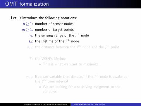
Let us introduce the following notations:
n ≥ 1: number of sensor nodes
m ≥ 1: number of target points
ri : the sensing range of the i th node
Li : the lifetime of the i th node
di,j : the distance between the i th node and the jth point
T : the WSN’s lifetime
This is what we want to maximize.
wi,t : Boolean variable that denotes if the i th node is awake atthe tth time interval
We are looking for a satisfying assigment to thevariables.
Gergely Kovasznai, Csaba Biro and Balazs Erdelyi WSN Optimization by OMT Solvers
OMT formalization
Let us introduce the following notations:
n ≥ 1: number of sensor nodes
m ≥ 1: number of target points
ri : the sensing range of the i th node
Li : the lifetime of the i th node
di,j : the distance between the i th node and the jth point
T : the WSN’s lifetime
This is what we want to maximize.
wi,t : Boolean variable that denotes if the i th node is awake atthe tth time interval
We are looking for a satisfying assigment to thevariables.
Gergely Kovasznai, Csaba Biro and Balazs Erdelyi WSN Optimization by OMT Solvers

OMT formalization – Lifetime constraint
For each node, the number of time intervals at which the node is awakemust not exceed the node’s lifetime.
∀i (1 ≤ i ≤ n).T∑t=1
wi,t ≤ Li
SMT-LIB formalization:
(<=
(+ (boolToInt (w i 0))(boolToInt (w i 1)). . . (boolToInt (w i T )) )
(L i) )
Gergely Kovasznai, Csaba Biro and Balazs Erdelyi WSN Optimization by OMT Solvers

OMT formalization – K -coverage constraint
Each point is covered by at least K ≥ 1 sensor nodes.
∀j , t (1 ≤ j ≤ m, 1 ≤ t ≤ T ).∑i∈Sj
wi,t ≥ K
where Sj = {i | di,j ≤ ri} is the set of nodes which are able to cover thejth point.
SMT-LIB formalization:
(>=
(+ (boolToInt (covers0 j At t))(boolToInt (covers1 j At t)). . . (boolToInt (coversnj At t)) )
K )
Gergely Kovasznai, Csaba Biro and Balazs Erdelyi WSN Optimization by OMT Solvers

Illustration – K -coverage constraint
(a) t = 0 (b) t = 1 (c) t = 2
Figure: Sleep/wake-up scheduling of sensor nodes for 2-coverage and evasiveconstraint with E = 2. The active nodes (blue dots) are monitoring the targetpoints (green dots).
Gergely Kovasznai, Csaba Biro and Balazs Erdelyi WSN Optimization by OMT Solvers

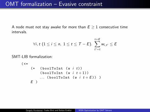
OMT formalization – Evasive constraint
A node must not stay awake for more than E ≥ 1 consecutive timeintervals.
∀i , t (1 ≤ i ≤ n, 1 ≤ t ≤ T − E ).t+E∑t′=t
wi,t′ ≤ E
SMT-LIB formalization:
(<=
(+ (boolToInt (w i t))(boolToInt (w i t + 1)). . . (boolToInt (w i t + E )) )
E )
Gergely Kovasznai, Csaba Biro and Balazs Erdelyi WSN Optimization by OMT Solvers

OMT formalization – Moving target constraint
Some critical points may require not to be covered by the same sensornode for more than M ≥ 1 consecutive time intervals.
∀j ∈ CR, ∀i ∈ Sj , ∀t (1 ≤ t ≤ T −M).t+M∑t′=t
wi,t′ ≤ M
where CR ⊆ {j | 1 ≤ j ≤ m} is the set of critical points.
SMT-LIB formalization: Similar to the one for the evasive constraint.
Gergely Kovasznai, Csaba Biro and Balazs Erdelyi WSN Optimization by OMT Solvers

OMT formalization – Objective function
The aim is to maximize the WNS’s lifetime.
max : T
SMT-LIB formalization:
For Z3:
(maximize T)
For OptiMathSAT:
(maximize T :local -lb 0 :local -ub T )
where T =∑n
i=1 Li works as a time horizon for the WSN.
For Symba:
(=> $constraints (<= T TOpt) )
Gergely Kovasznai, Csaba Biro and Balazs Erdelyi WSN Optimization by OMT Solvers

OMT benchmarks – WSN simulation
For simulating WSNs, we chose an IEEE 802.15.4 compatible sensornode that is able to communicate wirelessly and has common parameterssuch as a 3V power supply.A good example is the commonly used sensor node MICAz.
Such sensor nodes are provided with an RF transceiver with an estimatedrange of 100m, such as the commonly used CC2420.
Gergely Kovasznai, Csaba Biro and Balazs Erdelyi WSN Optimization by OMT Solvers

OMT benchmarks – WSN simulation
The manufacturer of CC2420 publish data about 8 performance levels.We need to calculate the sensing range for each performance level.
PA LEVEL Output Power P Power Consumption I Estimated Range r(mW ) (mA) (m)
31 1.000 17.4 12027 0.794 16.5 ?23 0.501 15.2 ?19 0.316 13.9 ?15 0.200 12.5 ?11 0.100 11.2 ?7 0.032 9.9 ?3 0.003 8.5 ?
We can calculate the minimum range from the minimum output power:
rmin =√Pminr2
max
The estimated range r for the power consumption I can be calculated asfollows:
r =rmax − rmin
Pmax − Pmin(I − Imin) + rmin
Gergely Kovasznai, Csaba Biro and Balazs Erdelyi WSN Optimization by OMT Solvers

OMT benchmarks – WSN simulation
The manufacturer of CC2420 publish data about 8 performance levels.We need to calculate the sensing range for each performance level.
PA LEVEL Output Power P Power Consumption I Estimated Range r(mW ) (mA) (m)
31 1.000 17.4 12027 0.794 16.5 10923 0.501 15.2 9219 0.316 13.9 7515 0.200 12.5 5811 0.100 11.2 417 0.032 9.9 253 0.003 8.5 6.75
We can calculate the minimum range from the minimum output power:
rmin =√Pminr2
max
The estimated range r for the power consumption I can be calculated asfollows:
r =rmax − rmin
Pmax − Pmin(I − Imin) + rmin
Gergely Kovasznai, Csaba Biro and Balazs Erdelyi WSN Optimization by OMT Solvers

OMT benchmarks
A network grid of 600 meters by 600 meters. Random locations forsensor nodes and target points. Random performance levels.
We generated two benchmark sets:
Harder benchmarks: 10 sensor nodes, 4 target points, 2-coverageconstraint, evasive constraint with E = 3, and movingtarget constraint with M = 2.
Easier benchmarks: 10 sensor nodes, 2 target points, 1-coverageconstraint, evasive constraint with E = 2, and movingtarget constraint with M = 1.
Within each benchmark set, we generated1 20 benchmarks with all the constraints enabled,2 20 benchmarks with only the moving target constraint disabled, and3 20 benchmarks with only the evasive constraint disabled.
3 variants of each benchmark instance: for OptiMathSAT, Z3, andSymba, respectively.
Gergely Kovasznai, Csaba Biro and Balazs Erdelyi WSN Optimization by OMT Solvers

Experiments
Experiments were run on 3.60 GHz 8-core CPU with 8 GB memory. Timelimit: 600 seconds. Memory limit: 3 GB.
Results for the harder benchmarks over QF UFLIA:
Solver #SAT/UNS #TO Opt Time Space #Crash
All OptiMathSAT 11/5 4 73 245.5 440.3constraint Z3 2/5 13 72 393.6 449.8on Symba 1/5 14 2 423.1 461.9
Moving OptiMathSAT 10/5 5 74 215.8 314.8target Z3 7/5 8 73 258.2 408.3off Symba 4/5 11 60 393.5 439.1
Evasive OptiMathSAT 12/4 3 74 149.0 286.5 1off Z3 7/5 8 72 265.2 468.5
Symba 5/5 10 60 355.6 475.0
Gergely Kovasznai, Csaba Biro and Balazs Erdelyi WSN Optimization by OMT Solvers

Experiments
Results for the easier benchmarks over QF UFLIA:
Solver #SAT/UNSAT #TO Opt Time Space
All Z3 20/0 0 226 63.1 493.1constraints OptiMathSAT 12/0 8 159 277.8 520.7on Symba 9/0 11 159 484.9 436.2
Moving Z3 20/0 0 226 49.2 333.7target OptiMathSAT 11/0 9 130 311.3 476.1off Symba 9/0 11 159 488.8 340.0
Evasive Z3 20/0 0 226 50.8 300.0off Symba 19/0 1 226 324.8 334.1
OptiMathSAT 12/0 8 159 344.1 488.2
Gergely Kovasznai, Csaba Biro and Balazs Erdelyi WSN Optimization by OMT Solvers

Experiments
Results for the easier benchmarks over QF UFLRA:
Solver #SAT/UNSAT #TO Opt Time Space
All Z3 19/0 1 226 87.7 497.1constraints Symba 18/0 2 226 223.4 578.5on OptiMathSAT 12/0 8 159 277.0 507.4
Moving Z3 20/0 0 226 41.4 318.9target Symba 20/0 0 226 172.5 393.0off OptiMathSAT 11/0 9 130 310.6 469.9
Evasive Z3 20/0 0 226 36.2 284.4off Symba 20/0 0 226 128.9 340.5
OptiMathSAT 11/0 9 159 345.2 467.5
Gergely Kovasznai, Csaba Biro and Balazs Erdelyi WSN Optimization by OMT Solvers

Conclusion and future work
Conclusions:
OptiMathSAT provides the most stable performance and scalesthe best
Z3 is efficient on fewer target points and lower parameter values
Symba provides convincing performance over real numbers
Future work:
To do experiments with different parameter settings for the OMTsolvers
To provide benchmarks with larger network grid and higher numberof nodes/points
To come up with an specialized OMT approach for WSN-likeoptimization problems
Based on the energy-consumption values, we could predict when theWSN runs out of energyPreliminary, convincing results for 40-50 nodes
Gergely Kovasznai, Csaba Biro and Balazs Erdelyi WSN Optimization by OMT Solvers