cellular automata urban growth simulation and …jshan/publications/2005/geocompute...ground truth...

1

Cellular Automata Urban Growth Simulation and Evaluation - A Case Study of Indianapolis

Sharaf Alkheder and Jie Shan

Geomatics Engineering, School of Civil Engineering, Purdue University

550 Stadium Mall Drive, West Lafayette, IN 47907, USA Phone: (765) 494-2168; Fax: (765) 496-1105

Email: {salkhede, jshan}@purdue.edu

Abstract The objective of this paper is to develop and implement a Cellular Automata (CA) algorithm to simulate urban growth process. Indianapolis city, Indiana is selected as a case study to simulate its urban growth over the last three decades. Urban growth simulation for an artificial city is carried out first. It evaluates a number of urban sprawl parameters including the size and shape of neighborhood besides testing different types of constraints on urban growth simulation. The results indicate that circular-type neighborhood shows smoother but faster urban growth as compared to nine-cell Moore neighborhood. Also, CA rules definition is critical stage in simulating the urban growth pattern in a close manner to reality. Next step includes running the developed CA simulation over classified remotely sensed historical imagery in a developed ArcGIS toolkit. A set of crisp rules are defined and calibrated based on real urban growth pattern. Uncertainty analysis is performed to evaluate the accuracy of the simulated results as compared to the historical ground truth images. Evaluation shows promising results represented by the high average accuracies achieved. The average accuracy for the predicted growth images 1987 (for a period of 5 years) and 2003 (for a period of 10 years) is over 80 %. Modifying CA growth rules over time to match the growth pattern changes is important to obtain accurate simulation. This modification is based on the urban growth relationship for Indianapolis over time as can be seen in the historical images. The feedback obtained from comparing the simulated and ground truth images is crucial in identifying the optimal set of CA rules for reliable simulation and calibrating growth steps.

1. Introduction Extensive research efforts are behind the development of dynamic modelling domain for a better understanding of the spatial effect of urban growth process and its applications (Meaille and Wald, 1990; Batty and Xie, 1994a and 1994b). Most of the developed models are cell-based that can be categorized as models that uses cellular automata (White and Engelen, 1997; Batty et al., 1999), models that uses transition probabilities in a class transition matrix (Turner, 1987; Veldkamp and Fresco, 1996) and GIS weighted overlay models (Pijanowski et al., 1997). Models based on cellular automata are the most

2

impressive in term of their technological evolution in connection to urban applications (Yang and Lo, 2003). Cellular Automata (CA) can be referred to as one of the Artificial Intelligence (AI) tools (Tsoukalas and Uhrig, 1997). The definition of CA rules is still a research issue, despite the emergence of CA as a powerful visualization tool in urban growth simulation (Batty, 1998). Urban CA is developed largely through trial and error which makes the CA models essentially heuristic (Wu, 2002). Calibration and validation of CA models had been neglected issues till recent research efforts start focusing on this topic. For example Multicriteria evaluation (MCE) was used by Wu and Webster (1998) to evaluate the CA model parameters. Clark et al. (1997) used visual tests to evaluate the CA simulation results. Calibration and validation are two critical issues to be fully researched to develop CA as reliable procedure for urban simulation (Wu, 2002). Geographic Information Science (GIS) as a rich environment of spatial supported tools is suitable to implement the developed CA rules in a dynamic simulation process to produce visual presentation of the simulation results. Coupling GIS programming capabilities with CA will provide a flexible framework for programming and running the dynamic spatial model (Li and Yeh, 2000). Our work focuses on designing and calibrating CA algorithm to simulate urban growth in Indianapolis in GIS environment over time period of thirty years. Many growth parameters related to neighborhood and new growth constraints are tested to identify their effect on the growth process in artificial city environment. We concentrate on CA rules definition and refining through error backpropagation principle. Simulation results of growth pattern are evaluated through designing a special evaluation tool that takes spatial distribution of urban structure into consideration. Growth pattern over the city derived from the real growth data is used as a basis of CA rules update to match any growth jump over time. 2. Principle of Cellular Automata The most common definition is presenting CA as a dynamical discrete system in space and time that operates on a uniform grid-based space through implementing local rules. CA is an iterative computational process. The future cell state is determined based on a neighborhood function giving that the established transition rules and defined constraints are achieved. Any CA system is composed of four components – cells (pixels in the GIS discrete grid artificial world), states (land use classes in classified images), neighborhood (Moore, circle ...etc) and transition rules. CA was originally introduced by Ulam and von Neumann in 1940’s as a framework to study the behaviour of complex systems (von Neumann, 1966). Sipper (1997) refers to the grid cellular array as n-dimensional where n = 1, 2, 3 are used in practice. One- and two-dimensional grids are the most common. Sipper mentioned that the identical rule contains in each cell is essentially a finite state machine. It usually specified in the form of a rule table or transition function with an entry for every possible neighborhood configuration of states. According to Codd (1968), Sipper (1997) provides a formal definition of 2-D cellular automata. Let I represent the integers set. To obtain a cellular space associated with the set IxI; the neighborhood function for cell α over the set IxI can be defined as in Equation 1.

3

{ }1 2( ) , ,.............., ng α α δ α δ α δ= + + + (1)

where; ( , ) x i I Iα δ ∈ and iδ (i=1…n) represents index of the neighborhood cells. For example, if we have 3x3 Moore neighborhood then α represents the center pixel and

iα δ+ (i=1 to 8) represents the 8 neighboring cells surroundingα . The finite automaton is defined as 0( , , )V v f , given that 0v represents distinguished element of cellular states V . The symbol f stands for the local transition function that is subject to the restriction in Equation 2. In the case of 2-state cellular space (urban vs. non-urban), V is 2 representing the total number of states we have while 0v represents either urban or non-urban state. Local transition function f evaluates the effect that the neighborhood has on identifying the future state ofα .

0 0 0( ,.........., )f v v v= (2)

Equation 2 indicates that f is a transition function from n-tuples of elements of V into V .

The neighborhood state function :t nh IxI V→ is defined as in Equation 3.

1( ) ( ( ), ( ),........, ( ))t t t tnh v v vα α α δ α δ= + + (3)

Given that 1( ( ), ( ),........, ( ))t t t

nv v vα α δ α δ+ + are the current states (time = 0) of the pixel under consideration and its neighborhood pixels. The relation between cell α sate at time (t+1) and its neighborhood states at time t can be expressed as shown in Equation 4.

1( ( )) ( )t tf h vα α+= (4)

( ( ))tf h α represents the transition rules defined on the neighborhood in CA simulation

system represented by the IF…THEN rules presented to drive the simulation process. In the same example of 2-state cellular space and the 3x3 Moore neighborhood,

( )th α represents the states inside the Moore kernel at starting time t. The function ( ( ))tf h α implements the crisp IF...THEN rules over ( )th α to identify the future α state at

time t+1. The global transition function F over C - represents all the configurations or allowable states at time t ( 2 in the above example) for a given cellular space - for all x I Iα ∈ can be defined as in Equation 5.

( )( ) ( ( ))F c f hα α= (5)

4

For eachα , ( 0, 1,....)c c represents the states’ configurations in the neighborhood ofα at

time t. The updated c at time (t+1) - 1tc + - will be evaluated as 1 ( )t tc F c+ = . The definition of the neighborhood region over the x I I cellular space as a connected set of pixels around α can be presented as a city-block metricτ defined by Equation 6:

( , ) +x x y yα β α βτ α β = − − (6)

Given that ( , )x yα αα = and ( , )x yβ ββ = . The function ( , )τ α β defined the neighborhood

connected set of pixels around pixel α such that{ }0x c( )I I vα α∈ ≠ . In the above example of 3x3 Moore neighborhood, τ represents the dimension of the square neighborhood region by 3 in the x-direction and 3 in the y-direction of total 9 cells. In the case of circular-like neighborhood, τ will represent the dimension of the circular neighborhood region represented by the enclosed number of pixels within the circular area. 3. Artificial City Simulation In this section we will implement the CA concept to simulate the urban growth for an artificial city in order to test number of modelling parameters that affect the urban growth simulation. These parameters include the size and shape of neighborhood and the effect of different constraints on the simulation process. 3.1 Size and Shape of Neighborhood The size and shape of neighborhood has an effect on the urban growth rate and results. In order to test the effect of size and shape of neighborhood kernel on the simulated growth results, an example of 2-state land use binary image (urban vs. non urban) is used as shown in Figure 1. The total size of the image is 200x200 pixels of which 60x60 pixels is defined as an urban area. CA simulation is implemented on the input image using two different neighborhood configurations (a. Moore (3x3) and b. Circular- like) as explained in Figure 2. Simple crisp IF…THEN rules are used to drive the simulation using the two different neighborhood kernels:

• IF the tested pixel is non-urban surrounded by 3 or more urban pixels, THEN change it to urban.

• IF the tested pixel is urban, THEN keep it urban. Figure 3 summarizes the simulated urban growth results for Moore and Circular- like neighborhoods after specific number of growth steps. The results indicate two important remarks. First, the growth rate is higher for Circular- like neighborhood as compared to Moore neighborhood. This is obvious in the figure where it takes only 34 steps for circular kernel to reach the same growth achieved by Moore kernel after 70 steps. Growth equality between the two neighborhoods’ output images means equal urban area represented in same number of red pixels for both images. Each growth step represents scanning the whole image once and updating all image pixels based on CA rules.

5

Figure 1. Two-state land use binary image as input for CA simulation

Figure 2. Two-neighborhood configurations used for CA simulation This result indicates the effect of the selected size of neighborhood on the urban growth simulation results. The second note is considering the effect of the shape of neighborhood on the simulation results. As can be seen clearly that using Circular- like neighborhood produces smoother growth pattern - obviously seen at the edges of urban/non-urban regions - as compared to Moore neighborhood. Such smoothness can be referred to the less growth irregularities produced in the case of circular kernel where the growth trend start by filling the gaps between developed pixels to reach the stability level. The results of this binary artificial urban growth simulation suggest that neighborhood has effect on the simulation results if not selected in a proper way. 3.2 Artificial City Urban Growth Simulation This section will mimic the reality using artificial urban growth simulation through introducing more complex structure of urban system. A complete working example is provided using predefined neighborhood configuration and a set of CA crisp growth rules. Figure 4 presents the image of size 200x200 pixels that used as an input to the CA simulation algorithm. Four land cover classes are added to the input image in Figure 1. These are Road, River, Lakes and Pollution Sources classes. The design of CA crisp rules is based on the effect each land use is expected to have on the urban growth process.

Urban

Non-urban

a. Moore (3x3) Kernel b. Circular- like Moore

6

Figure 3. Urban growth simulation results for two different neighborhoods

As known transportation system encourage and drive the urban development. For example, commercial centres are most of the time should have access to the road network for loading and unloading operations. So the design of the CA rules related to the road effect should increase the urban growth development for those pixels nearby road system. Rivers’ and lakes’ pixels should be constrained that no urban growth is allowed on these locations in order to conserve water resources for future generations. On the other hand, lakes are considered as one of the attractive factors for urban development especially residential and recreational type, so the rule describing the lake effect needs to show positive influence on urban development. The pollution sources are included as one of the constraints of urban development due to their effect on the degradation of ecological and biological system. The designed CA rules should discourage urban growth in such locations.

The following list describes the CA rules used for artificial city urban growth simulation shown in Figure 4 designed based on the previous discussion of different land use classes: • IF tested pixel state is river, THEN no growth is allowed at this pixel. • IF tested pixel state is road, THEN no growth is allowed at this pixel.

7

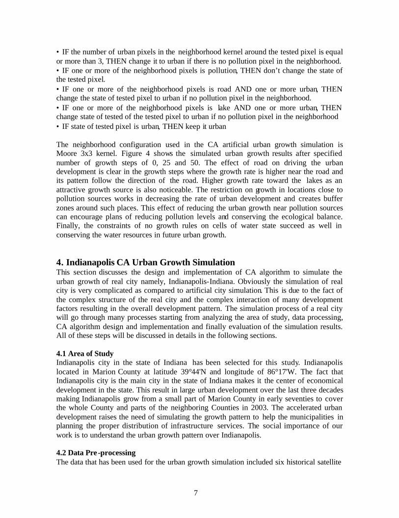
• IF the number of urban pixels in the neighborhood kernel around the tested pixel is equal or more than 3, THEN change it to urban if there is no pollution pixel in the neighborhood. • IF one or more of the neighborhood pixels is pollution, THEN don’t change the state of the tested pixel. • IF one or more of the neighborhood pixels is road AND one or more urban, THEN change the state of tested pixel to urban if no pollution pixel in the neighborhood. • IF one or more of the neighborhood pixels is lake AND one or more urban, THEN change state of tested of the tested pixel to urban if no pollution pixel in the neighborhood • IF state of tested pixel is urban, THEN keep it urban The neighborhood configuration used in the CA artificial urban growth simulation is Moore 3x3 kernel. Figure 4 shows the simulated urban growth results after specified number of growth steps of 0, 25 and 50. The effect of road on driving the urban development is clear in the growth steps where the growth rate is higher near the road and its pattern follow the direction of the road. Higher growth rate toward the lakes as an attractive growth source is also noticeable. The restriction on growth in locations close to pollution sources works in decreasing the rate of urban development and creates buffer zones around such places. This effect of reducing the urban growth near pollution sources can encourage plans of reducing pollution levels and conserving the ecological balance. Finally, the constraints of no growth rules on cells of water state succeed as well in conserving the water resources in future urban growth. 4. Indianapolis CA Urban Growth Simulation This section discusses the design and implementation of CA algorithm to simulate the urban growth of real city namely, Indianapolis-Indiana. Obviously the simulation of real city is very complicated as compared to artificial city simulation. This is due to the fact of the complex structure of the real city and the complex interaction of many development factors resulting in the overall development pattern. The simulation process of a real city will go through many processes starting from analyzing the area of study, data processing, CA algorithm design and implementation and finally evaluation of the simulation results. All of these steps will be discussed in details in the following sections. 4.1 Area of Study Indianapolis city in the state of Indiana has been selected for this study. Indianapolis located in Marion County at latitude 39°44'N and longitude of 86°17'W. The fact that Indianapolis city is the main city in the state of Indiana makes it the center of economical development in the state. This result in large urban development over the last three decades making Indianapolis grow from a small part of Marion County in early seventies to cover the whole County and parts of the neighboring Counties in 2003. The accelerated urban development raises the need of simulating the growth pattern to help the municipalities in planning the proper distribution of infrastructure services. The social importance of our work is to understand the urban growth pattern over Indianapolis. 4.2 Data Pre-processing The data that has been used for the urban growth simulation included six historical satellite

8

images cover Marion County covering a period of thirty years. These raw images include one 60 m resolution MSS image (1973) and four 30 m resolution TM images (1982, 1987, 1993 and 2003). The images are geometrically rectified to the same projection of Universal Transverse Mercator (UTM) NAD1983 zone 16N. Projected images are registered to spatially fit over each other using a second order polynomial transformation function and 12 well defined control points. Registration errors are very small represented by values far less than one pixel. 4.3 Images Classification After the images were geometrically rectified and registered spatially to each other, the next step to prepare the images as inputs to the CA simulation algorithm is image classification. Seven classes are defined based on Anderson classification system (1976): water, road, commercial, forest area, residential areas, pasture and row crops. Commercial and residential classes will be combined after the simulation as one class called urban. Ground reference data sources including orthophotographs, old aerial photographs and Indiana Geologic Survey (IGS) classification maps are used for identifying the land cover classes and for training and testing data collection. Maximum likelihood classification method is used for supervised classification. Classification accuracy report is prepared for each classified image using the testing data to check the quality of classification. Results indicate high accuracy level of classification above 85%. 4.4 CA Algorithm Toolkit Design in ArcGIS In this section we will discuss the detailed process of design and implementation of CA algorithm in ArcGIS 9.0 programming environment to simulate the urban growth in Indianapolis over thirty years. The first stage in the designing of CA urban growth simulation tool in ArcGIS is creating a new toolbar through customization process in ArcGIS. The second stage includes the definition of CA growth rules that is tuned after evaluating the simulation results. The following rules are identified to drive the growth through the CA algorithm in the same sequence presented: 1. IF tested pixel under consideration is water, THEN no growth is allowed at this pixel. 2. IF tested pixel under consideration is road, THEN no growth is allowed at this pixel. 3. IF tested pixel under consideration is residential OR commercial, THEN keep this pixel

the same without any change. 4. IF tested pixel under consideration is either (forest OR pasture OR row crops) AND

there are 4 commercial pixels in the neighborhood, THEN change tested pixel to commercial.

5. IF tested pixel under consideration is either (forest OR pasture OR row crops) AND there are 4 residential pixels in the neighborhood, THEN change tested pixel to residential.

Rules 4 and 5 are the tuned optimized versions of CA rules that provide the minimum error when comparing the simulated results and the ground truth. Commercial and residential classes are used separately in the simulation but they will be merged at the end of simulation in one class (Urban) for the evaluation and validation purposes.

9

Figure 4. Constrained CA artificial city urban growth simulation

In stage three of the CA simulation process, the oldest classified image 1973 is selected as an input for CA urban simulation. For each growth simulation step, a new empty achromatic raster image with the same size as the input classified image (1973) of 1457*1194 pixels is created. This image is populated by the updated pixel values after implementing CA crisp rules defined in stage two at each step. A 3x3 Moore neighborhood is used in the simulation process. The updated center pixel is determined as a function of current state of center pixel and the states of the neighborhood pixels. The output image of one growth step is used as input for the next growth step to have accumulative urban

10

growth. The fourth stage is converting the simulated CA image back to the color ramp of original input classified image for better visualization. A 2-D array is created to store the defined output raster image color ramp through defining the unique RGB codes for each color in the image. Ground truth images 1982 and 1993 are used for training to calibrate the CA rules and growth step while ground truth images of 1987 and 2003 are used for testing purposes only. The simulated CA image for the first ground truth (1982) is obtained after running the CA algorithm using different scenarios of CA rules and growth steps to accumulate the growth to this date. Growth step and CA rules are calibrated through testing the scenarios results’ by comparing them to the ground truth of image 1982 and select the growth step and CA rule with minimum simulation error. Once the calibrated step and CA rules are obtained, they are used to run the simulation to predict the growth for year 1987. Ground truth image 1993 is used as well to calibrate the CA rules and growth step based on which the 2003 growth is predicted. The fifth stage includes the design of an evaluation tool to evaluate the accuracy of simulation as compared to the ground truth to update the growth rules sand steps for minimizing the simulation uncertainty. An area of interest that covers Indianapolis of size (600x860) pixels or (36x51.6) kilometres selected from the image is used for evaluation. Selected area of the image is divided into 9 regions to evaluate the simulation results on region basis that take into account the spatial distribution of urban development. Figure 5 presents the index of dividing the study area into regions : North West (NW), North (N), North East (NE), West (W), Central, East (E), South West (SW), South (S) and South East (SE). A 2-D array is created with the same size of whole image. The simulated image is scanned on region basis pixel by pixel. Each pixel is identified to which class and region it belongs and saved in the reserved part of the array. The output is exported as a text file table with rows represent the region numbers and columns represent ing the land use type. The application of the designed evaluation tool appears in two main aspects: 1. Through scanning the ground truth images of the years 1973, 1982, 1987, 1993 and 2003, the total urban pixels (residential & commercial) are determined per image. This data is used to identify the real urban growth relationship for Indianapolis over 30 years. Also, the simulated images based on best growth scenario are scanned for comparison. The numerical results for both the ground truth and simulated images are shown in Table 1. The best scenarios adopted to simulate the Indianapolis urban growth will be discussed in details in next section. Figure 6 shows the graphical urban growth relation for both real vs. simulated results. The growth relations presented in Figure 6 can be estimated with exponential formulas for both real and simulated growth results presented in Equations 7 and 8 respectively.

0.0239xy = 156850e (7)

0.0217xy = 151538e (8)

11

where; y is the # of urban growth pixels and x is the time interval referenced to 1973.

Figure 5. Division of image study area for evaluation

Table 1. Indianapolis urban growth from ground truth and simulated images

Year Delta years # of Urban pixels for Ground truth

# of Urban pixels for Simulated images

1973 0 144736 151538 1982 9 209833 187829 1987 14 227812 191926 1993 20 258545 264167 2003 30 304478 275329

In both exponential formulas the exponential relations fit the data very well with a high coefficient of determination 2R of 0.9449 for ground truth data and 0.9131 for the simulated results. The results presented in Equations 7 and 8, Table 1 and Figure 6 indicate how the simulation results closely match with the ground truth. The two growth relationships present very close trend of urban growth over 3 decades in Indianapolis. The urban growth data at 1973 is used only as input image to initiate the simulation. A sharp increase in the growth at the end of eighties and early nineties can be seen in the urban growth patterns through the higher slope at this period. This might give an indication as we will see later that rules might need to be tuned in this period to adapt such jump in the urban growth for more realistic simulation. 2. The second important use of the designed evaluation tool is to compare the number of pixels for urban class of the ground truth images with CA simulation results. The result of this evaluation will produce the uncertainty in our simulation that will result in a feedback to tune the CA parameters for more accurate results. 5. Results and Discussion This section will implement the designated CA-GIS simulation tool on Indianapolis oldest

12

0

50000

100000

150000

200000

250000

300000

350000

0 5 10 15 20 25 30 35Year interval measured from 1973

# o

f u

rban

pix

els

urban pixels number forground truth

urban pixels number forsimulated images

Expon. (urban pixels numberfor ground truth)

Expon. (urban pixels numberfor simulated images)

Figure 6. Indianapolis urban growth pattern from ground truth and CA simulation

classified image of 1973 to simulate the urban growth over thirty years. The classified 1973 image is used as the input image to start the simulation process. Simulation is carried out from 1973 to 1982 (ground truth image). 1982 simulated image is compared to 1982 ground truth through using the evaluation tool. The error between the simulated and ground truth image is used to tune the CA rules and to calibrate the growth step of urban growth simulation. According to the results of many scenarios of defining the CA rules to minimize the simulation error, the growth step is best calibrated to correspond to one growth year. Using the result that the completion of each step of CA growth is calibrated to represent 1 growth year, CA rules defined in stage 2 are used except changing rules 4 and 5 to minimize the error of simulation. Many scenarios are tested to tune the CA rules 4 and 5. We will only mention here the best two scenarios used for rules 4 and 5 to run the simulation from 1973 to 1982 for the updated rules: Scenario 1: Rule 4: IF center pixel under consideration is either (forest OR pasture OR row crops) AND there are 4 commercial pixels in the neighborhood, THEN change center pixel to commercial. Rule 5: IF center pixel under consideration is either (forest OR pasture OR row crops) AND there are 3 residential pixels in the neighborhood, THEN change center pixel to residential. The CA simulation is run from 1973 to 1982 based on these rules for 9 calibrated growth steps. The simulated image is evaluated and compared to the 1982 ground truth image to

13

have feedback for updating the rules. Table 2 summarizes the comparison between simulated and ground truth of 1982 images for scenario 1.

Table 2. Scenario 1 CA simulation evaluation results of year 1982

Region

1982 Ground Truth (Urban1)

1982 simulated Urban

Error2

(pixels) Accuracy3 (%)

NW 12777 16957 4180 67.28 N 18686 27347 8661 53.65 NE 14740 22869 8129 44.85 W 26946 34412 7466 72.29 Central 39862 46952 7090 82.21 E 21639 32098 10459 51.67 SW 23580 24084 504 97.86 S 35131 34210 -921 97.38 SE 16472 19893 3421 79.23 Average accuracy for all zones 71.83

1Urban= (Commercial + Residential) 2Error (pixels) = (#Urban_simulated) - (#Urban_real) 3 Accuracy (%) = 100- abs (

(#Urban_simulated) - (#Urban_real)

(#Urban_real) * 100%)

Scenario 2: Rule 4: IF center pixel under consideration is either (forest OR pasture OR row crops) AND there are 4 commercial pixels in the neighborhood, THEN change center pixel to commercial. Rule 5: IF center pixel under consideration is either (forest OR pasture OR row crops) AND there are 4 residential pixels in the neighborhood, THEN change center pixel to residential. Table 3 evaluates the results of scenario 2. The evaluation results show more accurate simulation results using scenario 2. Results from Scenario 2 show higher average accuracy for all regions beside the higher accuracy achieved for simulation per region. Average accuracy of 90.21% for scenario 2 simulation versus 71.83% for scenario 1 is achieved. Due to the good results achieved by scenario 2, we decided to go with scenario 2 to simulate the growth from 1973 to the year 1982. Scenario 2 is used as well to continue the simulation to predict growth for year 1987 based on the same rules. Table 4 summarizes the urban growth prediction evaluation results based on scenario 2 for year 1987. The average simulation accuracy for year 1987 based on scenario 2 is 83.58%. High accuracy levels achieved as well for simulated regions ranging between 72.59% for West region to 96.49% for North West region. Urban growth simulation showed very promising results of simulating the urban growth of Indianapolis from 1973 to 1987 based on the best scenario adopted.

14


Region

1982 Ground Truth (Urban)


Error (pixels)

Accuracy (%)

NW 12777 12097 -680 94.68 N 18686 15811 -2875 84.61 NE 14740 14754 14 99.90 W 26946 23415 -3531 86.90 Central 39862 40021 159 99.60 E 21639 20391 -1248 94.23 SW 23580 18684 -4896 79.24 S 35131 26742 -8389 76.12 SE 16472 15914 -558 96.61 Average accuracy for all zones 90.21


Region



Error (pixels)

Accuracy (%)

NW 11884 12301 417 96.49 N 21175 16155 -5020 76.29 NE 15300 14996 -304 98.01 W 33034 23980 -9054 72.59 Central 46720 40875 -5845 87.49 E 25396 20686 -4710 81.45 SW 24614 18962 -5652 77.04 S 35428 27574 -7854 77.83 SE 14261 16397 2136 85.02 Average accuracy for all zones 83.58

Due to the growth jump observed before in the urban growth curve in late eighties and early nineties, the rules need to be modified to adapt such growth increase. This is achieved by relaxing the rules at this period as compared to continue growth using scenario 2. Numbers of scenarios are tested to select the best growth rules that take into account the growth jump. Best scenario selected after comparing the results of simulated 1993 image with the 1993 ground truth of modified version of rules 4 and 5 as follows: Rule 4: IF center pixel under consideration is either (forest OR pasture OR row crops) AND there are 3 residential pixels in the neighborhood, THEN change center pixel to residential. Rule 5: IF center pixel under consideration is either (forest OR pasture OR row crops) AND there are 4 commercial pixels in the neighborhood, THEN change center pixel to commercial. The modified rules are used to simulate the cumulative urban growth from 1987 to 1993. Table 5 presents the evaluated results of 1993 urban growth simulation. Average accuracy for the simulation of 1993 is 92.85%. The accuracy of all regions is also promising with a

15

range of accuracies between 72.95% for Central region to 99.54% for West region. Modified rules used to simulate 1993 are adopted again to drive the urban growth from 1993 up to predict 2003 with 10 calibrated growth steps in a long term prediction manner. The evaluation results of predicted 2003 growth are shown in Table 6.

Table 5. CA simulation evaluation results of year 1993

Table 6. CA simulation evaluation results of year 2003

The average accuracy achieved for the predicted year 2003 of 85.65% is encouraging especially for such long term prediction of 10 years interval. The simulated CA urban growth images for the years 1982, 1987, 1993 and 2003 versus ground truth images are presented in Figures 7 to 10 respectively. Visual comparison of simulated and ground truth images shows close visual match between the two urban growth spatial distribution patterns. Urban distribution in ground truth as compared to the simulated ones show spatial match all over the image area of study. Excessive urban growth rate took place over Indianapolis in the last thirty years as can be noticed in the simulated images. Based on the CA simulation strategy we used to predict 2003, future prediction of Indianapolis urban growth can be simulated. Such prediction will help municipalities identify the future growth trend and design the sustainable infrastructure plans to accommodate such trend.

Region



Error (pixels)

Accuracy (%)

NW 21997 22448 451 97.95 N 27794 26027 -1767 93.64 NE 23797 24079 282 98.81 W 32519 32370 -149 99.54 Central 36512 46389 9877 72.95 E 28535 29567 1032 96.38 SW 27273 24632 -2641 90.32 S 36326 33434 -2892 92.04 SE 23792 25221 1429 93.99 Average accuracy for all zones 92.85

Region



Error (pixels)

Accuracy (%)

NW 18212 27758 9546 47.58 N 33466 33482 16 99.95 NE 28785 30376 1591 94.47 W 39383 38296 -1087 97.24 Central 46990 47672 682 98.55 E 36621 37914 1293 96.47 SW 32816 27256 -5560 83.06 S 45161 35812 -9349 79.3 SE 23044 28977 5933 74.25 Average accuracy for all zones 85.65

16

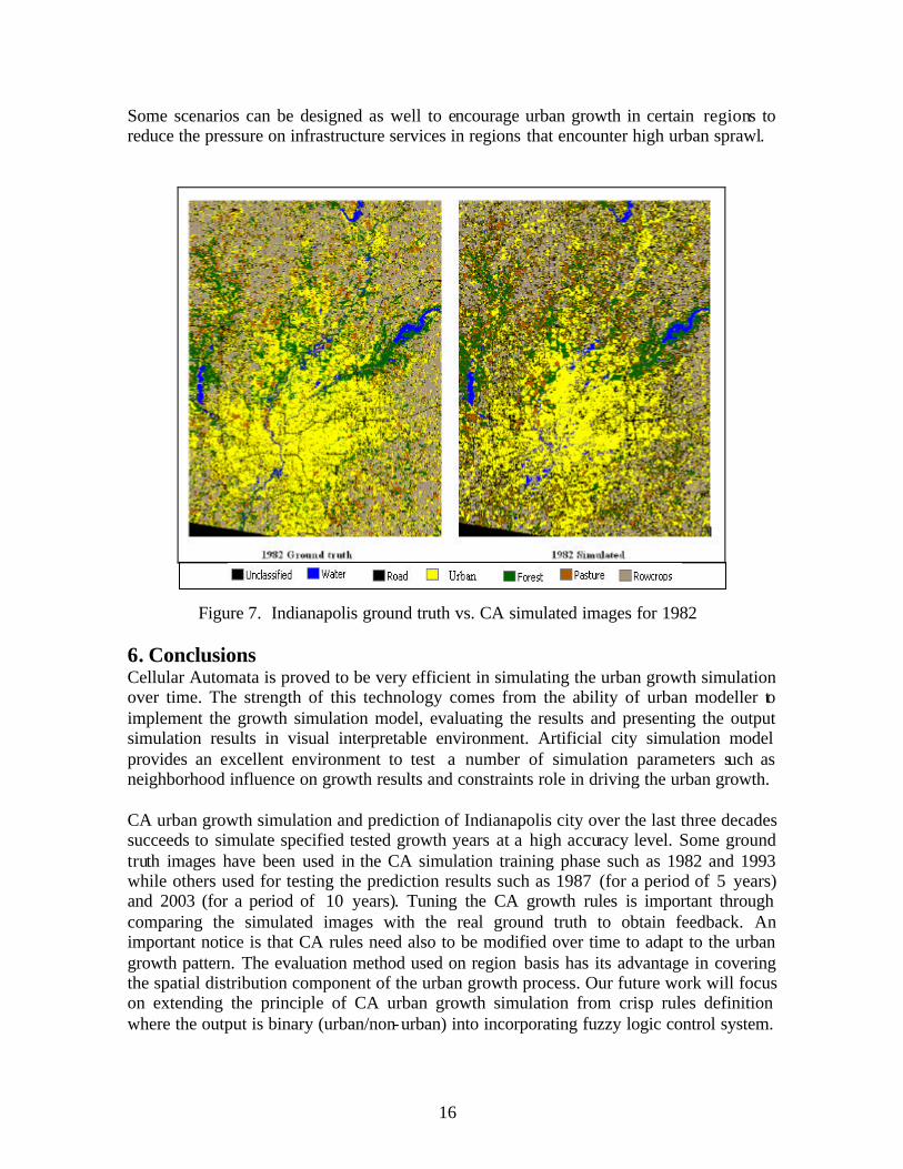
Some scenarios can be designed as well to encourage urban growth in certain regions to reduce the pressure on infrastructure services in regions that encounter high urban sprawl.

Figure 7. Indianapolis ground truth vs. CA simulated images for 1982

6. Conclusions Cellular Automata is proved to be very efficient in simulating the urban growth simulation over time. The strength of this technology comes from the ability of urban modeller to implement the growth simulation model, evaluating the results and presenting the output simulation results in visual interpretable environment. Artificial city simulation model provides an excellent environment to test a number of simulation parameters such as neighborhood influence on growth results and constraints role in driving the urban growth.

CA urban growth simulation and prediction of Indianapolis city over the last three decades succeeds to simulate specified tested growth years at a high accuracy level. Some ground truth images have been used in the CA simulation training phase such as 1982 and 1993 while others used for testing the prediction results such as 1987 (for a period of 5 years) and 2003 (for a period of 10 years). Tuning the CA growth rules is important through comparing the simulated images with the real ground truth to obtain feedback. An important notice is that CA rules need also to be modified over time to adapt to the urban growth pattern. The evaluation method used on region basis has its advantage in covering the spatial distribution component of the urban growth process. Our future work will focus on extending the principle of CA urban growth simulation from crisp rules definition where the output is binary (urban/non-urban) into incorporating fuzzy logic control system.

17



18


7. References Anderson, J. R., Hardy, E. E., Roach, J. T., and Witmer, R. E., 1976, A land use and land

cover classification system for use with remote sensor data. USGS Professional Paper 964, Sioux Falls, SD, USA.

Batty, M., and Xie, Y., 1994a, From cells to cities. Environment and Planning, B21, 531-548.

Batty, M., and Xie, Y., 1994b, Modelling inside GIS: Part 2. Selecting and calibrating urban models using ARC-INFO. International Journal of Geographical Information Systems, 8, 451-470.

Batty, M., 1998, Urban evolution on the desktop: simulation with the use of extended cellular automata. Environment and Planning A, 30, 1943-1967.

Batty, M., Xie, Y., and Sun, Z., 1999, Modeling urban dynamics through GIS-based cellular automata. Computers, Environment and Urban Systems, 23, 205-233.

Clarke, K. C., Hoppen, S., and Gaydos, L., 1997, A self-modifying cellular automaton model of historical urbanization in the San Francisco Bay area. Environment and planning B, 24, 247-261.

Codd, E. F., 1968, Cellular Automata. Academic Press, New York. Li, X., and Yeh, A.G.O., 2000, Modelling sustainable urban development by the

integration of constrained cellular automata and GIS. International Journal of Geographical Information Science, 14, 131-152.

Meaille, R., and Wald, L., 1990, Using geographical information systems and satellite imagery within a numerical simulation of regional urban growth. International Journal of Geographic Information Systems, 4, 445-456.

19

Pijanowski, B. C., Long, D. T., Gage, S. H., and Cooper, W. E., 1997, A land transformation model: conceptual elements, spatial object class hierarchies, GIS command syntax and an application for Michigan’s Saginaw Bay Watershed. http://www.ncgia.ucsb.edu/conf/landuse97/ papers/ pijanowski_bryan/paper.html.

Sipper, M., 1997, Evolution of Parallel Cellular Machines: The Cellular Programming Approach. 3-8, Springer-Verlag, Heidelberg.

Tsoukalas, L. H., and Uhrig, R. E., 1997. Fuzzy and Neural Approaches in Engineering. 189-289 and 385-405, John Wiley and Sons, New York.

Turner, M. G., 1987, Spatial simulation of landscape changes in Georgia: A comparison of 3 transition models. Landscape Ecology, 1, 29-36.

Veldkamp, A., and Fresco, L. O., 1996, CLUE: A conceptual model to study the conversion of land use and its effects. Ecological Modelling, 85, 253-270.

von Neumann, J., 1966, Theory of Self-Reproducing Automata. University of Illinois Press, Illinois. Edited and completed by A. W. Burks.

White, R., and Engelen, G., 1997, Cellular automata as the basis of integrated dynamic regional modelling. Environment and Planning B, 24, 235-246.

Wu, F., and Webster, C. J., 1998, Simulation of land development through the int egration of cellular automata and multi-criteria evaluation. Environment and Planning B, 25, 103-126

Wu, F., 2002, Calibration of stochastic cellular automata: the application to rural-urban land conversions. International Journal of Geographical Information Science, 16, 795-818.

Yang, X., and Lo, C. P., 2003, Modelling urban growth and landscape changes in the Atlanta metropolitan area. International Journal of Geographical Information Science, 17, 463-488.

cellular automata urban growth simulation and …jshan/publications/2005/geocompute...ground truth...

Documents