MPP-2018-20

Infinite Distances in Field Space and Massless Towers of States

Thomas W. Grimm1, Eran Palti2, Irene Valenzuela1

1 Institute for Theoretical Physics

Utrecht University, Princetonplein 5, 3584 CE Utrecht, The Netherlands

2Max-Planck-Institut fur Physik (Werner-Heisenberg-Institut),

Fohringer Ring 6, 80805 Munchen, Germany

Abstract

It has been conjectured that in theories consistent with quantum gravity infinite distances infield space coincide with an infinite tower of states becoming massless exponentially fast inthe proper field distance. The complex-structure moduli space of Calabi-Yau manifolds is agood testing ground for this conjecture since it is known to encode quantum gravity physics.We study infinite distances in this setting and present new evidence for the above conjecture.Points in moduli space which are at infinite proper distance along any path are characterisedby an infinite order monodromy matrix. We utilise the nilpotent orbit theorem to show thatfor a large class of such points the monodromy matrix generates an infinite orbit within thespectrum of BPS states. We identify an infinite tower of states with this orbit. Further,the theorem gives the local metric on the moduli space which can be used to show thatthe mass of the states decreases exponentially fast upon approaching the point. We alsopropose a reason for why infinite distances are related to infinite towers of states. Specifically,we present evidence that the infinite distance itself is an emergent quantum phenomenoninduced by integrating out at one-loop the states that become massless. Concretely, weshow that the behaviour of the field space metric upon approaching infinite distance canbe recovered from integrating out the BPS states. Similarly, at infinite distance the gaugecouplings of closed-string Abelian gauge symmetries vanish in a way which can be matchedonto integrating out the infinite tower of charged BPS states. This presents evidence towardsthe idea that also the gauge theory weak-coupling limit can be thought of as emergent.

arX

iv:1

802.

0826

4v2

[he

p-th

] 2

3 M

ar 2

018

Contents

1 Introduction 2

2 Infinite distance divisors in Calabi-Yau moduli space 5

2.1 Complex structure moduli space and monodromy . . . . . . . . . . . . . . . . . . 5

2.2 The local Kahler potential and a necessary condition for infinite distance . . . . 7

2.3 Infinite distance paths in one-parameter degenerations . . . . . . . . . . . . . . . 10

3 Massless BPS States 11

3.1 Monodromy orbits and massless states . . . . . . . . . . . . . . . . . . . . . . . . 13

3.2 The monodromy orbit and BPS states . . . . . . . . . . . . . . . . . . . . . . . . 17

3.3 The exponential mass behaviour . . . . . . . . . . . . . . . . . . . . . . . . . . . 21

3.4 Microscopic physics for BPS stability . . . . . . . . . . . . . . . . . . . . . . . . . 23

4 Infinite monodromy orbits and mixed Hodge structures 25

4.1 A coarse introduction to the refined Hodge structure . . . . . . . . . . . . . . . . 25

4.2 Mathematical machinery of mixed Hodge structures . . . . . . . . . . . . . . . . 27

4.3 Infinite monodromy orbits at singular loci . . . . . . . . . . . . . . . . . . . . . . 34

4.4 Monodromy intersection loci . . . . . . . . . . . . . . . . . . . . . . . . . . . . . . 39

5 Infinite distances from integrating out states 42

5.1 Field space corrections from integrating out states . . . . . . . . . . . . . . . . . 43

5.2 Application to the monodromy loci . . . . . . . . . . . . . . . . . . . . . . . . . . 46

5.3 Relation to the Scalar WGC and to global symmetries . . . . . . . . . . . . . . . 48

6 The gauge kinetic function and the Weak Gravity Conjecture 50

6.1 Behaviour of the gauge kinetic function . . . . . . . . . . . . . . . . . . . . . . . 50

6.2 Gauge kinetic function from integrating out states . . . . . . . . . . . . . . . . . 52

7 Summary 55

A Non-mutually stable BPS states 59

B Some simple examples and classification results 60

1

1 Introduction

Quantum field theory and gravity are notoriously difficult to combine at high energy scales close

to the Planck mass Mp. However, at low energies, there might appear to be no consistency

constraints limiting which effective quantum field theories can be coupled to gravity.1 This

apparent freedom is deeply tied to the difficulty of obtaining universal predictions from string

theory. In recent years there has been significant interest in proposals for such consistency

constraints on effective field theories that can be coupled to quantum gravity. Quantum field

theories which violate such constraints are termed to be in the Swampland [1]. The most studied

such proposed constraint is the Weak Gravity Conjecture [2]. A different constraint, proposed

in [3], is that in an effective quantum field theory that can can arise from string theory and

therefore can be consistently coupled to quantum gravity, infinite distances in moduli space lead

to an infinite tower of states becoming massless exponentially fast in the proper field distance.

So if we consider two points in field space P and Q, with a geodesic proper distance between

them of d (P,Q), then there should exist an infinite tower of states with characteristic mass

scale m such thatm (P )

m (Q)→ e−γd(P,Q) as d (P,Q)→∞ . (1.1)

Here γ is some positive constant which depends on the choice of P and Q but which is not

specified in generality. The conjecture (1.1) was referred to as the Swampland Conjecture in [4].

Since there are more conjectures appearing recently to distinguish between the string landscape

and the swampland, here we will rename this specific conjecture as the Swampland Distance

Conjecture (SDC) to avoid confusion. This conjecture will form the focus of this paper. One

of the consequences of the conjecture is a limit on moduli space distances within any effective

field theory which is consistent with string theory and has a finite cut-off. It is therefore of both

formal and conceptual interest and of potential phenomenological importance in the context of

large field inflation.

The evidence for the conjecture is primarily based on case-by-case examples in string theory.

There is some evidence, which does not rely on string theory, relating the Swampland Distance

Conjecture to the Weak Gravity Conjecture [5] and to black hole physics [4]. It is also worth

noting that the evidence appears to support a stronger statement, that the exponential behaviour

of the mass of the states is reached at finite proper distance of order the Planck mass and that it

holds for any scalar field not just moduli. This was denoted as the Refined Swampland (Distance)

Conjecture in [4]. In [6,7] the behaviour of so-called closed-string monodromy axions in type

IIA string theory was shown to be consistent with this stronger statement. Further evidence for

the conjecture was found in [8–10] in the context of studying open-string monodromy axions,

although the breakdown of the effective theory there manifests in a more subtle way. In [5] the

Swampland Distance Conjecture was shown to hold for string moduli in the large volume or

large complex-structure regime of Calabi-Yau compactifications for certain paths in moduli space

defined by the variation of only a linear combination of the moduli. In [11] further evidence was

presented in the context of closed string axions belonging to the complex structure sector of

certain Type IIB string theory flux compactifications. In [12] a similar bound was found for

the reduced Kahler moduli space obtained from Type IIB compactified on a certain type of

Calabi-Yau threefolds. Further studies, over the full complex-structure moduli space of type IIB

Calabi-Yau compactifications, will be reported in [13].

1Mixed gauge-gravitational anomalies providing a notable exception.

2

In this paper we will adopt a general approach to studying the Swampland Distance

Conjecture where we do not rely on explicit example compactifications but rather on general

properties of a large and rich class of moduli spaces in string theory. We will consider the

complex-structure moduli spaces of Calabi-Yau (CY) manifolds in compactifications of type IIB

string theory. These moduli spaces are excellent testing grounds for aspects of quantum gravity

as they are known to encode highly non-trivial quantum gravity physics in their geometry. A

CY complex-structure moduli space also has a very rich structure of loci that are at infinite

distance. By this we mean points in the moduli space which are at infinite proper distance,

as measured by the metric on the moduli space, along any path. There are also substantial

mathematical tools for studying these moduli spaces which will allow us to show general results

rather than a case-by-case analysis.

Furthermore, most of the recent work has been focused on the parametric behaviour of the

field metric, but very little is known about the nature of the tower of states becoming light.

We will also focus on studying the properties of this tower of states, providing a candidate set

of stable states which become massless at infinite distances. Specifically, we will consider the

tower to be formed of BPS states, which in type IIB are D3-branes wrapping special Lagrangian

three-cycles. Once this tower is identified, we will show that the exponential mass behaviour of

the Swampland Distance Conjecture can be proven in generality due to a powerful mathematical

theorem, termed the Nilpotent Orbit Theorem [14], which, among other things, gives a general

expression for the asymptotic infinite distance form of the field space metric. Identifying the

tower requires an understanding of the BPS state spectrum upon approaching infinite distance.

The infinite distance point is singular and there is a monodromy upon circling it. It can be

mathematically proven that this monodromy must be of infinite order. We will propose to identify

an infinite tower of states by using the monodromy transformation acting on the states of the

theory upon circling the infinite distance locus. By introducing significant further mathematical

technology, particularly relating to Mixed Hodge Structures, we will be able to identify this

tower quite precisely. Our analysis will be performed completely generally, for any CY moduli

space and at any point in that moduli space. But we will restrict to one-parameter degeneration

models, which means that the point of interest will belong to only one singular divisor, leaving

more complicated configurations for future work. Because these are rich field spaces, possibly

involving hundreds of coupled scalar fields, the analysis necessitates powerful mathematical

machinery. A significant part of the paper will therefore be dedicated to introducing these tools

and how they can be used in this context.

Our results can be summarised as follows. A locus of infinite distance in moduli space is

labelled by an integer d which can take the values 1, 2 or 3. For d = 3 loci we will identify

quite precisely and generally a tower of BPS states which become massless exponentially fast in

the proper distance. This is one of the central results of the paper. For d < 3 loci we will also

propose candidates for the tower of BPS states. However, proving the existence of this tower can

not be done with the same generality as for d = 3 due to dependence on the global structure of

the moduli space. Studying the generality of the results for such cases will require further work.

We will also provide evidence for a proposal for the underlying reason as to why the

Swampland Distance Conjecture holds. We will show that integrating out the tower of BPS

states induces a logarithmic distance divergence in the moduli space. Since it is well known that

CY moduli spaces are quantum in nature, so that they already have integrated out the BPS

states of wrapped branes, this divergence is naturally identified with the infinite distance in

3

the moduli space. We therefore propose that this could be a general phenomenon, that infinite

distances are quantum in nature and emerge from integrating out an infinite number of states.2

Interestingly, the logarithmic divergence in the proper field distance requires that the number of

stable BPS states grows as we approach the singularity, becoming infinite at infinite distance.

By studying the distribution of walls of marginal stability for BPS states, we will show that the

tower of states induced by the monodromy transformation exhibits precisely the right rate of

increase in the stable states to match onto the integrating out requirements. It also implies that

the cut-off due to quantum gravity physics decreases when we approach the singularity at a rate

which coincides with the species bound relating to the tower of BPS states.

Our results also have natural interpretations relating to other general ideas about quantum

gravity. We will show in generality that infinite distances are loci in field space where a global

symmetry emerges. Since the effective theory entirely breaks down at the infinite distance

singularities, the emergence of these global symmetries is blocked by string theory.

Because the complex-structure moduli are in vector multiplets our results have a natural

connection to the Weak Gravity Conjecture. We will show that at infinite distance the gauge

couplings of the Abelian gauge fields in the vector multiplets vanish exponentially fast in the

proper distance. This matches the proposal in [4]. We will show that this behaviour can be

recovered in detail in terms of integrating out a tower of charged BPS states. It therefore

presents evidence that also the weak coupling limit is emergent in the same way as the infinite

field distance. This emergence property will naturally tie into the Weak Gravity Conjecture.

This matches general ideas proposed in [16].

The paper is organised as follows. In section 2 we introduce the mathematical technology

required to analyse infinite distance points in the moduli space of Calabi-Yau manifolds. We will

introduce the Nilpotent Orbit Theorem of Schmid [14] and how it can be used to characterise

infinite distance loci and study them generally. In particular, we will introduce the relation

between infinite distance loci and infinite order monodromy transformations about those loci.

In section 3 we will introduce some relevant results about BPS states. We will discuss the

relation between the monodromy transformation and the spectrum of BPS states. In particular,

we will introduce the notion of an infinite monodromy orbit of massless BPS states, and show

that this orbit forms a primary candidate for a subset of the spectrum of states which become

massless on the monodromy locus. In section 4 we will introduce the technology of Mixed

Hodge Structures and their utilisation in the Sl2-orbit theorem of Schimd [14]. This will then

allow us to study when an infinite monodromy orbit through massless BPS states exists and to

identify it quite precisely. We will present general results on this, and also study some particular

examples. In sections 5 and 6 we will discuss some of the physics associated to our results.

In particular, the relation between integrating out states, infinite distances, gauge couplings

and global symmetries, as described above. We will also discuss the relation of the Swampland

Distance Conjecture to the Weak Gravity Conjecture and the idea that they are both implied

by the emergent nature of infinite field distance and weak gauge couplings. Finally, section 7

contains our conclusions.

2This possibility was first mentioned in [3], and also a similar proposal was reached independently in [15].

4

2 Infinite distance divisors in Calabi-Yau moduli space

In this section we introduce the mathematical concepts that allow us to study points in moduli

space that are at infinite geodesic distance with respect to some specific metric g. We denote a

point of infinite distance as one for which all paths γ to such a point are infinitely long when

measured with the metric g. Hence we want to make statements about the length of any smooth

path γ connecting P,Q given by

dγ(P,Q) =

∫γ

√gIJ xI xJds , (2.1)

where xI(s) embeds the path and xI = ∂xI/∂s. The key point will be to translate the information

about being at infinite distance into a more algebraic statement. Firstly, we note that infinite

geodesic distances can only occur when connecting a path to a singular point P in moduli space

as indicated in Figure 1. Secondly, we will see that such points are characterised by the existence

of an infinite order monodromy matrix T and by the action of the logarithm N = log(T ) of the

monodromy matrix acting on the unique holomorphic three-form at this point. This will allow

us to identify the universal asymptotic behaviour of the field metric g when approaching such

infinite distance points.

singular locus

P

Q

Figure 1: Smooth path connecting a regular point Q to a singular point P which might be atinfinite distance in moduli space.

2.1 Complex structure moduli space and monodromy

To start with we recall some basic facts about the complex structure moduli space Mcs and

introduce its natural metric, the Weil-Petersson metric gWP. The complex structure moduli

space for a Calabi-Yau manifold YD of complex dimension D is a hD−1,1(YD)-dimensional Kahler

manifold. Locally, it can be parametrised by coordinates zI , I = 1, . . . , hD−1,1(YD), which are

often called the complex structure deformation moduli. The metric on Mcs is determined by

the holomorphic (D, 0)-form Ω. The metric gWP is Kahler and locally obtained from the Kahler

potential [17, 18]

K = − log[− iD

∫YD

Ω ∧ Ω], (2.2)

i.e. one finds that gWP has components gIJ = ∂zI∂zJK.

The holomorphic (D, 0)-form Ω can be expanded into an appropriate real integral basis

γI . It is a non-trivial task to identify such an ‘appropriate’ integral basis γI . We refer to the

5

literature discussing Calabi-Yau threefold and fourfolds for more details on its construction.

Furthermore, one can show that Ω depends holomorphically on the coordinates zI . Hence, we

write

Ω = ΠI(z) γI ≡ ΠTγ , ΠI =

∫ΓI

Ω , (2.3)

where γI integrates to δJI over the cycle ΓJ . The holomorphic functions ΠI are called the

periods of Ω. In order to rewrite intersection products it will be also convenient to introduce

the intersection matrix η with components

ηIJ =

∫YD

γI ∧ γJ , (2.4)

which is anti-symmetric for D odd and symmetric for D even. In Calabi-Yau threefolds,

i.e. D = 3, the matrix ηIJ is anti-symmetric and the basis γI can be chosen to be symplectic.

Hence, we can pick

γI = (αL, βK) ,

∫Y3

αL ∧ βK = δKL ,

∫Y3

αL ∧ αK =

∫Y3

βL ∧ βK = 0 . (2.5)

Let us stress that the coordinates zI , periods Π(z)I , and the basis γI are adapted to the

considered patch in Mcs and can very non-trivially change when moving to different regions in

Mcs. With this definitions at hand we can write (2.2) as

K = − log[− iDΠT ηΠ

]. (2.6)

It is crucial for our considerations that the complex structure moduli space Mcs is not

generally smooth, but will admit special singular points. These can always be made to lie

on divisors that intersect normally.3 The periods Π are in fact multi-valued and experience

monodromies along paths encircling such special divisors. To make this more precise, let us

introduce local coordinates zI , such that the considered singular divisor is given by zj = 0 for

some j ∈ 1, . . . , hD,1(YD). Note that we can consider several intersecting divisors. We encircle

zj = 0 by sending zj → e2πizj . In general the periods will non-trivially transform with a matrix

Ti under this identification

Π(..., e2πizj , ...) = Tj Π(..., zj , ...) . (2.7)

Two facts about the Tj will be important for us in the next sections [14,20]

each Tj is quasi-unipotent : ∃mj , nj ∈ Z : (Tmj+1 − Id)nj+1 = 0 , (2.8)

Tj locally arising at a point commute : [Ti, Tj ] = 0 . (2.9)

Collecting all such Ti throughout the moduli space Mcs one obtains a group Γ known as the

monodromy group.4 In general, the elements of Γ will not commute, and (2.9) only holds for

the elements Ti at a point in a higher-dimensional moduli space. However, we will not need a

detailed global understanding of the moduli space and therefore restrict most of our discussion

to a local patch around such special points. It is important to note that the ‘infinite distance’

in the metric gWP will be picked up in such a local patch if the special point satisfied certain

criteria. This will be discussed in the next subsections.3To be mathematically more precise, it was shown [19] that one can resolve the moduli space such that all

special points are on divisors that intersect normally.4Strictly speaking the monodromy group can be defined by considering a certain representation T JI of π1(Mcs)

acting on the period vectors.

6

2.2 The local Kahler potential and a necessary condition for infinite distance

Our next goal is to find a local expression for the Kahler potential (2.6) near the special points

in moduli space with non-trivial monodromy matices Ti. In order to do that we again introduce

an appropriate set zI of local coordinates. We first split them into two types

zI = (zj , ζM ) , (2.10)

such that the special divisors are, as above, locally given by zj = 0. The complex coordinates

ζM will be included to keep the situation general. We will be interested in the point P given by

P : zj = 0, ζM = 0 , (2.11)

and expand the Kahler potential (2.6) around this point. By definition this point lies on the

special singular divisors zj = 0. Here ζM can take any value, so we have chosen ζM = 0 without

loss of generality.

The coordinates zj are not yet convenient for our purposes. The reason for this is that

part of the monodromy matrix Ti introduced when circling zj → e2πizj as in (2.7) will play no

important role when evaluating the distance. To identify this part, we note that the property

(2.8) implies that each Ti can be decomposed as

Ti = T(s)i · T

(u)i , (2.12)

with T(s)i and T

(u)i having the following special properties. Each matrix T

(s)i is of finite order,

i.e. there exists an integer mi such that (T(s)i )mi−1 6= Id and (T (s))mi = Id. In contrast, for each

matrix T(u)i is unipotent, i.e. T

(u)i is either the identity matrix or there exists an integer ni > 0

such that

(T(u)i − Id)ni 6= 0 , (T

(u)i − Id)ni+1 = 0 . (2.13)

If T(u)i is not the identity an unipotent matrix will be of infinite order, i.e. there exists no ki

such that T kii = Ti. This property will be of crucial importance below. The precise form of T(s)i

will not be relevant in the local expression of the Kahler potential. To avoid including factors of

mi all over the place we therefore redefine

zj → (zj)mj , (2.14)

but name, by an abuse of notation, the resulting coordinate zj .5 In terms of this new coordinate,

the monodromy matrix is only given by its infinite order part.

We are now ready to display the local form of the periods and the Kahler potential. To do

that we first define

Ni = log T(u)i =

∞∑k=1

(−1)k+1 1

k(T

(u)i − Id)k =

1

milog Tmii , (2.15)

which should be read as a matrix equation. One can easily check that the so-defined matrix Ni

is nilpotent with

Nnii 6= 0 , Nni+1

i = 0 , (2.16)

5In mathematical terms this transformation corresponds to a base change.

7

where ni was already introduced in (2.13). Using these nilpotent matrices it was shown by

Schmid [14] that locally around the point P given in (2.11) the periods take the form

Π(z, ζ) = exp[∑

j

1

2πi(log zj)Nj

]A(z, ζ) , (2.17)

with A being holomorphic at P . In other words, the non-trivial part of this statement is that a

crucial part of the information about the singularity is in the matrices Nj . The vector A(z, ζ)

is regular at P and admits an expansion

A(z, ζ) = a0(ζ) + aj(ζ)zj + ajk(ζ)zjzk + ajkl(ζ)zjzkzl + . . . (2.18)

The name ‘nilpotent orbit’ refers to the approximation exp[∑

j1

2πi(log zj)Nj

]a0(ζ) of the full

period Π(z, ζ).6

To display the Kahler potential we note that the monodromies Ti preserve η, i.e. T Ti ηTi = η,

and therefore one has

NTi η = −ηNi . (2.19)

Using this fact and the expansion (2.17) the Kahler potential (2.6) takes the form

e−K = −iDAT η exp[−∑j

1

2πi(log |zj |2)Nj

]A . (2.20)

To write this in a more practical form we define

tj =1

2πilog zj . (2.21)

Clearly, this redefinition implies that the point under consideration is now given by

P : tj = i∞, ζM = 0 . (2.22)

In these coordinates all t-dependence in A arises via exponentials e2πit. There are, however,

polynomial terms in t− t arising in e−K due to the exponential containing Ni. Inserting (2.21)

in (2.20) one finds

e−K = −iDAT η exp[∑

j

(tj − tj)Nj

]A (2.23)

= −iDaT0 η exp[∑

j

(tj − tj)Nj

]a0 +O(e2πit) , (2.24)

≡ p(Im ti, ζ) +O(e2πit) (2.25)

Due to the fact that the Nj are nilpotent, p is simply a polynomial in Im tj .

This form of the Kahler potential allows us to make a couple of important observations. We

note that near a singular point the Kahler potential K depends on Im tj through a polynomial

p as well as exponentially suppressed corrections O(e−Im tj ). In contrast, the coordinates Re ti

6Schmid gives an estimate how well this expression approximates the full period.

8

only appear in the exponentially suppressed terms in (2.25). This implies that if the degree of

the polynomial p is larger or equal to one in some variable Im tj then at large Im tj the Kahler

potential enjoys an approximate shift symmetry

Re tj → Re tj + cj , cj ∈ R , (2.26)

which is only broken by exponentially suppressed corrections to the discrete shifts with cj ∈ Z.

In physical terms one thus would identify Re tj as an axion. This agrees with the observation

made in [21] that axion in complex structure moduli space arise at special points that have

infinite order monodromy. Here we have shown this completely generally, by noting that Nj

only exists in these situations. Crucial is, however, that the polynomial has a non-vanishing

degree. To determine its degree we first introduce the integers di such that

Ndij a0 6= 0 , Ndi+1

j a0 = 0 . (2.27)

One might be tempted to assert that the degree of p in Im tj is simply dj , but this statement is

far from trivial since the degree could be lowered by a vanishing of the inner product involving

a0 and Nki a0. We will discuss in detail in subsection 2.3 (and prove it in section 4.2), that at

least for a one-dimensional degeneration the degree of the polynomial p is indeed d.

While it is hard to analyse infinite distance paths in the generality, it is possible to give a

rather simple necessary criterion when the point P is at infinite distance [22]. Since the complex

structure moduli space is Kahler, the length (2.1) of a path γ is measured by the integral

dγ(P,Q) =

∫γ

√2gIJ z

I ˙zJds , (2.28)

where gIJ is the Kahler metric derived from (2.25) evaluated along the path. The necessary

condition on dγ being infinite is

P at infinite distance ⇒ ∃Ni : Nia0 6= 0 . (2.29)

In other words, there has to be at least one monodromy Ti of infinite order that allows us

to define the Ni satisfying (2.29). Furthermore this infinite order Ti must act non-trivially

on a0. To show (2.29) it is easier to show the equivalent statement that if for all Ni one has

Nia0 = 0 then there is a path to the point which has a finite distance. So let us assume that

this latter statement is true. Then the Kahler potential (2.25) has no pure polynomial terms

in ti. Furthermore, one can use the tools presented in the next subsection to show that p is

constant in ti and does not vanish at P . Then one can focus on one specific path, namely the

path (ti(s), ζM (s)) = (is, ..., is, 0, ..., 0), and rather straightforwardly check that the integral

(2.28) is finite when integrating from s0 to ∞ [23]. Since there is at least one path to the point

which has finite distance, the point is said to be at finite distance in field space.

Let us end this section by pointing out that it is crucial to keep in mind that the arrow

in (2.29) points only in one direction. It was, however, conjectured in [23] that the opposite

direction is also true:

Conjecture: P at infinite distance ⇐⇒ ∃Ni : Nia0 6= 0 . (2.30)

The above sketch of a proof of (2.29) indicates why the other direction is much more involved.

In the proof one has to construct one path which has finite length, which then implies that the

9

point cannot be at infinite geodesic distance. Proving the opposite direction would require to

study features of all possible paths, which is enormously complicated since many non-trivial

cancellations can take place. In fact, this complication indicates a crucial problem that one is

facing whenever one tries to analyse field space distances: there are many possible paths and it

can be hard to disentangle features of a path from actual features of the metric.

In the next subsection we will see that in the case in which the point P lies on only a single

special divisor, we can supply the relevant mathematics and study the paths in more detail.

In fact, the conjecture (2.30) can then be proved and we will comment on the details of this

proof. The assumption of P being only on a single divisor reduces the problem to a complex

one-dimensional problem in which it becomes tractable.

2.3 Infinite distance paths in one-parameter degenerations

In the following we like to continue our study of infinite paths in the complex structure space

Mcs. In order to do this in detail we will impose restrictions on the points P we consider. Our

restriction will be that they only lie on a single special divisors. In this case we can study infinite

distance paths in detail and indicate how the conjecture (2.30) is proved.

In the considered special case, we can pick local complex coordinates (2.10) that are now

split as zI = (z, ζM ), in which the special singular divisor is locally given by z = 0. This local

coordinates are also chosen, such that the point of interest is put at the origin P : z = 0, ζM = 0.

Since we are dealing with a single divisor only, there is only a single monodromy matrix T

around z = 0, and a single nilpotent matrix N (2.15). Recall that N is given by

N = log T (u) =1

mlog Tm , (2.31)

where T (u) is the unipotent part of T . As above we perform a coordinate transformation z → zm

to remove factors of m and work only with T (u), N . For completeness, let us also display the

periods near P again

Π(z, ζ) = exp[ 1

2πi(log z)N

]A(z, ζ) , (2.32)

with

A(z, ζ) = a0(ζ) + a1(ζ)z + a2(ζ)z2 + a3(ζ)z3 + . . . , (2.33)

where the aj are holomorphic functions of ζM near P . In the coordinate t = 12πi log z this implies

that the Kahler potential takes the form

e−K = −iDaT0 η exp[− 2i Im tN

]a0 +O(e2πit, ζ) ≡ p(Im t, ζ) +O(e2πit, ζ) . (2.34)

The first term on the right is a polynomial in Im t and has again been denoted by p(Im t, ζ).

We are interested in the degree of the polynomial p. Therefore, as in (2.35), we first define

an integer d as

Nda0 6= 0 , Nd+1a0 = 0 , (2.35)

and note that since N is nilpotent with Nn+1 = 0 one has d ≤ n. Recall from (2.29) that if

d = 0 one has that the point P is at finite distance. We are interested, however, in infinite

10

distance points and therefore want to determine the degree of p in Im t. In order to do that, we

expand the exponential in p and write

p = −iDd∑j=0

1

j!(−2i Im t)j Sj(a0, a0) , (2.36)

where we defined the inner product

Sj(a,b) ≡ aT ηN jb . (2.37)

Note that we will sometimes denote S0 (., .) as S (., .). In order to study the degree we need to

determine the highest j such that Sj(a0, a0) is non-vanishing. It will turn out that this highest

j is precisely d defined in (2.35). In fact, we will discuss in section 4.2 how one proves

iD−dSd(a0, a0) > 0 . (2.38)

It is then possible to prove [22,24]

Theorem: P at infinite distance ⇐⇒ Na0 6= 0 . (2.39)

In other words, there is some d > 0 for which (2.35) is satisfied. Let us stress that this is a

special case of the conjecture (2.30). One can prove (2.39), since the one-modulus case with only

Im t appearing in (2.36) allows one to avoid issues related to path-dependence. Let us remark,

though, that we are requiring the point to belong to a single singular divisor, but this divisor

can be embedded in a higher dimensional moduli space parametrised by additional coordinates

ζM . Our results will, therefore, be also valid for Calabi-Yau manifolds of complex dimension D

with hD,1(YD) > 1.

In order to determine the properties of Sj(·, ·) acting on a0, and subsequently proving (2.38),

(2.39), we need to dive further into mathematics and introduce so-called mixed Hodge structures.

This will be done in subsections 4.1 and 4.2. But before that, we can already discuss the physical

states becoming massless at the singular divisors and show the exponential mass behaviour

of these states when approaching infinite distance points in moduli space, as stated by the

Swampland Distance Conjecture.

3 Massless BPS States

Having established the formalism for the structure of the moduli space around points of infinite

distance, in this section we consider the physical states near such points. The Swampland

Distance Conjecture implies that we expect an infinite number of exponentially light states near

such points of infinite distance. In general, it is not clear precisely which types of states should

be becoming massless. However, for the specific setting of the complex-structure moduli space of

Calabi-Yau threefolds there is a very natural class of states which are candidates. If we consider

type IIB string theory then there are physical states corresponding to D3 branes wrapped on

special Lagrangian three-cycles whose mass depends on the complex structure moduli. These

are BPS states. In this paper we propose that an infinite number of such BPS states becomes

exponentially light and eventually massless as we approach a locus at infinite distance.

11

A mass scale is dimensionful and so we should define it relative to a reference mass. In

specifying the mass of a state we will do so relative to the Planck mass Mp. Therefore, by states

becoming massless we mean that the ratio of the physical mass of a state to the Planck mass

goes to zero. In compactifications of type IIB string theory on Calabi-Yau three-folds there is a

decoupling, due to N = 2 supersymmetry, between the complex-structure moduli space and the

dilaton and Kahler moduli space. The latter two parameterise the string scale relative to the

Planck scale. This means that our results will be decoupled from such scales, or in other words,

rescaling the volume of the Calabi-Yau or the string coupling will not affect our results on the

complex-structure moduli space. It would only modify the reference mass scale Mp. Therefore,

we can trust our results even in exotic limits of complex-structure moduli space. Further, the

mass of BPS states, which form the focus of our study, is given precisely by the central charge

at all loops. This means that loop corrections to the mass only feed in through the corrections

to the elements in the central charge. These properties will give us good control over the states.

We will sometimes move between this type IIB setting and the mirror picture in type IIA.

There, the relevant states are bound states of D0-D2-D4-D6 branes on even dimensional cycles

whose mass depends on the Kahler moduli. More precisely, the branes are objects in the derived

category of coherent sheaves. Note that one universal point of infinite distance in Kahler moduli

space is the large volume limit. It may appear a little strange to propose that branes wrapping

infinitely large cycles become massless in this limit. However, the way we define the mass as

relative to the Planck mass implies that this is perfectly consistent and can be understood as

the statement that the Planck mass diverges faster than the BPS mass of some states. The

more exotic seeming behaviour is due to the fact that in type IIA the Kahler moduli control

both the BPS mass of states and the ratio of the String scale to the Planck scale. So the

decoupling we have in type IIB between the moduli space controlling BPS masses and the

moduli space controlling the string scale is not present. This property means that one is able

to probe quite exotic physics in type IIA string theory by using mirror symmetry with the

relatively straightforward type IIB setting. Indeed, some of the BPS states which will become

massless in the IIA setting will actually still be infinitely heavier than the string scale. The fact

that the states become massless in the sense of keeping Mp finite matches the idea that the

Swampland Distance Conjecture is gravitational in origin. Indeed, one infinite distance locus

is the so-called geometric engineering limit where the massless spectrum reduces to that of a

gauge theory with a finite number of states. However, this is only true in the sense that one

simultaneously decouples gravity Mp →∞.

The mass of particles corresponding to wrapped D3 branes is given by the volume of the

special Lagrangian cycle that the D3 branes are wrapping. Because the setting has N = 2

supersymmetry these states are BPS which means that their mass is also given by the central

charge. Either way, the mass formula is

Mq = |Zq| = eK2 |S (q,Π)| . (3.1)

Here q is an integer vector specifying the charges of the particle under the U(1) symmetries in

the vector multiplets of the complex-structure moduli. In the geometric formulation in terms of

special Lagrangian cycles it corresponds to the homology class of the special Lagrangian in the

symplectic three-cycle basis. The mass of the particle is Mq and the central charge is Zq. The

symplectic inner product S (q,Π) is define in (2.37) (as S0 (q,Π)).

The mass formula (3.1) gives us a powerful handle on the BPS states. However, it only

12

tells us what the mass of a would-be BPS state of a given charge is. It does not tell us if such

a state is actually present in the theory at a given point in complex-structure moduli space.

Geometrically, since special Lagrangian cycles are not classified topologically, the presence of

such a cycle in a given homology class depends on the value of the complex-structure moduli.7

The dependence of the spectrum of BPS states on the complex-structure moduli is framed in the

context of the stability of BPS states upon variations in complex-structure moduli. Over certain

loci in moduli space, termed curves of marginal stability, some BPS states become unstable to

decay to others. After crossing such a threshold line the would-be BPS state which decayed

is no longer present in the theory. In other words, the state of that charge is no longer BPS

but some unstable configuration of two other stable BPS states. Therefore, a given point in

the charge lattice specified by q may or may not support an actual BPS state. We would

like to identify an infinite number of BPS states which are becoming exponentially light upon

approaching the point of infinite distance. The primary challenge in doing so is determining

which charges support BPS states near the infinite distance point. Explicitly determining the

special Lagrangian cycles geometrically is not possible with current technology. Instead, we will

utilise the monodromies to gain some insights into the BPS spectrum. This will be a two-step

process, with the first step discussed in section 3.1 and the second in section 3.2.

3.1 Monodromy orbits and massless states

In this section we consider properties of would-be BPS states near a monodromy locus. So

we will work directly with the charges q without specifying if there is a BPS state of that

charge in the theory. The point is to identify certain sets of charges by their properties near the

monodromy locus. In section 3.2 we will then relate these sets of charges to the actual BPS

spectrum.

Consider the monodromy transformation (2.7). We will restrict to a one-parameter degener-

ation for now so that the transformation is

Π(ze2πi

)= T Π (z) . (3.2)

It is simple to check using (2.6) that the moduli space metric is invariant under this transformation.

It therefore appears like a redundancy in our description of the system which hints at an

underlying gauge symmetry origin. Indeed, the monodromies are discrete remnants of higher

dimensional continuous local symmetries. In type IIB they are embedded in higher dimensional

diffeomorphisms. Since a gauge transformation can not change any physical properties of the

theory neither should the monodromies. However, the BPS mass formula (3.1) is not invariant

under a monodromy transformation on the period vector and so the monodromy leads to a

physical change in the mass of a state.

The only way to make the physical change in the mass of states due to the monodromy

action consistent with the idea that a monodromy action should not lead to a physical change

in the theory is to propose that the monodromy action also rearranges the states in the theory.

So while the mass of one state changes, there is another state which takes its place and so the

7It also depends on the Kahler moduli. For example, special Lagrangian cycles can be identified explicitlyas fixed loci of isometric anti-holomorphic involutions. The isometric condition depends on the Kahler moduli,though it was shown in [25] that there always exists a choice of Kahler moduli which renders any anti-holomorphicinvolution also isometric.

13

full spectrum of states remains unchanged. To deduce the relation between these two states

consider the BPS mass formula (3.1). We see that its transformation allows one to associate a

monodromy action on the charges

Mq = eK2 |S (q,Π)| T−→ e

K2 |S (q, TΠ)| = e

K2

∣∣S (T−1q,Π)∣∣ . (3.3)

Therefore, if the theory contains a BPS state of charge q, then after the monodromy there

must be a BPS state of charge Tq of mass equal to the original state. This defines an action of

the monodromy on the charges. We can keep applying the monodromy transformation which

generates a monodromy orbit through the charge space. Specifically, for a monodromy matrix

T , and a representative charge element qs inside the orbit, the orbit is defined as

OT [qs] ≡q ∈ H3(Y3,Z) : q = Tmqs for some m ∈ Z

. (3.4)

It will be later convenient for us to study the difference between a charge vector qs and its

image under T k, we therefore introduce the notation

δkq = T kq− q . (3.5)

Note that if we consider T (u) = eN one finds δkq = kNq +O(N2).

An important point is that a given set OT [qs] can have an infinite number of charge elements.

We denote a monodromy orbit that is infinite as O∞T [qs]. A necessary condition for the existence

of an infinite orbit O∞T [qs] is that T is of infinite order. This relates naturally to infinite distance

since the result (2.39) implies that at infinite distance points the monodromy matrix T is of

infinite order.8 9 We can also state a sufficient condition for a monodromy orbit OT [qs] to be

infinite, by requiring10

T (u)qs 6= qs ⇔ Nqs 6= 0 . (3.6)

Therefore, a monodromy orbit at infinite distance OT [qs] is either infinite, if (3.6) is satisfied, or

is composed solely of qs and its finitely many images under T (s).

Having defined the set of charges in a monodromy orbit, we now consider another set of

charges which are those associated to a vanishing BPS mass on the monodromy locus. It is

important to note that at this stage what we mean by this are charges q which lead to a vanishing

central charge, and therefore the mass of a would-be BPS state, on the monodromy locus. We

do not consider yet if there is a BPS state with that charge. Consider the BPS mass formula

(3.1) around the monodromy point. We can evaluate this by utilising the mathematical tools

introduced in section 2 and, in particular, in subsection 2.3. We restrict our considerations to

points in moduli space that are characterised by a single monodromy matrix T and corresponding

N . As in subsection 2.3 we choose coordinates t = 12πi log z such that the infinite distance point

is reached at Im t→∞. The moduli space can be multi-dimensional with additional directions

8This can be inferred by noting that the existence of a non-zero nilpotent N implies that T contains a unipotentpart that is not the identity matrix. Therefore, it can be split as in (2.12), T = T (u) · T (s), with T (u) beingunipotent. Furthermore, any non-trivial unipotent matrix is of infinite order. Note that for T (u) = eN one findsthat T (u) is unipotent if and only if N is nilpotent. Further, we have introduced coordinates z and t after (2.31)such that the corresponding monodromy is the unipotent T (u).

9After publishing this work we became aware that in [26] some similar ideas were proposed in the context ofsupergravity theories with more than 8 supercharges.

10Noting that a unipotent matrix has all eigenvalues equal to 1 and a nilpotent matrix all eigenvalues equal to0, this equation can equally be stated by demanding that qs is not an eigenvector.

14

parametrised by other coordinates ζM . While expansion coefficients, such as the vectors a0 in

(2.33), in general can depend on the ζM , we will suppress this dependence in the notation. We

can use the nilpotent orbit theorem to expand the period vector as in (2.32) with (2.33), and

the leading behaviour of the Kahler potential from (2.34), (2.36). Together, they imply the form

for the central charge

Zq =

∑dj=0

1j! t

j Sj (q,a0)(i∑d

j=01k!(−2i Im t)k Sk(a0, a0)

) 12

+O(e2πit

). (3.7)

This expression simplifies further if we focus only on the leading terms. Recall that d is defined

as the maximum integer for which Nda0 6= 0 and that (4.40) ensured that i3−dSd(a0, a0) > 0.

Hence, in the denominator of (3.7) it is simply the term proportional to (Im t)d/2 that dominates.

In the numerator we realise that the holomorphic structure, and the fact that we restrict to

singularity defined by a single coordinate t, allows us to drop the Re t-terms. This is because

they are always dominated by the Im t-terms with the same coefficient. Therefore, we find that

the leading terms in the central charge in the limit Im t→∞ are

Z leadq =

∑dj=0

1j! (i Im t)j Sj (q,a0)(

−2di3−d

d! (Im t)d Sd(a0, a0)) 1

2

+O(e2πit

), (3.8)

where we have indicated the appearance of the exponential terms relevant if Sj (q,a0) = 0 for

all j. Finally, the leading behaviour of the mass is simply extracted through M leadq =

∣∣Z leadq

∣∣.Using the expression for the mass of a state of charge q (3.8) we can determine the set of

charges which lead to vanishing BPS mass on the monodromy locus Im t→∞. Let us denote

this set of charges as M, i.e. we define

M≡

q ∈ H3(Y3,Z) : Sj (q,a0) = 0 , for all j ≥ d

2

. (3.9)

Note that this space forms a sublattice of the full space of charges. The central charge of these

charges will either vanish polynomial or exponentially fast. We want to distinguish these two

cases. The first set of charges which lead to massless states are elements of MI and are denoted

as type I. We specify

MI ≡

q ∈M : Sj (q,a0) 6= 0 for some j <d

2

. (3.10)

Note that this space is not properly a sublattice of M. States of type I become massless at the

monodromy locus due to the denominator in the first term of (3.8). Their mass decreases as

a power law in Im t. The space of charges with exponentially vanishing central charge will be

denoted by MII. This space is clearly a sublattice MII ⊂M and explicitly specified by

MII ≡ q ∈M : Sj (q,a0) = 0 , for all j ≥ 0 , (3.11)

and calling these states to be of type II. For states of type II the first term in (3.8) vanishes

identically and they therefore become massless exponentially fast11 in Im t. Clearly, with these

11Do not confuse this exponential growth with the exponential mass behaviour stated by the SwamplandDistance Conjecture. The latter is in terms of the proper field distance, while this one is in terms of the coordinateIm t. In fact, we will see in section 3.3 that the states of type I are the ones exhibiting the mass behaviourexpected by the Swampland Distance Conjecture.

15

definitions of the two subsets MI and MII one can decompose

M =MI ⊕MII , (3.12)

with a summation performed with integer coefficients.

In the next section we will consider BPS states and we will propose to use the monodromy

transformations to identify a candidate set of stable BPS massless states at the singularity.

Hence, we need to combine the concepts introduced in this section and identify monodromy

orbits within the sets of massless charges M, MI, and MII. First note that

Sj (Nq,a0) = −Sj+1 (q,a0) , (3.13)

as can be deduced from S(N ·, ·) + S(·, N ·) = 0, already given in (2.19). This implies that if

qs ∈M then OT [qs] ⊂M. Further, if qs ∈MI,II then OT [qs] ⊂MI,II. In words, if a state is

massless then all the states in its orbit are massless. If a state becomes massless exponentially

fast in Im t, then all the states in its orbit become massless exponentially fast. If a state becomes

massless as a power law, then all the states in its orbit become massless as a power law.

Furthermore, the mass difference between two states qs ∈M and Tqs ∈M is

∆Z =S0(Nqs,a0)(

−2di3−d

d! (Im t)d Sd(a0, a0)) 1

2

+O(e2πit

)(3.14)

where S0(Nqs,a0) = −S1(qs,a0) due to (3.13). Therefore, states satisfying S1(qs,a0) = 0 have

a mass difference visible only at exponential order.

Our considerations in the next section suggest that it is natural to introduce an equivalence

relation on the set of massless states M. Namely, we like to identify two charges q1 ' q2 if

q1 − q2 ∈MII. In mathematical terms this defines a quotient space

MQ =M/MII , (3.15)

which is identical to using the equivalence relation on MI . The elements of this quotient space

are equivalence classes, which we denote by

[q] = q′ ∈M : q′ − q ∈MII . (3.16)

We will propose that this quotient carries non-trivial information about the presence of stable

BPS massless states at the singularity. We note that one can write [Tq] = T [q] and [Nq] = N [q],

since N,T map states of MII into MII.

Combining the quotient construction with the construction of the monodromy orbit (3.4),

we next introduce the quotient monodromy orbit. We will denote this orbit by

QT [qs] ≡ [q] ∈MQ : [q] = Tm[qs] for some m ∈ Z (3.17)

≡ [q] ∈MQ : q ∈ OT [qs] .

This definition simply means that the quotient monodromy orbit is defined by first restricting

to massless charges in M and then identifying two elements in the orbit if they differ by a type

II charge. Again, if this restriction has infinite elements then we denote it by Q∞T [qs]. It is

16

important to note that even if the monodromy orbit OT [qs] has infinite elements the quotient

monodromy orbit need not.

We will then propose that if a given class [q] ∈ QT [qs] actually contains a charge vector

corresponding to a BPS state in the theory, then at the monodromy locus each class of the

monodromy quotient orbit will contain a BPS state. Therefore, we need to identify an infinite

massless quotient monodromy orbit Q∞T,qs satisfying (3.6) at the infinite distance points. We

will show in section 3.3 that these states indeed exhibit an exponential mass behaviour in terms

of the proper field distance, which further motivates their identification as the infinite tower

of states of the Swampland Distance Conjecture. However, in order to identify this orbit, we

need to introduce further mathematical tools involving the SL2 orbit theorem and the so called

mixed Hodge structures. This will be the topic of section 4, although the results will already be

outlined at the end of the next section.

3.2 The monodromy orbit and BPS states

In the previous section we introduced the relevant structures in the charges, we now go on

to discuss their relation to the BPS spectrum. In (3.3) we introduced the natural action of

the monodromy matrix T on the charge vector q. The underlying gauge symmetry nature of

monodromy transformations implies that upon circling the monodromy locus the full spectrum

of states should remain unchanged up to a possible global re-labelling of the charges. Let us

be explicit about what this implies. We consider a monodromy about a locus z = 0. Then the

statement is that the theory should be the same at z = z0 and at z = z0e2πi, where z0 is an

arbitrary reference value for z. Then say we have a BPS state of charge q at z = z0. We should

have a BPS state of the same mass at z = z0e2πi. Using (3.3) this means that this BPS state

should have charge Tq. So far we have only referred to a single state at each value of z. But

there is another natural state in the spectrum at each point, specifically the state of charge

q at z = z0e2πi and the state of charge Tq at z = z0. All these states, and the action of the

monodromy and the re-labelling are shown in figure 2.

𝑧 = 𝑧# 𝑧 = 𝑧#𝑒%&'

Mass

𝑞

𝑇*+𝑞

𝑇𝑞𝑇𝑞

𝑞

𝑇%𝑞

Relabel𝑞

𝑇*+𝑞

T𝑞

𝑧 = 𝑧#𝑒%&'

Monodromy𝑦

𝑥𝑥

𝑦

𝑥

𝑦

Figure 2: Figure showing the states in the theory at z = z0 and z = z0e2πi. The labels x and y

track each physical state. The state y of charge q is BPS at z = z0 and the state x of charge Tqis BPS at z = z0e

2πi. In the last step the charges of all the states are simultaneously relabelledso that the spectrum matches the one before the monodromy.

17

The data we have about the BPS spectrum at z = z0, specifically that state q is BPS, allows

us to deduce the existence of one BPS state at z = z0e2πi, of charge Tq, by utilising the gauge

transformation nature of the monodromy. However, we can also explicitly track how the BPS

state of charge q behaves as we send z → ze2πi. The crucial question is whether this state

remains BPS throughout the path in moduli space. If that is the case then we can deduce the

existence of two BPS states at z = z0e2πi, of charges (before relabelling) q and Tq. Since the

theory is invariant under the monodromy, this holds equally at z = z0. Therefore, in such a

situation we know that both q and Tq are BPS states. If this also holds for the full infinite

orbit generated by T , denoted O∞T [q], then we can deduce the existence of an infinite number of

BPS states. This will be our strategy.

To determine the fate of the BPS state over the path z → ze2πi we need to determine if it

crosses a wall of marginal stability along this path. Let us review first some statements about

such walls, see for example [27–35]. Consider three BPS states of charges qA, qB and qC . We

have the relation between state A and the anti-state A such that qA = −qA. Now let the

charges be related as

qC = qB + qA . (3.18)

Because the central charge is linear in the charges, the masses of BPS states of these charges

are related through an inequality

MqC ≤MqB +MqA . (3.19)

Let us define the grade ϕ, introduced in [30], associated to a state labelled A which is the phase

of the central charge

ϕ (A) =1

πIm logZqA . (3.20)

Note that ϕ (A) = ϕ(A)

+ 1, and that we have the identification ϕ (A) ∼ ϕ (A) + 2. The

inequality (3.19) is saturated for ϕ (B)−ϕ (A) = 1. This is termed a curve of marginal stability.

For A and B co-prime this is a co-dimension one locus in moduli space, otherwise it is the full

moduli space. The central point is that in crossing such curves the spectrum of BPS states can

change by a BPS state decaying to two other BPS states. In this case the state C can decay

into B and A. Conversely, a BPS state remains stable over a continuous path in moduli space if

the path does not intersect a curve of marginal stability.

We can now apply this to the set of states near the monodromy locus by utilising the

asymptotic form of the central charge (3.8). In particular, we are interested in the stability of

BPS states within the monodromy orbit OT [q]. More specifically, in the orbit associated to

a charge which leads to a vanishing BPS mass on the monodromy locus, so that OT [q] ⊂M.

First note that, as we approach the monodromy locus, charges in M are much lighter than any

charges not inM and so can never decay to them. So given a BPS state inM, corresponding to

state C in the discussion above, over a monodromy path we need to consider if it crosses a curve

of marginal stability with respect to decay to two other states in M, which are states B and A

above. At this point the splitting of the states into type I and type II in section 3.1 manifests

strongly. This is because in (3.8) circling the singularity corresponds to Re t→ Re t+ 1. Under

this we see that the grade, as defined in (3.20), for states of type I remains invariant to leading

order while for states of type II it undergoes a full transformation

ϕI → ϕI +O(

1

Im t

), ϕII → ϕII + 2 +O

(1

Im t

). (3.21)

18

We therefore observe that if states B and A are of type I and type II respectively then the state

C must cross a curve of marginal stability upon circling the monodromy locus. This tells us

that the curve of marginal stability for states that can be written as a sum of a type I and type

II state intersects the monodromy locus. On the other hand, if B and A are both of type I then

the BPS state C will not cross a curve of marginal stability along the monodromy path.

Therefore, as we circle the monodromy locus, with a radius arbitrarily close to the monodromy

locus, a type I BPS state will cross a curve of marginal stability to decay to a type I and a type

II state, but not to two type I or two type II states.1213 This gives us a physics interpretation

of the quotient space MQ in (3.15). Since in this space two type I states which differ by a

type II state are identified, we have that each equivalence class of type I states in the quotient

is stable against decay over the monodromy path. A decay will only move between different

representatives in that class.

We can now return to our original motivation and determine the fate of the BPS state

with charge q at z = z0 over the monodromy path. We know that it will remain stable within

its class in MQ. Therefore, the only thing to check is that the state Tq is not in the same

equivalence class. But this is precisely the case for states corresponding to separate elements

in the quotient monodromy orbit QT [q] defined in (3.18). So within this quotient monodromy

orbit, we determine that inequivalent elements q and Tq are both BPS states, sufficiently close

to the monodromy locus, as long as one of them is. The same conclusion holds for the full orbit,

including the case when it is infinite. Therefore, if there exists an infinite quotient monodromy

orbit Q∞T [q], and if it contains at least one BPS state then, sufficiently close to the monodromy

locus, we deduce the existence of an infinite number of BPS states spanning the full orbit.

Note that the existence of an infinite quotient monodromy orbit QT [q], and a single BPS

state in that orbit, is a sufficient condition to identify the infinite tower of BPS states, but it is

not a necessary one for the existence of such a tower. In particular, the quotient by all type II

charges can be too strong since some of those charges may not contain BPS states. Even more

generally, it is possible that there is an infinite tower of BPS states which become massless at

infinite distance that is not related to any monodromy orbit.

Note also that at finite distance away from the monodromy locus the infinite quotient

monodromy orbit will not fully consist of BPS states. More explicitly, under n monodromy

transformations the grade (3.20) for type I states transforms as

ϕI → ϕI −n

πIm t+O

(1

(Im t)2

). (3.22)

Therefore, say we consider the initial BPS state as state qC in (3.18), and take qB and qAas type I states. After n monodromy transformations, at finite distance, the relative phase

of qB and qA will change as in (3.22). When n ∼ Im t this relative phase change is of order

one and so qC will cross a line of marginal stability. Hence, the number of states which are

stable BPS particles, by the argument presented, behaves as Im t and only diverges at the

monodromy locus Im t→∞. In section 5 we will integrate out only the part of the tower which

correspond to stable states to recover, this way, the logarithmic divergence in the field distance

12The latter can also be easily seen by noting that type I states are exponentially heavier than type II states,and that the possible decay can only be marginal.

13In the case of a decay to more than two states the condition for marginal stability becomes only strongerthan the two-body decay, and so the conclusion that it is not possible to decay to two type I states still holds.

19

when approaching the singularity. Interestingly, this linear growth on the number of stable BPS

states is the same that we will obtain from imposing the species bound, i.e, by considering only

states which lie below the cut-off scale above which gravity becomes strongly coupled.

In summary, we deduce that if there exists an infinite quotient monodromy orbit Q∞T [q]

and if it includes at least one BPS state, then sufficiently close to the monodromy locus the

full infinite orbit is populated by BPS states. These are the candidate infinite number of BPS

states which become massless on the monodromy locus. We will make some comments in

section 4 regarding the existence of a single BPS state in the orbit. However, it is essentially

an assumption of our construction. On the other hand, we will study in great detail in section

4 the first condition relating to the existence of an infinite orbit. Before that, we can already

note a relation to infinite distances. If we consider a monodromy locus at finite distance, then

d = 0. Inspecting the BPS mass (3.8) we see that only type II states become massless on the

monodromy locus. Therefore, there are no type I states MI = ∅. Hence, the quotient massless

set MQ and the associated quotient monodromy orbit Q∞T [q] must also be empty. So there

does not exist an infinite massless quotient monodromy orbit at finite distance points in moduli

space.

To show the existence of an infinite quotient monodromy orbit at infinite distance will require

introducing significant mathematical machinery. This is performed in section 4. However, the

results can be summarised concisely and so we do so here. We find that there exists an infinite

massless quotient monodromy orbit Q∞T [q], where we specify precisely the possible charges q,

for the case of a monodromy with maximum nilpotency order n = d = 3. This forms a central

result of the paper and, when combined with the analysis of this section, forms strong evidence

for the existence of an infinite number of massless BPS states on such loci.

The quotient monodromy orbit is empty for d < 3 and any n. More precisely, the orbit

generated by the monodromy associated to the infinite distance locus is empty. This is a striking

result which appears to go against the Swampland Distance Conjecture in some ways. However,

it is important to state that the existence of an infinite quotient monodromy orbit is only a

sufficient, but not necessary, condition for having an infinite number of massless BPS states.

More generally, the quotient spaceMQ forms a good candidate for containing an infinite number

of BPS states. We know from the monodromy action on the central charge that states in

MQ have no walls of marginal stability around the monodromy locus. So they are promising

candidates for BPS states.14 The quotient space is also infinite for any infinite distance locus

because Nda0 is non-vanishing and is in M but not in MII .

In fact, we will show that there could still be an infinite set of charges in MQ induced by

a monodromy transformation. However, this transformation is associated to a different locus

which intersects the infinite distance locus. Due to the global nature in moduli space of this

mechanism we are not able to show that this happens generally, but will show it for interesting

examples, as well as discuss possible counter-examples, in section 4.4.

14In the case of d = 3 we have that type I states with S1 (q,a0) 6= 0 are stable within a region of order Im t,while states with only S0 (q,a0) 6= 0 are stable within an exponentially large range. This suggests that, since theformer states decay to the latter at polynomial distance from the monodromy locus, while the latter are stable atexponential distances, type I states with S1 (q,a0) = 0 are very good candidates for BPS states even withoutbeing part of a monodromy orbit.

20

3.3 The exponential mass behaviour

The Swampland Distance Conjecture implies that the mass of the states should be exponentially

decreasing in the proper distance upon approaching the infinite distance point. Note that this

naturally assumes a geodesic approach towards the point. It is not practical to identify such

geodesics in general Calabi-Yau moduli space, but the asymptotic approach to infinity is a

one-parameter variation Im t→∞ which makes the analysis feasible. Note that this assumes

that we are approaching a generic point on an infinite distance locus. Special points, where

multiple infinite distance divisors intersect, are more complicated to analyse because then

two parameters are approaching infinity. While the results of section 3.1 about the massless

states at infinity will hold generally, in this section we only consider generic points. With

this assumption we proceed to show that the mass of the BPS states which become massless

decreases exponentially in the proper distance upon approaching such points, in accordance

with the conjecture.

As we revisited in section 2, the nilpotent orbit theorem implies that the Kahler potential

takes the following simple form near a singular point in one-parameter models,

e−K = p(Im t) +O(e2πit) , (3.23)

where p(Im t) is a polynomial of degree d = maxl|N la0 6= 0. The Weil-Petersson metric is

then given by

gtt = ∂t∂tK =1

4

p′2 − p′′

p2+O(e2πit) =

1

4

d

Im t2+

#

Im t3+ · · ·+O(e2πit) . (3.24)

While the subleading terms are sensitive to the particular structure of the moduli space near

the singularity (encoded in the explicit form of p(Im t)), the leading term is universal and only

depends on the degree d. This universal term is quadratic in 1/Im t implying that the proper

field distance grows logarithmically

dγ(P,Q) =

∫ P

Q

√gtt |dt| ∼

√d

2log(Im t) |PQ →∞ (3.25)

for any smooth path γ connecting P,Q and diverges when approaching the singularity at

Im t → ∞. Hence, the singularity is at infinite distance if d 6= 0. This proves the Theorem

(2.39) for one-parameter models and the result is completely general for any one-parameter

Kahler-Einsten manifold of any space-time dimensionality [22].

For a Calabi-Yau compactification preserving N = 2 supersymmetry, we have seen in (3.8)

that BPS states becoming massless at the singularity have a mass going as

Mq '∑

j1j!(Im t)jSj (q,a0)

(2d/d!)1/2 (Im t)d2

, with 0 ≤ j < d

2, (3.26)

for large Im t. In section 3 we motivated candidates for these states as those belonging to an

infinite quotient monodromy orbit Q∞T,q, which we argued to exist at infinite distance singularities.

However, the behaviour of the mass (3.26) is universal for any BPS states becoming massless,

and the results of this section will therefore also be universal.

21

If we compare the effective theory at two different points P,Q in the moduli space along a

path γ approaching the singularity, the mass of these BPS states decreases exponentially fast in

terms of the proper field distance between the two points,

Mq(P )

Mq(Q)'

(Im t)s|Q(Im t)s|P

' e−λ dγ(P,Q) , (3.27)

where λ = s√

2/d with s = 1, 1/2 for d even or odd respectively. This is precisely the exponential

mass behaviour predicted by the Swampland Distance Conjecture.

The above result can be generalised to higher-dimensional moduli spaces if the special point

belongs only to one singular divisor, or in other words, it is a generic point of the singular locus.

As explained in section 2.3, the Kahler potential reads

e−K = p(Im t, ζ) +O(e2πit, ζ) , (3.28)

where ζ denotes additional spectator coordinates. For convenience, we will denote the expansion

of the polynomial as p(Im t, ζ) =∑d

l=0 fl(ζ)(Im t)l. We now split the index range for the metric

as 1 denoting the t coordinate, and i, j denoting the other directions in field space. The different

components of the metric read

g11 =d

(Im t)2− 2fd−1

fd(Im t)3+ . . . ,

g1j =Cj

(Im t)2− 2fd−1fdCj

(Im t)3+ . . . , where Cj =

∂jfd−1fd + ∂jfdfd−1

f2d

,

gij =−(∂jfd−1 + ∂jfd(Im t))2 + (∂2

j fd−1 + ∂2j fd(Im t))(fd−1 + fd(Im t))

(fd−1 + fd(Im t))2. (3.29)

Using the above metric, it is possible to prove [24] that any real curve approaching a generic

point of the divisor has infinite length,∫γds ≥

∫ √d− εM(Im t)

d(Im t)± finite terms→∞ , (3.30)

as stated in the Theorem (2.39). Here M = hD,1(YD) − 1 and ε is picked small enough such

that d− εM > 0. The BPS mass formula is slightly modified when including the dependence on

the spectator moduli ζ, but this can all be absorbed in the coefficients a(ζ). Therefore, it is

again satisfied that the mass of these BPS states decreases exponentially fast in the proper field

distance when Im t→∞,

Mq(P )

Mq(Q)∼ Sjmax (q,a0(ζP ))

Sjmax (q,a0(ζQ))e−λ dγ(P,Q) , (3.31)

as stated by the Swampland Distance Conjecture. Here jmax = j | j < d/2 and λ ≤s√

2/(d− εM) with s = 1, 1/2 for d even or odd respectively.

To summarise, in this section we have shown that BPS states becoming massless at an

infinite distance locus have a mass which decays exponentially fast in the proper field distance

when approaching the singularity. This mass behaviour is due to the universal behaviour of the

field metric near infinite distance singularities. Our results therefore show that upon establishing

candidate BPS states that become massless, the exponential behaviour of the Swampland

Distance Conjecture will be present.

22

3.4 Microscopic physics for BPS stability

The argument presented in the previous section for the stability of the BPS states over the

monodromy orbit only utilised N = 2 supersymmetry. There is a deeper, more microscopic

understanding of the relation between monodromy and BPS states which we discuss in this

section. In particular, we can track more precisely what happens when a BPS state does

encounter a curve of marginal stability over the monodromy path. The subtlety is that, while at

finite distance monodromy loci the analysis appears to capture the correct physics, its application

to infinite distance is less clear. However, we will present some evidence that at least the aspects

of it most relevant to this paper may also hold at infinite distance.

Consider the states A, B and C satisfying the charge relation (3.18). In string theory these

are D3 branes wrapping special Lagrangian three-cycles. The branes can form bound states. If

we consider the charges of the states we see that C is potentially a bound state of an anti-A

and B while B is potentially a bound state of A and C. Then the statement of [30] is that, in

general, branes B and anti-A form a bound state if

ϕ (B)− ϕ (A) < 1 . (3.32)

We can utilise this to see how the bound state spectrum changes under monodromy. Let us

consider a setup where brane A is massless, or at least much lighter than branes B and C.

The prototypical example is being close to the conifold locus in moduli space where a brane

becomes almost massless, and then considering the monodromy action on massive branes B and

C. Since brane A is massless, we can parameterise how its central charge behaves as we circle

the monodromy locus by an angle θ as Z (A)→ |Z (A)| e−iπθ. Now, importantly, branes B and

C are massive, and therefore their central charge angles will remain approximately constant

upon circling the monodromy locus. This then implies that the bound states are stable for the

values

C stable for θ > ϕ (B)|θ=0 − ϕ (A)|θ=0 − 1 , (3.33)

B stable for θ < ϕ (B)|θ=0 − ϕ (A)|θ=0 . (3.34)

Therefore, as we circle the monodromy locus B becomes unstable and C becomes stable.

It is important to note that the fact that MqC MqA and MqB MqA was crucial in the

above analysis. It implied that upon circling the monodromy locus one inevitably crosses a

curve of marginal stability. We therefore find, for this case, the picture that states related by a

monodromy transformation which differ by the charge of a massless state are mutually unstable,

in the sense that only one of them can be stable at any point in moduli space. This picture has

been generalised to having more than one but still a finite number of massless particles at the

singularity in terms of multicentered BPS solutions [35]. In terms of the discussion of section

3.2, we see that when we have a monodromy action mapping a type I charge to a charge which

differs only by a type II charge from the initial one, then the initial BPS state is replaced by a

BPS state which is a bound state of the initial state and the type II state.

The physics behind (3.32) is that the mass of an open string stretching between anti-brane

A and brane B is given by m2 ∼ ϕ (B)− ϕ (A)− 1 [30,32]. If the string is tachyonic then the

branes form a bound state. Indeed, if the singularity inducing the monodromy is due to only the

state A becoming massless, then the monodromy action on the branes can be understood rather

23

explicitly in terms of strings stretching between them. Consider the monodromy transformation

on a massive BPS state of charge qB such that it maps to qC = TqB. For such simple cases, we

can relate the monodromy action to the charges

qC = TqB = qB − S (qA,qB) qA . (3.35)

The appearance of the inner product S (qA,qB) in (3.35) can be understood in three ways. The

first is in terms of mutual locality of the states A and B. It amounts to the statement that a

state should only undergo a monodromy transformation about a state which is not mutually local

to it. The prototypical example being an electron-monopole pair. The second way to understand

it is geometrically. Recall that the charge vectors are the homology classes of the three-cycles

that the branes are wrapping, and S (qA,qB) is their intersection number. It therefore amounts

to the statement that a cycle undergoes a monodromy only if it intersects the cycles which

vanishes on the monodromy locus. The third way is by noting that these intersections between

cycles are associated to the strings stretching between the branes wrapping them.

So far this presents quite a coherent picture of the underlying microscopic physics. However,

at infinite distance where an infinite number of states become massless, this can not be the full

story. If we consider how charges transform under infinite distance monodromies T kq = q + δkq,

as already defined in (3.5), then one can show that charges exists such that the monodromy

action satisfies S (δkq,q) = 0. Therefore, for such charges, the monodromy action can never

be written in the form (3.35). This implies that the physics at infinite distances has some

qualitative differences to physics at finite distances. However, in the analysis of section 3.2 we

motivated the quotient monodromy orbit, where charges which differ by a type II charge are

identified, by considering the curve of marginal stability for a type I state which can be written

as a sum of a type I and type II states. In terms of the monodromy action (3.35) this amounts

to taking B and C as type I states and A as type II. In section 4 we will show that in such a

setup S (δkq,q) 6= 0, while in appendix A we show that S (δkq,q) = 0 if B, C and A are type

I states. Therefore, at least with respect to this type of interaction between BPS states and

monodromy, the microscopic physics picture described in this section may indeed hold. If this is

the case, then we can determine that the quotient by type II states is physically mapped to the

statement that only one state in each equivalence class is a stable BPS state at any point in

moduli space.

It is informative to consider some examples of BPS spectra which support our proposals.

Consider a simple model studied in [29] of type IIA on a non-compact Calabi-Yau given by

a bundle over P2. This is mirror to our type IIB setting, but the physics is the same. It

is a one-parameter moduli space, parameterising the volume of the P2 and the value of the

Neveu-Schwarz B-field, with a complex modulus z. The large volume limit is at z = 0 with an

associated infinite order monodromy. There is a Z3-orbifold limit at z =∞ with an associated

finite Z3 monodromy. The most directly relevant region is the large volume limit which is at

infinite distance. The brane spectrum is given by coherent sheaves but for P2 these are always

just bundles. So in the large volume regime we can consider the brane spectrum as corresponding

to D4 branes wrapping the P2 and supporting stable bundles. The infinite monodromy action

corresponds to integer shifts of the Neveu-Schwarz B-field which is equivalent to changing the

bundle on the D4 by tensoring it with a line bundle. The bundle stability condition is unchanged

by this action and therefore, given a stable bundle or brane state, the infinite monodromy

generates an infinite orbit through BPS states in the theory in the large volume limit.

24

We can also see where the quotient construction is important. At the conifold locus there is

a massless state and a massive monodromy orbit where the difference between the charges in

the orbit is given by the charge of the massless state. The states in this infinite orbit all decay

to a product of states, including the massless state, at the conifold point.

The orbifold point is physically different to the other two because there are no massless

states associated to the monodromy. It is consistent with the monodromy orbit corresponding

to BPS states in the following sense. Consider the region in moduli space near the orbifold

locus. Moving away from the orbifold point corresponds to a particular resolution of the orbifold

singularity which breaks the Z3 symmetry. It was shown in [29] that for each state which is

present at the orbifold locus, there exists a path moving out from the orbifold point in moduli

space on which it is stable. The angle of the path corresponds to the stable state on that path,

and the Z3 monodromy action rotates between three angles and thereby the three different

stable states. At the orbifold point all of the different states which were permuted become stable

and the resulting theory contains a Z3 permuting different BPS states. It is interesting, however,

as an illustration of why the quotient monodromy orbit can be a constraint which is too strong.

The three different BPS states are type I states which differ by a type II charge. So the quotient

monodromy orbit would identify them. However, there is no BPS state corresponding to the

type II charge, it would be a massless state at the orbifold locus. Therefore, all the states in the

full monodromy orbit are BPS.

4 Infinite monodromy orbits and mixed Hodge structures

In this section we introduce a mathematical machinery that appears to be tailor made to

analyse the setting outlined in sections 2 and 3. One of its most foundational results is the

Nilpotent Orbit theorem, already introduced in section 2, but we will see that it goes far

beyond that. The most important fact that we will use is that there is a natural ‘split’ of

the forms in the middle cohomology of any manifold YD near the singularity that is finer

than the normal (p, q)-decomposition and allows us to analyse the behaviour of the metric,

central charge, and Hodge norm in detail. While we have a first glance at this structure in

subsection 4.1, we will introduce the precise definition of the underlying limiting mixed Hodge

structure in subsection 4.2. We will apply the results to Calabi-Yau threefolds in subsection 4.3,

thereby showing the statements about the quotient monodromy orbit of candidate BPS states

summarised at the end of subsection 3.2. It is important to stress that most of our discussion

will consider one-modulus degenerations in moduli space. A small glance on what can happen

in multi-moduli degenerations will be given in subsection 4.4.

4.1 A coarse introduction to the refined Hodge structure

Before introducing the precise mathematical machinery to discuss the periods at singularities in

moduli space, we use this introductory section to give a more intuitive overview of the appearing

structures hopefully useful to physicists who worked on Calabi-Yau compactifications. For clarity

we will restrict our attention to Calabi-Yau threefolds Y3 and hence concentrate on the middle

cohomology H3(Y3,C). Given a fixed complex structure this middle cohomology splits by the

Hodge-decomposition

H3(Y3,C) = H3,0 ⊕H2,1 ⊕H1,2 ⊕H0,3 , (4.1)

25

where the spaces Hp,q are complex and spanned by (p, q)-forms that are closed but not exact.

The dimensions hp,q = dimCHp,q are the Hodge numbers. For a Calabi-Yau threefold one has

h3,0 = 1, while h2,1 is not a priori fixed. It turns out to be useful to define the spaces

F 3 = H3,0 , F 2 = H3,0 ⊕H2,1 , (4.2)

F 1 = H3,0 ⊕H2,1 ⊕H1,2 , F 0 = H3,0 ⊕H2,1 ⊕H1,2 ⊕H0,3 .

They form a filtration F 3 ⊂ F 2 ⊂ F 1 ⊂ F 0. On a smooth manifold the decomposition (4.1)

defines a so-called ‘pure polarized Hodge-structure’ and (4.2) a ‘pure Hodge filtration’ as we

discuss in more detail in subsection 4.2.1. One can show that the F i vary holomorphically in the

complex structure deformations zI . Furthermore, the derivatives of F 3 with respect to the fields

zI yield an element of the lower F i, since one shows that ∂zIFp ⊂ F p−1. The vector spaces

F p and their variation over the space Mcs give us a more abstract way of thinking about the

variations of Ω with respect to zI . This implies, in particular, that varying the complex structure

keeping Y3 smooth, one can define the non-degenerate and positive-definite Weil-Petersson

metric gWP, introduced after (2.2), on the moduli space of complex structure deformations using

(2, 1)- and (3, 0)-forms.

On a singular space Y3 this simple structure ceases to be sufficient to capture what happens

with the metric. This is clear, for example, from the periods (2.32), which diverge at the singular

loci and hence force the (3, 0)-form to develop singularities. At the singularity the information

about the split (4.1) seems lost. However, we have seen in section 2 that the crucial elements

in the behaviour of the metric at the singular loci are the monodromy matrix T , or rather the

nilpotent matrix N defined in (2.31), and the leading coefficient a0 in the expansion of the

periods (2.32). The underlying mathematical structure is captured by a so-called ‘limiting mixed

Hodge-structure’ first introduced by Schmid in [14], building on Deligne’s work [36]. Focusing as

in subsection 2.3 on one-parameter degenerations z → 0, the important objects are the spaces

F p∞ = limz→0

exp[− 1

2πi(log z)N

]F p . (4.3)

Despite the fact that this removes the overall divergent factor, it turns out that the vector spaces

F p∞ and the corresponding Hp,q∞ are no longer a Hodge filtration and Hodge structure for the

full space H3(Y3,C).

The basic idea of the mixed Hodge structure is to add some finer structure capturing the

influence of the matrix N . More precisely, one further splits up the Hp,q in (4.1) near the

singularity, after removing the singular terms, to define new Ir,s with a broader allowed index

structure. This splitting is called Deligne splitting [36] and will be discussed in more detail below.

While the Hp,q have p+q = 3, the Ir,s have r+s ∈ 0, ..., 6, but still span H3(Y3,C) =⊕

p,q Ip,q.

For example, the H3,0 ‘splits’ at the singularity to have contributions in potentially the following

spaces

H3,0 → I3,3 , I3,2 , I3,1 , I3,0 . (4.4)

To determine where the original form Ω ∈ H3,0 actually resides in the limit depends on the type

of singularity. We will discuss this in more detail in subsection 4.2. In fact, introducing the

dimensions ip,q = dimC(Ip,q) one finds ∑q

ip,q = hp,3−p . (4.5)

26

The spaces Ip,q capture the non-trivial information about the nilpotent matrix N . In particular,

they are constructed such that

NIp,q ⊂ Ip−1,q−1 . (4.6)

One can work with forms in Ip,q to some extend analogously to the standard (p, q)-forms. In

particular, we will see in more detail below that

S(Ip,q, Ir,s) = 0 , unless p+ r = 3 and q + s = 3 . (4.7)

This condition corresponds to the statement that one only can integrate a top form of weight

(3, 3) to a non-vanishing number. The conditions (4.7) are the implied orthogonality relations.

More non-trivial is are the statements of when the inner product of two (p, q)-elements does not

vanish. In order to give such a criterion one needs to identify a subset of so-called primitive forms

P p,q ⊂ Ip,q for p+ q ≥ 3, by demanding that all elements in this space satisfy Np+q−2P p,q = 0.

One can then show that each Ip,q admits a decomposition into a direct sum of the spaces

N jP p−j,q−j , where we point out that this respects (4.30). For these primitive forms one then

finds the positivity condition

v ∈ P p,q , v 6= 0 ⇒ ip−qSp+q−3(v, v) > 0 , (4.8)

with Sj(·, ·) ≡ S(·, N j ·) as introduced in (2.37). While these properties are all similar to standard

(p, q)-forms, there is a crucial difference between the two notions. Namely, in general one finds

Ip,q 6= Iq,p, but rather that Ip,q yields in addition to Iq,p also elements in the lower Ir,s with

r < q and s < p. Hence, the Ip,q, defined at the singular locus, are not a standard Hodge

decomposition.

Consider now, for example, an element v ∈ I3,d. By construction one can use the identity

(4.30) to conclude Nd+1v = 0. Furthermore, it is immediate that v is in I3,dprim, following simply

from the definition. Hence, we can apply (4.8) to conclude that its inner product i3−dSd(v, v)

is non-vanishing and positive. This will be precisely what we need in order to address the

properties of the a0-coefficient appearing in (2.32). The Calabi-Yau condition on Y3 restricts

the possible splits into a mixed Hodge structure significantly. Since h3,0 = 1 there are only 4

cases to consider

a0 ∈ I3,d = P 3,d , d = 0, 1, 2, 3 . (4.9)

For each of these cases one can study how h2,1 can split into i2,q, which leads to a classification

of possibly allowed Hodge diamonds ip,q [37].

4.2 Mathematical machinery of mixed Hodge structures

In this subsection we introduce in more detail the mathematical machinery to define and study

the mixed Hodge structure Hp,q, and associated Deligne splitting Ip,q, on the middle cohomology

HD(YD,C) of a Calabi-Yau D-fold. The reader feeling sufficiently informed by subsection 4.1 or

already familiar with these mathematical structures can safely skip to subsection 4.3.

4.2.1 Polarized pure Hodge structures

To start with a more familiar concept let us first recall some facts about a pure Hodge structure

and Hodge filtration. A pure Hodge structure of weight w is defined on a vector space VC, if it

27

admits a Hodge decomposition

VC = Hw,0 ⊕Hw−1,1 ⊕ . . .⊕H1,w−1 ⊕H0,w , (4.10)

with the subspaces satisfying Hp,q = Hq,p. The weight w is the sum of the p, q for the summands

in (4.10). Using the Hp,q one can also define a Hodge filtration as F p = ⊕i≥pHi,w−i. It is called

a filtration since

VC = F 0 ⊃ F 1 ⊃ . . . ⊃ Fw−1 ⊃ Fw = Hw,0 , (4.11)

and is required to satisfy Hp,q = F p ∩ F q. Clearly, the existence of such F p is equivalent to the

existence of a pure Hodge structure (4.10). A prominent examples of a pure Hodge structure

and Hodge filtration arises on the middle cohomology VC ≡ HD(YD,C) of a smooth manifold

YD. The weight of this pure Hodge structure is then w = D and the spaces Hp,q = Hp,q are the

cohomology groups of (p, q)-forms spanning Hp,q.

In a next step we introduce the notion of a polarized pure Hodge structure. This concept

essentially states that there is an appropriate bilinear form S(., .) on VC. More precisely, one

demands that there exists an S such that:

(1) S(Hp,q,Hr,s) = 0 , for p 6= s, q 6= r; (4.12)

(2) v ∈ Hp,q v 6= 0, ip−qS(v, v) > 0 .

Let us note that this implies that it makes sense to introduce the Hodge norm

||v||2 = S(Cv, v) , v ∈ VC , (4.13)

where C is a linear operator acting as ip−q on elements of Hp,q. The familiar example for a

polarized pure Hodge structure is again the middle cohomology HD(YD,C) for which the bilinear

form is given by

S(α, β) =

∫YD

α ∧ β . (4.14)

The operator C is nothing but the familiar Hodge-star in this case.

On a smooth Calabi-Yau manifold we can identify Hp,q = Hp,q use the (D, 0)-form Ω as a

representative of FD. Its derivatives with respect to the fields zI yield an element of the lower

F i, since one shows that ∂zIFp ⊂ F p−1. The vector spaces F p and their variation over the space

Mcs give us a more abstract way of thinking about the variations of Ω with respect to zI . The

problem is to follow the Hodge structure Hp,q filtration F p to the singular divisor z = 0. Clearly,

as we have seen from the example of Ω with periods (2.32) the periods generally diverge in the

limit z → 0. Nevertheless, one can define an appropriate limiting value of the F p, denoted by

F p∞ as in (4.3). These limiting values still give a filtration

HD(YD,C) = F 0∞ ⊃ F 1

∞ ⊃ . . . ⊃ FD−1∞ ⊃ FD∞ . (4.15)

However, it turns out that the vector spaces F p∞ and the corresponding Hp,q∞ are no longer a

Hodge filtration and Hodge structure for the full space HD(YD,C). In particular, S(·, ·) has not

the above non-degeneracy on Hp,q∞ .

28

4.2.2 Monodromy weight filtrations and mixed Hodge structures

The properties of Sj(·, ·) = S(·, N j ·) are important when making contact with subsection 2.3

and section 3. To address the problem of degeneracy and orthogonality we thus want to mix

this information with the structure that N induces on the space VC ≡ HD(YD,C). The main

fact that we will exploit is that the nilpotent operator N acting on a vector space VC induces a

unique monodromy weight filtration Wj(N), which consists of complex vector subspaces of VC.

These form a filtration

W−1 ≡ 0 ⊂ W0 ⊂ W1 ⊂ ... ⊂ W2D−1 ⊂ W2D = VC . (4.16)

This filtration becomes unique if one imposes that the following defining properties

1.) NWi ⊂Wi−2 (4.17)

2.) N j : GrD+j → GrD−j is an isomorphism, (4.18)

where we have defined the graded spaces

Grj ≡Wj/Wj−1 . (4.19)

Note that the uniqueness of this filtration can be inferred from analysing the Jordan form of N .

The quotient in (4.19) indicates that in order to construct Gri one considers elements of Wi

and takes them to be in the same equivalence class if they only differ by an element of Wi−1.

We have used a similar quotient construction in (3.15) for MQ =M/MII.

Let us discuss some of the properties of the Wi. Firstly, we note that there is a simple

representation of the Wi in terms of the kernels kerN j and images imN j as

W0 = imND , W1 = imND−1 ∩ kerN ,

W2 = imND−2 ∩ kerN ⊕ imND−1 ∩ kerN2 , . . . , W2D−1 = kerND . (4.20)

This implies immediately that if the unipotency index is smaller than the complex dimension of

the manifold, n < D, some of the previous subspaces will be empty. In particular, for all j > n

we have WD+j = WD+n and WD−j = 0. Such that the filtration looks like

0 = W0 = W1 = . . . = WD−n−1 ⊂ ... ⊂ WD+n = WD+n+1 = . . . = W2D = VC , (4.21)

and the non-trivial information about the filtration is in the vector spaces WD−n, . . . ,WD+n.

Using the uniqueness of the filtration it is also not difficult to study orthogonality relations

among the Wi as

S(Wi,W2D−i−j) = 0 , j > 0 , (4.22)

with the bilinear form S(., .) introduced in (2.37) having components η.

We now have the required background to state a main result of Schmid [14] for the one-

modulus case. Namely, Schmid proved the Sl2-orbit theorem, which has as one of its consequences

that the induced Hodge filtration F p∞ defined in (4.3) and the monodromy weight filtration Wp

defined after (4.16) form a mixed Hodge structure (W,F∞, N) on the vector space HD(YD,C).15

15It is important to stress that one wants to restrict considerations to forms that are primitive with respect tothe Kahler form J on the Calabi-Yau D-fold. For the middle cohomology HD(YD,C) these are the forms that aretrivial upon wedging with J . For Calabi-Yau threefolds this condition is trivial and one finds the whole spaceH3(Y3,C), while for fourfolds this gives a non-trivial restriction to a subspace H4

prim(Y4,C). While we work withthese Kahler primitive forms in the following, we will abuse notation and drop the subscript ‘prim’.

29

This structure is well-defined for YD being singular. Such mixed Hodge structures have numerous

applications in mathematics [38].

The crucial feature of this data is that each Grj defined in (4.19) admits an induced Hodge

filtration

F pGrj ≡ (F p∞ ∩Wj)/(Fp∞ ∩Wj−1) . (4.23)

This implies that on a singular space YD we can deal with a pure Hodge structure of weight j

when restricting to the spaces Grj .16 In other words, in the notation of (4.10) we have to set

V jC = Grj =

⊕p+q=j

Hp,q , Hp,q = F pGrj ∩ F qGrj , (4.24)

where we recall that w = p+ q is the weight of the corresponding Hodge structure. The operator

N is a morphism among these pure Hodge structures. Since N(F j∞) ⊂ F j−1∞ and N(Wj) ⊂Wj−2

one finds

NGrj ⊂ Grj−2 , NHp,q ⊂ Hp−1,q−1 . (4.25)

Note that this induces a jump in the weight of the pure Hodge structure by −2. However, the

mixed Hodge structure is preserved by N .

Finally, it will be important for us to use the fact that (W,F∞, N) is actually a polarized

mixed Hodge structure [14]. While giving the relevant definitions here briefly, we will introduce

the for us relevant form of this fact in a slightly different reincarnation and in more detail in

subsection 4.2.3. To identify a polarized mixed Hodge structure, one first introduces the primitive

subspaces Pi ⊂ Gri, by setting PD+j ≡ kerN j+1 : GrD+j → GrD−j−2 , j ≥ 0 and PD+j ≡ 0,

for j < 0. In fact, one shows that each space Grj decomposes as Grj =⊕

i≥max(D−j,0) NiPj+2i.

Importantly, the Pj can be shown to carry a pure Hodge structure of weight j, polarized with

respect to the bilinear forms Sj−D(., .) introduced in (2.37).

4.2.3 Deligne splitting

Having defined a mixed Hodge structure (W,F,N), we can now introduce the finer split of the

complex vector space VC = HD(YD,C). Deligne defined in [36] a splitting

VC =⊕p,q

Ip,q , (4.26)

where

Ip,q = F p ∩Wp+q ∩(F q ∩Wp+q +

∑j≥1

F q−j ∩Wp+q−j−1

). (4.27)

While complicated looking at first, it turns out that it is the unique splitting [39] with the

following properties

F p =⊕s

⊕r≥p

Ir,s , Wl =⊕p+q≤l

Ip,q , (4.28)

16Note that the filtration F p∞ in (4.3) is not invariant under rescalings of the parameter z and so there is nocanonical choice for it. In fact this rescaling freedom can be used to set some components of elements in one ofthe F p∞ to zero. However, the restriction of the filtration to the Grj is invariant under such a rescaling. It isthis restriction which has a good geometric meaning.

30

and

Ip,q = Iq,p mod⊕

r<q,s<p

Ir,s . (4.29)

One can also easily infer in analogy to (4.25) that

NIp,q ⊂ Ip−1,q−1 . (4.30)

Note that the Ip,q might be viewed as the analogs to the Hp,q. In fact, one can show that there

exists an isomorphism identifying these spaces. The Ip,q have the advantage that they yield a

straightforward decomposition (4.26) of VC = HD(YD,C), but have the disadvantage (in contrast

to the Hp,q) that they only satisfy (4.29). In other words, for the Ip,q-decomposition the usual

rules for complex conjugation of (p, q)-forms are not satisfies. This complicates the identification

of real elements. If a splitting satisfies Ip,q = Iq,p it is called split over R. Remarkably, as was

shown in [39], the is always a unique map of δ, with properties described in [39], such that

(W, eiδF,N) is admitting a Deligne splitting that is split over R. In the following we will not

work with the R-split case, but it can be useful to keep in mind that such a transformation

always exists.

To study the positivity properties of elements in Ip,q, we next introduce the primitive

subspaces P p,q ⊂ Ip,q by defining

P p,q = Ip,q ∩ kerNp+q−D+1 . (4.31)

One can now check that the Ip,q can be decomposed in terms of the P p,q as

Ip,q =⊕i≥0

N i(P p+i,q+i) . (4.32)

The P p,q inherit a polarization relation if the underlying mixed Hodge structure is polarized.

Concretely, one has (see e.g. [40])

Sl(Pp,q, P r,s) = 0 for r + s = D + l = p+ q; (p, q) 6= (s, r) , (4.33)

ip−qSl(v, v) > 0 for v ∈ P p,q , v 6= 0 . (4.34)

These conditions use the forms Sl(·, ·) = S(·, N l·) introduced in (2.37). While (4.33) describes

the orthogonality relations among (p, q)-forms and (r, s) with p+ q = r + s one can also study

the orthogonality if this condition is violated. Using the definition (4.27), the property (4.30),

and the orthogonality (4.22) one finds

Sj(Ip,q, Ir,s) = 0 unless p+ r − j = D and q + s− j = D , (4.35)

which essentially states that integrals like (4.14) defining S(·, ·) can only be performed over

top-forms.

Let us stress that the Deligne splitting is a finer split of the usual Hodge structure on

HD(YD,C). In fact, one finds that the Hodge numbers hp,D−p = dimHp,D−p are related to the

dimensions of Ip,q byD∑q=0

ip,q = hp,D−p , ip,q = dim Ip,q . (4.36)

31

The numbers ip,q are sometimes referred to as Hodge-Deligne numbers and form a Hodge

diamond as familiar from the hp,q. The described construction implies that they satisfy the

conditions

ip,q = iq,p = iD−p,D−q . (4.37)

Clearly, for a Calabi-Yau manifold one has hD,0 = 1, such that (4.36) are further constraint for

these geometries. A detailed account of these facts can be found in [37], where also Calabi-Yau

threefolds are discussed in much detail. We will only summarise some relevant facts about a0

introduced in (2.33).

4.2.4 Properties of a0

Having introduced the mathematical machinery of mixed Hodge structures and the associated

Deligne splitting, we are now in the position to apply them to the coefficients in the nilpotent

orbit (4.28). Note that the mixed Hodge structure under consideration is (W,F∞, N), i.e. the

limiting mixed Hodge structure at the singular locus. Since a0 ∈ F 3∞ we can use (4.28) to infer

a0 ∈ ID,0 ⊕ ID,1 ⊕ ...⊕ ID,D . (4.38)

The Calabi-Yau condition hD,0 = 1 together with (4.36) implies that only one of these spaces

can be non-trivial. In fact, it follows from (2.35) that

a0 ∈ ID,d = PD,d . (4.39)

To see this, we note that Nda0 6= 0 implies that a0 has non-trivial parts in ID,d ⊕ ... ⊕ ID,D,

since otherwise all components of a0 would be shifted to zero by Nd due to the property (4.30).

Furthermore, the condition Nd+1a0 = 0 implies that a0 is trivial in ID,d+1 ⊕ ...⊕ ID,D. To see

this, note that by the definition (2.11) and (4.30) one has ID,d+i = PD,d+i for i ≥ 0. However,

the polarization condition (4.34) implies that a0 has to be trivial in PD,d+1 ⊕ ...⊕ PD,D, since

otherwise one contradicts Nd+1a0 = 0.

Having identified the location of a0 ∈ ID,d = PD,d, we can evaluate its properties when

inserted into Sl. Firstly, note that the polarization condition (4.34) directly implies

iD−dSd(a0, a0) > 0 . (4.40)

This result can be used in (2.36) to conclude that the degree of the polynomial p is actually

exactly d and that the coefficient of the leading monomial is positive. Using these facts it is not

hard to show (2.39) and (2.29), i.e. one can derive the metric and check that an infinite distance

point implies d > 0. These results can be readily shown to hold for any D and n. One might

also wonder about the inner product S(a0, a0). Naively applying the intuition for (p, q)-forms

suggest that it should vanish. However, this is not the case in general (unless the Ip,q are split

over R as discussed in subsection 4.2.3), since by (4.29) one has

a0 ∈ Id,D⊕

r<d,s<D

Ir,s . (4.41)

Hence, one has to evaluate S(a0, a0) using all lower Ir,s, which implies that the vanishing

conditions (4.33) and (4.35) are in general violated and the inner product can be non-vanishing.

32

Let us stress again that the mathematical machinery introduced in this section is, on the one

hand, crucial to show (2.39), and, on the other hand, has to be employed to determining the

monodromy orbits in subsections 3.1 and 3.2. We will focus on the latter in the next subsection.

It might appear, however, rather involved when approached in these abstract terms. Therefore,

we supplement a detailed appendix B in which we discuss simple examples.

4.2.5 Growth of the Hodge norm

To close this mathematical section we will state yet another result that will tie in nicely with

the discussion of the gauge coupling function later in section 6. More precisely, we will discuss

the growth of the Hodge norm

||v||2 =

∫YD

v ∧ ∗v , (4.42)

for a complex D-form v, when moving along a path in moduli space. This norm has already

been introduced in (4.13), ||v||2 = S(Cv, v). In the following we discuss its behaviour in the

local geometry when approaching the singular locus. These results are non-trivial and follow

from the SL2 orbit theorem [14].

To begin with we recall that we can consider a variation of Hodge structures, i.e. how the

standard Hp,q change when varying the complex structure moduli. Packaged into the F p as given

before (4.11) (see also (4.2)), one thus defines the a bundle, with fibers varying holomorphically

overMcs. As in the previous discussion we will consider a small variation in the local coordinates

t, ζM used in subsection 2.3. Now one can pick any D-form v(t, ζ), which comprises a flat section

of the above bundle. The growth of v(t, ζ) is in direct correspondence with the property of v

having support in certain spaces Wj . Namely one has v(t) ∈Wj if and only if the forms behaves

near the singularity as

||v(t)||2 = cj(Im t)j−D + cj−1(Im t)j−D−1 + . . .+ c0(Im t)−D +O(e−Im t) , (4.43)

for Im t→∞, Re t fixed. Note that the coefficients cj can be zero in this expression, which is in

accordance with Wj−1 ⊂Wj . The form (4.43) can be readily used to determine the growth of an

element in Ip,q with p+ q = j, since the definition (4.27) of these spaces contains an intersection

with Wp+q or a lower Wi, i < p+ q − 1. Formulated in terms of the Grj defined in (4.19), one

has

||v(t)||2 = cj(Im t)j−D + . . .+ c0(Im t)−D +O(e−Im t) ⇐⇒ v(t) ∈ Grj , (4.44)

which now gives precisely the leading term of the growth near the singularity, i.e. cj > 0, while

the dots indicate all sub-leading contributions. It is important to stress, that the t-dependence

not only arises from v(t), but also from the norm itself. To check that (4.44) is compatible with

what we said before, consider v(t) = Ω. We have argued in analysing the polynomial p in (2.36)

that the leading term in iD∫YD

Ω ∧ Ω is (Im t)d. This is precisely what follows from (4.44) if

Ω(t) ∈ GrD+d compatible with our identification of the location of a0.

The growth theorem immediately implies that there are three cases for the growth of forms

33

to consider

(1) v ∈ GrD+i , i > 0 norm goes to infinity as Im t→∞ , (4.45)

(2) v ∈ GrD , sub-leading terms are relevant , (4.46)

(3) v ∈ GrD−i , i > 0 norm goes to zero as Im t→∞ , (4.47)

We will see in subsection 4.3 and section 6 that the split into the different Grj or Ip,q with

p+ q = j can be used to define a natural split into electric and magnetic states.

4.3 Infinite monodromy orbits at singular loci

In the section 3.1 we discussed special sets in charge space defined by monodromy orbits OT [qs]

and by the condition for a vanishing BPS mass on the monodromy locus MI and MII. These

objects admit a finer structure induced by the mixed Hodge structure, introduced in subsection

4.1 and 4.2, on the monodromy locus. In this section we analyse the features of such monodromy

orbits for the case of Calabi-Yau threefolds. We discuss the four possible cases d = 0, 1, 2, 3 and

confirm the statements made at the end of subsection 3.2.

⊕p+q=j I

p,q

j = 6 P 3,3

j = 5 P 3,2 P 2,3

j = 4 P 3,1 P 2,2 ⊕NP 3,3 P 1,3

j = 3 P 3,0 P 2,1 ⊕NP 3,2 P 1,2 ⊕NP 2,3 P 0,3

j = 2 NP 3,1 NP 2,2 ⊕N2P 3,3 NP 1,3

j = 1 N2P 3,2 N2P 2,3

j = 0 N3P 3,3

Table 4.1: The table shows the general from of a Deligne splitting of the third cohomologyH3(Y3,C), induced by mixed Hodge structure, at the singular locus. The rows correspond tothe decomposition of (p, q)-forms with p+ q = j into the primitive spaces P p,q. Note that theassociated Hodge diamond with ip,q = dimCI

p,q decomposition is symmetric about middle rowand the diagonal due to (4.37). We indicated in blue the possible locations for a0, i.e. thelimiting value of Ω ∈ H3,0.

It is worth more explicitly evaluating the mixed Hodge structure, or rather the associated

Deligne splitting Ip,q, in this case. This is shown in table 4.1. In relating to Hodge structures,

both q and a0 represent three-forms when using a real integral basis of (2.3), (2.5). However,

while a0 is generally complex, the charge vector q is quantised and real. We therefore embed

it into the complex-vector space (4.26) by taking the real part. This implies that in order to

exploit the orthogonality relations (4.33), (4.35) we have to decompose each q into a elements

34

of Ip,q plus its complex conjugate. It is crucial to realise that one thus has to account for the

property (4.29), i.e. that complex conjugation of Ip,q does not only lead to elements in Iq,p but

also forms with lower (r, s)-weight.

It will also turn out to be convenient for us to introduce an adapted real symplectic basis

(αK , βK), with properties as stated in (2.5), adapted to the Deligne splitting. In the absence of

a singularity the splitting only reduces to the middle row in table 4.1. At the singularity we

have the refined split of table 4.1. Essentially we want to use some of the αK to span the spaces

in the upper rows Ip,q, p + q > 3, and some of the βK to span the spaces in the lower rows

Ip,q, p+ q < 3, and the remaining (αK , βK) to span the middle row. Unfortunately, again the

introduction of the (αK , βK) basis is complicated by the fact that it is real and one generally

has (4.29). We will introduce the appropriate bases for the following cases in turn.

4.3.1 The case a0 ∈ I3,3

Let us first consider the case d = 3, as already noted in (4.9) this implies that a0 ∈ P 3,3. Since

P 3,3 thus has to have complex dimension 1, we find that that all other P 3,i with i 6= 3 are

empty and table 4.1 simplifies further. We would now like to construct the sets of massless

charges M, MI and MII. To do this we will assume that a0 is a generic element in P 3,3. This

will lead to subsets of the full possible M, MI and MII, but it will suffice for our purposes.

The orthogonality relations that identify massless charges are in (3.9), (3.10) and (3.11). To

determine the space Md=3I we thus impose S3(q,a0) = S2(q,a0) = 0 and use the orthogonality

relations (4.33), (4.35) of the Deligne splitting. Since N3a0 and N2a0 are of type (0, 0) and

(1, 1), respectively, we have to exclude charges of type (3, 3) and (2, 2). Using table 4.1 the

remaining choices are

Md=3 = Re(P 2,1 ⊕NP 2,2 ⊕N2P 3,3 ⊕N3P 3,3

), (4.48)

where we indicated that the charges are real numbers and hence one has to consider elements in

the space plus its complex conjugate. Note that one has to use (4.29) to evaluate the complex

conjugate. This yields

I2,1 = P 2,1 = P 1,2 , (4.49)

I1,1 ⊂ I1,1 ⊕ I0,0 = NP 2,2 ⊕N2P 3,3 ⊕N3P 3,3 , (4.50)

where one uses i3,2 = i0,1 = 0. The condition (3.10) defining the space Md=3I implies that the

charge has support in at least one of the last three subspaces in (4.48). Clearly, the condition

(3.11), i.e. Sj(q,a0) = 0 for j = 0, 1, 2, 3, is more restrictive and we find

Md=3II = Re

(P 2,1

). (4.51)

In section 3 we showed that a charge qs will induce an infinite monodromy orbit through massless

charges O∞T [qs] if it is not annihilated by N . Utilising (4.30) we see that a sufficiently generic

element in the massless charges in (4.48) will generate such an infinite orbit. Specifically, the

component N2P 3,3 is not annihilated by N . This follows because we know that N3a0 6= 0 and

so N3P 3,3 is not empty.

Having established the existence of an infinite massless monodromy orbit O∞T [qs] we next

need to study the quotient monodromy orbit Q∞T [qs]. Recall that the quotient construction

35

ensures that the elements in the orbit are BPS states. Evaluating the difference between charges

in the orbit δkqs as defined in (3.5), we have that

δkqs ∈ Re(N3P 3,3

). (4.52)

The quotient of this by Md=3II , as in (4.51), is not empty. Indeed, the fact that the vector space

is a direct sum decomposition in the P p,q implies that the quotient has infinite elements. The

quotient monodromy orbit is therefore also infinite Q∞T [qs], as claimed at the end of subsection

3.1.17 For concreteness:

qs ∈ Re(P 2,1 ⊕NP 2,2 ⊕N2P 3,3 ⊕N3P 3,3

)⇒ Q∞T,qs 6= 0 (4.53)

where we have underlined N2P 3,3 to indicate that the charge qs must have support in this

subspace in order to generate an infinite quotient monodromy orbit. This presents one of the

primary results of the paper. We explicitly identified an infinite tower of BPS states which

become massless exponentially fast in the proper distance upon approaching any infinite distance

d = 3 locus on Calabi-Yau threefolds.

We can also present this result in an adapted real symplectic basis (αK , βK). Let us define

this basis by first introducing

spanβ1 = Re(N2P 3,3

), spanβ0 ≡ Nβ1 = Re

(N3P 3,3

), (4.54)

spanβα = Re(NP 2,2

), spanβa = Re

(P 2,1

),

where α = 1, . . . , i2,2 − 1 and a = 1, . . . , i2,1 with ip,q = dimCIp,q. It is not hard to check that

indeed S(βK , βL) = 0, due to the orthogonality relations (4.33), (4.35) . The basis elements αKare then defined via the symplectic pairing S(·, ·), i.e. they are those real elements that exactly

obey (2.5). Note, however, that it is not easy, in general, to state the span of the αK , since

Re(Ip,q), p + q > 0 can contain the lower Ir,s. In this adapted basis the charge vector (4.53)

reads

qs = q0β0 + q1β

1 + qαβα + qaβ

a , q1 6= 0 . (4.55)

The orbit is then generated by the action of T , the differences (3.5) are readily evaluated to be

δkqs = kq1β0, with k ∈ Z.

4.3.2 The case a0 ∈ I3,2

Let us next consider the case d = 2. In this case we have a0 ∈ P 3,2 and the P 3,i with i 6= 2 are

empty. We find for the massless spaces

Md=2 = Re(P 2,2 ⊕NP 2,2 ⊕N2P 3,2

), (4.56)

Md=2II = Re

(P 2,2 ⊕NP 2,2

). (4.57)

Note that for d < 3 we require that Sj(q,a0) = 0 for j = 1, 2, 3. Also note that a charge having

support in Re(N2P 3,2

)has S(q,a0) 6= 0 and so is of type I. There is an infinite monodromy

orbit O∞T [qs], however its elements differ by

δkqs ∈ Re(NP 2,2

)⊆Md=2

II . (4.58)

17Note that we can also explicitly see that S (q, δq) = 0 which, following the discussion in section 3.4, providessome further evidence for the stability of the orbit elements.

36

Therefore, the quotient monodromy orbit contains only a single element. Therefore, for the case

d = 2, we find that there does not exist an infinite quotient monodromy orbit. Note that we

have in this case S(δkqs,qs) 6= 0. This lends further evidence from the microscopic perspective,

as discussed in section 3.4, for considering the quotient monodromy orbit.

Again we can introduce an adopted basis (αK , βL) to preset the above result. We first define

spanβ1 = Re(NP 3,2

), spanβ0 ≡ Nβ1 = Re

(N2P 3,2

), (4.59)

spanβα = Re(NP 2,2

), spanβa = Re

(P 2,1

),

where α = 1, . . . , i2,2 and a = 1, . . . , i2,1 − 1, and introduce basis elements αK to obey (2.5). In

this adapted basis a charge vector generating an infinite orbit takes the form

qs = q0β0 + qαβ

α + qααα , qα 6= 0 , (4.60)

where we indicated that there is a component along P 2,2 parametrised by qα.18 However, using

(3.5) one has δkqs = kqαNαα, which is trivial in the quotient M/Md=2II .

4.3.3 The case a0 ∈ I3,1

Let us also comment on the case d = 1 which is the remaining case for which one finds infinite

distance paths according to (2.39). In this case we have a0 ∈ P 3,1 and the P 3,i with i 6= 1 are

empty. We find for the spaces of candidate massless states

Md=1 = Re(P 2,2 ⊕NP 2,2 ⊕NP 3,1 ⊕ P 2,1

), (4.61)

Md=1II = Re

(P 2,2 ⊕NP 2,2 ⊕ P 2,1

). (4.62)

There is an infinite monodromy orbit O∞T [qs], however its elements differ by

δkqs ∈ Re(NP 2,2

)⊆Md=1

II . (4.63)

Therefore, again, the quotient monodromy orbit contains only a single element. Also note that

again S(δkqs,qs) 6= 0.

The adopted basis (αK , βL) is now defined by choosing

spanβ0 = Re(NP 3,1

), spanβα = Re

(NP 2,2

), spanβa = Re

(P 2,1

), (4.64)

where α = 1, . . . , i2,2 and a = 1, . . . , i2,1, and introduce basis elements αK to obey (2.5). In this

adapted basis a charge vector generating an infinite orbit takes the form

qs = q0β0 + qαβ

α + qaβa + qααα , qα 6= 0 . (4.65)

where the same cautionary remark as in (4.60) concerning the αα applies. However, one has

δkqs = kqαNαα, which is trivial in the quotient M/Md=1II .

18Note that Re(P 2,2

)also contains the lower Ir,s with r < 2, s < 2. While αα generally has support in the

Re(P 2,2

)it might require to include terms involving the βK to actually span Re

(P 2,2

).

37

4.3.4 The case a0 ∈ I3,0

Finally, we include a brief discussion of the case d = 0, in which the points on the singular locus

are not at infinite distance. Clearly, we have a0 ∈ P 3,0 with all other P 3,i empty. In this case

there is only one set of massless states

Md=0 =Md=0II = Re

(P 2,2 ⊕NP 2,2 ⊕ P 2,1

). (4.66)

The set Md=0I is empty, since all states in Md=0 have exponentially vanishing central charge.

Note that this result trivialises further if N = 0, i.e. n = 0, since then the mixed Hodge structure

reduces to a pure Hodge structure and P 2,2 does not exist. The adopted basis (αK , βL) is

defined as

spanβ0 = Re(P 3,0

), spanβα = Re

(NP 2,2

), spanβa = Re

(P 2,1

), (4.67)

where α = 1, . . . , i2,2 and a = 1, . . . , i2,1. The basis elements αK are defined to obey (2.5). In

this adapted basis a charge vector generating an infinite orbit takes the form

qs = qαβα + qaβ

a + qααα , qα 6= 0 . (4.68)

It is obvious that there is no quotient monodromy orbit in this case.

This completes the analysis of the the quotient monodromy orbits for the different possible

(generic points on) infinite distance loci. We find that only d = 3 loci support such an infinite

orbit. This result is not ideal because it is more difficult to identify an infinite number of

massless BPS states near loci with d < 3. However, in the next section we show that one can

still utilise other monodromies in the complex-structure moduli space to identify the BPS states.

For later use, we also provide here the growth of the charge vectors spanning the different

spaces Re(P p,q). The real symplectic basis is given in (4.54),(4.59) and (4.67) for the different

cases d = 3, 2, 1 and the leading behaviour of the Hodge norm is given in the growth theorem

in (4.44). We note that it is crucial for us to determine the highest Ip,q, j = p + q in

which the elements in the basis (αK , βL) have non-trivial support. This allows us to identify

them as representatives of Grj and then to apply (4.44). For example, for d = 3 we have

spanβ0 = Re(N3P 3,3

)so j = p+ q = 0 and β0 has support in Gr0, which implies ||β0||2 ∼

(Imt)j−3 ∼ (Imt)−3. The rest of the cases are given in Table 4.2. Notice that we do not include

the growth for (αa, βa) since they belong to Gr3 (case (2) in (4.46)) and therefore the growth is

unknown since it is completely determined by the sub-leading terms. The results for the growth

of these charge vectors will be used in section 6 when computing the leading order behaviour of

the gauge kinetic function.

The charge symplectic basis (αK , βK) clearly has a natural interpretation in terms of electric

and magnetic states. We denote the states associated to β charges as electric, while the states

associated to α charges as magnetic. It is interesting to note that for d < 3 type II states are

such that both electric and magnetic states become massless on the monodromy locus. They

therefore lead to Argyres-Douglas type theories, though we expect that the theories in the

infinite distance limit are even more exotic.

Let us finally remark about the additional condition required beyond the existence of an

infinite quotient monodromy orbit which is that there should be at least one BPS state in the

38

d ||β0||2 ||β1||2 ||βα||2 ||α0||2 ||α1||2 ||αα||2

0 unknown / (Imt)−1 unknown / (Imt)1

1 (Imt)−1 / (Imt)−1 (Imt)1 / (Imt)1

2 (Imt)−2 unknown (Imt)−1 (Imt)2 unknown (Imt)1

3 (Imt)−3 (Imt)−1 (Imt)−1 (Imt)3 (Imt)1 (Imt)1

Table 4.2: Table showing the leading growth behaviour of the charge symplectic basis (αK , βK).

orbit.19 It is clear that there is at least one BPS state becoming massless since the monodromy

locus corresponds to a singular point of the moduli space. But we do not know how to prove

that such a state resides in the monodromy orbit. However, we can motivate it in terms of the

Completeness Hypothesis [41] and the Weak Gravity Conjecture [2]. For the case d = 3 above we

see that this amount to requiring a BPS state with a charge that has a non-vanishing component

in Re(N2P 3,3

). Since the spaces P p,q form a direct product decomposition of the charge space,

having a BPS state with this non-trivial restriction is implied by a requirement that the BPS

states in M should form charge vectors that are a non-degenerate basis on M. The condition

of having a state (not necessarily BPS) for a charge vector of each space P p,q reminds to the

Completeness Conjecture. The additional requirement that the state in Re(N2P 3,3

)is indeed

BPS can be guaranteed if the state satisfies the Weak Gravity bound, which for supersymmetric

theories corresponds to the BPS condition M = |Z|. Since the presence of this single state

implies the presence of all states in its monodromy orbit, the WGC is satisfied for a whole tower

of particles. This is similar in spirit that the Lattice Weak Gravity Conjecture [42–44], but our

tower of states satisfying the WGC does not form a lattice. Similar ideas about a Tower WGC

have recently appeared in [45]. Further motivation for the existence of the infinite quotient

monodromy orbit of BPS states will be given in sections 5 and 6 from integrating out these

states and recovering the behaviour of the proper field distance and the gauge kinetic function.

4.4 Monodromy intersection loci

In the previous sections we saw that loci with d < 3, but where d 6= 0, are at infinite distance but

do not have an associated quotient infinite monodromy orbit through massless BPS states. This

is not a contradiction with the proposal that such loci support an infinite number of massless

BPS states, just that it is not possible to identify these through the monodromy around the

infinite distance locus. In this section we will argue that even in such cases it may be possible

to identify an infinite monodromy orbit through BPS states.

The idea is to establish an infinite monodromy orbit through massless states by using a

different monodromy to the one around the infinite distance locus. So, for example, one considers

the intersection locus of an n = d = 1 locus, which we label as C2, with a different monodromy

locus with n = d = 3 which we label C1. Let us denote the sets of charges which lead to a

vanishing BPS mass on Ci as Mi, MiI and Mi

II with i = 1, 2. At this intersection point there

19Note that we require this BPS state for a given value of the ζM as in (2.10).

39

are two monodromies acting T1 and T2, with the indices labelling their respective loci. We have

shown that T2 does not generate an infinite quotient monodromy orbit through massless BPS

states on C2.20 However, T1 can generate such an orbit, which we denote Q∞T1,q⊂ M2

M2II

, in the

patch around the intersection C1 ∩ C2. If that is the case, then locally near the intersection point

we have determined an infinite number of massless BPS states. We also expect that these states

remain BPS as we move away from the intersection point along the locus C2. The reason is that,

by definition, the BPS mass of these states stays vanishing anywhere along this locus and so

the states should not decay. However, there could be some subtleties if boson-fermion pairs of

BPS states could be lifted (see e.g. [35]), so we cannot be completely sure that there will be an

infinite orbit of BPS states far away from the intersection point.

There are two problems with arguing for infinite massless states using this method. The first

is that it relies on the intersection structure of infinite distance loci which is global data of the

moduli space. This means that we will not be able to show any results in generality. Instead,

we can only give examples to motivate such a possibility. The second problem is that there are

known isolated n = d = 1 loci. Since these do not intersect any other monodromy locus such a

construction can not be carried straightforwardly to them. We will discuss these examples cases

and show that they do share some interesting similarities with the cases where the n = d = 1 is

not isolated, which leaves a possibility that they could be eventually understood in a similar

way.

Let us first give an example of such a construction. We consider the manifold P(1,1,2,2,2)

studied in detail in [46]. The moduli space is two (complex) dimensional and contains a curve

with n = d = 1 which we denote as C2, and is denoted C∞ and D(1,0) in [46]. There is another

curve which is maximally unipotent with n = d = 3 which we denote C1 and is denoted D(0,−1)

in [46]. The two curves intersect at a point in the moduli space and this is the single Large

Complex-Structure point. The associated monodromies are T1 and T2 with logarithms N1 and

N2. In order to establish an infinite quotient monodromy orbit we need to show that such an

orbit is generated by T1 near the intersection point. The monodromy matrices are

N1 =

0 0 0 0 0 01 0 0 0 0 00 0 0 0 0 0−2 −4 0 0 0 00 −8 −4 0 0 0−22

3 0 −2 0 −1 0

, N2 =

0 0 0 0 0 00 0 0 0 0 01 0 0 0 0 00 0 0 0 0 0−2 −4 0 0 0 0−2 −2 0 −1 0 0

. (4.69)

We denote a0 as the appropriate one for the one-parameter nilpotent orbit associated to N2. So

such that the general formulae for the one-parameter case, such as (3.7), hold in this case. It

takes the form

a0 =

1t10

−1− 2t1 − 2t21−11

3 − 4t2113

(−11t1 + 4t31 + 6ξ

)

. (4.70)

Here t1 and ξ are complex parameters which have specific geometric meanings in [46], but which

are not important for our discussion. The chosen basis is such that η takes the six-dimensional

20Because n = 1 it actually does not generate an infinite monodromy orbit at all inside M2.

40

form of (B.4). Then charges q which are inM2I have to satisfy S1 (q,a0) = 0 and S0 (q,a0) 6= 0,

while the charges in M2II have S1 (q,a0) = S (q,a0) = 0 . Explicitly we see that such massless

charges take the form

M2I '

00q2

0q4

q5

, M2II ' ∅ . (4.71)

It is now manifest that N1 acts non-trivially on states in M2I and that S1 (N1q,a0) = 0.

Therefore, the maximally unipotent monodromy T1 generates an infinite orbit O∞T1,q. Since M2

II

is empty this maps directly to an infinite quotient monodromy orbit Q∞T1,q.

As we mentioned there are examples where the locus with n = d = 1 is isolated. In particular

the one-modulus cases given in (B.18) all have n = d = 1 loci which must be isolated since they

are points. However, there is a sense in which they are quite similar to the n = d = 1 locus

in the two-parameter P(1,1,2,2,2) model. This is most directly seen by considering the mirror

manifolds. In the mirror type IIA setting the appropriate branes are given by coherent sheaves

in the derived category. The large complex structure point where the two curves C1 and C2

intersect is mirror to the the large volume point. The geometry of the mirror is a K3 fibration

over a P1 base (see for example [32]). The generic point on the n = d = 1 locus C2 is mirror to

the limit where the volume of the P1 goes to infinity while the volume of the K3 stays finite. In

this limit any D2 brane wrapping a holomorphic curve in the K3 becomes physically massless,

which directly identifies an infinite number of massless states. In terms of our monodromy orbits,

the large complex-structure point where C2 and C1 intersect is mirror to the large volume limit

where both the P1 and K3 develop infinite volumes. The T1 monodromy which generates the

infinite orbit near the large complex-structure point is therefore naturally associated to this K3

fibration structure.

Let us return to the one-parameter models with the isolated n = d = 1 point. We consider

explicitly the P5 [3, 3] case following the analysis in [47]. This corresponds to the complete

intersection Calabi-Yau (see, for example, [48] for a discussion)

x31

3+x3

2

3+x3

3

3− 1

z16

x4x5x6 = 0 ,

x34

3+x3

5

3+x3

6

3− 1

z16

x1x2x3 = 0 , (4.72)

where the xi are coordinates on P5 and z is the complex-structure modulus so that the monodromy

point with n = d = 1 is at z =∞. This type of degeneration is called a Tyurin degeneration [49].

At this point we see that the fibre splits into a union of two Fano three-folds and these actually

intersect over a K3. We therefore see a K3 emerge, however, the mirror manifold cannot have a

K3 fibration. It was nonetheless shown in [47] that if we replace the mirror Calabi-Yau by its

bounded derived category of coherent sheaves, which is the relevant object for the D-brane states,

then one recovers what is called a non-commutative K3 surface in [50]. The similarity of the

K3 structures between the one-parameter and two-parameter examples hints that perhaps even

the isolated n = d = 1 loci may have some similar structure to that found at the intersection

41

locus between the C1 and C2 curves where the T1 monodromy played a role. However, we leave

a more detailed investigation along this direction for future work.

5 Infinite distances from integrating out states

The work so far has focused on evidence for a relation between infinite distances in field space

and towers of states which become exponentially light. However, an underlying microscopic

fundamental physics explanation for this correlation is so far missing. In this section we propose

such an explanation. We propose that the correlation exists because infinite distances in

field space are a consequence of the infinite tower of states. Specifically, integrating out the

infinite tower of states induces an infinite distance in the low-energy effective field theory.21

We will present highly non-trivial evidence for this proposal in the context of the Calabi-Yau

compactifications studied in this work by matching the results of integrating out the BPS states

with the behaviour of the moduli space.

A well-known and fascinating phenomenon is the ability of string theory to automatically

include quantum effects in the low energy description of certain string compactifications. There-

fore, moduli spaces in string theory are quantum in nature. In particular, singularities in

the moduli space of string vacua can be explained by the existence of physical states which

become massless at the singularity. The breakdown of the low energy effective theory arises

from integrating out ‘wrongly’ these states, and the divergence of some physical quantities near

the singularity can be re-derived by computing the effect of the one-loop quantum corrections in

a Wilsonian effective field theory approach.

The typical example is the conifold singularity of the moduli space of Calabi-Yau compactifi-

cations of Type II string theories [51,52]. The logarithmic divergence of the metric at the conifold

singularity can be obtained at one loop by integrating out a single charged hypermultiplet

corresponding to a BPS state which becomes massless at the conifold point. Other examples are

singularities in N = 2 Yang-Mills theory which are resolved by the inclusion of massless BPS

magnetic monopoles [53], or orbifold singularities in K3 compactifications of Type II theory,

where the massless states correspond to RR solitons of spin one [54].

This means that the infinite tower of BPS states that we have explicitly identified at infinite

distances in moduli space is already integrated out into the structure of the moduli space. Our

proposition is therefore to identify the divergence in the field distance with the effect on the

moduli space of this integrating out. As we will explain later, the one-loop contribution to the

field distance of integrating out a single state is always finite, so a divergence can only appear if

the number of states becoming massless at the singularity is indeed infinite [3]. This explains

why the conifold point, with only one state becoming massless, is still at finite distance in the

moduli space. In this section, we show how the quantum corrections to the field metric coming

from integrating out the infinite monodromy orbit of massless BPS states at one-loop yield

indeed a logarithmic divergence in the field distance of a trajectory approaching the singularity.

This supports the identification of the massless monodromy orbit of infinite order found in the

previous section as the origin of infinite distance points in the moduli space of N = 2 Calabi-Yau

compactifications.

21In [15] a similar proposal was reached independently.

42

The integrating out procedure can only be performed within the realm of an effective

quantum field theory. We therefore can only integrate out the BPS states starting from some UV

scale. We show that the natural UV scale is the so-called species scale (see for example [55–59])

ΛSpecies =Mp√S, (5.1)

where S is the number of particles below the species scale. Actually, we will also match this

scale onto the stability of the tower of BPS states. Integrating out the states from this scale

precisely reproduces the logarithmic behaviour in moduli space. This nicely matches onto the

ideas of emergence from that scale for the Weak Gravity Conjecture, as will be studied in section

6, and as also proposed in [16,60].

5.1 Field space corrections from integrating out states

Let us consider a four-dimensional effective theory with two scalar particles h and φ. We take φ

to be massless and h to have a mass m which depends on φ. The Lagrangian is

L =1

2(∂h)2 +

1

2(∂φ)2 +

1

2m (φ)2 h2 . (5.2)

We would like to work with an effective field theory with a cut-off below m where the heavy

scalar h has been integrated out. In this effective theory the scalar propagator for φ will receive

a one-loop correction from integrating out h due to the cubic interaction originating from the

mass term. Specifically, if we write φ = 〈φ〉+ δφ then the interaction term is

m(φ)2h2 ⊃ 2 [m (∂φm)]〈φ〉 δφ h2 . (5.3)

By computing this one-loop diagram, we obtain that the field space metric at the low energy

effective theory involving only φ is given by

gφφ =1

2+

(∂φm)2

8π2

(2π

3√

3− 1

). (5.4)

Here, field space metric is such that the low-energy effective theory is

L = gφφ (∂φ)2 . (5.5)

The second term in the field space metric (5.4) is a one-loop quantum correction. In general,

the metric will also receive higher order corrections. Further, even at 1-loop there are other

corrections but they appear at higher powers of the coupling ∂φm so they are subleading and

we will not consider them for simplicity here. The proper field distance between two points as

measured by the quantum corrected field space metric is given by

d(φ1, φ2) ' C∫ φ2

φ1

(∂φm) dφ = C(m(φ2)−m(φ1)) , (5.6)

where C is the constant factor in (5.4). If we approach a point at which m(φ1) = 0, the low

energy effective theory involving only φ breaks down, but the proper field distance to this point

is always finite due to the finiteness of m(φ2). Note that the goal here is to show that the

quantum correction of integrating out a single scalar particle can never generate a divergence on

43

the field distance, so we have omitted the classical contribution for simplicity, although this one

is not necessarily subleading.

Let us repeat the procedure this time with a heavy Fermion ψ. We consider the theory

L = ψ∂µγµψ +

1

2(∂φ)2 −m (φ) ψψ . (5.7)

We can then integrate out ψ to obtain again the low energy effective theory only in terms of φ.

The field space metric at low energies is given by

gφφ = gUVφφ +

(∂φm)2

8π2

(log

Λ2UV

m2

). (5.8)

Here we have matched at the scale m the correction to the scalar propagator in the full theory

with the field space metric in the low energy effective field theory. The logarithmic term

comes from the fact that the one-loop fermionic contribution, unlike the scalar one22, yields a

logarithmic running of the field space metric. The scale ΛUV is the cut-off scale of the original

theory with ψ as in (5.7). The value of the field space metric at the UV scale is gUVφφ . For

studying the case of a single particle being integrated out, we can take this to be of order one.

The regime of interest for us is one where the quantum part of the field space metric

dominates over the classical value. Keeping within a perturbative regime we require (∂φm) 1

and so the scalar correction (5.4) does not naturally allow for such a setting. However, in the

fermionic case (5.8) we see that as ΛUVm →∞ we recover such a limit. In fact, this divergence is

a singular locus in φ moduli space at m (φ) = 0, which in string theory is precisely the conifold

locus. But it is important to remark that, even if the field metric diverges, such a divergence still

leads to a finite proper distance up to the singular point. This can be computed analogously to

(5.6), obtaining a finite result for the proper field distance. Therefore, to find a quantum effect

leading to infinite proper distance we need to consider a different regime where the quantum

part dominates which is when there are many particles being integrated out.

Suppose then the four-dimensional low energy effective theory of a single scalar field φ arising

from integrating out, not only one, but S heavy scalar fields hi whose masses are parametrised

by φ, so

L = gUVφφ (∂φ)2 +

S∑i=0

[1

2(∂hi)

2 +1

2mi (φ)2 h2

i

]. (5.9)

Here we have specified the theory at a UV scale where the tower of heavy scalars is in the

effective theory. As discussed below, we expect that this scale will involve quite exotic physics

and so we keep the kinetic term for φ as unspecified at this point. We now integrate out at one

loop the heavy scalars. If∑S

i=0(∂φmi)2 gUV

φφ then the quantum part dominates the effective

field space metric. In the following we will operate under the assumption that indeed gUVφφ is

always sub-dominant to the quantum corrections. We will return to this point in the next

section. In this regime the proper distance between two points φ1 and φ2 is given by

d(φ1, φ2) ' C∫ φ2

φ1

√√√√ S∑i=0

(∂φmi)2 dφ . (5.10)

22Integrating out a scalar field can also give rise to a logarithmic running of the field space metric but only atorder (∂φm)4 and higher.

44

Figure 3: Effective theory of one light scalar field φ and S heavy ones hi up to ΛUV .

Here C is some constant pre-factor which will not play an important role in our discussion.

This setup has two effective theory cut-off scales. The first, ΛUV is the cut-off scale of the

theory (5.9). It determines how many states can be present in the theory and so fixes S. In

particular there is an upper bound due to gravity for this cut-off which is the species scale (5.1),

above which gravity becomes strongly coupled and the effective theory entirely breaks down.

We will take indeed this as the cut-off scale for (5.9) so ΛUV ∼ ΛSpecies. The second cut-off

scale is for the low-energy effective theory where the massive states are integrated out (5.5).

We denote this Λ0. It is set by the mass of the lightest massive state Λ0 ∼ m0. The scales are

shown in figure 3.

Next we would like to rewrite ΛUV for the case where the massive states are such that they

form a tower of states with increasing mass. So we consider the case where

mk (φ) = m0 (φ) + k∆m (φ) . (5.11)

Here m0 is the mass of the lightest state and ∆m is the separation scale in the tower between

states, which can depend on φ. It is also shown in figure 3. Assuming that S∆m & m0, which

will hold in our cases of interest, we can relate the UV cut-off scale and the number of states to

the mass separation in the tower as

ΛUV '(M2p∆m

) 13 , S '

(Mp

∆m

) 23

. (5.12)

With this result we see that the full structure of the integrating out procedure is determined by

the properties of the spectrum of massive states. This is precisely what we have determined in

this paper for a subset of the spectrum of BPS states. We therefore can calculate the effect of

this spectrum, and this is done in the next section.

Before moving to this let us remark about the similar analysis for the fermionic case. In the

case of N fermions we have that the relevant expression is

gφφ = gUVφφ +

S∑i

(∂φmi)2

8π2

(log

Λ2UV

m2i

). (5.13)

There are then two potentially large contributions, one from the number of particles S and one

from the logarithmic part. In the conifold like case where, S = 1 and ΛUVm →∞ the logarithm

was the important piece. However, now we will focus on the contribution from S. In fact we

will see that as we approach infinite distance S will diverge while the logarithm will flow to a

constant.

45

5.2 Application to the monodromy loci

In the previous section we studied in a toy model how the properties of a tower of massive states

affects the proper field distance in an effective theory where the states are integrated out. In

this section we would like to apply these ideas to the actual string theory setting of type IIB

on Calabi-Yau threefolds with the D3-brane BPS states playing the role of the tower of states

to be integrated out. There are a number of differences between this full model and the toy

model of the previous section. A very useful difference is that due to N = 2 supersymmetry

the correction from integrating out the states is one-loop exact in perturbation theory. This is

crucial in order to trust a regime where the one-loop correction may dominate the classical one.

The limit approaching a conifold singularity is an example of such a setting where the metric is

dominated by the one-loop term. By contrast, a difference which makes the analysis much more

involved is that we do not really have a UV theory to start from. In particular, we only have

information on the massive BPS states from the effective IR theory.

In this work we only perform an initial analysis of the integrating out procedure and so will

adopt a simplified approach. We will not attempt to construct the UV theory and integrate

out the states scale-by-scale. Instead we will apply the analysis of the toy model of section 5.1

directly to the masses of the BPS states as given by the IR theory. We believe that this captures

the key physics in the following sense. The string theory setting implies that in the IR theory all

the UV physics has been already integrated out. This manifests in the field space metric but also

in the IR expression for the mass of the BPS states.23 Therefore, in utilising the IR expressions

for the masses of the massive BPS states we are already accounting for the corrections to the

masses from integrating out the BPS states. We therefore expect that applying the toy model

analysis of section 5.1, utilising these corrected IR mass expressions, captures the corrections

from integrating out the states to the field space metric. This will be our working assumption,

though we are aware that a full analysis of the integrating out procedure would start from a UV

theory and integrate out the tower of states accounting for the corrections to the field space

metric and the mass of the states on the same footing at each scale. We note, however, that

should the UV theory be such that the one-loop corrections are not dominant over the classical

expression then the analysis performed in this section becomes much more explicit. Since in such

a case the IR expressions for the mass of the BPS states can be matched onto the expressions

for their mass in the UV theory.

Finally, a more trivial difference between the toy model and N = 2 analysis is that the BPS

states are hypermultiplets which means they contribute as four real scalars and two fermions in

the loop diagram. This essentially modifies the constant C in the final result (3.25), and so we

will not account for this difference in detail.

In the field space we have a one-parameter approach to infinite distance loci determined as

Im t→∞. To match the previous discussion let us relabel φ = Im t. Recall that any infinite

distance locus can be classified by an integer d, defined in (2.35), which ranges between one and

three. The tower of states we will consider are the BPS states identified in the infinite quotient

monodromy orbit in section 4.24 Each state is specified by its charge q. They have a mass given

23Unlike the case of the conifold, where the IR expression for the mass of the state only receives a sub-leadingcorrection from integrating out the BPS state itself, approaching infinite distance the IR expression can bedominated by the corrections from integrating out the states.

24For d < 3 we will consider massless BPS states which are not generated by the local monodromy, since asshown in section 4, the local monodromy does not generate such a tower. The possible relation to a monodromy

46

to leading order by (3.8)

Mq '∑

j1j!φ

jSj (q,a0)

(2d/d!)1/2 φd2

with Sj (q,a0) = 0 , for all j ≥ d

2. (5.14)

Denoting the φ-independent coefficients as cj ≡√

d!2d

1j!Sj (q,a0), the mass formula reads

Mq '1

φd/2(c0 + c1φ+ . . . crφ

r) with r < d/2 . (5.15)

The quotient monodromy orbit consists of states with charges q which transforms under the

monodromy transformation T as MTq ' Mq + c/φd/2 in accordance with (3.14), where c is

a constant which depends on the specific properties of each example.25 Connecting with the

notation of subsection 5.1 we thus identify mi = MT iqs, for some charge qs seeding the orbit.

Hence, we conclude that for the considered tower of BPS states one has

Λ0 = m0 'φ−

12

φ−d2

d = 3d < 3

, ∆m ' φ−d/2 . (5.16)

Here we set Mp = 1 and suppressed constant coefficients, which will not play a role in our

discussion, for simplicity. Furthermore, let us stress that in order to obtain (5.16) we use that

we quotiented by type II states, since otherwise the density of states can be exponentially high

∆m ∼ e−φ.

The result (5.16) can now be used in the general analysis of subsection 5.1. We obtain from

(5.12) that

S ' φd3 , ΛUV ' φ−

d6 . (5.17)

This assumes that the tower of states consists of stable BPS states up to the Sth element. In

section 3.2 we determined that the BPS states in the tower go up to element of order φ. We see

that this beautifully matches the maximum growth of S in (5.17). Finally, we can now insert

the results (5.16) and (5.17) into the general formula for the proper field distance (5.10), using

(5.11), obtaining

d (φ1, φ2) ' C∫ φ2

φ1

d√12c

1

φdφ = C

d√12c

log

(φ2

φ1

). (5.18)

This precisely reproduces the logarithmic behaviour seen in the proper distance in field space

when approaching infinite distance (3.25). Equivalently, it implies the exponential behaviour of

the mass of the states in the proper distance. The result therefore forms non-trivial evidence for

our proposition for the tower of states as the origin of infinite distance.

In the case when the tower of states which we integrate out are fermions we need to consider

the expression (5.13). The analysis proceeds in the same way with the only difference being

the additional logarithmic factor. While for the finite distance case the logarithmic factor was

divergent, in the infinite distance case it behaves as a constant in the following sense. The

primary contributions to the quantum corrected metric in the expression for the proper distance

action would be through global aspects as discussed in section 4.4.25For instance, c = c1 =

√3/4S1 (q,a0) for the n = d = 3 case. For d < 3 we argued that in terms of a

monodromy transformation we must utilise a different monodromy to the one about the infinite distance locus,say T2. In that case we have c =

√d!/2d(S0 (T2q,a0(ζ))− S0 (q,a0(ζ))).

47

(5.18) come from heavy modes in the tower. Their mass behaves as S∆m ∼ φ−d6 ∼ ΛUV .

Therefore, we see that the logarithm behaves as a constant to leading order in the expression

for the metric and we recover the same parametric behaviour as in (5.18).

The Calabi-Yau setting also has the subtlety that there may be other BPS states becoming

massless at infinite distance than those identified through the monodromy orbit. In particular,

for d = 3 there may be an infinite tower of states with ∆m ∼ φ−12 . These would lead to

sub-leading corrections upon integrating out. Let us comment that taking ΛUV as the species

scale was a natural choice, but the logarithmic behaviour can be recovered from integrating out

states from other (field dependent) cut-offs 26, as long as they feature the same field dependence

as in (5.17). This highlights the fact that, even if an infinite tower of states is necessary to

generate an infinite proper field distance, not every infinite tower will yield such a result as the

structure of the tower matters in a crucial way. In particular, it is essential to have an increasing

number of states (or equivalently a decreasing ΛUV ) as we approach the singular point. This

reminds to the mathematical results in section 2 for which a monodromy matrix of infinite order

is a necessary but not sufficient condition to get infinite distance.

At this point we must return to the assumption of this analysis that the quantum corrections

dominate over the ’classical’ value of the field space metric at ΛUV . This was the assumption

utilised in order to work with the expression (5.10). First we note that the classical behaviour

may also have an underlying logarithmic divergence in the distance. Our calculation is not

precise enough to match the coefficient in front of the logarithm between the geometry and

the integrating out. This in an important caveat to stress with regards to interpreting the

logarithmic behaviour as due to the tower of states. Assuming that the geometry result is

coming purely from the quantum part amounts to the statement that gUVφφ falls off faster than

φ−2 as φ → ∞. In particular, this would mean that the proper distance as measured with

such a classical metric would be finite and so the field space is compact at ΛUV . While this

possibility would amount to a truly emergent infinite distance, we should keep in mind that a

less spectacular, but in some sense more robust, observation is that we could deduce that gUVφφshould behave like φ−2 if it should match the one-loop correction. Such a match between the

UV and one-loop parts would match the ideas of strong coupling unification of [16].

5.3 Relation to the Scalar WGC and to global symmetries

The Swampland Distance Conjecture studied in this paper has an interesting relation to a Scalar

Weak Gravity Conjecture formulated and explored in [5]. The conjecture states that for each

scalar field φi there is a state with mass m satisfying27

gij (∂im) (∂jm)M2p > m2 , (5.19)

where gij is the metric on the scalar field space. In fact, in N = 2 it was proven that this is true

for all but one combination of charged BPS states and follows from the positivity of the scalar

26Indeed, for d = 3 we find that taking the UV scale as Λ0 also reproduces the result. Specifically, we considerΛ0 at a certain point in field space, then move a little in field space and some states become light, we integratethem out and repeat again. This iterative process reproduces the logarithmic behaviour, but only for d = 3.

27It is most sharply stated for massless scalar fields. The generalisation to massive scalars is less clear and willreceive corrections. See [61] for some work on estimating such corrections.

48

fields kinetic terms.28 Using our results, it can be checked that (5.19) is always satisfied for any

charges in the monodromy orbit of states becoming massless at the monodromy locus. The

relation to the Swampland Distance Conjecture is that if we consider a canonically normalised

field gij = δij then, assuming the same state satisfies (5.19) as φ varies over arbitrarily long

distance, its mass must be exponential in φ.

The formulation (5.19) is a direct analogue to the electric WGC statement g2q2M2p ≥ m2,

where g is the gauge coupling of the gauge field and q is the charge of the particle. Similarly,

it is a statement about the mass of a single particle. The magnetic WGC makes a statement

about the cut-off of the effective field theory Λ ∼ gMp, where g is the gauge coupling. The

Swampland Distance Conjecture is also a statement about the cut-off of the effective theory

which is at the mass scale of the tower of states. In this sense, it is most naturally interpreted

as a Magnetic Scalar WGC.

The magnetic WGC is related to the appearance of a global symmetry [2]. This is because

as g → 0 the gauge symmetry behaves as a global symmetry. This limit should, therefore, be

blocked by quantum gravity, which is guaranteed if the WGC holds because then the cut-off of

the effective theory also goes to zero as g → 0. The formalism introduced in this paper allows

us to show that there is a similar interpretation for the Swampland Distance Conjecture in

our context. From the asymptotic expressions for the Kahler potential (2.25) we see that the

field Re t develops a perfect shift symmetry at any infinite distance locus29. This is a global

continuous symmetry. A more precise analogue to the WGC is reached if we dualise the axion

Re t to a 2-form field B2, the kinetic term then takes the form

L ⊃ 1

f2|dB2|2 . (5.20)

Here f is the axionic decay constant obtained from the axion field metric f2 = gtt. At the

infinite distance points, the metric vanishes so f → 0 and the propagator of B2 vanishes due to

the infinite kinetic term. Therefore, the dynamics of the B2 field decouples and we recover a

global 2-form continuous symmetry. Similarly to the WGC, the Swampland Distance Conjecture

ensures that the UV cut-off of the effective theory decreases as we approach the infinite distance

locus, so that infinite distances cannot be described within a quantum field theory with a finite

cut-off.

Therefore, the appearance of the infinite tower of massless states at infinite distance can

be understood as a quantum gravity obstruction to a global symmetry. However, we have also

given another interpretation for the relation between the tower and the infinite distance which

is that the infinite distance is itself emergent from integrating out the tower of states. In this

sense we can also think of the global symmetry as emergent upon integrating out the tower of

states, with a perfect global symmetry corresponding to the tower being infinite. In the next

section, and as also proposed in [16], we will see that the magnetic WGC can also be understood

in terms of integrating out the BPS states. Then again, we can think of the global symmetry at

g → 0 as being emergent in this sense.

28The combination of charged states which violate it is associated to the graviphoton which has no scalarpartner [5].

29The Nilpotent Orbit Theorem [14] states that the subleading contributions to the periods are exponentiallysuppressed with respect to the leading one. This implies that the axion, identified with Re t, does not appearto leading order in the Kahler potential, meaning that it enjoys an continuous global shift symmetry which isonly broken by exponentially suppressed terms, as explained in section 2. Notice that such a continuous globalsymmetry is not present at finite distance singularities, like the conifold.

49

It is therefore natural to expect that a general statement is that the limit towards any global

symmetry must be emergent, in the sense of integrating out states as studied here. In some

sense this is expected since it is believed that there are no fundamental global symmetries in

quantum gravity. However, the way that a global symmetry can emerge is made quite precise

through the integrating out a tower of states procedure. And while the global symmetry limit

is, of course, very exotic and can not be described with a quantum field theory, the important

point is that the emergence is continuous upon approaching the limit. So it is a statement not

just about the limit but about the approach to it. In this sense, for the field distance case it

is a statement about the emergent nature of field space itself. For the gauge coupling it is a

statement about the emergent nature of gauge fields.

Let us emphasise though that, while the results of this work present some evidence towards

such a picture, there remains much work to establish its validity more generally and firmly.

6 The gauge kinetic function and the Weak Gravity Conjecture

Our focus so far has been primarily on the Swampland Distance Conjecture and distances in

field space. In this section we extract the implications of our results for the Weak Gravity

Conjecture [2] and the gauge kinetic function. The key point is that the BPS states which

have formed the focus of our work are charged under U(1) gauge symmetries. Therefore, they

not only affect the moduli field space metric but also the gauge kinetic function. Our analysis

will build on the results of section 4.2.5 where we utilised the Nilpotent Orbit and Sl2-Orbit

theorems to determine the growth of the Hodge norm upon approaching infinite distance. Using

this we will determine the asymptotic form of the gauge kinetic function upon approaching

infinite distance. We will relate this behaviour to the BPS spectrum and will discuss how it

emerges from integrating out the charged BPS states. Finally, we will relate it to the Weak

Gravity Conjecture.

6.1 Behaviour of the gauge kinetic function

The BPS states which are of interest to us are charged under U(1) gauge symmetries. Micro-

scopically, in Type IIB string theory, the BPS states are D3-branes wrapping special Lagrangian

cycles, the gauge fields arise from the closed-string RR field C4 and the gauge kinetic function

depends on the complex structure moduli of the Calabi-Yau threefold. The low energy N = 2

effective action takes the form

L =R

2− gij∂µti∂µtj + Im NIJF IµνF J,µν + Re NIJF Iµν (?F )J,µν , (6.1)

where F Iµν with I = 0, . . . , h2,1(Y ) are the field strengths of the electric U(1) gauge fields which

together with the complex structure moduli ti complete N = 2 vector multiplets. The magnetic

field strengths are defined as

GI = − δLδF I

= Re NIJF J − Im NIJ ? F J . (6.2)

In the string theory setting at hand F I and GI arise in the expansion of F5 = dC4 into the

symplectic basis (αK , βL) introduced in (2.5) as

F5 = F I ∧ αI − GI ∧ βI . (6.3)

50

This implies that the distinction of electric and magnetic fields depends on the choice of (αK , βK)

at the considered point in moduli space. We will later use the basis adapted to the type of

singular locus that we approach.

Let us next analyse the behaviour of the gauge kinetic matrix NKL in (6.1) near the singular

points in moduli space. In order to do that we recall from [62] that NKL is related to the

Hodge-norm of the basis (αK , βL) as( ∫

αI ∧ ∗αJ∫αI ∧ ∗βL∫

βK ∧ ∗αJ∫βK ∧ ∗βL

)= −

(ImN + ReN (ImN )−1ReN ReN (ImN )−1

(ImN )−1ReN (ImN )−1

).

(6.4)

Using this identity it is easy to evaluate the growth of NKL using the results of subsection 4.3.

Hence, we now use the basis (αK , βL) introduced for the respective singularities in (4.54), (4.59),

and (4.67). At leading order in φ = Im t we can neglect the terms arising from Re NIJ , so we

will set Re NIJ = 0 in the following. The matrix (6.4) then decomposes into two components

given in terms of ImNIJ and its inverse. In the adapted basis we can write the leading behaviour

as

||α0||2 ∼ ImN00 , ||αA||2 ∼ ImNAA , (6.5)

where A = 1, α. In turn, the behaviour of ImN00 and ImNAA as a function of φ for the

different cases are given in table 4.2. Therefore, we can deduce the leading order behaviour of

the gauge kinetic function. This is shown in table 6.1. We note that the growth of (ImN )aacannot be determined from this analysis without more information about the subleading terms

in (4.44), so we will omit this component of the gauge kinetic function from our analysis from

now on. Notice also that the component (ImN )11 only makes sense for d = 3, while otherwise

A = α. We can also give the behaviour in terms of the BPS mass of the states which become

massless at the singularity locus, by using (5.17). Here m0 refers to the lightest field in the

tower, so m0 ≡ Λ0 in figure 3.

d (ImN )AA (φ) (ImN )00 (φ) (ImN )AA (m0) (ImN )00 (m0)

0 φ - logm0 -

1 φ φ m−20 m−2

0

2 φ φ2 m−10 m−2

0

3 φ φ3 m−20 m−6

0

Table 6.1: Table showing the leading behaviour of two key components of the gauge kineticfunction. This is shown as a function of the one-parameter approach to the monodormy locusφ → ∞, and as a function of the mass of the BPS states which become massless on themonodromy locus. Infinite distance loci are classified by d > 0, while finite distance loci haved = 0. The subscript in (ImN )AA runs over A = 1, α for d = 3 but only over A = α ford = 0, 1, 2.

From table 6.1 we can see that, while the gauge coupling always goes to zero on an infinite

monodromy locus, it does so as power law or logarithmically in the mass of the light states

depending on whether we approach a point at infinite or finite distance respectively. In the next

51

section we will give a physical interpretation of this behaviour in terms of integrating out an

infinite or finite number of charged fields.

6.2 Gauge kinetic function from integrating out states

In section 6.1 we showed that the gauge kinetic function exhibits a logarithmic or power-law

divergence, in the mass of the states which become massless, near singular points of the moduli

space depending on whether the point is at finite or infinite distance. We propose that the origin

of this difference in the asymptotic behaviour of the gauge coupling can be understood in terms

of the properties of the charged fields becoming massless at the singularity. Specifically, we will

analyse the quantum one-loop corrections to the gauge kinetic function coming from integrating

out the charged fields, in a similar way that we did for the field space metric in section 5. We

will find that the behaviour in table 6.1 can be reproduced precisely through this.

The logarithmic divergence of the gauge kinetic function, the finite distance d = 0 case in

table 6.1, can be understood in terms of a single charged particle becoming massless at the

singular point. This is well known for the conifold point [51, 52]. We consider, for simplicity,

a single U(1) gauge field with gauge coupling g. Quantum one-loop corrections to the gauge

coupling from integrating out a single charged fermion of charge q and mass m give

1

g2IR

=1

g2(µ = m)=

1

g2UV

− q2

12π2log

Λ2UV

m2. (6.6)

Here the infra-red value of the gauge coupling gIR, which depends on the energy scale at which

it is evaluated µ, is taken at the scale of the integrated out particle m. Below this scale, the

effective theory only involves the U(1) gauge field and the running stops. The ultraviolet value

of the gauge coupling gUV is given at a cut-off scale ΛUV . As we move in the moduli space the

mass of the state goes to zero m→ 0. However, we have seen that the relevant UV scale ΛUVfor our considerations in section 5 was the species scale (5.1). Since there is only one state in

the theory S = 1, this is given by the Planck mass Mp, which we set to unity in table 6.1. More

generally, we note that the Kahler potential stays finite at finite distance, which implies a finite

UV scale. We therefore see that the inverse gauge coupling squared diverges logarithmically in

the mass of the state which is becomes massless, reproducing the behaviour of the d = 0 case in

table 6.1.

When approaching an infinite distance singularity, two things change. First, we have to

sum the contribution from all light particles running in the loop. As explained in section 5,

the number of stable particles S, below the scale at which gravity becomes strongly coupled,

depends on the point in moduli space. Secondly, the UV cut-off also depends on the point in

moduli space, so that it goes to zero at the singular locus. As in section 5, we will this UV

cut-off to be the species bound. The field dependence of both of these is given in (5.17).

The relevant one-loop quantum correction to the gauge kinetic function is given by

Im N IRIJ ' Im NUV

IJ −S∑k

(8 qk,Iqk,J

3π2log

ΛUVmk

), (6.7)

where qi,I is the charge of the k-th particle with mass mk under the gauge field F Iµν .

52

We would now like to see if (6.7) can reproduce table 6.1. Let us summarise the relevant

results of section 4. For d = 3, the charge of the kth state in the BPS tower can be written as

qk ≡ q1β1 + (q0 + k q1)β0 + qαβ

α + qaβa with q1 6= 0 . (6.8)

This tower of states corresponds to the infinite quotient monodromy orbit found in (4.53). For

d < 3 such an infinite quotient monodromy orbit does not exist, but we can still have a tower of

states generated by a monodromy transformation different from the one about a generic point

on the infinite distance locus, see section 4.4. The charge of the kth state in the monodromy

orbit can be parametrised as

qk ≡ (q0 + k0)β0 + (qα + kα)βα + qaβa , (6.9)

where qa = 0 for the case d = 2. The remaining properties of the tower regarding their mass

behaviour are given in (5.17).

We can distinguish two cases when computing the one-loop corrections to the gauge kinetic

function, whether the tower has the same charge or an increasing charge with respect to the

gauge field. This implies two types of sums in (6.7) yielding

S∑k

(q0 + kq1)2 logΛUVmk

∼ φd , (6.10)

S∑k

q21 log

ΛUVmk

∼ φd/3 , (6.11)

where we have used (5.17) for the UV cut-off scale and the number of particles S. Note that

the above sums are dominated by the states with high charges which, at infinite distance,

always satisfy ΛUV /mk → 1 since mk ∼ S∆m ∼ ΛUV . Therefore, the logarithm asymptotes

to a constant leading to a final power law result30. We can then read off the behaviour of the

elements of the gauge kinetic matrix relevant for table 6.1. These read

Im N00 ∼ φd , Im NAA ∼ φd/3 for d = 3 , (6.13)

Im N00 ∼ Im NAA ∼ φd for d < 3 , (6.14)

where A = 1, α. We therefore have reproduced the table 6.1. In terms of the BPS mass of

the states becoming massless, the gauge coupling goes to zero as a power law of the mass of

the light states of the tower, precisely in the way obtained in the previous section. This perfect

matching for each component of the gauge kinetic function supports the identification of the

monodromy orbit of BPS states as the infinite tower of states becoming massless at the infinite

distance singularities. Notice that the only mismatch is in Im NAA for the case d = 2. However,

the charge space spanned by βα could very well be empty, so there is not an associated gauge

field FAµν . This is indeed the case for the locus n = d = 1 in P(1,1,2,2,2) detailed in section 4.4.

We leave a detailed investigation of this case for future work.

30We encounter sums of the kind

S∑k

logS

k∼ S + . . . ,

S∑k

k2 logS

k∼ 1

9S3 + . . . (6.12)

which give the same parametric result regardless the presence of the logarithm in the sum.

53

For completeness, let us comment on the contribution to the gauge coupling coming from

integrating out a scalar field. The one-loop correction is simply given by

1

g2IR

=1

g2UV

− q2

48π2log

Λ2UV

m2(6.15)

and the computation proceeds analogously to the fermionic case. The contribution to the gauge

kinetic function will, therefore, have the same parametric dependence in terms of the mass of

the particle up to possible numerical factors.

Let us finally comment on the relation of our results to the Weak Gravity Conjecture

(WGC) [2]. At singular loci in moduli space, we find that the gauge coupling vanishes polynomially

(logarithmically) fast in the mass of an infinite (finite) number of BPS states becoming massless31. The presence of the light states can be understood in the context of the electric WGC. More

concretely, the BPS states becoming massless are the states satisfying the WGC but, in our

case, they do not form a lattice, as in other generalizations of the WGC to multiple U(1) gauge

fields [42, 44]. This is consistent with the fact that in supersymmetric settings the WGC is

satisfied by BPS states which, therefore, saturate the WG bound [2, 64]. As explain in [5, 61], in

N = 2 it is then essential to consider the contribution from scalar fields to the WGC bound as

they contribute to the BPS bound.

The magnetic WGC states that the cut-off scale of the theory can be no higher than gMp.

At finite distances in moduli space we find a finite number of light states and that the gauge

coupling goes to zero on the monodormy locus logarithmically fast in the mass of the states.

Therefore, the cut-off scale must also vanish logarithmically fast to satisfy the WGC. However,

there is a much lower cut-off scale set by the mass scale of the states becoming light. The

magnetic WGC does not imply that the scale of quantum gravity related physics is at gMp

within an effective theory with a cut-off scale which is below gMp. Only if one considers an

effective theory with a cut-off scale above gMp does one reach an inconsistency. In this case,

since the gauge coupling behaves logarithmically in the mass of the state, we see that we reach

new physics exponentially fast before reaching the scale gMp. Therefore, there is no sense in

which quantum gravity related physics, such as an infinite number of states, must become light

at finite distance. This is all consistent with the discussion in [61] and in [16]. Note that also,

g → 0 logarithmically fast, so in the case of finite number of light states, is still consistent with

an emergent nature for that limit.

At infinite distance we showed that a tower of states starting at Λ0 reproduces the correct

behaviour of the gauge couplings. The scale Λ0 coincides with the gauge coupling related to

ImN00 for d < 3, and for d = 3 for the gauge coupling associated to ImN11, as can be seen

from the last column of table 6.1. For these cases we therefore observe that the magnetic WGC

is implied by the idea that the gauge coupling behaviour emerges from integrating out the tower

of charged BPS states. This matches the proposal in [16].

In the case d = 3 we find a mismatch between Λ0 and the gauge coupling associated to

ImN00. This is interesting in the sense that it shows how the emergence of weak gauge coupling

from a tower of states need not imply the magnetic WGC. However, it is not a counter-example

to the magnetic WGC because the monodromy orbit of BPS states is only a sub-set of the

possible BPS states. In particular, one could have a tower of BPS states all with S1(qk,a0) = 0

31Our results for the rate at which the gauge coupling vanishes when approaching the singularities are alsoconsistent with the bounds obtained in [63] in the context of AdS/CFT.

54

which would start at a mass scale φ−32 and so match onto the gauge coupling. Such a tower

would also lead to the same behaviour for the gauge coupling upon integrating out, but is not

related to the monodromy orbit. It may be possible to relate it to a different monodromy orbit,

as in section 4.4, or more generally motivate it since it is a sub-space of the quotient space

(3.15). It is interesting to note that, by contrast, if instead we considered a tower of states

with increasing charges under the gauge field associated to ImN11, so with S1(qk,a0) ∼ k, then

integrating out such a tower would not match onto the behaviour of the gauge coupling.

7 Summary

In this paper we studied infinite distance loci in the complex-structure moduli space of Calabi-

Yau manifolds. The study was performed in the context of the Swampland Distance Conjecture

which states that upon approaching infinite distance loci in moduli space there should exist an

infinite tower of states whose mass decreases exponentially fast in the proper distance [3]. Our

proposal is to identify these as charged BPS states, which for the complex-structure moduli

space in compactifications of type IIB string theory are D3-branes wrapping special Lagrangian

three-cycles. They are charged under the closed-string Ramond-Ramond U(1) gauge symmetries.

We first introduced some existing mathematical results on infinite distance loci which allowed

us to classify them algebraically. In general, a point in the moduli space was classified by

the monodromy that the period vector undergoes when circling the point. A point at infinite

distance, which means it is infinite distance along any path from some other point in the moduli

space, has an infinite order monodromy around it. Further, it is classified by two integers, n

and d, which respectively determine the highest non-vanishing power of the logarithm of the

monodromy matrix and the highest power which does not annihilate the period vector on the

monodromy locus.

The first key tool utilised is the Nilpotent Orbit Theorem of Schmid [14]. This essentially

determines the local form of the moduli space around any point, but is most powerful around

loci of infinite monodromy. We applied it to extract the local form of the field space metric and

the mass of BPS states. This lead directly to the result

• Approaching any locus of infinite distance, any BPS states which become massless on the

locus become light at least exponentially fast in the proper distance.

This matches onto the Swampland Distance Conjecture proposal.

It is a crucial point that an infinite tower of states should become massless at infinite distance.

As we will see below this tower is central to much of the physics. We therefore determined

the properties of this tower in as much detail as possible. The central difficulty is that the

spectrum of BPS states in the theory is difficult to determine. Particularly so because it varies

upon variations in complex-structure moduli space. In terms of the physics of the tower of

states, this amounts to identifying the stable states in the tower. So while we know the mass

of any would-be BPS state of a given charge we do not know if there is a BPS of that charge

in the spectrum. Our proposal is to use the monodromy about the infinite distance point to

identify a specific set of candidates for BPS states. Specifically, the monodromy action on the

period vector has a natural action of the charges of would-be BPS states in the theory. Starting

55

from a given charge, the monodromy action will transform it and acting repeatedly with the

monodromy determines a monodromy orbit through the possible charges. At infinite distance

the monodromy is of infinite order and so the monodromy orbit contains either one element, if

the monodromy acts trivially on a charge, or an infinite number of charges. We then propose

the following:

• Proposal: A candidate for an infinite tower of states which becomes massless at infinite

distance is generated by an infinite monodromy orbit starting from a single BPS state.

More precisely, only a sub-set of the infinite monodromy orbit will be stable BPS states, and the

number in this subset grows exponentially fast in the proper distance. We believe that this is a

general phenomenon: the number of stable states in the tower increases exponentially fast as

we approach the infinite distance locus. Note also that there could be other towers of particles

becoming light and satisfying the Swampland Distance Conjecture.

We then identified the monodromy orbit and the set of stable BPS states more precisely.

First, we decomposed any would-be BPS states which become massless on the monodromy

locus into type I and type II states. Type I states become light exponentially fast in the proper

distance while type II states becomes light as the exponential of an exponential in the proper

distance. We then defined the quotient set of all massless would-be BPS states by type II states.

The quotient means that we identify two states if their charge differs by a type II charge. We

argue that this quotient is a good candidate for a subset of stable states at the singularity. The

monodromy orbit generating BPS states is the embedding of the orbit into this quotient space,

which we denote the quotient monodromy orbit. We then went on to study when this quotient

monodromy orbit is infinite. This required introducing substantial mathematical technology

based on Mixed Hodge Structures. Specifically, we utilised the Sl2-Orbit theorem of Schmid [14]

and Deligne splittings of vector space of charges to show that

• Infinite distance loci with d = 3 always support an infinite quotient monodromy orbit

induced by the monodromy about the infinite distance locus.

• Infinite distance loci with d < 3 do not support an infinite quotient monodromy orbit

induced by the monodromy about the infinite distance locus.

The first result is very encouraging and provides a specific identification of the tower of states

for such loci. The second result is more puzzling since such loci are infinite distance but our

proposed sub-set of BPS states are more difficult to identify. There are two important points to

note about this. First, since we propose that the monodromy orbit identifies a sub-set of the

BPS states it is only a sufficient, but not necessary, condition for having an infinite number of

massless BPS states. The second point is that we show that there can still be an infinite quotient

monodromy orbit but which is generated by a monodromy transformation about a different

infinite distance locus in the moduli space which intersects the specific infinite distance locus. In

this work we did not introduce the mathematical machinery to show that this happens generally,

but do show it for interesting examples. There are, however, specific counter-examples to this

proposal where infinite distance d < 3 loci exist which do not intersect any other monodromy loci.

Specifically, in examples where the complex-structure moduli space is one (complex) dimensional.

We suggest possible ways to understand such points in the context of our proposal, but leave a

better understanding of them for future work.

56

At this point we make a distinction within our results. On the one hand, in our N = 2

setting, we believe that the results so far have introduced a new perspective and several powerful

techniques to perform a general analysis of infinite field distances and the existence of infinite

BPS states in complex structure moduli space. We expect that, also in the discussed generality,

our claims will survive further scrutiny only yielding further refinements. On the other hand, the

fact that we find patterns within this general framework naturally leads to more speculative and

general proposals which we outline below. One of the reasons why the results are less established

is that they require us to perform perturbative computations in a theory with particle-number

dependent cutoff to capture the impact of infinitely many modes potentially relevant in the

loop. Another reason is that our analysis of the integrating out procedure is only a toy model

since we utilise the IR expressions for the masses of the states rather than the UV form. It is

therefore important to gather more evidence for these ideas.

With this caution in mind, having identified significant details regarding a tower of BPS states

which become exponentially light at infinite distance, we proposed an underlying microscopic

physics explanation for why such a tower exists:

• Proposal: Infinite distances in moduli space arise from integrating out an infinite tower of

states.

It is well known that Calabi-Yau moduli spaces are quantum in the sense that they already have

integrated out wrapped D3-brane states. The most famous example being the conifold singularity

as associated to one of the wrapped D3-branes becoming massless. Our proposal is that the

infinite distance loci, which are also singular, are the same in nature. So they can be thought

of as arising from integrating out states, but this time an infinite number of them. Infinite

distances are thereby seen as emergent. This idea was first tentatively proposed as a possibility

in [3]. We show that explicitly integrating out such a tower of states leads to a correction to

the field space metric which precisely reproduces the logarithmic divergence of the proper field

distance. This divergence implies in turn the exponential decrease in the mass of the states in

the proper distance.32 Further, the number of states required to be integrated out matches the

growth in the number of stable states in the tower upon approaching infinite distance. While

this is good evidence for this connection, it is important to note that this quantum induced

infinite distance could be on top of a ‘classical’ infinite distance already present.

We also apply the techniques used to study the moduli space metric to the gauge kinetic

function. We show that upon approaching an infinite distance locus the gauge kinetic function

diverges exponentially fast in the proper distance, since it diverges as power law in the mass of

the BPS states becoming light. This matches the behaviour proposed in [4].33 We showed that

this can be understood again from integrating out the BPS states which become light and are

electrically charged under the gauge fields. Motivated by this match we therefore propose that

a vanishing gauge coupling is also emergent in the same way:

• Proposal: Any vanishing gauge coupling limit g → 0 arises from integrating out charged

states starting from some ultraviolet scale, below Mp, where g is finite.

32While writing this paper we were informed that in [15] a similar conclusion was reached independently.33Note the difference with respect to finite distance singularities, where there is only a finite number of particles

becoming massless and the gauge kinetic function diverges logarithmically in the mass of the particles.

57

Note that this matches the fact that the region in moduli space where the gauge coupling

vanishes, that is at infinite distance, is also argued to be emergent at the quantum level. It

also matches the ideas proposed in [16, 60] where the small gauge coupling is emergent upon

integrating out states. We also presented evidence that the appropriate ultraviolet scale is

actually the species scale. Note that g → 0 either logarithmically, if a finite number of states

are integrated out, or as a power law, if an infinite number of states are integrated out.

The relation between infinite distances in moduli space and vanishing gauge couplings also

has a natural interpretation in terms of global symmetries. We showed that at any infinite

distance locus there is a global symmetry in the form of a continuous shift symmetry for an

axion field. Similarly, it is known that at vanishing gauge coupling the gauge U(1) symmetry

turns into a global U(1) symmetry. Therefore, we expect that in a quantum gravity setting any

limit which approaches a global symmetry should be emergent from integrating out a tower of

states. Of course, the effective field theory entirely breaks down at the infinite distance locus,

since the cut-off of quantum gravity goes to zero when we recover infinitely many massless states.

But the important point is about the way we approach the limit so that the emergence of the

global symmetry is continuous.

This relation between the cut-off of the effective theory, the field distance and the smallness

of the gauge coupling can have interesting phenomenological implications. If we want to engineer

an effective field theory valid up to a certain finite cut-off scale, these ideas imply a limit on

how small gauge couplings and how large scalar field variations can be accommodated within

the same effective theory in order to be consistent with quantum gravity.

Our analysis is performed in a very general way, it applies to any generic infinite distance

locus in any Calabi-Yau moduli space. However, there are many ways to extend it. First, still

within the setting of the N = 2 complex-structure Calabi-Yau moduli space there are certain

non-generic loci which are at the intersection of multiple infinite distance divisors. In such cases

there are multiple local co-ordinates which diverge as opposed to the one parameter approach

to the loci we studied. The mathematical technology for studying these is already available,

since both the theorems of Schmid have a multi-parameter generalisation. It would therefore

be interesting to study such loci in a similar way to the work in this paper. Similarly, while

we have focused on the complex-structure moduli space of Calabi-Yau threefolds, much of the

analysis can be generalised straightforwardly to Calabi-Yau fourfolds and implemented in the

context of F-theory. The primary challenge in such a setting is the reduced supersymmetry

which means it is more difficult to control the mass of the states without the BPS structure.

Generalising further, it would be interesting to test the behaviour we found in other scalar

field spaces in string theory. In particular in the Kahler moduli space of type IIB string theory

and the mirror complex-structure moduli space in type IIA string theory. There, BPS states

from wrapped branes are not particle-like in four dimensions but are extended objects. This

suggests a generalisation of the Swampland Distance Conjecture where the infinite tower of

states are not particles. There is also the open-string moduli space of D-branes in string theory

which can be studied in a similar way. Indeed, recent results have showen how the open-string

sector can be implemented in a structure which bears some similarities to our closed-string

studies [65].

The N = 2 string theory moduli spaces we have studied are natural testing grounds for

quantum gravity field spaces. Many of the results we found can be understood more generally

58

away from an explicit string theory setting. Indeed, we formulated the proposals in such a

general way. This suggests that it may be possible to find more evidence for the generality of

these results by considering general quantum gravity physics, such as black hole physics. Indeed,

some of the structure we obtained can be understood as in [4] from black holes with scalar hair.

It would be very interesting to develop such an approach and thereby build evidence for the

generality of the physics.

Acknowledgements:

We would like to thank Frederik Denef, Michael Douglas, Inaki Garcıa-Etxebarria, Matt

Kerr, Dieter Lust, Fernando Marchesano and Miguel Montero for very helpful discussions and

correspondence.

Appendices

A Non-mutually stable BPS states

In section 3.2 we argued that states of type I related by a monodromy transformation which

differ by the charge of a massless state of type II are not mutually stable. A motivation

for the microscopic physics comes from the distinguished triangles defined in (3.35). In this

picture, states qB and TqB will be mutually unstable if S(qA,qB) 6= 0. Here we will prove

that S(qA,qB) = 0 if both states qA and qB are of type I. This motivates that the quotient

monodromy orbit obtained upon modding out by type II states is a good candidate for a set of

stable states becoming massless at the singularity. To show this, we will use the mixed Hodge

structures introduced in section 4.

For convenience, let us recall (3.35) here,

δqB = TqB − qB = S0 (qA,qB) qA . (A.1)

This implies that the states qB and TqB differ by a charge δqB proportional to qA. Assuming

qB ∈MI , we are interested in finding out for what states qA we can have S0 (qA,qB) 6= 0, i.e.

S0 (δqB,qB) 6= 0. Recall that δq = Nq + 12N

2q + 16N

3q where q ∈ H3(Y3, Z).

Let us consider for simplicity δq = Nq. The argument can be repeated for the terms N2q

and N3q obtaining the same result. If qB ∈ Re(P p,q) ⊂MI we have

S0 (NqB,qB) 6= 0 ⇒ p+ q = 4 (A.2)

where we have used the orthogonality relations(4.33) and (4.35) . Since qA is massless at the

singularity, δq ∈ M which means Sj (NqB,a0) = 0 for j ≥ d/2. However, if we want qA to

be a type I state we also need Si (NqB,a0) 6= 0 for some i < d/2. Recalling that qB ∈ MI is

also massless at the singularity and Si (NqB,a0) = −Si+1 (qB,a0), the condition for having

qA ∈MI is modified to

Si (NqB,a0) 6= 0 for some i < d/2− 1 (A.3)

59

Using the orthogonality relations and the fact that a0 ∈ P 3,d, this is satisfied for

Si

(NP p,q, P 3,d

)6= 0 ⇒ p+ q − 2i+ d = 5 (A.4)

But it is easy to check that the conditions (A.2), (A.3) and (A.4) can never be satisfied

simultaneously. Therefore, a non-vanishing product S(qA,qB) 6= 0 with qB ∈MI implies that

Si (qA,a0) = 0 for all i ≤ d, which means that qA can only be a type II state.

B Some simple examples and classification results

In order to illustrate the general concepts introduced in sections 2 and 4, in this appendix we

provide some simple examples and review a classification of possible cases for the one-modulus

case.

Our examples will deal with three types of cases, denoted by I, II1 and II2, where the

nilpotency indices of N introduced in (2.16) and (2.35) are

I : n = d = 3 , II1 : n = 1 , d = 0 , II2 : n = d = 1 . (B.1)

Since we are dealing with one-modulus cases, one can use (2.39) to conclude that the two

cases I, II2 are examples of monodromies around points at infinite distance, while the case II1

corresponds to a monodromy around a finite distance point. One can show, as we recall below,

that in case II1 the matrix N has rank 1, while in case II2 it has rank 2. The cases I and II1

are not hard to realize geometrically. Evidently, case I corresponds to a maximally unipotent

monodromy and hence arises at the large complex-structure point of Calabi-Yau threefolds. The

case II1 arises at the conifold point. Finally, the case II2 is the most unfamiliar one and we

discuss it in more detail in section 4. It arises at a so-called Tyurin degeneration [49].

The examples also serve to illustrate a particular method for constructing the Wi. The

starting point is the nilpotent matrix N which satisfies Nn+1 = 0. Because it is nilpotent it can

be completed into an Sl2 triplet Z,X+, X− where it plays the role of the lowering operator

N = X−. The generators satisfy the algebra

[Z,X+] = 2X+ , [Z,X−] = −2X− , [X+, X−] = Z . (B.2)

Through this embedding into Sl2 the spaces Wi are defined as the eigenspaces generated by

eigenvectors of Z with eigenvalues less than or equal to i−D. In this example section we will

consider matrix representations of the Sl2 algebra. In general, the dimension of the matrices

in the representation should be at least (n+ 1) × (n+ 1), but the full structure emerges in

the cases when they are larger than this. It is known that the structure of the Wi filtration is

independent of the particular representation chosen for Sl2. We will consider 4×4 representations

as illustrative examples.

The 4× 4 representations are relevant for CY threefolds with exactly one complex structure

modulus, i.e. h2,1 = 1. The real basis of three-forms introduced in (2.5) then only consists of four

elements (α0, α1, β0, β1). We will write all results in matrix form and introduce the standard

unit vectors e1 = (1, 0, 0, 0)T , e2 = (0, 1, 0, 0)T , e3 = (0, 0, 1, 0)T , and e4 = (0, 0, 0, 1)T . The eiare identified with the forms (α0, α1, β

0, β1). It is convenient to chose a different identification

for the three cases (B.1) and we will give the corresponding η for each case.

60

An example filtration for case I:

We consider first the case where n = 3. In this case it is convenient to identify

e1∼= α0 , e2

∼= α1 , e3∼= β1 , e4

∼= β0 , (B.3)

such that the intersection matrix η takes the form

η =

0 0 0 10 0 1 00 −1 0 0−1 0 0 0

. (B.4)

An example monodromy matrix which leads to this case is the one associated to the large

complex structure limit 34

T =

1 0 0 01 1 0 0−1

2 −1 1 016

12 −1 1

, N =

0 0 0 01 0 0 00 −1 0 00 0 −1 0

. (B.5)

where N is constructed through N = log T . Note that N i+1 is of rank 3− i. We now construct

the Sl2 representation. We have for the generators

Z =

3 0 0 00 1 0 00 0 −1 00 0 0 −3

, X+ =

0 3 0 00 0 −4 00 0 0 −30 0 0 0

, X− =

0 0 0 01 0 0 00 −1 0 00 0 −1 0

.

(B.6)

The Wj can then be constructed as the appropriate eigenvector subspaces. We summarize

in the following by which of the basis vectors ei the Wj are spanned. By definition (4.16) W6 is

the full vector space and hence spanned by (e1, e2, e3, e4). The non-trivial part of the filtration

reads

W5 = W4 = span(e2, e3, e4) , W3 = W2 = span(e3, e4) , W1 = W0 = span(e4) . (B.7)

We can now also construct the Grj ≡ Wj/Wj−1. Clearly, one has dimGr6 = dimGr4 =

dimGr2 = dimGr0 = 1, while all other Gr5, Gr3, Gr1 are trivial. An equivalence class in Gr6

can be represented by a vector aiei, with a1 6= 0. The coefficients a2, a3, a4 are not further

restricted since these directions are identified with the trivial element in Gr6. Furthermore, the

P3+i are defined at the end of section 4.2.2 as the kernels of N i+1 acting on Gr3+i. One easily

checks that the only non-trivial P3+i is P6, which is the one-dimensional quotient Gr6 itself.

Considering the case d = 3 we thus conclude that a0 is vector with a non-vanishing first entry.

Further constraints arise from the fact that a0 is part of the F i∞ filtration. We will give the

allowed forms of a0 below.

34Note that one can chose a basis such that T is an integral matrix. Our choice is adapted to the integral basischosen for the three-cycles.

61

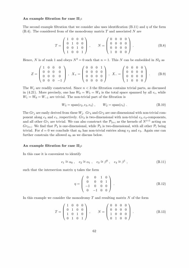
An example filtration for case II1:

The second example filtration that we consider also uses identification (B.11) and η of the form

(B.4). The considered from of the monodromy matrix T and associated N are

T =

1 0 0 00 1 0 00 0 1 01 0 0 1

, N =

0 0 0 00 0 0 00 0 0 01 0 0 0

. (B.8)

Hence, N is of rank 1 and obeys N2 = 0 such that n = 1. This N can be embedded in Sl2 as

Z =

1 0 0 00 0 0 00 0 0 00 0 0 −1

, X+ =

0 0 0 10 0 0 00 0 0 00 0 0 0

, X− =

0 0 0 00 0 0 00 0 0 01 0 0 0

. (B.9)

The Wj are readily constructed. Since n < 3 the filtration contains trivial parts, as discussed

in (4.21). More precisely, one has W6 = W5 = W4 is the total space spanned by all ei, while

W1 = W0 = W−1 are trivial. The non-trivial part of the filtration is

W3 = span(e2, e3, e4) , W2 = span(e4) . (B.10)

The Grj are easily derived from these Wj . Gr4 and Gr2 are one-dimensional with non-trivial com-

ponent along e4 and e1, respectively. Gr3 is two-dimensional with non-trivial e2, e3-components,

and all other Gri are trivial. We can also construct the P3+i as the kernels of N i+1 acting on

Gr3+i. We find that P4 is one-dimensional, while P3 is two-dimensional, with all other Pi being

trivial. For d = 0 we conclude that a0 has non-trivial entries along e2 and e3. Again one can

further constrain the allowed a0 as we discuss below.

An example filtration for case II2:

In this case it is convenient to identify

e1∼= α0 , e2

∼= α1 , e3∼= β0 , e4

∼= β1 , (B.11)

such that the intersection matrix η takes the form

η =

0 0 1 00 0 0 1−1 0 0 00 −1 0 0

. (B.12)

In this example we consider the monodromy T and resulting matrix N of the form

T =

1 0 0 00 1 0 01 0 1 00 1 0 1

, N =

0 0 0 00 0 0 01 0 0 00 1 0 0

. (B.13)

62

Hence, N is of rank 1 and obeys N2 = 0 such that n = 1. This N can be embedded in Sl2 as

Z =

1 0 0 00 0 0 00 0 0 00 0 0 −1

, X+ =

0 0 1 00 0 0 10 0 0 00 0 0 0

, X− =

0 0 0 00 0 0 01 0 0 00 1 0 0

. (B.14)

Again we easily construct the Wj , by first noting that n < 3 such that filtration contains

trivial parts (4.21). One has W6 = W5 = W4 is the total space spanned by all ei, while

W1 = W0 = W−1 are trivial. The non-trivial part of the filtration is

W3 = W2 = span(e3, e4) . (B.15)

The Grj are easily derived from these Wj . Gr4 and Gr2 are two-dimensional with non-trivial

component along e1, e2 and e3, e4, respectively. All other Gri are trivial. We can also construct

the P3+i as the kernels of N i+1 acting on Gr3+i. We find that P4 is one-dimensional, while P3

is two-dimensional, with all other Pi being trivial. For d = 0 we conclude that a0 has non-trivial

entries along e2 and e3. Again one can further constrain the allowed a0 as we discuss below.

Local classifications in the one-modulus case

While the presented examples seem only to represent specific choices of monodromy matrices,

they actually provide the key examples appearing in a classifications of allowed filtrations and

vectors a0. Considering 4× 4 representations it is possible to get quite far without assuming a

particular form for T but only using general constraints. In particular, since the Sl2 algebra is

invariant under unitary transformations one can use this freedom to eliminate components in

the most general matrices. Using this, and other constraints, an analysis of the one-modulus

case was performed in full generality in [66].

It was found that there are precisely three classes of N for one modulus, of which (B.5), (B.8)

and (B.13) are special examples. These are summarised in table B.1, where the first column

gives η and hence allows the match with the basis (αK , βK) define in (2.5).

Global classifications in the one-modulus case

Having summarised the classification of monodromy about a local point in the one-parameter

moduli space in table B.1, we now discuss some global aspects. In fact, it is possible to classify

also the global structure of the moduli space for such one-parameter Calabi-Yau threefolds that

have a moduli space P1/ 0, 1,∞. This was performed in [67] and here we summarize their

results. The moduli space P1/ 0, 1,∞ is parameterised by z and has three monodromy points.

The monodromy about z = 0 is maximally unipotent, so n = 3, and is therefore a large-complex

structure limit. The monodromy about z = 1 is of rank 1 and is the conifold locus.

The monodromy matrices about these loci satisfy the relation T0T1T∞ = 1. They can

therefore be specified by any two elements, which take the form

T0 =

1 0 0 01 1 0 00 m 1 00 0 1 1

, T1 =

1 −a −1 −10 1 0 00 0 1 00 0 0 1

. (B.16)

63

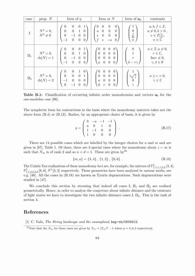
case prop. N form of η form or N form of a0 constants

IN4 = 0,N3 6= 0

0 0 0 10 0 1 00 −1 0 0−1 0 0 0

0 0 0 0a 0 0 0e b 0 0f e −a 0

10f2aπ

a, b, f ∈ Z,a 6= 0, b > 0 ,e ∈ Z[1

2 ],π ∈ C

II1N2 = 0,

rk(N) = 1

0 0 0 10 0 1 00 −1 0 0−1 0 0 0

0 0 0 00 0 0 00 0 0 0a 0 0 0

01τ

δ − τγ

a ∈ Z, a 6= 0,

τ ∈ C,Imτ 6= 0,γ, δ ∈ R

II2N2 = 0,

rk(N) = 2

0 0 1 00 0 0 1−1 0 0 00 −1 0 0

0 0 0 00 0 0 0a 0 0 00 c 0 0

1i√

ac

0γ

a ≥ c > 0,γ ∈ C

Table B.1: Classification of occurring infinite order monodromies and vectors a0 for theone-modulus case [66].

The symplectic form for contractions in the basis where the monodromy matrices takes not the

above form (B.4) or (B.12). Rather, by an appropriate choice of basis, it is given by

η =

0 −a −1 −1a 0 1 01 −1 0 01 0 0 0

. (B.17)

There are 14 possible cases which are labelled by the integer choices for a and m and are

given in [67], Table 1. Of these, there are 3 special cases where the monodromy about z =∞ is

such that N∞ is of rank 2 and so n = d = 1. These are given by35

m, a = 4, 4 , 1, 2 , 9, 6 . (B.18)

The Calabi-Yau realisations of these monodromy loci are, for example, the mirrors of P51,1,1,1,2,2 [4, 4],

P51,1,2,2,3,3 [6, 6], P5 [3, 3] respectively. These geometries have been analysed in various works, see

e.g. [48]. All the cases in (B.18) are known as Tyurin degenerations. Such degenerations were

studied in [47].

We conclude this section by stressing that indeed all cases I, II1 and II2 are realised

geometrically. Hence, in order to analyse the conjecture about infinite distance and the existence

of light states we have to investigate the two infinite distance cases I, II2. This is the task of

section 4.

References

[1] C. Vafa, The String landscape and the swampland, hep-th/0509212.

35Note that the N∞ for these cases are given by N∞ = (T∞)p − 1 where p = 4, 6, 3 respectively.

64

[2] N. Arkani-Hamed, L. Motl, A. Nicolis, and C. Vafa, The String landscape, black holes and

gravity as the weakest force, JHEP 06 (2007) 060, [hep-th/0601001].

[3] H. Ooguri and C. Vafa, On the Geometry of the String Landscape and the Swampland,

Nucl. Phys. B766 (2007) 21–33, [hep-th/0605264].

[4] D. Klaewer and E. Palti, Super-Planckian Spatial Field Variations and Quantum Gravity,

arXiv:1610.00010.

[5] E. Palti, The Weak Gravity Conjecture and Scalar Fields, JHEP 08 (2017) 034,

[arXiv:1705.04328].

[6] E. Palti, On Natural Inflation and Moduli Stabilisation in String Theory, JHEP 10 (2015)

188, [arXiv:1508.00009].

[7] F. Baume and E. Palti, Backreacted Axion Field Ranges in String Theory, JHEP 08 (2016)

043, [arXiv:1602.06517].

[8] I. Valenzuela, Backreaction Issues in Axion Monodromy and Minkowski 4-forms, JHEP 06

(2017) 098, [arXiv:1611.00394].

[9] S. Bielleman, L. E. Ibanez, F. G. Pedro, I. Valenzuela, and C. Wieck, Higgs-otic Inflation

and Moduli Stabilization, JHEP 02 (2017) 073, [arXiv:1611.07084].

[10] R. Blumenhagen, I. Valenzuela, and F. Wolf, The Swampland Conjecture and F-term

Axion Monodromy Inflation, JHEP 07 (2017) 145, [arXiv:1703.05776].

[11] A. Hebecker, P. Henkenjohann, and L. T. Witkowski, Flat Monodromies and a Moduli

Space Size Conjecture, JHEP 12 (2017) 033, [arXiv:1708.06761].

[12] M. Cicoli, D. Ciupke, C. Mayrhofer, and P. Shukla, A Geometrical Upper Bound on the

Inflaton Range, arXiv:1801.05434.

[13] R. Blumenhagen, D. Klaewer, L. Schlechter, and F. Wolf, The Refined Swampland Distance

Conjecture in Calabi-Yau Moduli Spaces, arXiv:1803.04989.

[14] W. Schmid, Variation of Hodge structure: the singularities of the period mapping, Invent.

Math. , 22:211–319, 1973.

[15] B. Heidenreich, M. Reece, and T. Rudelius, Emergence and the Swampland Conjectures,

arXiv:1802.08698.

[16] B. Heidenreich, M. Reece, and T. Rudelius, The Weak Gravity Conjecture and Emergence

from an Ultraviolet Cutoff, arXiv:1712.01868.

[17] L. Andrianopoli, M. Bertolini, A. Ceresole, R. D’Auria, S. Ferrara, P. Fre, and T. Magri,

N=2 supergravity and N=2 superYang-Mills theory on general scalar manifolds: Symplectic

covariance, gaugings and the momentum map, J. Geom. Phys. 23 (1997) 111–189,

[hep-th/9605032].

[18] B. Craps, F. Roose, W. Troost, and A. Van Proeyen, What is special Kahler geometry?,

Nucl. Phys. B503 (1997) 565–613, [hep-th/9703082].

65

[19] D. M. G. Kempf, F. F. Knudsen and B. Saint-Donat, Toroidal embeddings 1, Lect. Notes in

Math., vol. 339, Springer-Verlag, Berlin-New York (1973).

[20] A. Landman, On the picard-lefschetz transformation for algebraic manifolds acquiring

general singularities, Trans. Amer. Math. Soc. 181 (1973), 89-126.

[21] I. Garcıa-Etxebarria, T. W. Grimm, and I. Valenzuela, Special Points of Inflation in Flux

Compactifications, Nucl. Phys. B899 (2015) 414–443, [arXiv:1412.5537].

[22] C.-L. Wang, On the incompleteness of the Weil–Petersson metric along degenerations of

Calabi-Yau manifolds, Mathematical Research Letters 4, 157–171 (1997).

[23] C.-L. Wang, Aspects on Calabi–Yau moduli, (2016).

[24] T.-J. Lee, A Hodge theoretic criterion for finite Weil–Petersson degenerations over a

higher dimensional base, [arXiv:1604.06914 [math.AG]].

[25] E. Palti, Model building with intersecting D6-branes on smooth Calabi-Yau manifolds,

JHEP 04 (2009) 099, [arXiv:0902.3546].

[26] S. Cecotti, Supersymmetric Field Theories. Cambridge University Press, 2015.

[27] F. Denef, Supergravity flows and D-brane stability, JHEP 08 (2000) 050,

[hep-th/0005049].

[28] F. Denef, B. R. Greene, and M. Raugas, Split attractor flows and the spectrum of BPS

D-branes on the quintic, JHEP 05 (2001) 012, [hep-th/0101135].

[29] M. R. Douglas, B. Fiol, and C. Romelsberger, The Spectrum of BPS branes on a

noncompact Calabi-Yau, JHEP 09 (2005) 057, [hep-th/0003263].

[30] M. R. Douglas, D-branes, categories and N=1 supersymmetry, J. Math. Phys. 42 (2001)

2818–2843, [hep-th/0011017].

[31] P. S. Aspinwall, Some navigation rules for D-brane monodromy, J. Math. Phys. 42 (2001)

5534–5552, [hep-th/0102198].

[32] P. S. Aspinwall, R. L. Karp, and R. P. Horja, Massless D-branes on Calabi-Yau threefolds

and monodromy, Commun. Math. Phys. 259 (2005) 45–69, [hep-th/0209161].

[33] D. L. Jafferis and G. W. Moore, Wall crossing in local Calabi Yau manifolds,

arXiv:0810.4909.

[34] P. S. Aspinwall and M. R. Plesser, Decompactifications and Massless D-Branes in Hybrid

Models, JHEP 07 (2010) 078, [arXiv:0909.0252].

[35] E. Andriyash, F. Denef, D. L. Jafferis, and G. W. Moore, Bound state transformation

walls, JHEP 03 (2012) 007, [arXiv:1008.3555].

[36] P. Deligne, Theorie de Hodge: III, Publications Mathematiques de l’IHES 44 (1974) 5–77.

[37] M. Kerr, G. Pearlstein, and C. Robles, Polarized relations on horizontal SL(2)s, ArXiv

e-prints (May, 2017) [arXiv:1705.03117].

66

[38] C. Peters and J. Steenbrink, Mixed Hodge Structures. Ergebnisse der Mathematik und

ihrer Grenzgebiete. 3. Folge / A Series of Modern Surveys in Mathematics. Springer Berlin

Heidelberg, 2008.

[39] E. Cattani, A. Kaplan, and W. Schmid, Degeneration of Hodge Structures, Annals of

Mathematics 123 (1986), no. 3 457–535.

[40] E. Cattani and A. Kaplan, Polarized mixed hodge structures and the local monodromy of a

variation of hodge structure., Inventiones mathematicae 67 (1982) 101–116.

[41] J. Polchinski, Monopoles, duality, and string theory, Int. J. Mod. Phys. A19S1 (2004)

145–156, [hep-th/0304042]. [,145(2003)].

[42] B. Heidenreich, M. Reece, and T. Rudelius, Sharpening the Weak Gravity Conjecture with

Dimensional Reduction, JHEP 02 (2016) 140, [arXiv:1509.06374].

[43] M. Montero, G. Shiu, and P. Soler, The Weak Gravity Conjecture in three dimensions,

arXiv:1606.08438.

[44] B. Heidenreich, M. Reece, and T. Rudelius, Evidence for a Lattice Weak Gravity

Conjecture, arXiv:1606.08437.

[45] S. Andriolo, D. Junghans, T. Noumi, and G. Shiu, A Tower Weak Gravity Conjecture from

Infrared Consistency, arXiv:1802.04287.

[46] P. Candelas, X. De La Ossa, A. Font, S. H. Katz, and D. R. Morrison, Mirror symmetry

for two parameter models. 1., Nucl. Phys. B416 (1994) 481–538, [hep-th/9308083].

[AMS/IP Stud. Adv. Math.1,483(1996)].

[47] A. T. C. Doran, A. Harder, Mirror symmetry, Tyurin degenerations and fibrations on

Calabi-Yau manifolds, arXiv:1601.08110 [math.AG].

[48] J. Walcher, Calculations for Mirror Symmetry with D-branes, JHEP 09 (2009) 129,

[arXiv:0904.4905].

[49] A. N. Tyurin, Fano versus Calabi-Yau, The Fano Conference, Univ. Torino, Turin, 2004,

pp. 701–734.

[50] J. Calabrese and R. P. Thomas, Derived equivalent Calabi-Yau 3-folds from cubic 4-folds,

Math. Ann. 365 (2016), no. 1, 155–172.

[51] A. Strominger, Massless black holes and conifolds in string theory, Nucl. Phys. B451

(1995) 96–108, [hep-th/9504090].

[52] C. Vafa, A Stringy test of the fate of the conifold, Nucl. Phys. B447 (1995) 252–260,

[hep-th/9505023].

[53] N. Seiberg and E. Witten, Electric - magnetic duality, monopole condensation, and

confinement in N=2 supersymmetric Yang-Mills theory, Nucl. Phys. B426 (1994) 19–52,

[hep-th/9407087]. [Erratum: Nucl. Phys.B430,485(1994)].

[54] J. A. Harvey and A. Strominger, The heterotic string is a soliton, Nucl. Phys. B449 (1995)

535–552, [hep-th/9504047]. [Erratum: Nucl. Phys.B458,456(1996)].

67

[55] N. Arkani-Hamed, S. Dimopoulos, and S. Kachru, Predictive landscapes and new physics at

a TeV, hep-th/0501082.

[56] J. Distler and U. Varadarajan, Random polynomials and the friendly landscape,

hep-th/0507090.

[57] S. Dimopoulos, S. Kachru, J. McGreevy, and J. G. Wacker, N-flation, JCAP 0808 (2008)

003, [hep-th/0507205].

[58] G. Dvali and M. Redi, Black Hole Bound on the Number of Species and Quantum Gravity

at LHC, Phys. Rev. D77 (2008) 045027, [arXiv:0710.4344].

[59] G. Dvali, Black Holes and Large N Species Solution to the Hierarchy Problem, Fortsch.

Phys. 58 (2010) 528–536, [arXiv:0706.2050].

[60] D. Harlow, Wormholes, Emergent Gauge Fields, and the Weak Gravity Conjecture, JHEP

01 (2016) 122, [arXiv:1510.07911].

[61] D. Lust and E. Palti, Scalar Fields, Hierarchical UV/IR Mixing and The Weak Gravity

Conjecture, JHEP 02 (2018) 040, [arXiv:1709.01790].

[62] A. Ceresole, R. D’Auria, and S. Ferrara, The Symplectic structure of N=2 supergravity and

its central extension, Nucl. Phys. Proc. Suppl. 46 (1996) 67–74, [hep-th/9509160].

[63] M. Montero, Are tiny gauge couplings out of the Swampland?, JHEP 10 (2017) 208,

[arXiv:1708.02249].

[64] H. Ooguri and C. Vafa, Non-supersymmetric AdS and the Swampland, arXiv:1610.01533.

[65] A. Herraez, L. E. Ibanez, F. Marchesano, and G. Zoccarato, The Type IIA Flux Potential,

4-forms and Freed-Witten anomalies, arXiv:1802.05771.

[66] M. K. M. Green, P. Griffiths, Neron models and boundary components for degenerations of

hodge structure of mirror quintic type, Curves and Abelian Varieties (V. Alexeev, Ed.),

Contemp. Math 465 (2007), AMS, 71-145.

[67] C. F. Doran and J. W. Morgan, Mirror symmetry and integral variations of Hodge

structure underlying one parameter families of Calabi-Yau threefolds, in Calabi-Yau

varieties and mirror symmetry. Proceedings, Workshop, Mirror Symmetry 5, Banff,

Canada, December 6-11, 2003, pp. 517–537, 2005. math/0505272.

68